


1. Introduction
Verbal communication has been a defining feature of human civilization for millennia. Ramig & Verdolini (Reference Ramig and Verdolini1998) and Roy et al. (Reference Roy, Merrill, Gray and Smith2005) estimated from 3 % to 9 % of people in the United States alone suffer from some type of voice abnormality. These conditions can have powerful effects beyond a person's physical health, impacting the ability to work and interface with society, and ultimately affecting one's mental and emotional well-being. For this reason, the ability to understand, model and ultimately enable voice production remains critically important.
The work in this paper is focused on the connection between the momentum balance in time-varying glottal jets formed by flow through vibrating vocal folds, and the generation of sound. The research is built from a comprehensive, first-principles dynamics approach in which time-resolved measurements are used to compute every term in the streamwise integral momentum equation
This analysis is conducted in both phase-averaged and instantaneous forms using time-resolved DPIV and simultaneous measurement of pressure along the centreline of the vocal-fold model. The terms in (
1.1) are, in order of appearance, the time rate of change of streamwise momentum in the control volume, the flux of streamwise momentum across the open upstream and downstream control surfaces, the net streamwise pressure force (i.e. transglottal pressure force) acting on the inlet and outlet faces of the control volume, viscous drag along the vocal-fold sidewalls and net pressure drag on the vocal folds. Because flow and pressure are measured simultaneously over multiple oscillation cycles over a range of parameters, the full momentum balance provides a structured framework for assessing the various dynamical hypotheses that, until now, have been based heavily on kinematic observations. Using this approach, it is also possible to show how cycle-to-cycle variations in the glottal jet influence phase-averaged analysis. As such, this work both demonstrates a comprehensive, dynamics-based research paradigm for studying human phonation as well as presents new scientific findings.
1.1. Description of the flow and key parameters
A sequence of vocal-fold motions and associated flow across one oscillation cycle is shown schematically in figure 1. Each drawing represents a different time step in the cycle. Flow is from bottom to top. The glottis is the gap between the vocal folds through which air flows. By convention, the upstream side of the vocal folds is referred to as subglottal and downstream of the folds is supraglottal. Transglottal pressure, then, refers to the pressure difference between the higher subglottal and lower supraglottal pressures. In the remainder of this paper, the orientation is rotated 90° to the right relative to figure 1, so the supraglottal region and flow is to the right. The flow is defined to be in the positive x-direction.
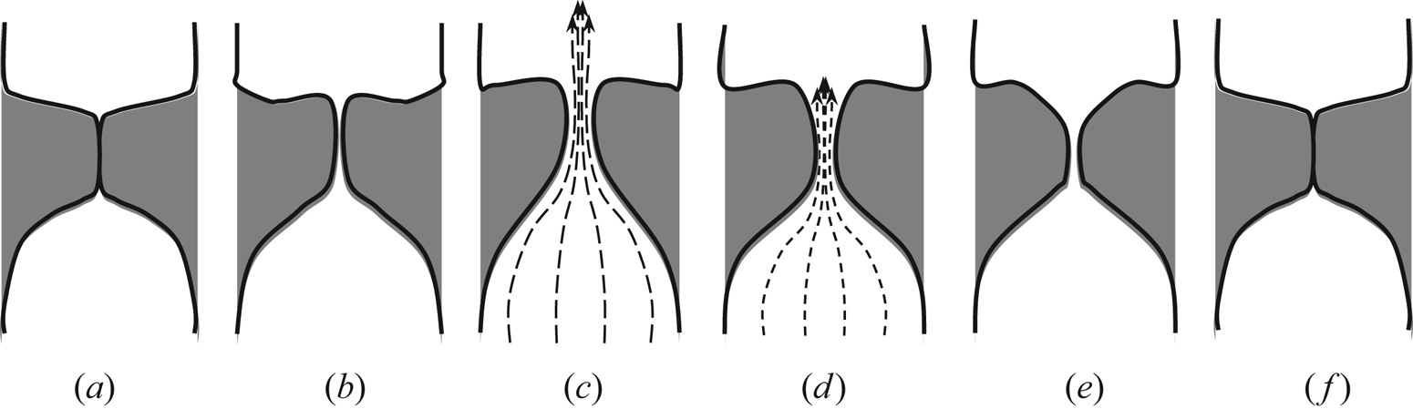
Figure 1. Schematic of vocal-fold motion showing opening (a–c) and closing (d–f) phases of one vocal-fold vibration cycle. Dashed arrows denote airflow through the glottis when it is open.
Figures 1(a) and 1(f) show the vocal folds at the beginning and end of the cycle, respectively. When the cycle begins, pressure from the lungs opens the glottis by pushing the folds upward, figure 1(b), and then outward, figure 1(c). Once opened, a jet, shown as dashed arrows, forms and the subglottal driving pressure decreases. As will be highlighted in § 1.3, the glottal jet has been observed to turn to one side or the other, sometimes switching directions across cycles and also exhibits three-dimensional behaviour as a function of geometry and frequency.
Later in the cycle, through combined aerodynamic pressure and elastic recoil effects, the vocal folds rock back and close, figures 1(d) and 1(e). The glottal jet pinches off and the folds return to their original position, figure 1(f). In human phonation the vocal folds do not always close completely, but when they do, they can remain closed for 80% to 120 % of the time that the glottis is open; the time between figures 1(b) and 1(e) approximately equals the time between figure 1(f) back to 1(a). The time the glottis is open is defined as To. In this work, the time open and the time closed are equal, so the total oscillation period is 2To.
There are three characteristic non-dimensional numbers for this flow: a Reynolds number and two dimensionless frequencies. The Reynolds number is based on maximum glottal opening, hmax, and the steady-state bulk jet velocity when the vocal folds are held fully open, Uss. The more commonly used non-dimensional frequency is the Strouhal number, defined as f hmax/Uss, where the vocal-fold oscillation frequency is f = 1/2To. In this paper, the reduced frequency introduced in Krane, Barry & Wei (Reference Krane, Barry and Wei2010), f* = f L/Uss, is used. The rationale is that the vocal-fold length, L, is a more appropriate length scale for the jet dynamics than the gap width.
There are two additional relevant frequencies referred to in this paper, fmodel and flife. The first, fmodel, is the model vocal-fold oscillation frequency, 1/2To. This corresponds to an equivalent life frequency, flife, that is 1500 times fmodel. This factor stems from multiplying the ratio of kinematic air and water viscosities,  ${\nu _{air}}/{\nu _{water}} = 15$, by the volume ratio of model to life scale (i.e. 103). Note that the velocity scale ratio, Ulife/Umodel, is then 150.
1.2. A brief review of vocal-fold models
Access to human vocal folds, due to the small size of the glottis and high vocal-fold vibration frequencies, continues to impede attempts to directly observe and quantify the phonation dynamics. For a comprehensive review of the literature on the fluid dynamics of human phonation, the reader is referred to Mittal, Erath & Plesniak (Reference Mittal, Erath and Plesniak2013). There have been a variety of vocal-fold models developed, ranging from in vivo and ex vivo, to those that include both driven and flow induced vibration.
Excised vocal folds, e.g. Jiang & Titze (Reference Jiang and Titze1993), Alipour, Jaiswal & Finnegan (Reference Alipour, Jaiswal and Finnegan2007), Khosla et al. (Reference Khosla, Muruguppan, Gutmark and Scherer2007), Oren, Khosla & Gutmark (Reference Oren, Khosla and Gutmark2014), Alipour, Finnegan & Scherer (Reference Alipour, Finnegan and Scherer2009) and Alipour, Finnegan & Jaiswal (Reference Alipour, Finnegan and Jaiswal2013), and in vivo models, e.g. Dollinger, Berry & Berke (Reference Dollinger, Berry and Berke2005), provide anatomically and physiologically correct representations of the highly complex geometry and biomechanical behaviour of real vocal folds. This realism is offset by challenges to reproducibility as each model geometry is unique and material properties of the excised folds and surrounding tissue change rapidly.
To address these issues, a variety of physical models that allow for more repeatable experiments have been used. Erath & Plesniak (Reference Erath and Plesniak2006a,Reference Erath and Plesniakb, Reference Erath and Plesniak2010) explored pulsatile two-dimensional flow through static asymmetric divergent models while Scherer, Shinwari & DeWitt (Reference Scherer, Shinwari and DeWitt2001) developed the so-called static M5 model to study symmetric and asymmetric glottis configurations. To overcome limitations of static models, Thomson, Mongeau & Frankel (Reference Thomson, Mongeau and Frankel2005) created complementary physical and numerical models using idealized size, shape and mechanical properties approximating those of human vocal folds. Subsequent studies (Pickup & Thomson Reference Pickup and Thomson2009; Murray & Thomson Reference Murray and Thomson2012) have produced physical vocal folds models with complex internal structure, incorporated three layers of different stiffness, consisting of cover, transition and body layers.
In order to focus on the source of phonatory flow variability, physical models with phase-coherent vocal-fold motion were developed. Coker et al. (Reference Coker, Krane, Reis and Kubli1996), and Mongeau et al. (Reference Mongeau, Francheck, Coker and Kubli1997) designed a life-sized mechanical model of human vocal folds driven by two actuating rods embedded in rubber. Barry, Krane & Wei (Reference Barry, Krane and Wei2004) developed a simplified scaled up, stepper motor driven model that executed a periodic motion across a model larynx. Peterson (Reference Peterson2007) used the same experimental setup investigated asymmetric model behaviour to explore conditions of paralysis and paresis. Sherman et al. (Reference Sherman, Lambert, Krane and Wei2019) built on this design to incorporate more modes of wall motion. Triep, Brücker & Schroder (Reference Triep, Brücker and Schroder2005) developed a driven model employing two counter-rotating elliptical cams to approximate the changing glottal profile during an oscillation cycle. Kucinschi et al. (Reference Kucinschi, Scherer, DeWitt and Ng2006) developed a driven mechanical model that executed two of the lower-order eigenmodes of the vocal folds studied computationally by Berry et al. (Reference Berry, Herzel, Titze and Krischer1994) and Titze & Martin (Reference Titze and Martin1989).
1.3. Glottal jet kinematics
There is an overlapping body of work addressing ‘traditional’ turbulence phenomena including coherent structures, asymmetries and three dimensionalities of the glottal jet. Scherer et al. (Reference Scherer, Shinwari and DeWitt2001) and Erath & Plesniak (Reference Erath and Plesniak2006a,Reference Erath and Plesniakb), for instance, addressed fundamental questions such as the occurrence of glottal jet asymmetry. Studies like these also raised interesting questions, such as the occurrence of asymmetric jet flows, phenomena observed even when the physical models are symmetric, and their dynamic relevance. Indeed, whether flows of these types actually occur in the human larynx motivated other researchers, including Triep et al. (Reference Triep, Brücker and Schroder2005) and Kucinschi et al. (Reference Kucinschi, Scherer, DeWitt and Ng2006), to examine more physiologically representative models.
Jet motions are, of course, important to speech sound production. This was discussed by Stevens (Reference Stevens1971), Shadle (Reference Shadle1985), McGowan (Reference McGowan1988), Hirschberg (Reference Hirschberg1992), Krane (Reference Krane2005), Howe & McGowan (Reference Howe and McGowan2005, Reference Howe and McGowan2007, Reference Howe and McGowan2011) and McGowan & Howe (Reference McGowan and Howe2007), based on the foundational aeroacoustic theory laid by Lighthill (Reference Lighthill1952). A key point discussed in Lighthill (Reference Lighthill1952), Curle (Reference Curle1955) and Crighton (Reference Crighton1975) is that sound generated by an acoustically compact (incompressible) flow is an integrated effect of the accelerations across the source volume. In this context, glottal flow variability, relative to the vocal-fold motion, is associated with the dynamics and energy fluctuations that couple to the acoustics through the equations of motion.
Indeed, there is a growing body of experiments in which qualitative features of the glottal jet, e.g. coherent structures, three dimensionalities, jet deflection and switching, are examined in the context of sound production. Examples include Neubauer et al. (Reference Neubauer, Zhang, Miraghaie and Berry2007), Drechsel & Thomson (Reference Drechsel and Thomson2008) and more recently, Sidlof et al. (Reference Sidlof, Doaré, Cadot and Chaigne2011), Krebs et al. (Reference Krebs, Silva, Sciamarella and Artana2012), Lodermeyer et al. (Reference Lodermeyer, Tautz, Becker, Döllinger, Birk and Kniesburges2018) and Farbos de Luzan et al. (Reference Farbos de Luzan, Khosla, Oren, Maddox and Gutmark2018, Reference Farbos de Luzan, Oren, Maddox, Gutmark and Khosla2020). In general, these works focus principally on coherent structures and do not quantify the forces, i.e. dynamics, behind those kinematic features.
It is important to note that there are a number of computational studies that focused on sound generated during phonation, including Zheng et al. (Reference Zheng, Mittal, Xue and Bielamowicz2011), Kaltenbacher et al. (Reference Kaltenbacher, Zörner, Hüppe and Sidlof2014), Mattheus & Brücker (Reference Mattheus and Brücker2018) and Sadeghi et al. (Reference Sadeghi, Kneisburges, Falk, Kaltenbacher, Schützenberger and Döllinger2019). Perhaps because a body of experimental work does not (yet) exist to examine the relationship between jet dynamics and sound, these computational studies have a heavy focus on kinematics like their experimental counterparts. A notable exception is found in Kaltenbacher et al. (Reference Kaltenbacher, Zörner, Hüppe and Sidlof2014) where three-dimensional maps of acoustic source terms are plotted. They demonstrate that these maps are highly complex and can only be extracted from full three-dimensional data sets including velocity and pressure. In general, however, these studies did not address the global dynamics of glottal jets, or how the aerodynamic forces imparted by it relate to sound production.
1.4. Glottal jet dynamics
To be useful in terms of clinical measures for voice pathology and treatment, spatial and temporal information from the more kinematics-based approaches highlighted above need to be reframed in terms of the fluid forces that tie to acoustic source strength. Accordingly, the detailed flow information needs to be understood concurrently from an integral momentum perspective. This is discussed in Zhang, Mongeau & Frankel (Reference Zhang, Mongeau and Frankel2002a,Reference Zhang, Mongeau and Frankelb), Krane (Reference Krane2005), Howe & McGowan (Reference Howe and McGowan2007) and McPhail, Campo & Krane (Reference McPhail, Campo and Krane2019). A key point is that vocal-fold drag is a direct measure of voice aeroacoustic source strength, which is an integral quantity.
The body of work focused on dynamics is far smaller than that focused on kinematics. Deverge et al. (Reference Deverge, Pelorson, Vilain, Lagrée, Chentoug, Willems and Hirschberg2003) directly measured pressure using two symmetric vocal folds where one was fixed and the other moved. The flow exhausted directly to atmosphere. They recorded time-resolved traces of sub-, supra- and transglottal pressure for three different geometries. Since there were no flow measurements, however, they could not examine the full dynamics of the problem. Mattheus & Brücker (Reference Mattheus and Brücker2018) also presented a measured transglottal pressure trace, but it was used only to validate their computations.
Beyond providing kinematic information, DPIV has been used to compute complex terms in the turbulent transport equations, cf. Hsu et al. (Reference Hsu, Grega, Leighton and Wei2000) and Grega, Hsu & Wei (Reference Grega, Hsu and Wei2002). In addition, methods for extracting the pressure field from DPIV data have been developed by Dabiri et al. (Reference Dabiri, Bose, Gemmel, Colin and Costello2014) and Lambert et al. (Reference Lambert, Pipinos, Baxter, Chatzizisis, Ryu, Leighton and Wei2018). These state-of-the-art approaches have not yet been applied to glottal flows. A simplified inviscid momentum equation approach was used by Oren et al. (Reference Oren, Khosla and Gutmark2014) to estimate the pressure associated with vortices generated during the closing of excised canine laryngeal vibration. This study was neither time resolved, nor was the full force balance examined.
The open opportunity therefore exists to couple dynamics with kinematics by concurrently conducting control-volume analyses on the same data used to extract detailed full flow-field information. This has been shown to be an invaluable tool for understanding complex fluid-structure interaction (FSI) dynamics. Examples include vortex-induced vibration (VIV) of flexibly mounted cylinders, e.g. Benaroya & Wei (Reference Benaroya and Wei2000) and Voorhees et al. (Reference Voorhees, Dong, Atsavapranee, Benaroya and Wei2008), and strong frequency dependence on cycle-to-cycle variations in oscillating duct flows, Sherman et al. (Reference Sherman, Lambert, Krane and Wei2019). In the VIV work of Voorhees et al. (Reference Voorhees, Dong, Atsavapranee, Benaroya and Wei2008), a slight mismatch between the vortex shedding frequency and the cylinder's natural frequency was shown to modulate the strength and coherence of the Kármán vortices from cycle to cycle. This was further shown to create a modulated forcing function that led to a beating behaviour of the cylinder. This was incorporated into the reduced-order analytical model developed in Benaroya & Wei (Reference Benaroya and Wei2000).
Cycle-to-cycle variations were also observed in the oscillating constriction experiments of Sherman et al. (Reference Sherman, Lambert, Krane and Wei2019). For a nominally symmetric and highly repeatable mechanism, the unsteady jet could vary significantly in both strength and direction from one cycle to the next, phenomena which were found to be highly frequency dependent. Very similar behaviours were observed in the present experiments even though the geometries and facilities were quite different.
These FSI examples serve to motivate the present work. Time-resolved measurements of the full flow field provide critical insights into the underlying unsteady turbulent glottal jet kinematics and dynamics. It is the integral control-volume analysis that, in turn, links the fluid dynamics to the acoustics. The experimental features that enable this integral analysis are: (i) simultaneous time-resolved velocity field and pressure measurements along the vocal-fold model and (ii) the resulting ability to directly compute all of the terms in the integral momentum equation.
1.5. Problem statement
Mittal et al. (Reference Mittal, Erath and Plesniak2013) broadly divided flow studies of glottal jets into works focusing on coherent structures, asymmetries, and three-dimensionalities; categorizations that still largely apply today. Much of this work has focused on kinematic analysis of a single oscillation cycle or phase averaging of multiple cycles with or without acoustic measurements or computations.
To place the current work in context and to demonstrate its impact on the field of phonation, it is worthwhile to clearly identify what is known, what is not known and issues at the boundaries which are either accepted but not fully established, or established but not widely adopted. In terms of experimental fluid mechanics methodologies applied to the study of phonation: (i) DPIV has become widely used in vocal-fold experiments, (ii) phase locking and phase averaging are common techniques for examining glottal jet flows, (iii) highly resolved time traces of sub-, supra- and transglottal pressure have been made and (iv) acoustics measurements have been coupled to kinematic flow observations.
In terms of kinematic observations, three things are universally accepted: (i) even for highly symmetric geometries and vocal-fold motions, the glottal jet has a high propensity to turn away from the glottal centreline, (ii) this jet direction can change from one cycle to the next resulting in often unpredictable jet switching and (iii) depending on the vocal-fold geometry, jet three-dimensionalities, i.e. variations in the z-direction, are commonly observed. Finally, two things about the relationship between flow and acoustics are known. First, cycle-to-cycle variations in flow correlate to cycle-to-cycle variations in sound. And second, sound generation is related to volume flow.
What is not known or understood about phonation is the dynamics; only the temporal evolution of transglottal pressure as a function of vocal-fold motion has been well described. Critical open questions that can only be addressed through examination of the fluid dynamics include: (i) What causes the observed kinematic cycle-to-cycle variations, e.g. jet switching? (ii) Which, if any, cycle-to-cycle variations in flow are actually important to sound production, and if so, how? And (iii) what causes deviations from quasi-steady flow when vocal folds open and just before they close, and whether this is relevant in terms of sound production.
In addition, there are three issues warranting further examination. The first is that acoustic source strength is directly proportional to vocal-fold drag. This was discussed in Hirschberg (Reference Hirschberg1992) and Zhang et al. (Reference Zhang, Mongeau and Frankel2002a,Reference Zhang, Mongeau and Frankelb) and relates back to the foundational theory of Curle (Reference Curle1955), Crighton (Reference Crighton1975) and Howe (Reference Howe1975). While McPhail et al. (Reference McPhail, Campo and Krane2019) argued that the driving transglottal pressure force is nearly equal to (or at least a surrogate for) vocal-fold drag, these types of dynamics-based studies have yet to be widely incorporated into research in the field.
The remaining two issues deal with a consensus that glottal flows are quasi-steady without definitive proof in the literature. Specifically, first, while it is widely accepted that the glottal jet is quasi-steady in a phase-averaged sense, this has only been established in the middle of the oscillation cycle and not when the vocal folds have just opened or when they are about to close. Second, research into quasi-steadiness is largely limited to low (adult male) frequencies.
In summary, to deepen the understanding of phonation, it is essential to understand the interrelationship between acoustics, kinematics and dynamics, i.e. to deploy the streamwise integral momentum equation, (1.1) to the understanding of glottal jet dynamics with the goal of providing insight and understanding into the role of the jet motions on sound production. Temporally resolved DPIV velocity-field measurements are simultaneously coupled with time-resolved pressure measurements through a 10× scaled up vocal-fold model. This builds on the work of Barry et al. (Reference Barry, Krane and Wei2004) and Krane, Barry & Wei (Reference Krane, Barry and Wei2007), Krane et al. (Reference Krane, Barry and Wei2010) which presented only velocity-field measurements. These new measurements allow both a phase-averaged examination of the integral momentum equations as well as the consideration of cycle-to-cycle variations. Thus, it is now possible to directly address the three questions raised above. The phase-averaged analysis makes it possible to identify the principal contributions to the vocal-fold drag, i.e. the principal aeroacoustic source strength. At the same time, examination of individual cycles yields insights into phonation and potentially ways in which the flow may influence sound quality and perception.
It should be acknowledged here that actual acoustics measurements are not possible in an incompressible flow facility. By linking the kinematics of jet phenomena, however, in both the phase-averaged and cycle-to-cycle senses, with the dynamics, and, in turn knowing the relationship between the momentum and acoustics equations, a framework is created to fully understand the role of the glottal jet variations on sound production.
Cases reported in this paper correspond to nominally normal phonation cases, in which the vocal folds move symmetrically and close fully. Both frequency and Reynolds number effects are examined. This work provides a baseline for ongoing studies into conditions where the vocal folds do not fully close and vocal-fold motions are asymmetric. Specific questions addressed in this study are:
• whether the driving transglottal pressure force from the lungs does indeed serve as a surrogate for vocal-fold drag;
• whether the momentum flux and unsteady inertia terms contribute to voiced sound production and quality;
• how the flow dynamics varies with Reynolds number and frequency;
• how terms in the streamwise momentum equation are affected by cycle-to-cycle variations; and
• what causes cycle-to-cycle variations.
2. Apparatus
Experiments were conducted using a 10× scaled up vocal-fold model in a large free-surface water tunnel. The vocal-fold models were the same as those used in Barry et al. (Reference Barry, Krane and Wei2004) and Krane et al. (Reference Krane, Barry and Wei2007, Reference Krane, Barry and Wei2010). The important difference in the current apparatus was the addition of time-resolved pressure measurements along the axis of the glottal duct. These were made through video recording of manometers. Flow measurements were obtained using DPIV. A top-view schematic of the experimental apparatus is shown in figure 2.
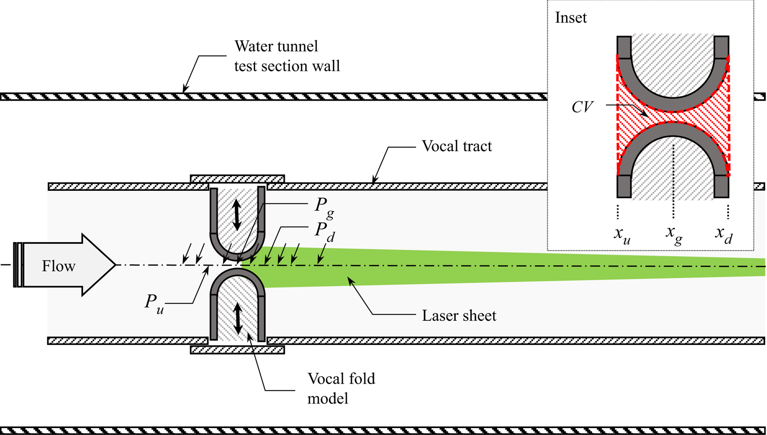
Figure 2. Top-view installation drawing of scaled-up vocal-fold model including stepper motor (not shown) driven vocal folds and vocal tract installed in a free-surface water tunnel. Flow is left to right. A horizontal laser sheet is directed upstream with camera (not shown) looking up from underneath the tunnel. Locations of ten pressure taps are indicated with arrows; the upstream, Pu, glottal, Pg, and downstream, Pd, taps are indicated. The inset drawing shows the control volume in red and the upstream, glottal and downstream locations, xu, xg and xd, respectively.
The glottal model consisted of a 28 cm × 28 cm × 366 cm (inside measure) duct with a square, closed cross-section, into which two vocal-fold models were inserted. The entire assembly was constructed using 1.27 cm thick acrylic. The vocal-fold models consisted of 12.7 cm diameter half-cylinders fixed to the ends of rectangular boxes such that the assembly was 14 cm wide × 12.7 cm in streamwise length × 28 cm high. As shown in figure 2, each model fit into an opening on either side of the glottal duct, 45.7 cm downstream of the duct entrance. The geometry downstream of the vocal-fold models was the remaining 306.7 cm of the square duct.
A 1.27 cm thick back plate with two 2.54 cm circular stainless-steel guideposts was used to constrain the motion of each vocal fold in the cross-stream direction. Linear Teflon bearings were used to minimize friction and eliminate vibration as the vocal folds moved in and out on the posts. The gaps between the model and the openings in the duct wall were less than 0.01 cm. Further, there were openings at the tops and bottoms of the back plates so that as the vocal folds moved, fluid behind the vocal folds would be exchanged with the fluid outside of the glottal duct; there was no measurable leakage between the vocal folds and the duct walls.
Each vocal-fold model was driven by a Servo System® stepper motor using a worm gear and linear stage. Both motors were controlled from a single timing signal to ensure symmetry of motion. The pitch of the lead screw was 0.0635 cm meaning that approximately 17.5 motor revolutions, or 3500 individual motor steps, were required for the vocal-fold models to go from fully closed to fully open and vice versa. For the lowest- and highest-frequency cases, the stepper motor rotation speeds were 2.4 and 4.5 rev s−1, respectively.
The new feature added to this model was a set of ten pressure taps drilled along the centreline of the duct ceiling. Each tap was 0.16 cm in diameter. Defining the upstream and downstream faces of the vocal-fold models as xu and xd, respectively, and the location of the glottis, i.e. the point of contact of the two opposing models, as xg, the streamwise locations of the pressure taps were  $(x-{x_u})/({x_d}-{x_u}) =-0.5$, −0.25, 0, 0.25, 0.5, 0.75, 1.0, 1.25, 1.5 and 2.0. Each tap was connected to an approximately 200 cm length of 0.64 cm inner diameter flexible tubing. All tubes were the same length and were each in turn connected to a glass tube with 0.32 cm inner diameter. The tubes were affixed to form a manometer bank which was mounted vertically outside the water tunnel test section. A discussion of frequency response of this system is provided in § 3.4.
The full glottal duct assembly was mounted in a free-surface water tunnel built by Rolling Hills Research. It had a custom-designed test section measuring 61 cm in width, 91.4 cm in depth and 500 cm in length. Flow was driven by a single frequency-controlled axial flow pump that is vibration isolated from the tunnel with flexible rubber couplings. The maximum flow rate of the pump was approximately 10 000 lpm.
The assembly was placed on a set of legs, 15.24 cm high, so that the tunnel sidewalls and floor were equidistant from the glottal duct. The closed top of the duct was submerged to approximately 5 cm below the free surface. This was deep enough to minimize any wave effects at the inlet of the duct, but not so deep that the stepper motors that moved the model vocal fold and wiring would come in contact with the water.
DPIV measurements were made using a Phantom Miro 310 high-speed video camera and a Quantel Evergreen EVG00200 dual pulse Nd:YAG laser. The laser had a maximum power of 200 mJ per pulse with a repetition rate of 15 Hz. Flow was seeded with 10 μm silver-coated glass spheres from Potter Industries. The camera, vocal-fold stepper motors and laser were synchronized by a Berkeley Nucleonics 565 Pulse Delay Generator.
Simultaneous video recordings of the time-varying manometer levels were made using a Raspberry Pi camera. The Raspberry Pi camera framed at 30 f.p.s. driven by its own onboard clock. The entire system, including vocal folds, laser, DPIV camera and Raspberry Pi camera, however, were all triggered by a common pulse from the pulse delay generator.
The two-dimensional (i.e. unit depth) integral control volume is shown in figure 2 as an inset and appears as the red shaded region. The upstream and downstream faces are co-located with the upstream and downstream faces of the vocal-fold models and defined to extend across the entire width of the duct. Contributions to velocity integrals, such as the momentum flux term in (1.1), are identically zero everywhere along the flat parts of the vocal folds where there is no flow. The ‘lateral faces’ of the control volume are defined to be the vocal-fold walls. As such, the area (or volume) within the control volume changes with time. This variable geometry becomes important in the unsteady inertia term, the calculation of which is described in § 4.4 and Appendix A.
3. Methods
3.1. Flow conditions
Building on the work of Barry et al. (Reference Barry, Krane and Wei2004), Krane et al. (Reference Krane, Barry and Wei2007, Reference Krane, Barry and Wei2010) and Sherman et al. (Reference Sherman, Lambert, Krane and Wei2019), the goal of the present research was to provide a fuller understanding the momentum balance in glottal jets with an eye toward direct coupling to sound production. This study focused on symmetric vocal-fold motions over a range of Reynolds numbers and reduced frequencies characteristic of the adult human male voice.
Two data sets were compiled, one at a fixed frequency with four different Reynolds numbers, and the other at a fixed Reynolds number with four different frequencies. One case was common to both sets such that a total of seven separate cases were examined. Recalling from § 1.1 that the time from open to close was defined as To and the total oscillation period was 2To, the vocal-fold model frequencies, fmodel = 1/2To, were 0.035 Hz, 0.045 Hz, 0.055 Hz and 0.065 Hz. Adjusting for the 10× scale of the vocal-fold models relative to physiological scale, and the fact that the kinematic viscosity of air is 15 times that of water, these frequencies correspond to life-scale frequencies, flife, of 52.5 Hz, 67.5 Hz, 82.5 Hz and 97.5 Hz, respectively. The Reynolds numbers (based on hmax ≈ 22 mm) examined were 3560, 5350, 7200 and 8100 corresponding to steady-state jet speeds, Uss, of 16.2, 23.8, 31.6 and 36.0 cm s−1, respectively. The four Reynolds numbers were studied at the highest model frequency, 0.065 Hz (flife = 97.5 Hz) and the four frequencies were studied at Re = 7200.
For every case studied, tunnel speed was set, with the vocal folds closed, and allowed to run for a minimum of thirty minutes before the vocal-fold motions were initiated. This ensured that the bulk flow around the outside of the duct model was steady. Two empirical observations verified that the flow around and downstream of the duct model was steady and laminar. First, the tunnel free surface is extremely sensitive to vortices. Even the smallest, weakest vortices that attach to the free surface create dimples that are clearly visible because of the optical distortions they create. No such disturbances were observed either along the outer edges of the duct or in the wake. Second, the free-surface mirror used to reflect the DPIV laser sheet upstream into the measurement region was mounted to a cantilever. Any unsteadiness in the flow hitting the mirror would cause vibrations which would, in turn, vibrate the laser sheet. To ensure the mirror did not affect flow inside the duct, it was placed roughly a metre downstream of the duct exit. With the duct length downstream of the vocal folds being over three metres, the total distance from the laser sheet to the vocal folds was more than four metres. This is a tremendous optical lever, yet there was absolutely no vibration of the laser sheet.
In terms of the effects of vocal-fold opening on the bulk flow and in the subglottal region of the duct, Krane et al. (Reference Krane, Barry and Wei2007) argued that the change in total blockage area of the duct model caused by vocal-fold motions was very small and would therefore have little effect on the subglottal pressure. That is, there would not be a marked decrease in pressure at the duct entrance that would, in turn, create vortices and other disturbances of the flow entering the glottal region. This was verified in this experiment. With the vocal folds closed the total blockage area of the duct was 28.9 % of the cross-sectional area of water in the test section. When the vocal folds were fully opened, the blockage area of the duct decreased by less than 1 % to 28.1 %. As will be seen in § 4.3, specifically figures 7 and 8, the effect of vocal-fold opening on subglottal pressure could be observed but had negligible impact on the flow.
To ensure adequate sample sizes for phase-averaging, a minimum of twenty oscillation periods were captured for each of the seven cases. To fully assess cycle-to-cycle variability, it would have been desirable to run the oscillations continuously and capture one complete data set for each case; this would have ensured that start-up transients could be eliminated or minimized. Camera storage limitations, however, prevented this. Thus, for the four cases at 0.065 Hz, three sets of eight consecutive oscillations were captured. For the 0.035 Hz, 0.045 Hz and 0.055 Hz cases, five sets of four, six sets of four and three sets of seven consecutive oscillations were captured, respectively.
In addition, pressure and velocity measurements were also made for the four Reynolds numbers under steady-state conditions where the vocal folds were fixed in the full-open position. One thousand vector fields were captured for these steady-state full-open cases over a span of 67 s. Pressure measurements were made when the vocal folds were in the fully closed position and the water tunnel pump was running at settings corresponding to the four Reynolds numbers. Since there was no flow through the vocal-fold models, flow measurements were unnecessary for these cases.
3.2. Vocal-fold motions
One goal of this research has been to simplify the model geometry and motions enough to identify the essential dynamics present in actual phonation. As noted earlier, the vocal-fold motions were the same as those used in Barry et al. (Reference Barry, Krane and Wei2004) and Krane et al. (Reference Krane, Barry and Wei2007, Reference Krane, Barry and Wei2010). The vocal folds opened at a nominally constant speed to a maximum opening, hmax, closed at the same constant speed and then remained closed for a time equal to the sum of the opening and closing times.
Sample traces of the vocal-fold motions were presented in Krane et al. (Reference Krane, Barry and Wei2007); in addition, a sequence of individual oscillation cycles is presented later in § 5.3 (figure 16). In the previous and current studies, there were small deviations from the target motion when the folds first started opening, when they changed direction and when they closed, i.e. at t/2To = 0, 0.25 and 0.5, respectively. Specifically, time traces of the actual vocal-fold motions were slightly rounded around these three time points. This was simply because the stepper motors were incapable of instantaneous accelerations. The non-dimensional time intervals, during which the actual vocal-fold motions differed from the start, reverse and end of the idealized triangular trajectory, were approximately 0.05 in duration.
The position of the vocal folds was determined by the number of steps the motors turned and was verified directly from the DPIV video images. An edge-detection algorithm was used to locate the two vocal folds in each video frame and to track the glottal opening. For all cases studied, the average maximum glottal opening, hmax, was 2.2 cm with an overall standard deviation of 0.11 cm. For every individual run (of four to eight consecutive oscillations), however, the maximum deviation in hmax was less than 0.05 cm. The greatest variation in glottal opening was from run-to-run and not from cycle-to-cycle. And, as will be shown, the greatest cycle-to-cycle variation in transglottal pressure and jet dynamics actually occurred for cases where the vocal-fold motions were most repeatable. Therefore, while there were variations in vocal-fold motions as great as ±2.5 %, these were not the primary cause of cycle-to-cycle variations in the associated flows.
For the Re = 8100 case, however, the static friction on one of the vocal folds was higher than the other. This resulted in a delayed start by approximately 0.04To, leading to a slightly higher speed than the desired profile as the vocal fold overcame the starting friction, followed by a slightly lower speed. It will be shown that the effects of this perturbation were minimal. The most interesting effects were actually observed for the Re = 7200 cases where the vocal-fold speeds were constant for the majority of their motion.
3.3. DPIV measurements
Time-resolved flow-field measurements were made at the mid-height of the glottal model. The camera field of view was 21.9 cm × 16.4 cm in the x and y-directions, respectively. For all measurements in this study, the pixel resolution was 54.8 pixels cm−1. The flow was illuminated with a dual pulse Nd:YAG laser which, using a cylindrical lens, formed an approximately 0.1 cm thick light sheet, which was about 14 cm wide at the vocal-fold models. The laser sheet entered through the sidewall of the water tunnel test section, far downstream of the glottal duct, and was reflected upstream along the duct centreline at the duct mid-height using a 10 cm × 12.7 cm front-surface mirror. The laser sheet is illustrated schematically in figure 2.
DPIV image pairs were captured with the digital video camera below the water tunnel test section, oriented upward toward the vocal-fold models. As will be shown in § 4, the camera was positioned so that the flow was left to right and the glottis was just inside the left edge of the field of view. The capture rate for image pairs was 15 Hz for a minimum of 230 vector fields per oscillation cycle (at the highest frequency). For the two lower speeds studied, the time between images in a pair, δt, was set to 3 ms, and for the two faster speeds, δt was 1.5 ms.
The stepper motors, DPIV camera and laser were all driven and synchronized using a master clock on the pulse delay generator. The pulse generator had multiple output channels. One pulse was generated at the start of every vocal-fold oscillation cycle which was used to start and synchronize the pressure measurement system. Other channels fired the two laser heads and the camera image capture. A single computer key stroke set the entire system in motion.
DPIV vector fields were computed using a two-stage cross-correlation algorithm described in Hsu (Reference Hsu2000) and Hsu et al. (Reference Hsu, Grega, Leighton and Wei2000). The program first used 128 × 128 pixel windows to obtain coarse displacement fields. In the second, or fine, correlation stage, smaller windows were used. In this study these windows were 32 × 32 pixels. The correlation windows in the second image of each image pair were offset relative to its counterpart in the first image by an integer pixel amount determined from the coarse correlation stage. Four-times oversampling was used so that, in this case, vectors were 8 pixels apart in both directions, corresponding to 0.146 cm in physical space.
In a detailed analysis of the current DPIV algorithm, Hsu et al. (Reference Hsu, Grega, Leighton and Wei2000) showed the measurement uncertainty for an individual velocity measurement was less than 0.03 pixels. Willert & Gharib (Reference Willert and Gharib1991) provided a more conservative estimate of 0.1 pixels. For a maximum pixel displacement of approximately five pixels along the jet centreline, the uncertainty of the velocity measurements is between 0.6 % and 2 %. The uncertainty for maximum jet velocity, volume flow rate and the unsteady inertia term in the streamwise integral momentum equation, presented in § 4, would then be between 0.6 and 2 % of their respective maximum values. Since momentum flux and dynamic pressure are proportional to streamwise velocity squared, the uncertainty of those measurements is between 1.2 % and 4 % of their respective maxima. Of course, assuming the error is stochastic, phase averaging and integration should reduce these uncertainties.
3.4. Pressure measurements
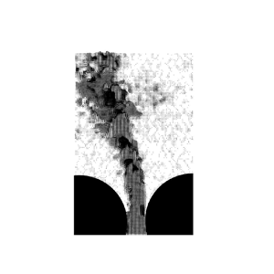
As noted previously, the new and unique experimental feature of this study was the inclusion of time-resolved pressure measurements along the axis of the model glottal duct. The locations of the ten pressure taps were described in § 2. Water heights in the glass manometer bank were imaged and recorded using a Raspberry Pi camera at 30 f.p.s. and a resolution of 80 pixels cm−1. Sample video images of the pressure distribution along the glottal duct are shown in figure 3. Figures 3(a) and 3(b) show the pressure distribution when the vocal folds are closed and opening, respectively. The ability to measure changes in manometer column height is evident in these images.

Figure 3. Sample movie frames showing streamwise pressure distributions along the glottal duct (a) when the vocal folds are closed, and (b) when they are opening. Manometers corresponding to the upstream, Pu, glottal, Pg, and downstream, Pd, taps are indicated. To indicate measurement resolution, a dashed line was drawn along the menisci of the water columns in (a) and replicated in (b). The solid line in (b) was drawn along the menisci of the water columns in (b).
Prior to every experimental run, a few drops of a dilute soap solution were injected into the top of each manometer. This flattened and reduced surface tension of the meniscus, allowing the water column to accurately track pressure changes in the flow.
For each oscillation cycle in each run, the Raspberry Pi camera was triggered by a pulse from the master clock on the Berkeley Nucleonics pulse delay generator. It was observed that there was a very slight mismatch in the clock rates of the master clock on the pulse delay generator and the Raspberry Pi; over the duration of the longest experimental run, 123 s, the net time differential between the master clock and the Raspberry Pi clock could be several milliseconds. For each cycle, therefore, the master clock triggered the Raspberry Pi which then captured images using its on-board clock until the pulse delay generator signalled the start of another oscillation period. In this manner, the DPIV and Raspberry Pi video capture rates for flow and pressure measurement, respectively, were synchronized to within ±1 ms over each vocal-fold oscillation period.
At the start and end of each day, a set of images of the manometer columns was captured with zero flow through the water tunnel. This ensured that the manometer heights were all level in the absence of a pressure gradient and provided the reference zero gauge pressure for each manometer. As noted in § 2, a small amount of soap solution was injected into each manometer at the beginning of the day to eliminate surface tension effects, the dominant source of error and damping.
For the small displacements in this study, the manometers could conservatively be assumed to be critically damped with a natural frequency of,  ${\omega _n} = \sqrt {g/L} $, of 2.2 rad s−1 (where g is the gravitational acceleration = 9.81 m s−1 the tube length, L = 2 m). For a step change in pressure, then, it would take ~1 s for a manometer to record 90 % of that change. This was most relevant when the vocal folds first opened, changed directions and closed. Since these are not step changes, the primary effect on pressure measurements would be up to a ~0.5 s time lag after changes in vocal-fold motion; this corresponds to t/2To ≈ 0.03 for the highest-frequency case. There would not, however, be a significant loss in accuracy, particularly for the phase-averaged measurement. For the highest-frequency case, for instance, the vocal-fold speeds are 0.29 cm s−1 and they move in each direction for 3.85 s. Except for the passage of individual jet vortices, the manometer response was fast enough to capture the first-order pressure variations.
In order to quantify pressures in each manometer, the video images were converted to binary using a threshold level that clearly and sharply defined the menisci of each water column. Since the images of each meniscus would be several pixels thick vertically, the centroid of each meniscus along the manometer centreline was computed. This centroid location was used as the column height for that manometer in that video image. Using a series of regularly spaced markers, visible on the left of the sample images in figure 3, these locations were converted to pressures in Pascals.
Analysis of the pressure measurement apparatus and methodology revealed that the most significant source of uncertainty was the determination of the meniscus location. Close examination of figure 3 shows that the meniscus is about 0.05 cm thick, or 5 Pa. For these experiments, the maximum transglottal pressure difference was approximately 85 Pa. While the algorithm to find the centroid of the meniscus has sub-pixel resolution, a conservative pressure measurement resolution estimate of ±5 Pa is less than 6 % of the maximum pressure differential of this investigation.
4. Results
Simultaneous DPIV and pressure measurements were made in a scaled up vocal-fold model in a large free-surface water tunnel. Seven separate cases were examined, across four different frequencies and four different Reynolds numbers. The model frequencies, fmodel, were 0.035 Hz, 0.045 Hz, 0.055 Hz and 0.065 Hz corresponding to life frequencies, flife, of 52.5 Hz, 67.5 Hz, 82.5 Hz and 97.5 Hz, respectively. The Reynolds numbers were 3560, 5350, 7200 and 8100. These Reynolds numbers were studied at the highest frequency, equivalent to 97.5 Hz, while the four frequencies were studied at Re = 7200. Results from these experiments are presented in this section. For reference, measurements of pressure and velocity were also made for the steady-state cases where the vocal folds were fixed in their full-open position and subsequently in the fully closed position at the four different Reynolds numbers; these are the ‘steady-state’ cases.
4.1. Velocity and pressure across a phase-averaged oscillation cycle
The interrelation between spatially and temporally resolved flow and pressure measurements across the glottal model is highlighted in this sub-section. Figure 4 is a sequence of six panels showing phase-averaged DPIV vector fields with associated streamwise pressure distributions at non-dimensional times from t/2To = −0.05 to 0.45. This spans the time just before the vocal folds begin to open to just before they close. For comparison, instantaneous DPIV vector fields are presented later in § 5.3 (figure 15). Flow is left-to-right with the vocal folds masked in white. The vector fields show every other vector and have been scaled and aligned with the x-axis of the pressure plots. Observe that a small patch of spurious vectors has been masked in the lower right corners of figure 4(c–f). These are artifacts from a single oscillation cycle and lie outside of where any analysis was done.

Figure 4. Sequence of six streamwise pressure distributions and corresponding phase-averaged DPIV vector fields along the glottal model at t/2To = (a) −0.05, (b) 0.05, (c) 0.15, (d) 0.25, (e) 0.35 and (f) 0.45 for Re = 7200, flife = 97.5 Hz (f* = 0.0261). Note that (x − xu)/(xd − xu) = 0, 0.5 and 1.0 are the upstream face, glottis and downstream face, respectively.
Pressure is shown in the form of a pressure coefficient,  $(P(x)-{P_{d{-}closed}})/ ({P_{u{-}closed}}-{P_{d{-}closed}})$, where Pu-closed and Pd-closed are the steady-state pressures at the upstream and downstream faces of the model when the folds are closed. Non-dimensionalized positions, $(x-{x_u})/({x_d}-{x_u}) = 0$, 0.5 and 1.0, correspond to the upstream face, xu, glottis, xg, and downstream face, xd, respectively. As noted in § 3.4, a conservative estimate of pressure uncertainty was ±5 Pa or ±0.07 using the pressure coefficient defined above.
Before considering individual panels, observe that the non-dimensional subglottal pressure values in figure 4 vary by less than ±0.1 over the entire phase-averaged oscillation cycle. There is a small decrease when the vocal folds open and a recovery when they close. This is similar to what is observed in the human airway.
Turning now to the individual time steps, Figure 4(a) corresponds to t/2To = −0.05, shortly before the vocal folds begin to open. There is no mean flow and the pressure coefficient upstream of the glottis is unity. Downstream of the glottis, the pressure is also constant, although at a dimensionless value of approximately −0.15. This indicates that even though the vocal folds remain closed for a time equal to To between openings, there is insufficient time for the pressure to fully equilibrate to the steady-state closed levels such that the downstream pressure coefficient returns to zero. To put this in perspective, except for the highest frequencies at the highest Reynolds numbers, the time required for the glottal jet to traverse the 3 m duct length downstream of the vocal folds is longer than the time the vocal folds are closed; and this assumes the jet continues to move at its maximum velocity.
In figure 4(b), the vocal folds have begun to move and are at 20 % of the maximum opening. This corresponds to t/2To = 0.05. The phase-averaged starting jet is visible in the DPIV vector field and can be seen curving to the right (downward in the figure) away from the centreline. This is evidence of the Coanda effect, which has been discussed in multiple studies including Triep & Brücker (Reference Triep and Brücker2010), Mattheus & Brücker (Reference Mattheus and Brücker2011, Reference Mattheus and Brücker2018) and Sherman et al. (Reference Sherman, Lambert, Krane and Wei2019).
The direction the jet takes may be different for successive oscillations. In subsequent time steps, the phase-averaged jet appears broad, and in some instances, bifurcated. This is evidence of cycle-to-cycle variations similar to those presented in Sherman et al. (Reference Sherman, Lambert, Krane and Wei2019) and will be discussed in § 5.3. Observe that at this early stage, the streamwise pressure distribution has not yet significantly changed.
By t/2To = 0.15, shown in figure 4(c), the focal folds are at 60 % of their full separation, hmax. It can be seen that the pressure in the upstream half of the vocal-fold model, (x − xu)/(xd − xu) = 0.25, decreases while pressure downstream of the glottis increases. Upstream of the model, the non-dimensional pressure also decreases slightly, by approximately 0.07. This reflects the fact that the opening of the vocal folds releases upstream pressure which is then carried downstream. The DPIV vector field shows that by this time, the jet has traversed across the entire streamwise field of view. Notice that the phase-averaged jet appears to have bifurcated with a stronger jet downward (i.e. to the right). This indicates the range of variability of the jet direction over the twenty-four oscillation cycles comprising the ensemble. The asymmetry of the phase-averaged jet indicates that on average the flow turned either to the left or the right.
At t/2To = 0.25, given in figure 4(d), the vocal folds have reached their fully open position, hmax. The pressure at (x − xu)/(xd − xu) = 0.25 is approximately 20 % less than its value when the folds were closed, cf. figure 4(a). At the same time, the supraglottal pressures are approximately 20 % greater than Pd-closed.
The vocal folds close over the time interval 0.25 ≤ t/2To ≤ 0.5. Figure 4(e) corresponds to the time t/2To = 0.35 when the vocal folds are again at 60 % of hmax but are now closing. As they close, flow accelerates through the glottis. This is due to the combined effects of flow inertia and the additional flux, i.e. squeezing, by the closing folds. The pressure at (x − xu)/(xd − xu) = 0.25 reaches its lowest value because of the acceleration, while the supraglottal pressures begin to decrease. At the same time, the subglottal pressure increases by a small amount so that the pressure drop in the upstream half of the model reaches its local maximum.
Figure 4(f) shows the flow and pressure just before the vocal folds close. They are now 80 % closed, i.e. h = 0.2hmax, at t/2To = 0.45. The phase-averaged velocity field indicates that the jet has pinched off despite the fact that the folds are not yet fully closed, although this may be due to the thinness of the jet relative to the DPIV interrogation region. One can also see a small over-pressure upstream of the model and a significant under pressure in the supraglottal region. This decrease in supraglottal pressure continues after the vocal folds close, as was indicated in figure 4(a). As will be discussed in § 5.3, the residual motions and incomplete pressure recovery may contribute to perceptually relevant cycle-to-cycle variations.
4.2. Phase-averaged time traces of kinematic flow quantities
This sub-section contains time traces of basic kinematic flow quantities commonly used in the literature, e.g. Mongeau et al. (Reference Mongeau, Francheck, Coker and Kubli1997), Triep & Brücker (Reference Triep and Brücker2010), Mattheus & Brücker (Reference Mattheus and Brücker2018) and Krane et al. (Reference Krane, Barry and Wei2007, Reference Krane, Barry and Wei2010), among others. They are included here for completeness and are important for subsequent examination of flow dynamics presented in § 4.4.
Figure 5 shows phase-averaged time traces of maximum jet velocity, uj, along the vocal-fold exit plane, xd, for the four frequencies at Re = 7200 in figure 5(a) and the four Reynolds numbers at flife = 97.5 Hz in figure 5(b). Similar plots appear in Mongeau et al. (Reference Mongeau, Francheck, Coker and Kubli1997) and Krane et al. (Reference Krane, Barry and Wei2007). In these plots, uj has been non-dimensionalized by the averaged glottal jet bulk velocity, Uss, measured under fully open, steady-state conditions at the corresponding Reynolds numbers. For this and all subsequent traces, time is non-dimensionalized by the oscillation period, 2To, where t/2To = 0 and 0.5 correspond to when the vocal folds begin to open and when they close. In addition, vertical dashed lines have been placed at t/2To = 0.25 and 0.5 to indicate when the vocal folds are fully open and fully closed, respectively.

Figure 5. Time traces of maximum jet velocity across the vocal-fold exit plane for (a) the four oscillation frequencies at Re = 7200, and (b) the four different flow speeds at the highest frequency corresponding to a life frequency of 97.5 Hz. Dotted vertical lines indicate the times, t/2To = 0.25 and 0.5, when the vocal folds are fully opened and when they return to fully closed.
For quasi-steady flow, maximum jet velocity traces should nominally follow a top-hat profile with a time delay equal to L/2uj, the time required for the jet to traverse from the glottis to the exit plane. Once the vocal folds close, the maximum velocity will diminish to zero after an equivalent delay.
One can observe, however, humps around t/2To = 0.35 in every trace in figure 5. These are due to acceleration in the jet as the vocal folds begin to close. The height of the humps above the initial plateau are more pronounced with increasing frequency. Side peaks around t/2To = 0.05 and 0.45 are caused by the starting and pinch-off vortices that form as the vocal folds open and shut, respectively. Smaller spikes spaced along the traces, most noticeable at the lowest frequency in figure 5(a), are likely caused by individual vortices in the glottal jet passing the exit plane.
Deviations from the top-hat profile are also apparent for the different Reynolds numbers in figure 5(b). The lowest Reynolds number case appears most similar to a top hat. However, the maximum dimensionless jet velocity, uj/Uss, is significantly smaller than for the higher Reynolds numbers. Based on review of subsequent results, it is believed that this is primarily a frequency effect. Recall that reduced frequency, f*, is inversely proportional to velocity; the lowest Reynolds number case also happens to be the highest reduced frequency. With that in mind, if the lowest Reynolds number curve (which is the highest reduced frequency) in figure 5(b) were plotted on figure 5(a), that curve would continue the observed frequency dependence trend.
Phase-averaged traces of volume flow rate (per unit depth) across the vocal-fold exit plane are given in figure 6. The volume flow rate was computed by integrating the phase-averaged streamwise velocity across the vocal-fold exit plane at each time step. Following the convention of Krane et al. (Reference Krane, Barry and Wei2007, Reference Krane, Barry and Wei2010) and Triep & Brücker (Reference Triep and Brücker2010), data were non-dimensionalized by steady-state bulk velocity, Uss, and maximum glottal opening, hmax. Time was scaled by 2To.

Figure 6. Time traces of volume flow rate across the vocal-fold exit plate for (a) the four oscillation frequencies at Re = 7200, and (b) the four different flow speeds at flife = 97.5 Hz. Dotted vertical lines indicate the times, t/2To = 0.25 and 0.5, when the vocal folds are fully opened and when they return to fully closed.
Dependence on frequency at Re = 7200 is shown in figure 6(a). The lowest-frequency trace is an isosceles triangle centred at t/2To = 0.25 corresponding to when the vocal folds are fully opened. In addition, the maximum non-dimensional flow rate is slightly greater than 0.9. These two observations are consistent with the quasi-steady flow assumption.
With increasing frequency, however, the traces increasingly tilt to the right and the peak value of Q(t)/Uss hmax decreases. The smaller flow rates indicate that the glottis has started closing before the jet reaches steady-state conditions. The tilt is a manifestation of the jet being pinched off by the closing vocal folds. Both the tilting and reduced non-dimensional flow rate are visible for the two lowest Reynolds number cases in figure 6(b). Recalling that these two cases are also the highest f* cases studied, this again appears to be a frequency effect versus a Reynolds number effect.
It is worth noting the presence of weak flow reversals after the vocal folds close. Since the measurement plane is located at the vocal-fold exit plane, xd, the measured reversal is caused by residual recirculation after the jet pinches off. It is conjectured that residual motions explain why the supraglottal pressure does not fully recover, see figure 4(a). As will be discussed in § 5.3, these residual motions are also likely responsible for jet switching.
4.3. Phase-averaged pressure traces
Time traces of phase-averaged pressure coefficients are shown for the four different frequencies at Re = 7200 in figure 7, and the four Reynolds numbers at flife = 97.5 Hz in figure 8. In both figures, the phase-averaged pressure at the upstream face of the vocal-fold model, Pu, figures 7(a) and 8(a), at the glottis, Pg, figures 7(b) and 8(b), and at the exit plane, Pd, figures 7(c) and 8(c), are referenced to the mean downstream exit pressure when the vocal folds are closed, Pdo, and normalized by the mean transglottal pressure difference when the folds are closed, Puo − Pdo. For these and subsequent pressure plots, Puo and Pdo were the time-averaged values of the phase-averaged pressure signals at the upstream face, Pu, and downstream face, Pd, over the time interval, 0.85 ≤ t/2To ≤ 0.95. This interval was chosen to best represent the supraglottal and subglottal pressures when the vocal folds were closed; recall from figure 4 that the supraglottal pressure does not reach the steady-state closed value, Pd-closed. Time is again non-dimensionalized by the full oscillation period, 2To. While direct comparison is not possible, data shown here qualitatively agree with those reported in Deverge et al. (Reference Deverge, Pelorson, Vilain, Lagrée, Chentoug, Willems and Hirschberg2003) and Mattheus & Brücker (Reference Mattheus and Brücker2018).

Figure 7. Time traces of (a) upstream, (b) glottal and (c) downstream pressure coefficients for the four oscillation frequencies at Re = 7200. Dotted vertical lines indicate the times, t/2To = 0.25 and 0.5, when the vocal folds are fully opened and when they return to fully closed.

Figure 8. Time traces of (a) upstream, (b) glottal and (c) downstream pressure coefficients for the four different Reynolds numbers at flife = 97.5 Hz. Dotted vertical lines indicate the times, t/2To = 0.25 and 0.5, when the vocal folds are fully opened and when they return to fully closed.
It can be seen in figure 7(a) that as the vocal folds open the upstream pressure decreases by approximately 10 %. When the folds reach their maximum open position and begin to close, t/2To ≈ 0.25, the subglottal pressure begins to increase and overshoots by approximately 10 % when the folds close. The decrease is due to the release of pressure as the folds open while the increase is a result of restricting flow on the upstream, or subglottal, side when the folds start to close. Shortly after closure, Pu quickly settles back to Puo, although for the highest frequency, the return to Puo takes a comparatively longer non-dimensional time.
The glottal and supraglottal pressures, figures 7(b) and 7(c), increase as the vocal folds open and subglottal pressure is released. As the folds close, downstream pressure decreases due to the jet acceleration. After closure, the glottal and supraglottal pressures return toward, but never reach, the steady-state downstream pressure. The maximum variations in pressure are approximately 70 % of the pressure drop for the closed vocal folds, Puo − Pdo. Similar patterns can be seen in figure 8.
The interesting features in figures 7 and 8 are the distinct trends in frequency and Reynolds number. In figure 7(c), non-dimensional subglottal pressure levels increase with increasing frequency. For the highest-frequency case corresponding to flife = 97.5 Hz, the maximum dimensionless pressure is approximately five times that at flife = 52.5 Hz. The maximum pressure occurs later in the cycle, for successively higher frequencies. This is consistent with the increased acceleration of the jet as the vocal folds close and causes a relatively large pressure, (Pd − Pdo)/(Puo − Pdo) = 0.25, at the highest frequency.
The glottal pressures, figure 7(b), show similar frequency dependences as the supraglottal pressures, figure 7(c). The distinct difference is for the highest-frequency case, flife = 97.5 Hz. During opening, the maximum pressure is actually lower than the next two lower frequencies. It is not clear why this is the case. It is conjectured that the flow separation point may move relative to the three lower frequencies. This is a region where the pressure measurement could be very sensitive to the pressure tap location. Recall that the shape of the maximum jet velocity trace for the highest-frequency was decidedly different than for the lower three frequencies as seen in figure 5(a); the jet acceleration was delayed at the highest frequency. This is a question for further study.
There are consistent Reynolds number trends for both glottal and supraglottal pressures in figure 8. At face value, peak-to-peak pressure differences were greatest for the lowest Reynolds number which would seem counter-intuitive. Recalling, however, that the lowest Reynolds number is also the highest reduced frequency, the trends align with those observed in figure 7. As such, frequency effects may be more important than Reynolds number effects at least with respect to pressure and within the parameter range of this study. This is explored in § 4.4 below.
Finally, the waviness of the pressure traces particularly in figure 8(a) for the upstream pressure trace in the lowest Reynolds number case is worth noting. This is believed to be a manifestation of cycle-to-cycle variations which are most prevalent at the highest frequency. This will be discussed in greater detail in § 5.3.
4.4. Phase-averaged dynamics; terms in the streamwise integral momentum equation
The five terms comprising the integral streamwise momentum equation
 \begin{equation}{C_{inertia}} + {C_m} = {C_p} + {C_{f\;shear}} + {C_{D(vf)}},\end{equation}
are presented in this section. This is written in dimensionless form where terms in (1.1) are non-dimensionalized by (Puo − Pdo)Sduct. Starting with the right-hand side, the driving pressure force is the transglottal pressure multiplied by the cross-sectional area of the glottal duct. Non-dimensionalization identically results in the transglottal pressure coefficient shown in figures 9(a) and 9(b) for constant frequency and Reynolds number, respectively. Since the subglottal pressure, Pu, does not vary greatly across the oscillation cycle, phase-averaged traces of transglottal pressure coefficient look similar to the downstream pressure traces in figures 7(c) and 8(c). Data in figure 9 are in agreement with similar measurements by Deverge et al. (Reference Deverge, Pelorson, Vilain, Lagrée, Chentoug, Willems and Hirschberg2003) and computations by Mihaescu et al. (Reference Mihaescu, Khosla, Murugappan and Gutmark2010). As discussed previously, the peak-to-peak amplitude increases and the maximum pressure occurs later with increasing f*. This includes the lowest Reynolds number case, figure 9(b), which is also the highest f*.

Figure 9. Phase-averaged transglottal pressure time traces for (a) the four oscillation frequencies at Re = 7200, and (b) the four different flow speeds at flife = 97.5 Hz. The corresponding non-dimensional supraglottal pressure differences for the same cases are shown in (c) and (d), respectively. Dotted vertical lines indicate the times, t/2To = 0.25 and 0.5, when the vocal folds are fully opened and when they return to fully closed.
It is interesting to observe that the maxima in the transglottal pressure peak occur before the vocal folds close. If one were to assume that the pressure increase, nominally between when the vocal folds start to close, t/2To = 0.25, and when they fully close, t/2To = 0.5, is due to the inertial of the flow pushing past the glottis and the increasing blockage of the closing folds, then the peak should occur roughly when the folds close and not before. As can be seen in figure 9(a), the maximum transglottal pressure occurs as early as t/2To ≈ 0.4. As such, the effect of increasing blockage is not sufficient to fully understand the dynamics of glottal closure.
The phase-averaged supraglottal pressure difference, that is, the pressure difference between the glottis and downstream exit plane, (Pg − Pd), for constant flow speed and constant oscillation frequency, are shown in figures 9(c) and 9(d), respectively. It is interesting to observe that in figure 9(d), this supraglottal pressure difference is essentially zero when the vocal folds are open for the two lowest and the highest tunnel speeds at the highest oscillation frequency. In figure 9(c), however, the supraglottal pressure difference appears to be slightly positive for the three lowest oscillation frequencies. For Re = 7200 and the highest frequency, the pressure difference is slightly negative when the folds are open. For all cases there is a positive peak when the folds close and a small positive pressure.
One must be very careful in drawing conclusions about figures 9(c) and 9(d) because of the sensitivity to location and size of the pressure tap at the glottis. There is a single contact point (vertical line to be precise) at which the vocal folds make contact. But the pressure tap at the glottis is 0.16 cm in diameter. Therefore, it is likely that there was some degree of spatial averaging both upstream and downstream of that point of contact. Further, measurements of Pg will be highly sensitive to the jet separation point. With these things in mind, the key feature of these plots that can be extracted is that (Pg − Pd) is small in comparison with the transglottal pressure. The pressure gradient along the jet, then, appears to play a negligible dynamic role in phonatory airflow.
Time traces of vocal-fold drag for the four frequencies at Re = 7200 and for the four Reynolds numbers at flife = 97.5 Hz. are shown in figures 10(a) and 10(b), respectively. Vocal-fold drag was estimated using the pressure measurements at the upstream and downstream faces of the vocal-fold models as well as the two stations located one quarter and three quarters along the streamwise vocal-fold model length, i.e. (x − xu)/(xd − xu) = 0.25 and 0.75. The drag was computed as the difference of the upstream and downstream pressures multiplied by the area of the flat part of the model protruding into the duct, plus the difference of the pressures at (x − xu)/(xd − xu) = 0.25 and 0.75 multiplied by the projected area of the curved portion of the models, i.e. the radius of the cylindrical section times the duct height. The force coefficients were defined using the transglottal pressure when the vocal folds were closed, Puo − Pdo, and the glottal duct cross-sectional area.

Figure 10. Time traces of vocal-fold drag for: (a) the four oscillation frequencies at Re = 7200, and (b) the four different flow speeds at flife = 97.5 Hz. Dotted vertical lines indicate the times, t/2To = 0.25 and 0.5, when the vocal folds are fully opened and when they return to fully closed.
It can be seen that the driving pressure force, figure 9 and vocal-fold drag, figure 10 are both qualitatively and quantitatively similar. The peak-to-peak differences in the drag force are smaller than for the transglottal pressure force, and the drag force traces do not necessarily start and end at unity. In addition, the shape of the drag force traces in the range, 0 ≤ t/2To ≤ 0.4, are rounder than for the driving pressure force. This is most noticeable in comparing figures 9(b) and 10(b).
Similarities between figures 9 and 10 are not surprising. The primary differences between the drag and driving pressure force are the pressure distribution around the cylindrical parts of the vocal-fold models and the fact that the projected frontal area of the folds decrease and increase as the folds open and close, respectively. The salient point is that the transglottal pressure force does indeed serve as a surrogate for vocal-fold drag, as discussed by McPhail et al. (Reference McPhail, Campo and Krane2019).
The third term on the right-hand side of the streamwise momentum equation is the viscous drag term. Work by Sherman et al. (Reference Sherman, Lambert, Krane and Wei2019) demonstrated that this is negligibly small for these flows. This can also be seen using scaling arguments. Starting with the formula for wall shear stress in a two-dimensional planar Poiseuille flow, one can write a shear force coefficient consistent with the non-dimensionalization used in figures 9 and 10
 \begin{equation}{C_{{\,f_{shear}}}} = \; \frac{{\frac{h}{2}\frac{{\partial P}}{{\partial x}}\; {S_{wall}}}}{{({P_{uo}} - \; {P_{do}}){S_{duct}}}}.\end{equation}
Setting h to hmax and conservatively setting ∂P/∂x = (Puo − Pdo)/L, as the largest pressure gradient in the glottis and Swall to be the entire length of the vocal-fold model, L (i.e. area per unit depth), then the maximum value of  ${C_{{\,f_{shear}}}}$ reduces to ${h_{max}}/2W$ where W is the width of the duct. For this model, the maximum possible shear force coefficient would be 0.04. This is an over-prediction because the maximum shear force does not act over the entire model length and the transglottal pressure is at least 20 % less than Puo − Pdo when the flow is at its fastest. As such, a more realistic estimate of the maximum shear coefficient would be 0.01. This value is consistent with turbulent channel flow measurements of Schultz & Flack (Reference Schultz and Flack2013) for a channel width of 2.2 cm and a bulk velocity of 36 cm/sec, the highest jet speed in this study. This all supports the assertion that shear forces in this flow are negligible.
Turning next to the left-hand side of (1.1), or (4.1) in dimensionless form, traces of momentum flux coefficient for the four frequencies at Re = 7200 are shown in figure 11(a) while traces for the four Reynolds numbers at the highest frequency appear in figure 11(b). In the plots, momentum flux, non-dimensionalized by (Puo − Pdo)Sduct, is plotted as a function of t/2To. Momentum flux values were calculated integrating the local streamwise velocity squared across the width of the model exit plane.

Figure 11. Traces of integral streamwise momentum flux across the vocal-fold exit plane for: (a) the four frequencies at Re = 7200, and (b) the four flow speeds at flife = 97.5 Hz. Note the net momentum flux into the control volume is an order of magnitude smaller than the outward flux. Dotted vertical lines indicate the times, t/2To = 0.25 and 0.5, when the vocal folds are fully opened and when they return to fully closed.
Note that the momentum flux across the vocal-fold inlet plane of the was not included because velocity measurements were not made in the upstream half of the model. A simple order of magnitude estimate from continuity, however, shows that the momentum flux into the control volume is ~10 % of the outflow momentum flux. Define the streamwise velocity at the vocal-fold model inlet to be Uu and recall that for this model the width of the duct width is approximately ten times the maximum glottal width, hmax. From continuity, neglecting effects of the vocal-fold wall motions, the glottal velocity is 10Uu. Because of viscosity, the flow separates from the vocal-fold walls immediately downstream of the glottis and forms a coherent jet. Assume, to first order, that the jet width at the exit plane remains h, and the velocity remains 10Uu within the jet and zero everywhere on the exit plane outside of the jet. The momentum flux across the vocal-fold exit plane will then be  $100U_u^2h$ while it will be $U_u^2(10h)$ across the inlet plane. Thus, the momentum flux entering the vocal-fold model is an order of magnitude smaller than the flux leaving the model.
The key point of figure 11 is that, although small, momentum flux is not negligible. Over the range, 0.1 ≤ t/2To ≤ 0.4, the maximum value of the momentum flux coefficient is around 0.24. This occurs nominally when the vocal folds are fully open. Examination of figure 11(a) reveals that for the lowest-frequency case, the momentum flux trace is symmetric about t/2To ≈ 0.24. For increasing frequencies, the maximum values decrease and the traces lean to the right. That these trends in f* continue in figure 11(b) is consistent with the volume flow traces shown in figure 6.
The final term to be examined is the unsteady inertia term, Cinertia, or ![]() in dimensional form. Time traces of this term are shown in figure 12. As with previous plots, the four frequencies at Re = 7200 appear in figure 12(a) while the four Reynolds number cases at f = 0.065 Hz are in figure 12(b). A description of how the quantity was computed is provided in Appendix A. The non-dimensionalization was the same as that used for other terms in the momentum equation.
in dimensional form. Time traces of this term are shown in figure 12. As with previous plots, the four frequencies at Re = 7200 appear in figure 12(a) while the four Reynolds number cases at f = 0.065 Hz are in figure 12(b). A description of how the quantity was computed is provided in Appendix A. The non-dimensionalization was the same as that used for other terms in the momentum equation.

Figure 12. Time traces of the unsteady inertia term in the streamwise integral momentum equation for: (a) the four oscillation frequencies at Re = 7200, and (b) the four different flow speeds at the highest frequency corresponding to a life frequency of 97.5 Hz. Dotted vertical lines indicate the times, t/2To = 0.25 and 0.5, when the vocal folds are fully opened and when they return to fully closed.
The main feature of figure 12 is that the unsteady inertia term is in general even smaller than the momentum flux term. Observe also that the unsteady term is largest in magnitude when the folds first open and when they close. The acceleration is positive when the vocal folds are opening and the glottal jet is forming. Conversely, it is negative when the vocal folds are closing and the jet is getting pinched off. In figure 12(b), it can be seen that the largest magnitudes of the non-dimensional inertia term occur at the lowest Reynolds number, i.e. the highest reduced frequency, f*. In this regard, it is not surprising that the unsteady acceleration would be most pronounced for the lowest Reynolds number.
5. Discussion
5.1. Frequency and Reynolds number dependence
At the outset, it is worth commenting on the frequency range covered in this study. The actual range of frequencies examined was just under a factor of two, 52.5 Hz ≤ flife ≤ 97.5 Hz. Since the maximum frequency, flife = 97.5 Hz lies within the fundamental frequency range of adult males, this study has physiological relevance in its own right. Note, however, that the lowest Reynolds number case corresponds to f* = 0.0511, which is almost twice the f* = 0.0261 value of the highest-frequency case at Re = 7200. As such, this study provides insights into frequencies beyond the nominal range examined.
Frequency dependencies of phase-averaged kinematic and dynamic quantities have been highlighted throughout the preceding section. It was shown in § 4.2 that as frequency increases, flow accelerates through the glottis after the vocal folds start to close. This acceleration appears as an increasingly pronounced hump in the maximum jet velocity around t/2To = 0.3 in figure 5, and a leaning of the volumetric flow time traces to the right with increasing f* in figure 6. In the phase-averaged pressure traces in § 4.3, figures 7 and 8, supraglottal pressure minima decrease in magnitude with increasing frequency and the location of the peaks shifts toward t/2To = 0.5, i.e. when the vocal folds close.
In terms of the dynamics, it was shown in figures 9 and 10 in § 4.4 that the transglottal pressure force and the vocal-fold drag increases in magnitude with increasing frequency. The maximum streamwise momentum flux, presented in figure 11, decreased and occurred later in the cycle with increasing frequency; this was correlated with maxima in volume flow rate. Finally, inertia effects became more pronounced with increasing f*, specifically when the vocal folds first started opening and when they shut. However, even at the highest f*, the magnitude of the inertia forces was an order of magnitude smaller than the vocal-fold drag.
Discerning Reynolds number effects in this study is less straightforward because varying flow speed affects both Re and f* even when the oscillation frequency is held constant. From a phase-averaged perspective, frequency effects appear to dominate Reynolds number effects. For example, for a fixed f*, one would expect that transglottal pressure would increase with increasing Reynolds number because transglottal pressure increases with flow speed. However, figure 9(b) shows the opposite; the effects of increasing flow speed are much more consistent with f* trends observed in figure 9(a) than they are with what one would expect to see if Reynolds number were truly an independent variable. Still, Reynolds number effects become more evident when looking at cycle-to-cycle variations and will be examined in greater detail in § 5.3.
5.2. The dynamics of glottal jets
A key contribution of this paper to the human phonation literature is the ability to examine the entire momentum balance across the complete oscillation cycle. In this section, focus is on the phase-averaged balance. Cycle-to-cycle variations are addressed in the following sub-section.
To begin, it is important to revisit the foundational premise of this paper. As discussed in § 1, the goal of this study is to identify the flow features that contribute most to phonatory sound production. Because vocal-fold drag has been identified as the source of sound, these features may be ranked in terms of how they contribute to vocal-fold drag. For this, the reader is referred back to the control volume shown in figure 2 containing the fluid moving between the vocal folds.
For this analysis, the first term in (1.1) is reformulated using mass conservation, to break out the bulk unsteady acceleration and acceleration due to wall motion, and the pressure force integral into driving pressure force and vocal-fold drag, yielding
Here, Vxj is the glottal volume between axial location x and xd, the axial location of the control-volume outflow face. The orders of magnitude of these terms are
 \begin{gather}{\rho _0}\frac{\textrm{d}}{{\textrm{d}t}}\int_{{x_u}}^{{x_d}} {{u_j}{S_j}\,\textrm{d}x} \sim {\rho _0}\frac{{{u_j}{h_{max}}{L_G}}}{{{T_a}}}L,\end{gather}
 \begin{gather}{\rho _0}\frac{\textrm{d}}{{\textrm{d}t}}\int_{{x_u}}^{{x_d}} {{{\dot{V}}_{xd}}\,\textrm{d}x} \sim {\rho _0}{L^2}{L_G}\frac{{{h_{max}}}}{{T_o^2}},\end{gather}
 \begin{gather}({P_u} - P)S\sim \Delta PS\sim {\rho _0}u_j^2S,\end{gather}
where Ta is a time scale describing the duration of the sharp rise at the beginning of the cycle, and the rapid fall of jet velocity, uj, at the control-volume exit, as seen in figure 5. In addition, L is the streamwise extent of the laryngeal control volume, LG is the depth into the page of the glottis, hmax is the maximum glottal width and Sj ~ hmaxLG is the cross-sectional area of the jet at the control-volume exit face. Following Krane & Wei (Reference Krane and Wei2006)
 \begin{equation}{\tau _{ij}} \sim {\rho _0}u_j^2{\left( {\frac{{{u_j}L}}{\nu }} \right)^{ - 1/2}}.\end{equation}
Note that a scaling for vocal-fold drag, D, has not been chosen. Rather, this is to be a result from this analysis. From Krane & Wei (Reference Krane and Wei2006) and Krane et al. (Reference Krane, Barry and Wei2010), the Bernoulli's equation may be scaled using  $\Delta PS\sim {r_o}u_j^2S$.
These estimates then yield ratios of the terms in (5.1)
 \begin{gather}\frac{\displaystyle{{\rho _0}\frac{\textrm{d}}{{\textrm{d}t}}\int_{{x_u}}^{{x_d}} {{\dot{V}}_{xd}}\,\textrm{d}x}}{\displaystyle{{\rho _0}\frac{\textrm{d}}{{\textrm{d}t}}\int_{{x_u}}^{{x_d}} {u_j}{S_j}\,\textrm{d}x\; \; }}\sim {f^\ast }\frac{{{T_a}}}{{{T_o}}}\sim \frac{{{Q_w}}}{{{Q_j}}}\frac{{{T_a}}}{{{T_o}}},\end{gather}


where  ${v_W}\sim h/{T_o}$ is the vocal-fold wall velocity scale. The most important takeaway from this analysis is that the acceleration terms are at least an order of magnitude smaller than the driving pressure force. From (
) and (
5.4c), it is clear that the bulk unsteady acceleration and wall acceleration terms are smaller than the convective acceleration by factors of f*To/Ta and f*2, respectively. From figure 5, Ta/2To ≈ 0.15, so To/Ta ≈ 3.3. This analysis, (5.4a)–(
5.4c) also shows that the ratio of Qw, the volume flow displaced by vocal-fold motion, to Qj, the glottal volume throughflow, is proportional to the reduced frequency of vibration, f*, consistent with the results of Deverge et al. (Reference Deverge, Pelorson, Vilain, Lagrée, Chentoug, Willems and Hirschberg2003) and Krane & Wei (Reference Krane and Wei2006), where  ${Q_w}\sim {v_W}{L_G}L$ was used. The convective acceleration is smaller than the driving pressure force by a factor of Sj/S ~ O(10−1), as shown in (
).
The friction force is also smaller than convective acceleration by a factor of  $Re_L^{ - 1/2}(L/{h_{max}})$. Thus, while $Re_L^{ - 1/2}\sim O({10^{ - 1}})$ for the flows studied here, the friction force is in general much smaller than the convective acceleration, but can exceed it for small h, i.e. when the glottis is nearly closed. Thus, when the glottis is open, the leading term after the driving pressure force appears to be the convective acceleration, followed by the unsteady acceleration, and the friction force, in descending order. When the vocal folds are nearly closed, however, the convective acceleration is smaller, and the unsteady acceleration and friction can compete with it for predominance among the second-order terms, as shown by (5.4f). As a result, the integral momentum equation reduces to
 \begin{equation}D \approx ({p_u}-{p_d})S.\end{equation}
This is consistent with estimates from measurement shown in figure 13. More about the relative sizes of the unsteady and convective acceleration terms is discussed in § 5.4.

Figure 13. Time traces of the phase-averaged integral streamwise integral momentum balance for (a) Re = 7200; f* = 0.0141, (b) Re = 7200; f* = 0.0261 and (c) Re = 3650; f* = 0.0511. Dotted vertical lines indicate the times, t/2To = 0.25 and 0.5, when the vocal folds are fully opened and when they return to fully closed.
Traces of four of the five terms in (1.1), transglottal pressure force, vocal-fold drag, unsteady inertia force and net momentum flux, are shown in figure 13 for three cases: the lowest frequency, Re = 7200 and flife = 52.5 Hz, lowest Reynolds number, Re = 3650 and flife = 97.5 Hz, and the case common to the variable frequency and variable flow speed studies, Re = 7200 and flife = 97.5 Hz. Based on the discussion in § 5.1, these three cases were selected because they include the extremes of the f* parameter range of this study. It was shown in § 4.4 that the viscous shear forces are negligible. Also note that the signs of each term are consistent with the convention that a positive force points in the positive x-direction.
One of the most prominent and important features of figure 13 is the correlation between the transglottal driving pressure force and vocal-fold drag, already highlighted in the presentation of figures 9 and 10, and (5.5). The salient point is that transglottal pressure force can indeed serve as a surrogate for the vocal-fold drag. This directly supports the foundational work of Zhang et al. (Reference Zhang, Mongeau and Frankel2002a,Reference Zhang, Mongeau and Frankelb), Krane (Reference Krane2005), Howe & McGowan (Reference Howe and McGowan2007) and McPhail et al. (Reference McPhail, Campo and Krane2019). Closer examination of those two particular terms, however, reveals subtle differences. For example, the magnitudes of vocal-fold drag tend to be smaller than the driving pressure force. Indeed, (5.5) suggests that the driving pressure force is equal to the drag plus small corrections, due to the acceleration terms, which do not exceed order of magnitude  $\Delta P{S_j} \ll \Delta PS$. In addition, the vocal-fold drag traces seem to be slightly more rounded than the pressure force traces. This will be explored further in subsequent paragraphs.
The dependence of the momentum balance on reduced frequency, highlighted in (5.4), is evident in the three plots comprising figure 13. As shown earlier, with increasing f*, the jet accelerates after the vocal folds reverse motion and start to close. This gives rise to an increasing transglottal pressure force accompanied by increasing vocal-fold drag. In the highest f* case, figure 13(c), the transglottal pressure and vocal-fold drag waveforms have much more defined peaks and much larger amplitudes, reaching their largest magnitudes around t/2To = 0.5, corresponding to when the vocal folds close.
It was pointed out in § 1.3 that it is problematic to attempt to extrapolate an entire dynamic model around the observation of a single kinematic phenomenon. This is where the simultaneous measures of kinematics, e.g. figures 4–6, and dynamics, figure 13 are so important. From this comprehensive perspective, it can be seen that the effect of f* on transglottal pressure force is due to the acceleration of the jet as the vocal folds begin to close; this has already been proposed in § 4.3. This would become more pronounced at f* increases because there would be comparatively less time for a quasi-steady jet to form after the folds open and before they begin to close. This is supported by the fact that the unsteady inertia term, although still small, becomes more significant with increasing f* while the momentum flux term decreases with increasing f*.
It is interesting to observe that the inertia term adds to the momentum flux while the vocal folds are opening and subtracts while the vocal folds close. This is simply because the flow accelerates when the vocal folds open and decelerates when they close. The important point is that the unsteady inertia does not cancel the momentum flux. That is, the current experiments show that the left-hand side of the integral momentum equation is not, in fact, zero for glottal jet flows.
To examine this point further, time traces of the total acceleration (i.e. left-hand side of the streamwise integral momentum equation, or the sum of the unsteady inertia and momentum flux terms) were plotted along with the net force acting on the control volume (i.e. the sum of the driving transglottal pressure force and vocal-fold drag, or the right-hand side of the momentum equation). A sample plot for the Re = 7200 and lowest-frequency, flife = 52.5 Hz, case is shown in figure 14; this was computed from the data shown in figure 13(a).

Figure 14. Comparison of total acceleration (unsteady inertia plus momentum flux) with the net streamwise force (driving pressure plus vocal-fold drag) for Re = 7200 and f* = 0.0141. Dotted vertical lines indicate the times, t/2To = 0.25 and 0.5, when the vocal folds are fully opened and when they return to fully closed.
Before exploring the implications of this plot, it is important to recognize the dc difference of 0.1 between the driving transglottal pressure force and the vocal-fold drag. From a broader perspective, this difference is actually relatively small as the two terms have maximum magnitudes of the order of 1.5. Further note that there are only two pressure taps positioned within the curved portion of the vocal-fold models, at (x − xu)/(xd − xu) = 0.25 and 0.75. As such, one can expect that the contribution to drag in that part of the model may not be fully resolved; this can account for the failure of the two force terms to cancel when the vocal folds are completely closed.
The key point of figure 14, then, is the alignment of total acceleration and net force. Both curves reach a maximum around the time when the vocal folds are fully opened and both have a maximum value above 0.2. Because these values are comparatively small, the conclusion that the vocal-fold drag serves as a surrogate for the transglottal pressure force remains unchanged. This is, however, a new and interesting finding in the context of understanding the detailed dynamics, which includes both pressure and momentum. Because the source of voiced sound, i.e. vocal-fold drag, is the sum of the transglottal pressure force, momentum flux and unsteady inertia, the current measurements indicate that momentum flux and inertia may be large enough to affect sound quality and perception. While subjective parameters such as quality and perception lie beyond the scope and capability of the current work, a fluid dynamics framework for examining these ideas is developed further in the following sub-section.
5.3. Cycle-to-cycle variations
In an earlier work, Sherman et al. (Reference Sherman, Lambert, Krane and Wei2019) examined cycle-to-cycle variations in a duct with an oscillating constriction over a range, 0.012 ≤ f* ≤ 0.048 at Re = 8000. In that study, cycle-to-cycle variations in jet direction, volume flow rate as well as integral momentum equation terms were observed. Variations were most pronounced for f* = 0.036 where the jet switched directions almost every cycle. Further, it appeared that every time the jet turned to the left, the volume flow rate was approximately twice that as when the jet turned to the right.
Informed by this previous study and the seemingly bifurcating phase-averaged glottal jet in figure 4, was clear that cycle-to-cycle variations were likely prominent in this flow as well. That this is the case is seen in figure 15 which contains instantaneous DPIV vector fields from successive oscillation cycles at t/2To = 0.22. This time corresponds to when the vocal folds are still opening and the gap is almost fully open, h = 0.88hmax. Vector fields were taken for the last eight (of twenty-four) oscillations for Re = 7200 and flife = 97.5 Hz. As in figure 4, flow is left to right, but the full vector resolution is shown. The vocal-fold models are again masked in white.

Figure 15. Instantaneous velocity vector fields from eight consecutive oscillation cycles at t/2To ≈ 0.22 for Re = 7200, flife = 97.5 Hz. Flow is left to right with the full vector resolution shown. Observe the strong cycle-to-cycle variation in the glottal jet.
Figure 15 clearly shows cycle-to-cycle variations in terms of both jet strength as well as direction. Note that the jets either deflected to the right of the centreline or were straight. In other runs (that were not shown), the jet deflected to the left of the centreline, accounting for the seeming jet bifurcation observed in the phase-averaged vector fields shown in figure 4. As discussed in § 1, this type of behaviour has been observed for many different vocal-fold geometries and oscillation frequencies. Further, based on the work of Sherman et al. (Reference Sherman, Lambert, Krane and Wei2019), it appears that this switching phenomenon becomes established in one to two oscillation cycles. As such, this appears to be an inherent feature of flows of this type and not a start-up transient. That this degree of variability occurs in a simple model geometry like this is interesting in its own right and warrants further investigation.
The critical question, however, is whether these variations are meaningful in terms of voiced sound generation. Here again the power of dynamic analysis comes to the fore. Time traces of volume flow rate, transglottal pressure and net streamwise momentum flux are shown in figure 16 for the eight oscillation cycles shown in figure 15.

Figure 16. Time traces of (a) gap opening, (b) transglottal pressure (– $\cdot$–) and momentum flux (—) and (c) volume flow rate for eight successive oscillations for the Re = 7200; flife = 97.5 Hz; f* = 0.0261 case. Observe the cycle-to-cycle variations and the correlation between transglottal pressure and corresponding phase-locked vector fields in figure 15.
Figure 16(b) shows time traces of transglottal pressure and net momentum flux for the eight consecutive oscillations. Strong cycle-to-cycle variations are clearly visible particularly in the transglottal pressure traces. A notable example is that the cycle-to-cycle variations in transglottal pressure exactly correlate to the jet strength observed in the vector fields comprising figure 15. The first oscillation in this sequence has the strongest jet, figure 15(a), as well as the largest transglottal pressure. Over the next four cycles, the transglottal pressure peak values successively decrease, figure 16(b), while the jet strength correspondingly diminishes, as seen in figures 15(b)–15(e). Figure 15(f) shows that the sixth oscillation has a stronger jet which correlates with the increased transglottal pressure.
The jets are successively weaker in the final two oscillations, figures 15(g) and 15(h), as are the corresponding transglottal pressures, figure 16(b). Examination of the time trace of net momentum flux for the eight oscillation cycles shows the same correlation although the traces are noisier and the magnitudes of the flux term are approximately 20 % of the transglottal pressure.
While there does not appear to be a strong correlation between jet direction and transglottal pressure or momentum flux, there does appear to be a relationship between jet direction and volume flow rate. Four of the cycles with the highest volume flow rates, i.e. the second, third, seventh and eighth in figure 15, are also the oscillations where the jet deflects to the right of the centreline. For the three middle cycles with the lowest volume flow rate, i.e. the fourth, fifth and sixth, the jet is straight. Irrespective of whether jet direction and volume flow rate are correlated, cycle-to-cycle variation in volume flow rate is clearly visible.
The significance of this observation lies in the fact that transglottal pressure (as a surrogate for the vocal-fold drag) and volume flow rate are both directly related to acoustic source strength, cf. Fant (Reference Fant1970), McGowan (Reference McGowan1988) and Hirschberg (Reference Hirschberg1992). Since the cycle-to-cycle variations are quite significant in these two quantities, they will likely directly influence the sound produced. Further, it seems that some form of cycle-to-cycle variation is broadly present in flows of this type; the work of Sherman et al. (Reference Sherman, Lambert, Krane and Wei2019) and a number of studies described in Mittal et al. (Reference Mittal, Erath and Plesniak2013) covering a range of geometries and oscillatory motions all report what Mittal et al. (Reference Mittal, Erath and Plesniak2013) refer to as ‘cycle-to-cycle asymmetries’. While voice quality and colour are perceptual measures, and beyond the scope of this work, it is nevertheless hypothesized that these inherent variations could be unique to each individual and play a role in identifying her/his voice. From these results, it appears that both jet strength and direction may play a role in the acoustics of phonation.
The relative influence of Reynolds number and reduced frequency on cycle-to-cycle variations can be seen in sample time traces of transglottal pressure shown in figure 17. Two cases are shown including the lowest Reynolds number case, Re = 3650 and f* = 0.0511, in figure 17(a), and the highest Reynolds number case, Re = 8100 and f* = 0.0129, in figure 17(b). These represent the highest and lowest reduced frequency cases, respectively.

Figure 17. Time traces of transglottal pressure for successive oscillations at (a) Re = 3650; f* = 0.0511 and (b) Re = 8100; f* = 0.0129. Note that the physical frequency for both cases is identical, flife = 97.5 Hz and the ordinates of the two plots are displaced but both cover 70 Pa.
The obvious difference between the two plots comprising figure 17 is the pressure values. These are dimensional plots with pressure in units of Pascals. It is intuitively obvious that the mean pressure level and amplitude of the fluctuations should be smaller at the lower Reynolds number. Recall, however, that the lowest Reynolds number case, i.e. the case with the highest reduced frequency case, showed the largest non-dimensional amplitude, as seen in figure 8(c).
It appears therefore that Reynolds number effects are most noticeable in dimensional data whereas non-dimensionalization appears to draw out frequency effects. The dimensional plots in figure 17 show that increasing the flow speed is necessarily accompanied by increasing transglottal pressures, both in the mean and fluctuation amplitudes. It follows further that the overall energy levels are higher at higher speeds, implying that the acoustic energy levels are correspondingly higher. This is consistent with the idea that one requires greater energy to speak louder.
While not all of the individual oscillation traces are shown in this paper, cycle-to-cycle variations occur over the entire parameter space covered in this study. However, the degree of variation is not the same for every case. If the envelope of maximum peaks is considered, assuming for the sake of illustration that there is some sort of beating behaviour, the number of oscillations in a ‘beat period’ seems to vary from one case to another. It is longest in the Re = 3650 and f* = 0.0511 case, figure 17(a) and shortest in the Re = 7200 and f* = 0.0261 case, figure 16(b). The highest Reynolds number case, figure 17(b), appears to have an intermediate ‘beat period’. Similarly, if one looks at the envelope of minimum peaks, those minima in figure 17(a) are essentially constant. In contrast, the minima for the transglottal pressure trace in figure 16(b) are the most variable and even irregular. Whether there is, in fact, some sort of dynamic resonance behaviour is an interesting subject for future investigation.
It is perhaps of interest to consider the duct as a bluff body in the water tunnel with a characteristic transverse dimension of 28 cm. For the Re = 7200 cases, the flow speed outside the duct (on either side and underneath) is ~20 cm s−1. Assuming a Strouhal number of around 0.2, the corresponding vortex shedding period for the duct would be around 7 s. Recalling that the oscillation period is 15 s ≤ 2To ≤ 28 s, vortex shedding from the duct, if it were to occur and if it were strong enough, would fall in the range of harmonics of the vocal-fold oscillation frequency. It is therefore within the realm of possibility that there may be some sort of resonance between the duct shedding frequency and the glottal jet. It is noted, however, that there was no evidence of any such vortex shedding from the duct. Further, it would be extremely difficult to imagine that the cycle-to-cycle variations at the Reynolds numbers could be caused by duct vortex shedding where the flow speed outside the duct is only ~11 cm s−1.
Unfortunately, given that experimental runs were restricted by camera memory limitations, it is not possible to explore this variability at this time. However, this frequency and Reynolds number interdependence is consistent with observations in Sherman et al. (Reference Sherman, Lambert, Krane and Wei2019). In that study, up to sixteen cycles were captured in a single run as there was no delay time between each oscillation. For that study, cycle-to-cycle variations were most prominent at the third highest of the four frequencies examined. In this study, the strongest and most frequent variations appear to occur at the highest frequency but at the third highest Reynolds number.
The final questions to address involve the source of the cycle-to-cycle variations and the reason for the dependence on Reynolds number and frequency. Before beginning this discussion, it is important to note that cycle-to-cycle variations have been observed by numerous researchers in a wide variety of facilities, air and water, and with very different vocal-fold models. So at the outset, one can rule out pump or model vibrations, bulk flow around the glottal duct model or other apparatus induced disturbances. For this specific study, all of these were addressed in § 2.
Returning to the previously posed questions about source and dependencies of the cycle-to-cycle variations, then, it is possible that these questions might actually be addressed by a single explanation. A clue can be extracted from the two instantaneous velocity-field plots shown in figure 18. Both vector fields are taken from the Re = 7200, flife = 97.5 Hz case for the first oscillation presented in figures 15 and 16. The vector field in figure 18(a) was captured at time, t/2To = 0.004, at the very beginning of the entire experimental run. The second velocity field in figure 18(b) shows the flow at t/2To = 0.95 just before the start of the second cycle of the sequence. Every other vector is shown in these fields and the vector lengths have been magnified five times relative to those shown in figure 15. In addition, spurious vectors generated inside the vocal folds have not been masked.

Figure 18. Instantaneous DPVI vector fields taken during the first oscillation in a sequence at: (a) t/2To = 0.004 and (b) t/2To = 0.95 for Re = 7200; flife = 97.5 Hz. Note that the vector lengths in both fields are five times longer than in figure 15.
The key point of these two vector fields is that the flow downstream of the vocal folds is quiescent only at the very beginning of each experimental run before the vocal folds ever move. It can be seen in figure 18(a), then, that before they open for the first time, there is no flow downstream of the vocal folds. After that first oscillation, however, after the vocal folds have opened, closed, and remained closed for almost half the oscillation period, the flow has not fully returned to quiescence. There appears to be a large, albeit weak, clockwise circulation centred downstream of the field of view. This appears as a coherent field of vectors pointed down and to the left in the upper right quadrant of figure 18(b). This weak circulation is believed to have been responsible for deflecting the jet in the subsequent oscillation, cf. figure 15(b), to the right. In general, it is hypothesized that the residual motions after the vocal folds closed are the perturbations that cause cycle-to-cycle variations.
It is likely that each successive glottal jet will be highly sensitive to initial conditions. As such, it would be difficult to predict a priori the strength and direction of each jet. With that in mind, however, there are some general comments that can be made regarding frequency and Reynolds number dependence of cycle-to-cycle variations.
The first is that cycle-to-cycle variations should become less pronounced with increasing delay time between the close of the vocal folds and their next opening. This is simply because the longer delay provides more time for the supraglottal flow to dissipate. Consequently, it would be expected that the variations would occur more often and grow stronger with increasing oscillation frequency at a fixed Reynolds number. Similarly, a shorter delay time between the closing and successive opening of the vocal folds, e.g. 80 % versus 120 % of To, would enhance these variations.
Increasing the Reynolds number could also increase cycle-to-cycle variations. The rationale for this hypothesis is that the increased momentum of the glottal jet induces greater mixing in the supraglottal region which, in turn, creates a more unsteady environment for the formation of the successive jet. At the same time, pressure levels increase with increasing Reynolds number. For example, while the percentage cycle-to-cycle variations in transglottal pressure are the same in figures 17(a) and 17(b), there would obviously be far greater acoustic energy produced at the higher Reynolds number.
But there is a counter-effect. For a fixed dimensional frequency, increasing the Reynolds number simultaneously decreases the reduced frequency. As such, there is a competition of effects as increased mixing from the higher momentum jet is counterbalanced by relatively longer settling times afforded by the lower reduced frequency. This may explain why cycle-to-cycle variations for the highest, Re = 8100, case are not as strong as for the next lowest, Re = 7200, case.
5.4. Revisiting the quasi-steady flow assumption
As noted in § 1.5, the quasi-steady character of glottal jets is widely accepted but has not yet been fully demonstrated. First, it is not clear that the jets are quasi-steady when the vocal folds begin to open and when they shut. Second, the bulk of the work on this subject has been done at lower frequencies equivalent to the adult male voice. In this sub-section, quasi-steadiness will be revisited in the context of both the integral momentum equation and the unsteady Bernoulli equation, using estimates for terms of these equations and data presented earlier.
As discussed in Krane et al. (Reference Krane, Barry and Wei2010), in the context of the Bernoulli equation, a time-varying flow can be considered quasi-steady when
 \begin{equation}\frac{\displaystyle{{\rho _o}\int_{{x_u}}^{{x_d}} \frac{{\partial u}}{{\partial t}}\,\textrm{d}x}}{{\dfrac{{{\rho _o}}}{2}(u_d^2 - \; u_u^2)}}\; \ll 1.\end{equation}
The analogous comparison for the integral momentum equation is given by

A comparison of the numerator and denominator of (5.7) is given in figures 11–13, and these terms of the integral momentum equation are estimated in (5.4). What is noticeable, especially in figure 13, is that, as f* increases, the unsteady acceleration increases in size, relative to the convective acceleration. This is especially true during the early part of the opening phase (0 < t/2To < 0.15), where the convective acceleration is identically zero, because the glottal jet has not yet pierced the control-volume exit plane. During the closing phase, when the convective acceleration is non-zero, the unsteady acceleration can be nearly as large, especially at larger f*. The unsteady acceleration reaches its peak just after the convective acceleration, at t/2To ≈ 0.35. In figure 13, the unsteady acceleration is non-negligible for the remainder of the time the glottis is open, for the larger two f* cases shown. The combination of developing jet flow early in the cycle and large unsteady deceleration late in the cycle suggests the flow is quasi-steady, at most, for the interval 0.15 < t/2To < 0.35.
Another way to address the question of whether time-varying glottal flow is quasi-steady is to use the present data to compute terms of the Bernoulli equation. The unsteady Bernoulli equation contains the traditional balance of static and dynamic pressures with an additional temporal derivative term on the left-hand side of the equation, as well as a term representing the effect of friction (Deverge et al. (Reference Deverge, Pelorson, Vilain, Lagrée, Chentoug, Willems and Hirschberg2003), Vilain et al. (Reference Vilain, Pelorson, Fraysse, Deverge, Hirschberg and Willems2004), Krane & Wei (Reference Krane and Wei2006), Krane et al. (Reference Krane, Barry and Wei2010). Therefore, if glottal flows are quasi-steady, the unsteady term should be negligible and the static and dynamic pressures should balance, to within the magnitude of the friction term. On a phase diagram, with transglottal pressure plotted as a function of dynamic pressure, a quasi-steady glottal jet should appear on a straight line with slope equal to unity. The exceptions would be when the folds just begin to open, when the jet pinches off at closure and, of course, when the vocal folds are closed. According to the works of Mongeau et al. (Reference Mongeau, Francheck, Coker and Kubli1997), Deverge et al. (Reference Deverge, Pelorson, Vilain, Lagrée, Chentoug, Willems and Hirschberg2003), Vilain et al. (Reference Vilain, Pelorson, Fraysse, Deverge, Hirschberg and Willems2004), Krane & Wei (Reference Krane and Wei2006) and Krane et al. (Reference Krane, Barry and Wei2010), it is expected that unsteadiness is relevant for some interval after glottal opening, and just prior to glottal closure, and that friction is likely relevant during these same intervals.
To test this hypothesis, phase plots were generated showing the transglottal pressure plotted as a function of dynamic pressure. These are shown in figure 19 for the four different frequencies at Re = 7200, figure 19(a), and for the different flow speeds at flife = 97.5 Hz, figure 19(b). The dynamic pressure coefficient was calculated as one half the square the maximum exit plane jet velocity, uj, multiplied by the fluid density and non-dimensionalized by (Puo − Pdo). For reference, time traces of the dynamics pressure, non-dimensionalized consistent with all other plots, are presented in figure 20 and corresponding plots of transglottal pressure appear in figure 9. Every point on each plot in figure 19, then, shows the phase-averaged transglottal and dynamic pressures at a particular instant in time. Red lines with unity slope have been added to represent the idealized quasi-steady flow condition.

Figure 19. Phase plots of transglottal pressure vs. dynamic pressure for (a) the four oscillation frequencies at Re = 7200, and (b) the four different flow speeds at flife = 97.5 Hz. For reference, time stamps have been included for the overlapping case, Re = 7200; f* = 0.261, in both (a,b).

Figure 20. Time traces of the dynamic pressure coefficient across the vocal-fold exit plate for: (a) the four oscillation frequencies at Re = 7200, and (b) the four different flow speeds at the highest frequency, flife = 105 Hz.
A cursory look at figure 19 clearly shows that significant portions of the plots are not coincident with the red lines. In fact, there are only relatively small parts of the plots where the transglottal pressure and dynamic pressure are even close to being equal.
One should keep in mind that time is not evenly distributed around a phase plot. For ease of reference, time stamps have been superimposed on figure 19(b) for the Re = 7200 case. The start of the cycle, t/2To = 0, appears on the left edge of the plots where the transglottal pressure is unity, (Pu − Pd)/(Puo − Pdo) = 1, and dynamic pressure is zero. The moment when the vocal folds close, t/2To = 0.5, again appears on the left edge of the plots where the dynamic pressure is zero. But at that time, (Pu − Pd)/(Puo − Pdo) ≈ 1.5. Thus, the first half of the phase-averaged oscillation cycle, in which the vocal folds open and close, 0 ≤ t/2To ≤ 0.5, appears as a counter-clockwise circuit starting and ending on the ordinate. The second half of the cycle, 0.5 ≤ t/2To ≤ 1.0, resides along the vertical axis from (Pu − Pd)/(Puo − Pdo) = 1.5 down to (Pu − Pd)/(Puo − Pdo) = 1. This is the part of the cycle where the vocal folds remain closed and the transglottal pressure returns back toward steady state, without fully reaching it.
With the exception of the lowest Reynolds number case, i.e. where f* is the largest, the portions of the phase plots in which the transglottal and dynamic pressures lie in the vicinity of the red lines occur between the time just before the vocal folds are fully open to when they are approximately 40 % closed, on 0.24 ≤ t/2To ≤ ~0.34. This represents approximately 20 % of the time the vocal folds are open and corresponds to the vector fields shown in figures 4(d) and 4(e). Observe that this time period corresponds to the part of the oscillation cycle where the momentum flux is largest, as seen in figure 11, and is consistent with the observations given the relative size of integral momentum equation acceleration terms seen in figures 11–13, and the results of Krane et al. (Reference Krane, Barry and Wei2010).
It should be pointed out that extrapolating the degree of quasi-steadiness in the present rigid vocal-fold model, to real phonation should be done with care. The shape of the real vocal fold is more channel-like in that the contact between the folds takes place over a much longer streamwise extent than in our model. The shape of the glottis in the current model might, then, understate the importance of unsteady and friction effects when the folds are just open and are just about to close. Evidence can be drawn from the direct empirical comparison of flow through the gap between semicircle model vocal folds with flow through a more channel-like glottis formed by rectangular-shaped vocal folds (Deverge et al. (Reference Deverge, Pelorson, Vilain, Lagrée, Chentoug, Willems and Hirschberg2003).
Having said that, it was previously noted regarding figure 19, that even for the current model in which unsteadiness might be attenuated, the phase plot only touches the red line for an instant at the highest reduced frequency. This observation, taken together with the clear trends shown in figure 11 and (5.4) imply that the phonatory airflow in adult female or child voices, or for soprano singing, may less quasi-steady than the adult male voice. Accordingly, the quasi-steady assumption might be worth revisiting in general. Additionally, most of the sound produced during phonation is generated just before the folds close, at which time the quasi-steady assumption does not apply. In this regard, the relevance of this assumption is also an open question.
6. Conclusions
Simultaneous DPIV and pressure measurements were made in a 10× scaled-up vocal-fold model. Seven separate cases were examined spanning four Reynolds numbers, 3560, 5350, 7200 and 8100 and four model frequencies, 0.035 Hz, 0.045 Hz, 0.055 Hz and 0.065 Hz. These frequencies corresponded to life frequencies of 52.5 Hz, 67.5 Hz, 82.5 Hz and 97.5 Hz, respectively. They also spanned a reduced frequency range of 0.0129 ≤ f* ≤ 0.0511. The goal of this research was to use a comprehensive approach based on the integral momentum equation to understand phonation by coupling kinematic and dynamic perspectives of the mean, phase-averaged flow as well as taking cycle-to-cycle variations into account. The issues addressed were: (i) whether the driving transglottal pressure force serves a surrogate for vocal-fold drag, (ii) whether the momentum flux and unsteady inertia terms contribute to voiced sound production and quality, (iii) how vocal-fold dynamics varies with Reynolds number and frequency, (iv) the importance of cycle-to-cycle variations on terms in the streamwise momentum equation and (v) the source of cycle-to-cycle variations. In light of these questions, specific conclusions drawn from the results presented in this study were:
• to first order, the driving pressure force from the lungs serves as a surrogate for the vocal-fold drag (which, in turn, is related to sound production);
• while the momentum flux and unsteady inertia terms are small, they are not negligible and may therefore meaningfully contribute to voiced sound production and quality;
• Reynolds number effects manifest in terms of the dimensional pressure and velocity magnitudes; higher Reynolds numbers imply higher transglottal pressures resulting in increased sound production;
• increasing frequency results in a stronger jet acceleration prior to vocal-fold closing; the transglottal pressure peak increases and occurs later in the cycle;
• significant cycle-to-cycle variations in transglottal pressure and volume flow rate (key acoustic source strength parameters) may provide richness to each individual's voice; and
• residual circulations observed after the vocal folds close are hypothesized to be the initial conditions responsible for producing variations in the next oscillation.
Funding
Support from NIH 5R01 DC005642-14 is gratefully acknowledged.
Declaration of interest
The authors report no conflict of interest.
Appendix A. Unsteady acceleration in upstream half of glottis
Figure 12 showed phase-averaged time traces of the unsteady inertia term computed from the DPIV data in this study. As was seen, this quantity is generally small throughout the cycle. But with increasing reduced frequency, its relevance appeared to increase. As such, it is important to describe how this term was calculated.
For the downstream half of the vocal-fold model, i.e. from the glottis to the downstream exit plane, the unsteady inertia term was computed directly from the DPIV velocity measurements. That is, for each phase-averaged vector field, corresponding to one time step in the oscillation cycle, the kernel, U(x,y) dx dy, was summed in the region between the two vocal-fold walls. Since this was a direct measurement, both variations in velocity within the control volume as well as time-varying changes in the control volume itself (due to the wall motions) were included.
There were no velocity measurements, however, in the upstream half of the model, from the upstream inlet plane to the glottis. And since the contribution of wall motion is not intuitively obvious, the unsteady inertia term in the upstream region was calculated using the expression
where L is the streamwise length of the vocal-fold model, Qexit is the volumetric flow rate at the vocal-fold exit plane and h is the glottal gap opening.
The derivation of this expression begins by noting that the inertia term may be written as
Here, Q(x) is the volume flow rate at any arbitrary station, x. The definition of Q(x) allows for moving control-volume walls. Defining Qexit as the volume flow rate at the model exit plane (which can be computed from DPIV measurements), continuity states that the flow rate at x is Qexit minus the rate of change of volume due to the moving sidewalls. For this experiment, the sidewalls do not change shape, so the change in volume is related to the minimum gap opening, h(t). Q(x) is then
 \begin{equation}Q(x) = {Q_{exit}} - x\frac{{\textrm{d}h}}{{\textrm{d}t}}.\end{equation}
Integrating from an arbitrary streamwise location, x, to the exit plane, xexit, yields a general expression for the rate of change of momentum in that portion of the control volume based only on knowledge of the volume flow rate across the model exit plane (as a function of time) and the vocal-fold motion
Finally, defining the length of the vocal-fold models as ‘L’ it is possible to use (A4) to compute the unsteady inertia term across the entire control volume as well as across just the downstream half. The rate of change of momentum in the upstream half of the vocal-fold model, then is the total unsteady inertia minus the contribution from the downstream half of the control volume expressed in (A1). It should be noted that to get the final form of (A1), one has to integrate between the exit and inlet planes and then subtract the integral from the exit plane to the glottis. This gives rise to the ‘3/4’ in the last term in (A1).
Before closing, it is worth adding a comment about the upstream, i.e. subglottal, flow. The preceding analysis by definition integrates across control surfaces and the control volume. It does not, therefore, incorporate details embedded within the flow. For example, if there were any upstream disturbances, such as unsteadiness in the vortices at the duct entrance or the corner vortices immediately upstream of the vocal-fold models, the integral approach would not be ideal for identifying those. Thus, the power of the time-resolved full flow-field measurements coupled with the integral control-volume dynamics analysis is not carried upstream of the vocal-fold models and would be of value in future studies. Note, however, that given the low speeds at the entrance to the duct, reaching a maximum of ~2.8 cm s−1 when the vocal folds fully open in the highest Reynolds number case and ~1.3 cm s−1 for the lowest Reynolds number case, it is highly unlikely that there would be sufficient time for vortices of any appreciable strength to form during the time, To, while the vocal folds open and close.


 Open access