


1. Introduction
Dilute particle-laden flow plays an important role in industrial equipment such as pulverised coal boilers and cyclone separators, as well as in environmental phenomena such as dust storms and the transport of particulate matter. Because it is computationally costly to predict the behaviour of all individual particles, it is necessary to establish an averaged transport equation for the particles. If the Stokes number based on the Kolmogorov time scale  ${St}_K$ is much smaller than 1, then the difference between the particle velocity and the fluid velocity can be described theoretically (Rani & Balachandar Reference Rani and Balachandar2003; Shotorban & Balachandar Reference Shotorban and Balachandar2007, Reference Shotorban and Balachandar2009). For higher ${St}_K$, the ensemble average of the transport equations of Eulerian formalism is often employed, and the volume average is also considered (Fox Reference Fox2012). For both ensemble- and volume-averaging approaches, quantities such as the particle velocity are decomposed into averaged and residual parts. The particle subgrid stress (hereafter referred to as particle stress) term based on the residual particle velocity appears in the averaged momentum equation of the particles. The motion of the particles is affected by the properties of the particles and the background turbulence, and it is challenging to close the particle stress term.
The ensemble-averaged equations are suitable for coupling with the direct numerical simulation (DNS) or Reynolds-averaged Navier–Stokes (RANS) simulations of the fluid phase because the average particle velocity corresponds to the information at a point in space, and the averaging volume is not specified. The dispersed (particulate) phase equations are derived based on the Boltzmann-type kinetic equation with probability density function (p.d.f.) of the particle position and velocity (Février, Simonin & Squires Reference Février, Simonin and Squires2005; Simonin et al. Reference Simonin, Zaichik, Alipchenkov and Février2006; Fox Reference Fox2012, Reference Fox2014; Masi et al. Reference Masi, Simonin, Riber, Sierra and Gicquel2014; Innocenti et al. Reference Innocenti, Fox, Salvetti and Chibbaro2019; Sabat et al. Reference Sabat, Vié, Larat and Massot2019). This p.d.f.-based modelling is suitable for constructing the transport equation of the particle stress and higher-order quantities as well as the continuity and momentum equations, although some closure assumptions are inevitable in all cases (Fox Reference Fox2012). Kaufmann et al. (Reference Kaufmann, Moreau, Simonin and Helie2008) evaluated a simple particle stress model that is proportional to the strain rate tensor of the averaged particle velocity (similar to the eddy-viscosity model of fluid turbulence). The kinetic energy spectrum of the dispersed phase predicted by their particle stress model showed good agreement with that obtained by tracking all individual particles for the case  ${St}_K=0.17$. Masi et al. (Reference Masi, Simonin, Riber, Sierra and Gicquel2014) showed that the models based on the transport equations reproduce the spatial distribution of the particle stress more accurately than the eddy-viscosity model. Innocenti et al. (Reference Innocenti, Fox, Salvetti and Chibbaro2019) introduced the effect of the unresolved fluid velocity at the particle position to improve the transport equation of the particle stress. In the above studies, the order of magnitude of ${St}_K$ is up to $O(1)$ except for ${St}_K\leqslant 40$ in Masi et al. (Reference Masi, Simonin, Riber, Sierra and Gicquel2014).
The volume-averaging approach (Anderson & Jackson Reference Anderson and Jackson1967; Crowe et al. Reference Crowe, Schwarzkopf, Sommerfeld and Tsuji1997) is effective for modelling the instantaneous interaction between the turbulence structure and the collective motion of particles in a spatial region larger than the minimum scale of the background turbulence. This approach is reasonable for coupling with large eddy simulation (LES), and the same averaging volume allows consistent modelling of both phases. Although the continuity and momentum equations for the dispersed phase based on the volume average are similar to those based on the ensemble average, the length scale is the dominant factor for the particle stress model in the volume-averaging approach. The particle stress model is correlated directly with the averaged particle velocity, and the transport equations of turbulence quantities, such as the kinetic energy, are not considered in most studies, although the kinetic energy equation can be derived (Pandya & Mashayek Reference Pandya and Mashayek2002). Shotorban & Balachandar (Reference Shotorban and Balachandar2007) showed that the eddy-viscosity model (similar to the well-known Smagorinsky model of fluid turbulence) worked reasonably for small Stokes numbers ( ${St}_K\leqslant 0.3$). Moreau, Simonin & Bédat (Reference Moreau, Simonin and Bédat2010) compared three models, including the fluid Smagorinsky model for the case ${St}_K= 5.1$, and the model based on the scale-similarity assumption of the particle velocity showed the highest correlation with the actual particle stress. For a practical LES, a particle stress transport equation similar to a RANS model was applied to the pulverised coal combustion cases, and the need for model development was indicated (Liu, Zhou & Xu Reference Liu, Zhou and Xu2010; Zhou Reference Zhou2018). From the perspective of the fluid flow, the applicability of the volume-averaging approach was demonstrated for the non-isothermal compressible flow interacting with a cloud of particles (Shotorban et al. Reference Shotorban, Jacobs, Ortiz and Truong2013), and for the bubbly flow cases where the vertical motion of the dispersed phase is significant (Dhotre et al. Reference Dhotre, Deen, Niceno, Khan and Joshi1973; Ma et al. Reference Ma, Ziegenhein, Lucas, Krepper and Fröhlich2015), although the behaviour of the dispersed phase was not the focus of these studies. Among the studies of the particle stress in the volume-average framework, the value of ${St}_K$ is limited up to $O(1)$, and larger ${St}_K$ cases need to be investigated further.
We focus on the volume-averaging approach motivated by the need for the LES model development. To understand the particle behaviour and to evaluate the model parameters, a comparison of the model with the actual particle stress obtained by the detailed numerical simulation (a priori test) is important. In the previous study of an a priori test (Moreau et al. Reference Moreau, Simonin and Bédat2010), the investigated length of the averaging volume was up to several times the Kolmogorov length scale. As the contributing scales of the turbulent flow for the particle motion increase with  ${St}_K$ (Tom & Bragg Reference Tom and Bragg2019), the relation between the particle stress and the subgrid fluid motion needs to be clarified for a much larger averaging volume than in the case of Moreau et al. (Reference Moreau, Simonin and Bédat2010).
Most studies of the particle stress are based on the numerical database obtained by the one-way coupling simulation (Moreau et al. Reference Moreau, Simonin and Bédat2010; Masi et al. Reference Masi, Simonin, Riber, Sierra and Gicquel2014) in which the particle does not influence the fluid phase. However, the disturbance of the fluid flow caused by the particles is important for the particle motion inside the averaging volume. To obtain more realistic information about particle-laden turbulence, the two-way coupling simulation in which the fluid receives the reaction force from the particle was considered (Squires & Eaton Reference Squires and Eaton1990; Sundaram & Collins Reference Sundaram and Collins1999; Li et al. Reference Li, Mclaughlin, Kontomaris and Portela2001; Rani, Winkler & Vanka Reference Rani, Winkler and Vanka2004; Boivin, Simonin & Squires Reference Boivin, Simonin and Squires2013). Particularly for finite-sized particle cases, the importance of the two-way coupling simulation was confirmed, even for the dilute case where the effect of the collision of particles can be ignored (Paris & Eaton Reference Paris and Eaton2001; Hwang & Eaton Reference Hwang and Eaton2006; Eaton Reference Eaton2009; Schneiders, Meinke & Schröder Reference Schneiders, Meinke and Schröder2017; Mehrabadi et al. Reference Mehrabadi, Horwitz, Subramaniam and Mani2018). Gore & Crowe (Reference Gore and Crowe1989) concluded that the length ratio of the particle size to the turbulence integral scale is a key parameter that determines whether the turbulence intensity increases or decreases. Hwang & Eaton (Reference Hwang and Eaton2006) showed experimentally that the turbulence intensity is reduced significantly by the falling particles for the case where the particle diameter is close to the Kolmogorov scale and  ${St}_K=50$, and this reduction in intensity was not reproduced by the numerical simulations of the isotropic turbulence without gravity (Hwang & Eaton Reference Hwang and Eaton2006). This difference indicates the importance of the accuracy of the two-way coupling model and/or the anisotropic effect of the particles owing to gravity. Considering that the one-way coupling simulation has not reproduced quantitatively the experimental result of the settling velocity (Good et al. Reference Good, Ireland, Bewley, Bodenschatz, Collins and Warhaft2014), the importance of resolving the flow disturbance around the particles is also indicated in terms of the particle motion.
The particle-resolved simulation of the flow around each particle can produce detailed information (Burton & Eaton Reference Burton and Eaton2005; Uhlmann Reference Uhlmann2005; Breugem Reference Breugem2012; Tenneti & Subramaniam Reference Tenneti and Subramaniam2014), particularly for the effects of vortex shedding (Kajishima et al. Reference Kajishima, Takiguchi, Hamasaki and Miyake2001), interphase heat transfer (Takeuchi, Tsutsumi & Kajishima Reference Takeuchi, Tsutsumi and Kajishima2013; Takeuchi et al. Reference Takeuchi, Tsutsumi, Kondo, Harada and Kajishima2015) and lubrication (Gu et al. Reference Gu, Sakaue, Takeuchi and Kajishima2018). However, when there is a large difference in the length scales between the computational domain and the particle, the particle-resolved simulation is almost impossible because of the huge computational cost. For dilute cases, to suppress the computational cost, unresolved effects should be modelled as source terms at the scale of the computational grid that does not fully resolve the flow around the particles. The improvement of the two-way coupling model for the dilute cases was attempted recently (Gualtieri et al. Reference Gualtieri, Picano, Sardina and Casciola2015; Fukada, Takeuchi & Kajishima Reference Fukada, Takeuchi and Kajishima2016, Reference Fukada, Takeuchi and Kajishima2019, Reference Fukada, Takeuchi and Kajishima2020; Fukada et al. Reference Fukada, Fornari, Brandt, Takeuchi and Kajishima2018; Horwitz & Mani Reference Horwitz and Mani2016, Reference Horwitz and Mani2018; Ireland & Desjardins Reference Ireland and Desjardins2017; Esmaily & Horwitz Reference Esmaily and Horwitz2018; Balachandar, Liu & Lakhote Reference Balachandar, Liu and Lakhote2019). The focus of these studies was the estimation of the undisturbed fluid velocity at the particle position from the information of the disturbed field. The present authors and co-workers (Fukada et al. Reference Fukada, Takeuchi and Kajishima2016, Reference Fukada, Fornari, Brandt, Takeuchi and Kajishima2018, Reference Fukada, Takeuchi and Kajishima2019, Reference Fukada, Takeuchi and Kajishima2020) proposed a numerical model that correlates directly the disturbed flow and the fluid force on the particle based on the volume-average technique (with a volume much smaller than that for the LES) instead of reconstructing the undisturbed flow. In our proposed approach, the fluid force model and the reaction force on the fluid are consistent because the same averaging volume is used for both models. Based on our proposed two-way coupling method, the particle motions in vortical flows as well as the flow disturbance were reproduced accurately compared with a conventional model, particularly for the particle size comparable to the grid spacing. Therefore, the proposed model was shown to be suitable for turbulence laden with particles of size comparable to the Kolmogorov length scale.
In this study, to understand the particle stress behaviour, an a priori test of particle stress models is attempted for  ${St}_K$ up to $O(10^{2})$ and a length of averaging volume of $O(10)$ times larger than the Kolmogorov length scale. Although the volume fraction of the particle is as low as $O(10^{-4})$, the two-way coupling DNS with the fluid–particle interaction model (Fukada et al. Reference Fukada, Takeuchi and Kajishima2016, Reference Fukada, Fornari, Brandt, Takeuchi and Kajishima2018, Reference Fukada, Takeuchi and Kajishima2019, Reference Fukada, Takeuchi and Kajishima2020) is carried out to consider the particle size comparable to the Kolmogorov length scale. The interaction between the particles is represented through the modulation of the turbulent flow, and the collision of the particles is ignored in the numerical simulation. Considering that the particle motion is influenced by the fluid flow, the relation between the particle stress and the fluid residual stress is evaluated by determining the degrees of agreement of the principal axes. The particle Smagorinsky model and the particle scale-similarity model are also compared as the particle stress models that consider implicitly the effect of the fluid motion. In addition to the isotropic forcing condition, an anisotropic forcing is also applied to investigate the effect of the energy spectrum on the model behaviour. As the effect of the local flow information inside the averaging volume is important, a new indicator is introduced to describe the effect of the local fluid velocity fluctuation on the particle stress. The intensities of the isotropic and deviatoric components of the fully resolved particle stress relative to those of the models are studied by varying ${St}_K$, the volume size and the Reynolds number of the turbulence.
The paper is organised as follows. The basic equations for the particle stress in the volume-average framework are presented in § 2. The numerical method is summarised briefly in § 3, and the energy spectra of the flows are shown in § 4. The particle stress is analysed in § 5, and concluding remarks are given in § 6.
2. Volume-averaged equations and particle stress
We assume an incompressible flow and rigid spherical particles, and a phase change does not occur. In general, the volume average includes a weight function of the distance from the centre of the average (Anderson & Jackson Reference Anderson and Jackson1967). In this study, a top-hat filter with spherical volume  $V$ of a constant size is employed as the volume average. The volume $V$ is separated into the volumes occupied by the continuous (fluid) and dispersed (particle) phases, and those are denoted as $V_c$ and $V_d$, respectively. The volume averages of a variable $\mathcal {B}$ for the respective phases (i.e. phase average) at position $\boldsymbol {x}=(x,y,z)$ are defined as
 $$\begin{gather} \left\langle\mathcal{B}\right\rangle_c(\boldsymbol{x})=\frac{1}{V_c}\int_{V_c(\boldsymbol{x})}\mathcal{B}(\boldsymbol{x}')\,{\rm d}\kern0.06em \boldsymbol{x}', \end{gather}$$
 $$\begin{gather}\left\langle\mathcal{B}\right\rangle_d(\boldsymbol{x})= \frac{1}{V_d}\int_{V_d(\boldsymbol{x})}\mathcal{B}(\boldsymbol{x}')\,{\rm d}\kern0.06em \boldsymbol{x}', \end{gather}$$
where  $V_i(\boldsymbol {x})$ ( $i=c,d$) indicates that the centre of $V$ is at $\boldsymbol {x}$. The volume fractions of both phases are defined as
 $$\begin{gather} \alpha_c=\frac{V_c}{V}, \end{gather}$$
 $$\begin{gather}\alpha_d=\frac{V_d}{V}. \end{gather}$$
By taking the volume average, the continuity and momentum equations for the dispersed phase are described as
 $$\begin{gather} \frac{\partial\alpha_d}{\partial t}+\boldsymbol{\nabla}\boldsymbol{\cdot}(\alpha_d\left\langle\boldsymbol{w}\right\rangle_d)=0, \end{gather}$$
 $$\begin{gather}\frac{\partial(\alpha_d\left\langle\boldsymbol{w}\right\rangle_d)}{\partial t}+\boldsymbol{\nabla}\boldsymbol{\cdot}(\alpha_d \left\langle\boldsymbol{w}\right\rangle_d\left\langle\boldsymbol{w}\right\rangle_d)={-}\boldsymbol{\nabla}\boldsymbol{\cdot}(\alpha_d\boldsymbol{{\tau}}_d)+\boldsymbol{F}+\alpha_d \boldsymbol{g}_d, \end{gather}$$
where  $t$ is the time, $\boldsymbol {w}=(w_x,w_y,w_z)$ is the velocity field inside the particle volume, $\boldsymbol {{\tau }}_d$ is the particle stress, $\boldsymbol {F}$ is the fluid force, and $\boldsymbol {g}_d$ is the external force on the particles (Anderson & Jackson Reference Anderson and Jackson1967). To derive (2.5) and (2.6), the following relations are used:
 $$\begin{gather} \alpha_d\left\langle\frac{\partial \mathcal{B}}{\partial t}\right\rangle_d = \frac{\partial (\alpha_d\left\langle\mathcal{B}\right\rangle_d)}{\partial t} -\frac{1}{V}\int_{S_d}\mathcal{B}\boldsymbol{w}\boldsymbol{\cdot}\boldsymbol{n}\,{\rm d}S, \end{gather}$$
 $$\begin{gather}\alpha_d\left\langle\boldsymbol{\nabla} \mathcal{B}\right\rangle_d = \boldsymbol{\nabla}(\alpha_d\left\langle\mathcal{B}\right\rangle_d) +\frac{1}{V}\int_{S_d}\mathcal{B}\boldsymbol{n}\,{\rm d}S, \end{gather}$$
where  $S_d$ is the particle surface inside $V$, and $\boldsymbol {n}$ is the outward unit normal vector on $S_d$.
Although the velocity changes in space inside a rotating particle,  $\boldsymbol {w}$ is identified as the particle translational velocity $\boldsymbol {w}_p=(w_{px},w_{py},w_{pz})$ because the particle is much smaller than the averaging volume. The particle stress is described as
 \begin{equation} \boldsymbol{{\tau}}_d = \left\langle\boldsymbol{w}\boldsymbol{w}\right\rangle_d- \left\langle\boldsymbol{w}\right\rangle_d \left\langle\boldsymbol{w}\right\rangle_d. \end{equation}
As the first term on the right-hand side of (2.9) is not obtained directly, the term  $\boldsymbol {{\tau }}_d$ requires a closure model. Although the resulting equations are very similar to those based on the ensemble average, the modelling concepts are different (Fox Reference Fox2012). We attempt a direct description of the particle stress by the averaged variables.
Based on the same averaging volume, the continuity and momentum equations of the fluid phase are
 $$\begin{gather} \frac{\partial\alpha_c}{\partial t}+\boldsymbol{\nabla}\boldsymbol{\cdot}(\alpha_c\left\langle\boldsymbol{u}\right\rangle_c)=0, \end{gather}$$
 $$\begin{gather}\frac{\partial(\alpha_c\left\langle\boldsymbol{u}\right\rangle_c)}{\partial t}+\boldsymbol{\nabla}\boldsymbol{\cdot}(\alpha_c\left\langle \boldsymbol{u}\right\rangle_c\left\langle\boldsymbol{u}\right\rangle_c)={-}\boldsymbol{\nabla}\boldsymbol{\cdot}(\alpha_c\boldsymbol{{\tau}}_c)- \frac{1}{\rho_c}\,(\alpha_c\left\langle p\right\rangle_c)+\boldsymbol{\nabla}\boldsymbol{\cdot}\boldsymbol{{\tau}}_{ visc}-\boldsymbol{F}+\alpha_c\boldsymbol{g}_c, \end{gather}$$
where  $\rho _c$ is the fluid density, $\boldsymbol {u}$ is the fluid velocity, $p$ is the pressure, $\boldsymbol {\tau }_c$ is the fluid residual stress, $\boldsymbol {\tau }_{visc}$ is the viscous stress, and $\boldsymbol {g}_c$ is the external force on the fluid. These equations are considered as LES equations. The terms $\boldsymbol {\tau }_c$, $\boldsymbol {\tau }_{visc}$ and $\boldsymbol {F}$ are described further as
 \begin{gather} \boldsymbol{\tau}_c =\left\langle\boldsymbol{u}\boldsymbol{u}\right\rangle_c- \left\langle\boldsymbol{u}\right\rangle_c \left\langle\boldsymbol{u}\right\rangle_c, \end{gather}
 \begin{gather} \hspace{-17.1pc}\boldsymbol{\tau}_{visc} =\nu\alpha_c \left\langle\boldsymbol{\nabla}\boldsymbol{u}+( \boldsymbol{\nabla}\boldsymbol{u})^{\rm T}\right\rangle_c \nonumber\\ = \nu\left[\boldsymbol{\nabla}(\alpha_c\left\langle\boldsymbol{u}\right \rangle_c)+\boldsymbol{\nabla}(\alpha_d\left\langle\boldsymbol{w}\right\rangle_d) +\left\{ \boldsymbol{\nabla}(\alpha_c\left\langle\boldsymbol{u}\right\rangle_c)+ \boldsymbol{\nabla}(\alpha_d\left\langle\boldsymbol{w}\right\rangle_d) \right\}^{\rm T}\right], \end{gather}
 \begin{gather} \boldsymbol{F}=\frac{1}{V}\int_{S_d}\frac{p}{\rho_c}\,\boldsymbol{n}\,{\rm d}S -\frac{1}{V}\int_{S_d}\nu\left\{\boldsymbol{\nabla}\boldsymbol{u}+(\boldsymbol{\nabla} \boldsymbol{u})^{\rm T}\right\}\boldsymbol{\cdot}\boldsymbol{n}\,{\rm d}S, \end{gather}
where  $\nu$ is the kinematic viscosity. The value of $\boldsymbol {\tau }_c$ based on the DNS is used for comparison to the particle stress $\boldsymbol {\tau }_d$ instead of modelling $\boldsymbol {\tau }_c$.
3. Numerical method and condition
3.1. Two-way coupling simulation
The DNS of the particle-laden turbulence is explained below. The volume-averaged equations (2.10) and (2.11) are also regarded as the basic equations of a general two-way coupling simulation. For clarity about the averaging volume size, the notations  $V_s$, $\alpha _s$ and $\langle\, \cdot\, \rangle _s$ are used for the DNS instead of $V$,
$V$,  $\alpha _c$ and $\langle\, \cdot\, \rangle _c$, respectively. The volume $V_s$ is defined as the sphere of radius $R_s$. In the DNS, the characteristic length of the averaging volume is comparable to the grid spacing ( $\Delta x$) and the minimum scale of the background turbulence. Therefore, the fluid residual stress $\boldsymbol {\tau }_c$ is negligible and omitted from (2.11), whereas the model of the interaction force $\boldsymbol {F}$ is necessary. To treat the finite-sized particle comparable to the Kolmogorov length scale, we use the models for the fluid force on the particle surface developed by Fukada et al. (Reference Fukada, Takeuchi and Kajishima2016, Reference Fukada, Fornari, Brandt, Takeuchi and Kajishima2018, Reference Fukada, Takeuchi and Kajishima2019, Reference Fukada, Takeuchi and Kajishima2020), which are explained in the following.
The particles are tracked individually by the equations
 $$\begin{gather} \frac{{\rm d}\kern0.06em \boldsymbol{x}_p}{{\rm d}t}=\boldsymbol{w}_p, \end{gather}$$
 $$\begin{gather}\frac{{\rm d}\boldsymbol{w}_p}{{\rm d}t}=\frac{\boldsymbol{f}}{m_p}, \end{gather}$$
 $$\begin{gather}\frac{{\rm d}\boldsymbol{\varOmega}_p}{{\rm d}t}=\frac{{\rm \pi}\rho_c\nu d_p^{3}}{I_p} \left(\frac{1}{2}\boldsymbol{\nabla}\times\boldsymbol{U}_{ud}-\boldsymbol{\varOmega}_p\right), \end{gather}$$
where  $\boldsymbol {x}_p$ is the particle centre, $m_p$ is the particle mass, $\boldsymbol {f}$ is the fluid force on the individual particle, $\boldsymbol {\varOmega }_p$ is the particle angular velocity, $I_p$ is the moment of inertia, $d_p$ is the particle diameter, and $\boldsymbol {U}_{ud}$ is the estimation of the undisturbed fluid velocity (Fukada et al. Reference Fukada, Fornari, Brandt, Takeuchi and Kajishima2018). According to Fukada et al. (Reference Fukada, Fornari, Brandt, Takeuchi and Kajishima2018, Reference Fukada, Takeuchi and Kajishima2020), $\boldsymbol {f}$ is modelled as
 \begin{equation} \boldsymbol{f}=f_F({Re}_s,Q)\,\boldsymbol{m} -\frac{{\rm \pi} d_p^{3}}{4}\,\boldsymbol{\nabla} P_{ud} -{\rho_c}\,\frac{{\rm \pi} d_p^{3}}{12}\,\frac{{\rm d}\boldsymbol{w}_p}{{\rm d}t}, \end{equation}
where
 \begin{equation} {Re}_s=\frac{\alpha_s\left|\left\langle\boldsymbol{u}\right\rangle_s(\boldsymbol{x}_p)-\boldsymbol{w}_p\right|d_p}{\nu} \end{equation}
is the particle Reynolds number based on the volume-averaged velocity relative to the particle,
 \begin{equation} \boldsymbol{m}=\frac{\left\langle\boldsymbol{u}\right\rangle_s (\boldsymbol{x}_p)-\boldsymbol{w}_p}{\left|\left\langle\boldsymbol{u}\right\rangle_s(\boldsymbol{x}_p)-\boldsymbol{w}_p\right|} \end{equation}
is the unit vector in the direction of the relative velocity,  $P_{ud}$ is the estimation of the undisturbed fluid pressure, and $Q=2R_s/d_p$ is the radius ratio between $V_s$ and the particle. The first term on the right-hand side of (3.4) indicates the viscous contribution, and the other terms are the effect of the acceleration. The viscous contribution is modelled based on the disturbed velocity $\langle \boldsymbol {u}\rangle _s$ instead of the undisturbed velocity, and this estimation reflects partially the history effect (Fukada et al. Reference Fukada, Fornari, Brandt, Takeuchi and Kajishima2018), which is an advantage of the present model as other undisturbed-flow-based models require a specific history model. As the value of $\langle \boldsymbol {u}\rangle _s$ depends on $R_s$, the viscous contribution $f_F$ includes the effect of $R_s$ as the non-dimensional parameter $Q$. The function $f_F$ is modelled based on the particle-resolved simulation around a single particle (Fukada et al. Reference Fukada, Takeuchi and Kajishima2019, Reference Fukada, Takeuchi and Kajishima2020):
 \begin{equation} f_F=3{\rm \pi}\rho_c\nu^{2}\,A_F(Q)\,{Re}_s\{1+0.15\,{Re}_s^{B_F(Q)}\}, \end{equation}
where  $A_F$ and $B_F$ are fitting functions. As $Q$ becomes larger, $A_F$ and $B_F$ approach $1$ and $0.687$, respectively, and $f_F$ coincides with the Schiller–Naumann correlation (Clift, Grace & Weber Reference Clift, Grace and Weber1978).
The reaction force on the fluid is expressed as
 \begin{equation} \boldsymbol{F}=\frac{1}{V}\sum_{particles} \boldsymbol{F}_F, \end{equation}
where the function  $\boldsymbol {F}_F$ is part of the reaction force from one particle modelled as a function of the relative direction $\boldsymbol {m}\boldsymbol {\cdot}(\boldsymbol {x}-\boldsymbol {x}_p)$ and the distance $|\boldsymbol {x}-\boldsymbol {x}_p|$ as well as the fluid force $\boldsymbol {f}$, to reflect the surface stress distribution on the particle (Fukada et al. Reference Fukada, Takeuchi and Kajishima2020). The model $\boldsymbol {F}_F$ is constructed to satisfy the momentum conservation
 \begin{equation} \int_{{whole\ space}}\boldsymbol{F}\,{\rm d}V={-}\sum_{particles}\boldsymbol{f}. \end{equation}
In contrast to conventional two-way coupling simulations, the consistency between  $\boldsymbol {F}$ in (2.11) and $\boldsymbol {f}$ computed with $\langle \boldsymbol {u}\rangle _s$ was established, as the common averaging volume $V_s$ is applied. For more detail, see Fukada et al. (Reference Fukada, Takeuchi and Kajishima2016, Reference Fukada, Fornari, Brandt, Takeuchi and Kajishima2018, Reference Fukada, Takeuchi and Kajishima2019, Reference Fukada, Takeuchi and Kajishima2020). By determining $R_s=(\sqrt {3}/2)\,\Delta x$, (2.10), (2.11), (3.1), (3.2) and (3.3) are solved numerically with the uniform grid. For the fluid phase, the variables $(\langle \boldsymbol {u}\rangle _s,\langle p\rangle _s)$ are defined at staggered grid points, and the second-order central difference scheme is used for the spatial derivatives. The volume fraction $\alpha _s$ is computed directly based on the relative position $|\boldsymbol {x}-\boldsymbol {x}_p|$ and the sizes of the averaging volume $R_s$ and the particle $d_p$. The second-order Runge–Kutta method is applied for the convective and viscous terms in (2.11) and for (3.1)–(3.3). The pressure is obtained by solving the Poisson equation constructed by substituting the intermediate velocity from (2.11) into (2.10) as the term $\partial \alpha _s/\partial t$ is determined explicitly (here, subscript $c$ is replaced with $s$). This procedure is an extension of the fractional step method (Kim & Moin Reference Kim and Moin1985) to the multiphase flow. The detail of the treatment of the pressure is found in Fukada et al. (Reference Fukada, Takeuchi and Kajishima2016). The validation of the numerical method is shown in Appendix A.
3.2. Numerical condition
For the initial condition, the particles are located regularly at cubic grid points. Initially, the fluid velocity is zero, and the particle translational and angular velocities are also zero.
The forced turbulence is considered in the cubic periodic box of length  $L_{cube}$. The forcing method is according to Eswaran & Pope (Reference Eswaran and Pope1988). The external force term in (2.11) is
 \begin{equation} \alpha_c\boldsymbol{g}_c=\sum_{0<|\boldsymbol{k}|\leqslant\sqrt{2}k_0}\boldsymbol{a}_{\boldsymbol{k}} \exp({\rm i}\boldsymbol{k}\boldsymbol{\cdot}\boldsymbol{x}), \end{equation}
where  $\boldsymbol {k}=(k_x,k_y,k_z)$ is the wavenumber vector, $k_0=2{\rm \pi} /L_{cube}$ is the minimum wavenumber, and $\boldsymbol {a}_{\boldsymbol {k}}$ is the complex vector to be given in the simulation; for the isotropic turbulence simulation, $\boldsymbol {a}_{\boldsymbol {k}}$ is given randomly, and the forcing parameters are the acceleration variance ( $\sigma ^{2}$) and the time scale ( $T_L$), which will be detailed in Appendix B.
The Smagorinsky constant for the single-phase LES is influenced by the forcing condition (Germano et al. Reference Germano, Piomelli, Moin and Cabot1991). To compare the behaviour of the particle stress models, the anisotropic forcing condition is also applied; the unidirectional and constant complex vector  $\boldsymbol {a}_{\boldsymbol {k}}$ is given as
 \begin{equation} \boldsymbol{a}_{\boldsymbol{k}}=(\sigma,0,0) \quad {\rm for}\ \boldsymbol{k}=(0,\pm k_0,0), \end{equation}
and the external force term becomes  $\alpha _c\boldsymbol {g}_c=(2\sigma \cos (2{\rm \pi} y/L_{cube}),0,0)$.
Table 1 shows the computational conditions and the results of the single-phase turbulence as a reference for the particle-laden turbulence. We adopt two cases for the number of computational cells  $N_{cell}=256^{3}$ and $384^{3}$, and distinguish the case names by appending I (i.e. isotropic) or U (i.e. unidirectional) to $N_{cell}^{1/3}$. The time increment is $\Delta t=1.7\times 10^{-6}(\nu k_0^{2})^{-1}$ for the cases I256 and U256, and $\Delta t=8.5\times 10^{-7}(\nu k_0^{2})^{-1}$ for the other cases. The numerical results in the present study are averaged from $2\times 10^{5}$ to $4\times 10^{5}$ time steps unless noted otherwise. Although the mean velocity over the entire domain is not always zero, this value does not influence the energy spectra and the other statistical quantities (e.g. dissipation rate and particle stress) in this study.
Table 1. Numerical condition and results of single-phase turbulence. Here,  $\sigma$ and $T_L$ are the intensity of acceleration and the time scale, respectively. For more detail, refer to Appendix B.

The Kolmogorov length scale is
 \begin{equation} \eta=\left(\frac{\nu^{3}}{\epsilon}\right)^{1/4}, \end{equation}
and the Reynolds number based on the Taylor length scale is
 \begin{equation} {Re}_{\lambda}=\frac{u_{rms}\lambda}{\nu}, \end{equation}
where  $\epsilon$ is the dissipation rate, $u_{rms}$ is the r.m.s. value of each component of velocity, and $\lambda$ is the Taylor length scale computed by
 \begin{equation} \lambda=\sqrt{\frac{15\nu u_{rms}^{2}}{\epsilon}}. \end{equation}
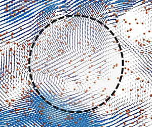
Although (3.12)–(3.14) are used conventionally for isotropic turbulence, the same definitions are applied for the unidirectional forcing cases (i.e. U256 and U384). Figure 1 shows some snapshots of the velocity field on the  $x$–
$x$– $y$ and $y$–
$y$– $z$ planes. Three-dimensional turbulent flows are confirmed for both the isotropic and unidirectional forcing cases. According to Yeung, Sreenivasan & Pope (Reference Yeung, Sreenivasan and Pope2018), the resolution $\eta /\Delta x=0.5$ is adequate for low-order statistics. Although the second-order centred finite difference is used in the present study, the values of $\eta /\Delta x$ are larger than 0.5 for all the cases. The effect of the grid resolution is assessed in Appendix A.

Figure 1. Velocity vector for (a,b) case I256, and (c,d) case U256 on (a,c) the  $x$–
$x$– $y$ plane, and (b,d) the $y$–
$y$– $z$ plane.
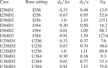
Table 2 shows the numerical conditions for particle-laden turbulence. To study the effect of the particle inertia, particles with three kinds of diameters (distinguished as D1, D2 and D3) are added to the base settings in table 1. The particle density is  $\rho _p=1000\rho _c$, and the dispersed phase volume fraction in the whole domain is $1.0\times 10^{-4}$ for all cases; for example, the numbers of particles in I256D1 and I256D3 are 85 921 and 3182, respectively. The Stokes number ${St}_K$ is defined by
 \begin{equation} {St}_K=\frac{\tau_p}{\tau_K}, \end{equation}
where  $\tau _p$ is the particle relaxation time scale,
 \begin{equation} \tau_p=\frac{\rho_p d_p^{2}}{18\rho_c\nu}, \end{equation}
and  $\tau _K$ is the Kolmogorov time scale,
 \begin{equation} {\tau_K}=\sqrt{\frac{\nu}{\epsilon}}. \end{equation}
The variables  $\eta$ and ${\tau _K}$ are based on the corresponding results for the single-phase turbulence, and ${St}_K$ is related directly to the particle size; a case with a larger diameter shows a larger ${St}_K$ value (see table 2). The particle diameter is comparable to the Kolmogorov length scale. The corresponding range of ${St}_K$ is up to $O(10^{2})$, which is larger than in the previous study (Moreau et al. Reference Moreau, Simonin and Bédat2010).
Table 2. Numerical condition for particle-laden turbulence. The base setting indicates the number of grid cells and the forcing condition in table 1.
4. Energy spectrum of particle-laden turbulence
The energy spectrum is defined as
 \begin{equation} E(|\boldsymbol{k}|)=E_x+E_y+E_z, \end{equation}
with an energy component  $E_i$ in each direction of the following form:
 \begin{equation} E_i(|\boldsymbol{k}|)=\int_{S(|\boldsymbol{k}|)} \tfrac{1}{2}\,\widehat{u_i}(\boldsymbol{k})\,\widehat{u_i}^{*}(\boldsymbol{k})\,{\rm d}S\quad \text{(no summation for}\ i), \end{equation}
where the superscript  $*$ indicates the complex conjugate, $\hat {\boldsymbol {u}}(\boldsymbol {k})$ is the Fourier-transformed velocity, and $S(|\boldsymbol {k}|)$ is the surface of the sphere of radius $|\boldsymbol {k}|$. Figure 2 shows $E$ and $E_i$ for two isotropic forcing cases with and without particles (I256 and I256D2). The isotropy is confirmed as $E_x$, $E_y$ and $E_z$ almost overlap with each other. In the case I256D2, $E$ is slightly smaller for $10 <|\boldsymbol {k}|/k_0 < 50$, whereas $E$ is larger for $|\boldsymbol {k}|/k_0 > 70$ compared with the case I256. This pivoting effect owing to the particles was observed in many studies (Elghobashi & Truesdell Reference Elghobashi and Truesdell1993; Sundaram & Collins Reference Sundaram and Collins1999; Boivin et al. Reference Boivin, Simonin and Squires2013). The dispersed particles interact locally with the fluid and influence directly the energy spectrum in the high wavenumber region (Schneiders et al. Reference Schneiders, Meinke and Schröder2017), leading to the increase in $E$. As the particles absorb energy from the large-scale eddies (Sundaram & Collins Reference Sundaram and Collins1999), $E$ decreases in the low wavenumber region. The enhanced energy dissipation in the high wavenumber region also attenuates the large-scale eddies.
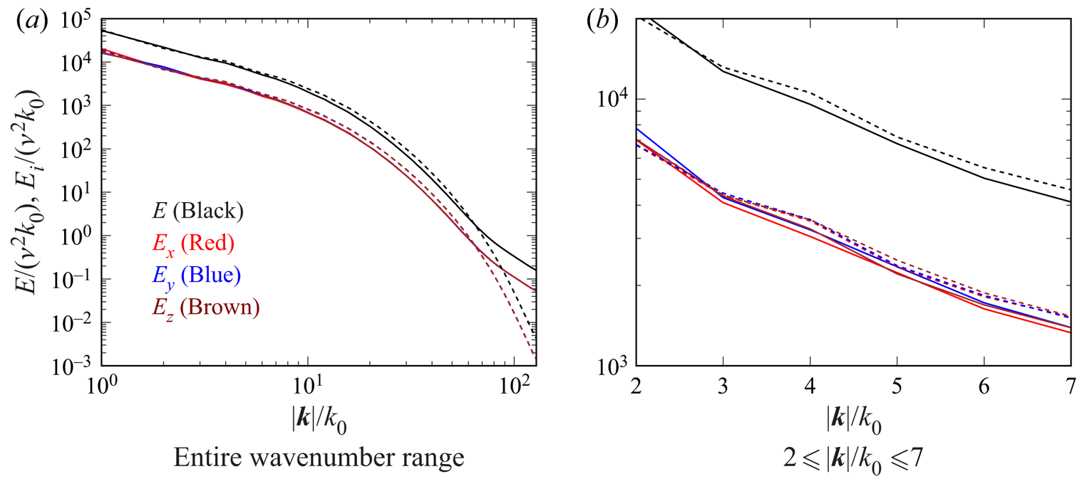
Figure 2. Energy spectra of isotropic turbulence. A solid line represents case I256D2, and a dashed line represents case I256. The energy spectrum  $E$ and the components are indicated by different colours.
Figure 3 shows  $E$ and $E_i$ for the anisotropic forcing case (U256D2). In contrast to the isotropic forcing cases (figure 2), there are clear differences in $E_x$, $E_y$ and $E_z$. As the unidirectional external force is in the $x$ direction (3.11), the component $E_x$ is larger than the other two components for the low wavenumber region ( $|\boldsymbol {k}|/k_0 < 5$). The second largest component at the lowest wavenumber $|\boldsymbol {k}|/k_0=1$ is $E_y$, indicating the formation of a large vortex of the axis parallel to the $z$ direction owing to the non-zero ${\rm d}U_x/{{\rm d} y}$, where $U_x$ is the $x$-component of the time-averaged fluid velocity. In the wavenumber range $|\boldsymbol {k}|/k_0\geqslant 2$, the effect of vortices perpendicular to the $z$ direction appears as $E_z$ larger than $E_y$. This difference in the vortical direction with respect to the wavenumber is consistent with the observation that the vortices on two adjacent scales tend to align at perpendicular angles to each other (Goto Reference Goto2008). The energy levels of $E_x$, $E_y$ and $E_z$ for the case U256D2 can be summarised as follows: $E_y < E_z\approx E_x$ in the wavenumber region $5\leqslant |\boldsymbol {k}|/k_0\leqslant 7$, and $E_y \approx E_z < E_x$ in the large wavenumber region ( $|\boldsymbol {k}|/k_0\geqslant 50$).

Figure 3. Energy spectra of anisotropic turbulence for case U256D2. The energy spectrum  $E$ and the components are indicated by different colours.
Figure 4 compares  $E$ for two forcing conditions (I256D2 and U256D2). Although the energy levels are similar at $|\boldsymbol {k}|/k_0=1$, the reduction of $E$ for high $|\boldsymbol {k}|/k_0$ $({>}20)$ is more significant for the case U256D2. Therefore, the energy ratio between the scales becomes larger for the unidirectional forcing case, indicating that the flow at $|\boldsymbol {k}|/k_0=1$ is intensified relatively by the energy input as the velocity profile tends to be aligned in the forcing direction, in comparison to the flow of the higher $|\boldsymbol {k}|/k_0$ region.
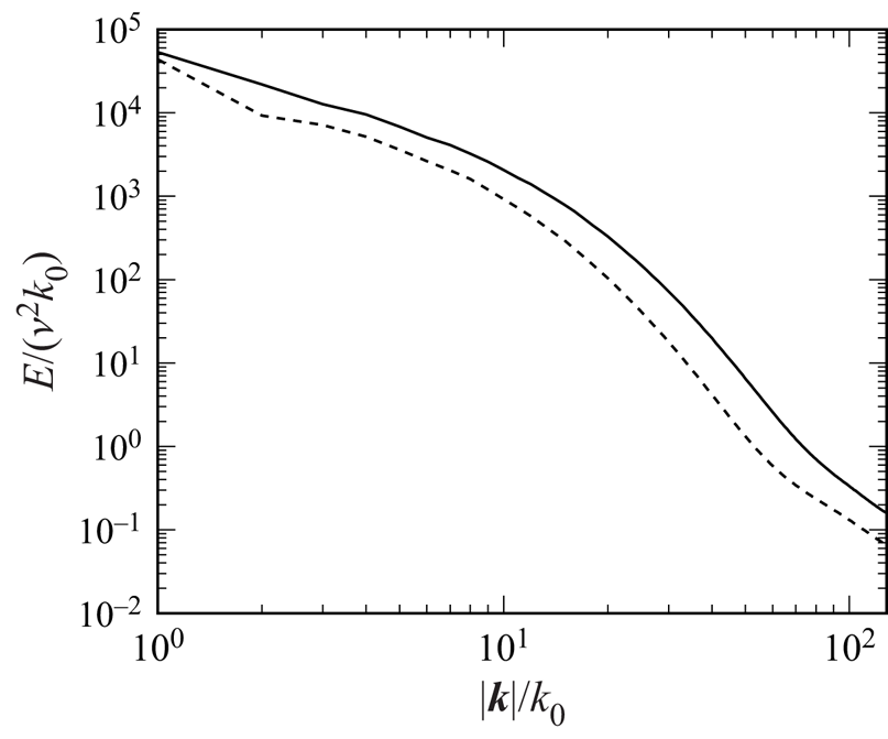
Figure 4. Energy spectra of isotropic and anisotropic turbulences. The solid line represents case I256D2, and the dashed line represents case U256D2.
5. Particle stress
5.1. Models of particle stress
To extract the effect of the direction of the particle stress tensor  $\boldsymbol {\tau }_{d}$, the deviatoric and isotropic parts are compared individually with their corresponding models. The isotropic and deviatoric parts of the tensors are denoted by the subscripts ‘iso’ and ‘dev’, respectively; for example, the particle stress $\boldsymbol {\tau }_{d}$ obtained by DNS is decomposed into
 $$\begin{gather} \boldsymbol{\tau}_{d,{iso}}=\tfrac{1}{3}\left({\rm tr}\,\boldsymbol{\tau}_d\right){\boldsymbol{\mathsf{I}}}, \end{gather}$$
 $$\begin{gather}\boldsymbol{\tau}_{d,{dev}}=\boldsymbol{\tau}_{d}-\boldsymbol{\tau}_{d,{iso}}, \end{gather}$$
where  ${\boldsymbol{\mathsf{I}}}$ is the identity tensor.
The fluid residual stress is regarded as the particle stress model as the particles receive the fluid force in the direction of decreasing relative velocities to the fluid. The particle Smagorinsky model and the particle scale-similarity model are also introduced as models that represent implicitly the effect of the fluid motion. The fluid residual stress model for the dispersed phase  $\boldsymbol {\tau }_d^{f}$ is given by $\boldsymbol {\tau }_c$ of (2.12) as
 \begin{equation} \boldsymbol{\tau}_d^{f}=\boldsymbol{\tau}_c; \end{equation}
the particle Smagorinsky model is only the deviatoric component as
 \begin{equation} \boldsymbol{\tau}_{d}^{pS}=\boldsymbol{\tau}_{d,{dev}}^{pS} ={-}(2R)^{2}|{\boldsymbol{\mathsf{S}}}_p|{\boldsymbol{\mathsf{S}}}_p, \end{equation}
where  $R$ is the radius of the averaging volume $V$, with
 $$\begin{gather} {\boldsymbol{\mathsf{S}}}_p=\boldsymbol{\nabla}\langle\boldsymbol{w}\rangle_d+ \left(\boldsymbol{\nabla}\langle\boldsymbol{w}\rangle_d\right)^{\rm T}- \tfrac{2}{3}\left(\boldsymbol{\nabla}\boldsymbol{\cdot}\langle\boldsymbol{w} \rangle_d\right){\boldsymbol{\mathsf{I}}}, \end{gather}$$
 $$\begin{gather}|{\boldsymbol{\mathsf{S}}}_p|=\sqrt{\tfrac{1}{2}{\boldsymbol{\mathsf{S}}}_p\colon{\boldsymbol{\mathsf{S}}}_p}; \end{gather}$$
and the particle scale-similarity model is
 \begin{equation} \boldsymbol{\tau}_d^{pB}= \left( \left\langle\left\langle \boldsymbol{w}\right\rangle_d\left\langle\boldsymbol{w}\right\rangle_d\right\rangle_d -\left\langle\left\langle \boldsymbol{w}\right\rangle_d\right\rangle_d\left\langle\left\langle \boldsymbol{w}\right\rangle_d\right\rangle_d \right). \end{equation}
The models  $\boldsymbol {\tau }_d^{pS}$ and $\boldsymbol {\tau }_d^{pB}$ are the counterparts of the models for the single-phase turbulence (Smagorinsky Reference Smagorinsky1963; Bardina, Ferziqer & Reynolds Reference Bardina, Ferziqer and Reynolds1983). For the isotropic part, we use the model introduced by Moreau et al. (Reference Moreau, Simonin and Bédat2010):
 \begin{equation} \boldsymbol{\tau}_{d}^{pY}=\boldsymbol{\tau}_{d,{iso}}^{pY}= (2R)^{2}|{\boldsymbol{\mathsf{S}}}_p|^{2}{\boldsymbol{\mathsf{I}}}. \end{equation}
The models  $\boldsymbol {\tau }_{d,{iso}}^{pB}=(1/3)({\rm tr}\,\boldsymbol {\tau }_d^{pB}){\boldsymbol{\mathsf{I}}}$ and $\boldsymbol {\tau }_{d,{iso}}^{pY}$ for the isotropic part of the particle stress are similar as both represent the fluctuation intensity of the particle velocity at the scale larger than $R$. Note that $\boldsymbol {\nabla }\langle \boldsymbol {w}\rangle _d$ is determined uniquely as long as $\alpha _d>0$ because the derivatives of $\alpha _d$ and $\alpha _d\left \langle \boldsymbol {w}\right \rangle _d$ are well-defined (Fukada et al. Reference Fukada, Fornari, Brandt, Takeuchi and Kajishima2018). However, $\left \langle \boldsymbol {w}\right \rangle _d$ is the $C^{1}$ function, and the evaluation of $\boldsymbol {\nabla }\langle \boldsymbol {w}\rangle _d$ requires a spatial resolution that is finer than the averaging volume, which is not adequate practically. Therefore, the gradient $\boldsymbol {\nabla }$ in (5.5) is replaced with a discretisation operator $\tilde {\boldsymbol {\nabla }}$, and the particle Smagorinsky model relates the smoothed velocity fluctuation at the grid scale and the particle stress. The discretisation operator $\tilde {\boldsymbol {\nabla }}=(\tilde {\partial }_x,\tilde {\partial }_y,\tilde {\partial }_z)$ is defined as
 \begin{equation} \tilde{\partial}_i \langle\boldsymbol{w}\rangle_d=\frac{-\left\langle\boldsymbol{w}\right\rangle_d (\boldsymbol{x}-(1/2)\,\Delta X\, \boldsymbol{e}_i)+\left\langle\boldsymbol{w}\right\rangle_d (\boldsymbol{x}+(1/2)\,\Delta X\,\boldsymbol{e}_i)}{\Delta X}, \end{equation}
where  $i$ is $x$,
$x$,  $y$ or $z$, and $\boldsymbol {e}_i$ the unit vector in the $i$ direction. The average represented by the outer brackets in the particle scale-similarity model (5.7) is computed with the values at the seven points $\boldsymbol {x}\pm (1/2)\,\Delta X\,\boldsymbol {e}_x$, $\boldsymbol {x}\pm (1/2)\,\Delta X\,\boldsymbol {e}_y$, $\boldsymbol {x}\pm (1/2)\,\Delta X\,\boldsymbol {e}_z$ and $\boldsymbol {x}$. The value of $\left \langle \boldsymbol {w}\right \rangle _d$ in (5.7) and (5.9) is computed directly from the numerical results.
The particle stress models are used by multiplying model coefficients  $C$ with the corresponding subscript and superscript:
 $$\begin{gather} C^{pS}_{dev}\boldsymbol{\tau}_{d,{dev}}^{pS}, \quad C^{pB}_{dev}\boldsymbol{\tau}_{d,{dev}}^{pB}, \quad C^{f}_{dev}\boldsymbol{\tau}_{d,{dev}}^{f}, \end{gather}$$
 $$\begin{gather}C^{pY}_{iso}\boldsymbol{\tau}_{d,{iso}}^{pY}, \quad C^{pB}_{iso}\boldsymbol{\tau}_{d,{iso}}^{pB}, \quad C^{f}_{iso}\boldsymbol{\tau}_{d,{iso}}^{f}. \end{gather}$$
As the model coefficient  $C^{pS}_{dev}$ is affected by the particle relaxation time and the time scale of the flow, $C^{pS}_{dev}$ is not a constant, in contrast to the Smagorinsky model for the single-phase turbulence. Although practical simulations require modelling of $\boldsymbol {\tau }_c$, the exact value of $\boldsymbol {\tau }_c$ obtained from the two-way coupling DNS result is used in the present study to focus on the relation between the particle and fluid unresolved motions. To compute the particle stress models in the two-way coupling DNS framework, the radius of the averaging volume $R$ and the virtual grid spacing $\Delta X$ need to be determined. For a large $R$ case, even though ${St}_K$ is larger than 1, the motion of the particles depends on the flow at the averaging scale. To investigate the effect of the flow at a scale larger than $\eta$, relatively large averaging volumes of $R/\eta =O(10)$ are considered, although this scale is not sufficient for a practical LES. The following $R$ values are employed: $k_0 R=0.75$, $1.13$ and $1.50$ (correspondingly, $R/\eta =44$, $66$ and $87$ for the case I256; see also $k_0\eta$ values in table 1). For each $k_0 R$ in each simulation condition, we compare the fully resolved particle stresses and their models at $20\,000$ different combinations of $\boldsymbol {x}$ and $t$.
$t$.
Figure 5 shows the influence of  $\Delta X$ on $\tilde {\partial }_x \langle w_x\rangle _d$ and $\tilde {\partial }_x \langle w_y\rangle _d$ along a line in the $x$ direction for the case of the smallest number of particles (I256D3) and the smallest averaging volume ( $k_0R=0.75$). The intensity of the fluctuation is remarkably large for the smallest $\Delta X/R$ ( ${=}\sqrt {3}/6$), while the intensity is suppressed and similar trends are obtained for the other cases ( $\Delta X/R=2\sqrt {3}/3$ and $\sqrt {3}$). In the present study, $\Delta X/R$ is set to be $2\sqrt {3}/3$ to reflect the collective motion of the particles that is not sensitive to small random disturbances.

Figure 5. Components of discretised gradient (a)  $\tilde {\partial }_x\langle w_x\rangle _d$ and (b) $\tilde {\partial }_x\langle w_y\rangle _d$, along a line parallel to the $x$-axis, for the case I256D3 with $k_0 R=0.75$.
To compare the roles of  $\boldsymbol {\tau }_{d,{iso}}$ and $\boldsymbol {\tau }_{d,{dev}}$, the energy transfer of the dispersed phase between the grid scale and the subgrid scale is studied. By multiplying (2.6) by $\left \langle \boldsymbol {w}\right \rangle _d$, we obtain the equation corresponding to the energy transport of the dispersed phase at the grid scale:
 \begin{align} &\frac{\partial}{\partial t}\left(\frac{1}{2}\,\alpha_d\left\langle\boldsymbol{w}\right\rangle_d \boldsymbol{\cdot}\left\langle\boldsymbol{w}\right\rangle_d\right) +\boldsymbol{\nabla}\boldsymbol{\cdot}\left\{\frac{1}{2}\,\alpha_d\left\langle \boldsymbol{w}\right\rangle_d\left(\left\langle\boldsymbol{w}\right\rangle_d \boldsymbol{\cdot}\left\langle\boldsymbol{w}\right\rangle_d\right)\right\}\nonumber\\ &\quad ={-}\boldsymbol{\nabla}\boldsymbol{\cdot}\left(\alpha_d \boldsymbol{\tau}_d\boldsymbol{\cdot}\left\langle\boldsymbol{w}\right\rangle_d\right) +\alpha_d\boldsymbol{\tau}_d\colon\boldsymbol{\nabla}\langle\boldsymbol{w}\rangle_d +\boldsymbol{F}\boldsymbol{\cdot}\left\langle\boldsymbol{w}\right\rangle_d+ \alpha_d\boldsymbol{g}_d\boldsymbol{\cdot}\left\langle\boldsymbol{w}\right\rangle_d, \end{align}
where the second term of the right-hand side is the energy transfer between the scales owing to the particle stress. This energy transfer term is decomposed as
 \begin{equation} \boldsymbol{\tau}_d\colon\tilde{\boldsymbol{\nabla}}\langle\boldsymbol{w}\rangle_d= \boldsymbol{\tau}_{d,{iso}}\colon\tilde{\boldsymbol{\nabla}}\langle\boldsymbol{w}\rangle_d +\boldsymbol{\tau}_{d,{dev}}\colon\tilde{\boldsymbol{\nabla}}\langle\boldsymbol{w}\rangle_d, \end{equation}
where the gradient is replaced by  $\tilde {\boldsymbol {\nabla }}=(\tilde {\partial }_x,\tilde {\partial }_y,\tilde {\partial }_z)$ defined by (5.9), and $\alpha _d$ is omitted. Figure 6 shows the p.d.f.s of $\boldsymbol {\tau }_d\colon \tilde {\boldsymbol {\nabla }}\left \langle \boldsymbol {w}\right \rangle _d$, $\boldsymbol {\tau }_{d,{iso}}\colon \tilde {\boldsymbol {\nabla }}\left \langle \boldsymbol {w}\right \rangle _d$ and $\boldsymbol {\tau }_{d,{dev}}\colon \tilde {\boldsymbol {\nabla }}\left \langle \boldsymbol {w}\right \rangle _d$ for the case I256D2 and $k_0 R=1.13$. As the magnitudes of the isotropic and deviatoric contributions are comparable, the particle stress models of both parts are important. The energy transfer corresponding to the isotropic part $\boldsymbol {\tau }_{d,{iso}}\colon \tilde {\boldsymbol {\nabla }}\left \langle \boldsymbol {w}\right \rangle _d$ is related to the divergence $\tilde {\boldsymbol {\nabla }}\boldsymbol {\cdot }\left \langle \boldsymbol {w}\right \rangle _d$; the p.d.f. of $\boldsymbol {\tau }_{d,{iso}}\colon \tilde {\boldsymbol {\nabla }}\left \langle \boldsymbol {w}\right \rangle _d/\epsilon$ takes a symmetric distribution centred at 0, although this is caused by a mechanism that is different from the divergence-free condition of the incompressible flow. The contribution of the deviatoric part $\boldsymbol {\tau }_{d,{dev}}\colon \tilde {\boldsymbol {\nabla }}\left \langle \boldsymbol {w}\right \rangle _d$ tends to have a negative value, and the sum of both contributions has a higher probability of being a negative value, meaning that the energy is transferred from the grid scale to the subgrid scale. Therefore, the particle stress model for the deviatoric part is important for the prediction of the net energy transfer.
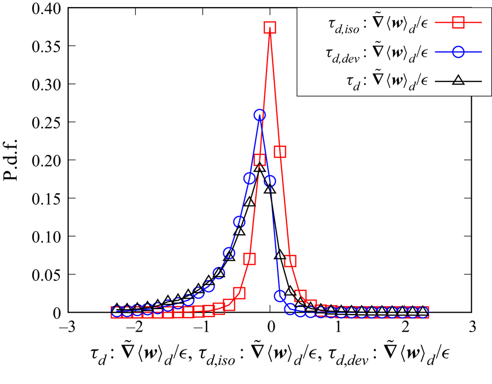
Figure 6. P.d.f.s of the energy transfer of the dispersed phase  $\boldsymbol {\tau }_d\colon \tilde {\boldsymbol {\nabla }}\left \langle \boldsymbol {w}\right \rangle _d$ and the components $\boldsymbol {\tau }_{d,{iso}}\colon \tilde {\boldsymbol {\nabla }}\left \langle \boldsymbol {w}\right \rangle _d$ and $\boldsymbol {\tau }_{d,{dev}}\colon \tilde {\boldsymbol {\nabla }}\left \langle \boldsymbol {w}\right \rangle _d$ for the case I256D2 with $k_0 R=1.13$.
5.2. Principal axes of the particle stress
The agreement of the principal axes (APA) of the particle stress models with those of the fully resolved particle stress is important to predict the sign of the energy transfer term. The eigenvalues of the tensor  $\boldsymbol {\tau }$ are denoted as $\lambda _{\alpha }(\boldsymbol {\tau })$, $\lambda _{\beta }(\boldsymbol {\tau })$ and $\lambda _{\gamma }(\boldsymbol {\tau })$, and the corresponding eigenvectors (principal axes) are $\boldsymbol {e}_{\alpha }(\boldsymbol {\tau })$, $\boldsymbol {e}_{\beta }(\boldsymbol {\tau })$ and $\boldsymbol {e}_{\gamma }(\boldsymbol {\tau })$, respectively. The eigenvalues and eigenvectors are distinguished by $\lambda _{\alpha } > \lambda _{\beta } > \lambda _{\gamma }$; a case of two identical eigenvalues does not occur in this study. A degree of APA is given by the following direction cosines:
 $$\begin{gather} \cos\theta_{\alpha}=\left|\boldsymbol{e}_{\alpha}(\boldsymbol{\tau}_{d,{ dev}})\boldsymbol{\cdot}\boldsymbol{e}_{\alpha}(\boldsymbol{\tau}_{d,{dev}}^{model})\right|, \end{gather}$$
 $$\begin{gather}\cos\theta_{\beta}=\left|\boldsymbol{e}_{\beta}(\boldsymbol{\tau}_{d,{ dev}})\boldsymbol{\cdot}\boldsymbol{e}_{\beta}(\boldsymbol{\tau}_{d,{dev}}^{ model})\right|, \end{gather}$$
 $$\begin{gather}\cos\theta_{\gamma}=\left|\boldsymbol{e}_{\gamma}(\boldsymbol{\tau}_{d,{ dev}})\boldsymbol{\cdot}\boldsymbol{e}_{\gamma}(\boldsymbol{\tau}_{d,{dev}}^{ model})\right|, \end{gather}$$
where  $\boldsymbol {\tau }_d$ is the particle stress based on the two-way coupling DNS results, and $\boldsymbol {\tau }_{d,{dev}}^{model}$ corresponds to $\boldsymbol {\tau }_{d,{dev}}^{f}$, $\boldsymbol {\tau }_{d,{dev}}^{pS}$ and $\boldsymbol {\tau }_{d,{dev}}^{pB}$. Although the eigenvectors may have opposite directions (e.g. $-\boldsymbol {e}_{\alpha }$ instead of $\boldsymbol {e}_{\alpha }$), these two directions have no substantial difference. Therefore, the absolute values are employed in (5.14)–(5.16).
Another degree of APA is assessed by using the quaternion. By a rotation of the coordinates, three eigenvectors  $\boldsymbol {e}_{\alpha }(\boldsymbol {\tau }_{d,{dev}}^{model})$, $\boldsymbol {e}_{\beta }(\boldsymbol {\tau }_{d,{dev}}^{model})$ and $\boldsymbol {e}_{\gamma }(\boldsymbol {\tau }_{d,{dev}}^{model})$ can be transformed to $\boldsymbol {e}_{\alpha }(\boldsymbol {\tau }_{d,{dev}})$, $\boldsymbol {e}_{\beta }(\boldsymbol {\tau }_{d,{dev}})$ and $\boldsymbol {e}_{\gamma }(\boldsymbol {\tau }_{d,{dev}})$, respectively. The rotation is quantified by the quaternion
 \begin{equation} q(\boldsymbol{\tau}_{d,{dev}},\boldsymbol{\tau}_{d,{dev}}^{ model})=\cos\frac{\theta_q}{2}+ia_1\sin\frac{\theta_q}{2}+ ja_2\sin\frac{\theta_q}{2}+ka_3\sin\frac{\theta_q}{2}, \end{equation}
where  $\boldsymbol {a}=(a_1,a_2,a_3)$ is the rotation axis, $\theta _q$ is the rotation angle, and $i$,
$i$,  $j$ and $k$ are the imaginary units of the algebra of quaternions (Farebrother, Groß & Troschke Reference Farebrother, Groß and Troschke2003). By determining $q(\boldsymbol {\tau }_{d,{dev}},\boldsymbol {\tau }_{d,{dev}}^{model})$, $\cos \theta _q$ can represent a degree of APA between $\boldsymbol {\tau }_{d,{dev}}$ and $\boldsymbol {\tau }_{d,{ dev}}^{model}$; a value close to 1 indicates a good agreement of the predicted particle stress field. As $q(\boldsymbol {\tau }_{d,{ dev}},\boldsymbol {\tau }_{d,{dev}}^{model})$ and corresponding $\theta _q$ are not unique (e.g. $q$ and $-q$ indicate the same rotation, and the corresponding $\theta _q$ are different), we take the smallest positive $\theta _q$ among all possible values.
Figures 7–9 show the profiles of the p.d.f.s of  $\cos \theta _{\alpha }$, $\cos \theta _{\beta }$ and $\cos \theta _{\gamma }$ for the three stress models. The results for the cases I256D1, U256D1, I256D3 and U256D3 are shown to compare the effects of the isotropy of the external forces and ${St}_K$. For the eigenvector $\boldsymbol {e}_{\alpha }$ (figure 7), the high probabilities are observed in the range $\cos \theta _{\alpha }>0.9$ for $\boldsymbol {\tau }_{d,{dev}}^{pB}$ and $\boldsymbol {\tau }_{d,{ dev}}^{f}$ of all four cases of isotropic/anisotropic forcing with small/large particle diameters. As the probabilities of $\cos \theta _{\alpha }>0.9$ for $\boldsymbol {\tau }_{d,{dev}}^{pB}$ are larger than those for $\boldsymbol {\tau }_{d,{dev}}^{f}$, the scale-similarity assumption is effective to predict the principal axis of the largest eigenvalue $\lambda _{\alpha }$. For the particle Smagorinsky model $\boldsymbol {\tau }_{d,{dev}}^{pS}$, the largest probability takes place at approximately $\cos \theta _{\alpha }=0.8$ for the unidirectional forcing cases (figures 7b,d), unlike the other two particle stress models. For the isotropic forcing cases (figures 7a,c), the probabilities of $\cos \theta _{\alpha }>0.9$ for $\boldsymbol {\tau }_{d,{dev}}^{pB}$ and $\boldsymbol {\tau }_{d,{dev}}^{f}$ tend to decrease with ${St}_K$ (i.e. with larger particle diameters), whereas the probabilities for $\boldsymbol {\tau }_{d,{dev}}^{pS}$ remain at approximately the same level regardless of ${St}_K$, indicating the difference in the characteristics of the models with ${St}_K$.

Figure 7. P.d.f.s of  $\cos \theta _{\alpha }$: (a) I256D1, (b) U256D1, (c) I256D3, (d) U256D3. The particle stress models are indicated by different colours. The sizes of the averaging volumes are indicated by different symbols.
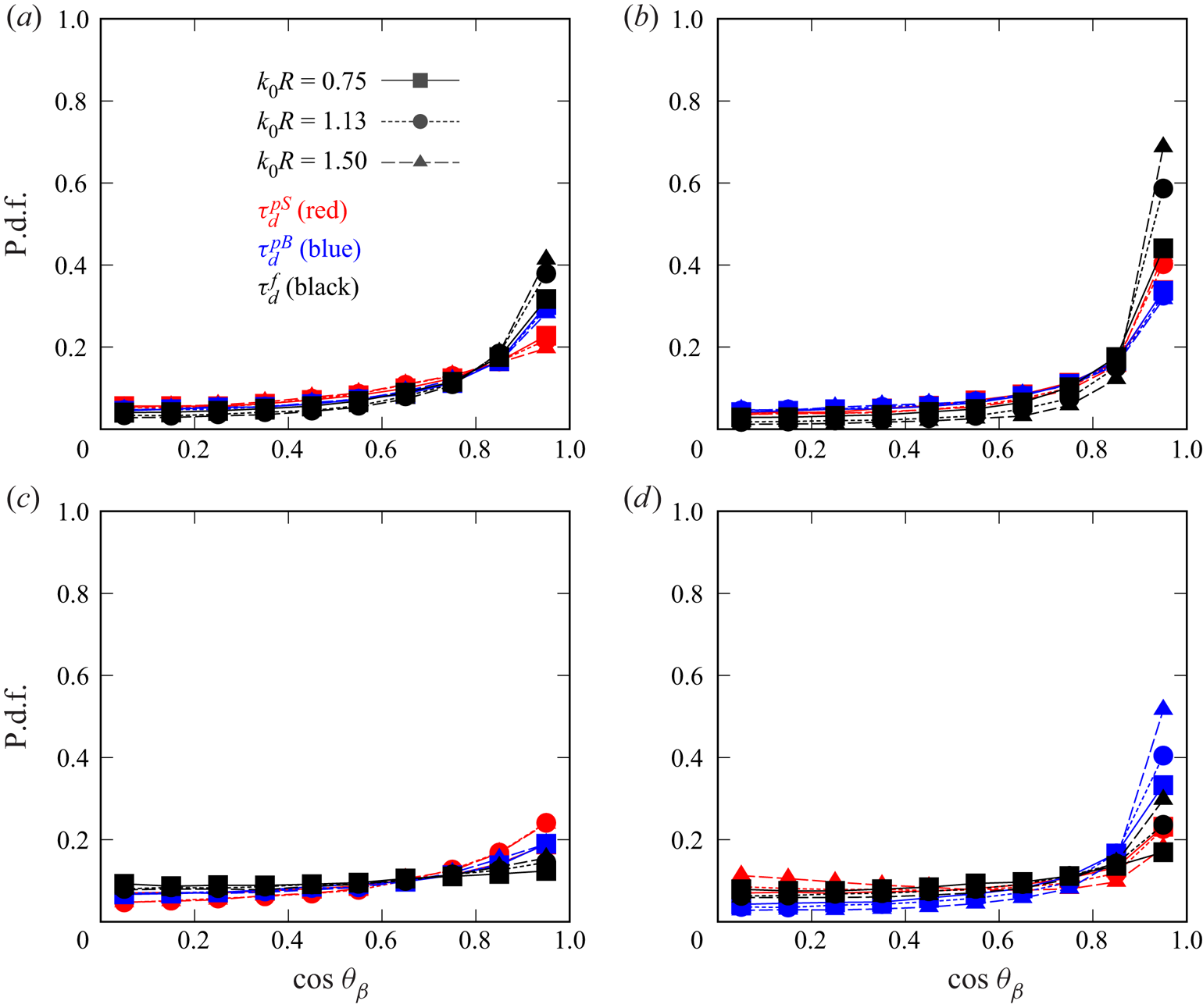
Figure 8. P.d.f.s of  $\cos \theta _{\beta }$: (a) I256D1, (b) U256D1, (c) I256D3, (d) U256D3. The particle stress models are indicated by different colours. The sizes of the averaging volumes are indicated by different symbols.

Figure 9. P.d.f.s of  $\cos \theta _{\gamma }$: (a) I256D1, (b) U256D1, (c) I256D3, (d) U256D3. The particle stress models are indicated by different colours. The sizes of the averaging volumes are indicated by different symbols.
The trends of  $\cos \theta _{\beta }$ and $\cos \theta _{\gamma }$ (figures 8 and 9) are similar to each other in some aspects, as explained below. The probabilities of $\cos \theta _{\beta }>0.9$ and $\cos \theta _{\gamma }>0.9$ for $\boldsymbol {\tau }_{d,{dev}}^{f}$ are larger than those for $\boldsymbol {\tau }_{d,{dev}}^{pB}$ at the small ${St}_K$ cases (figures 8a,b and 9a,b), and the advantage of the scale-similarity model observed in figure 7 no longer exists. For the large ${St}_K$ case under the isotropic forcing condition (figures 8c and 9c), the probabilities for $\boldsymbol {\tau }_{d,{dev}}^{pS}$ are higher than those of $\boldsymbol {\tau }_{d,{dev}}^{pB}$ and $\boldsymbol {\tau }_{d,{dev}}^{f}$. In addition, the difference in the trends of $\cos \theta _{\beta }$ and $\cos \theta _{\gamma }$ for $\boldsymbol {\tau }_{d,{dev}}^{pS}$ is confirmed for the unidirectional forcing cases (figures 8b,d and 9b,d); the maximum values of the probabilities are at around $\cos \theta _{\beta }=1$ and $\cos \theta _{\gamma }=0.7$.
The intensity of the fluid velocity fluctuation inside the averaging volume  $V$ is related to the radius $R$. The probabilities of $\cos \theta _{\alpha }>0.9$, $\cos \theta _{\beta }>0.9$ and $\cos \theta _{\gamma }>0.9$ for $\boldsymbol {\tau }_{d,{dev}}^{f}$ increase with $k_0R$ for all the cases (figures 7–9). Therefore, although the particle motions are different from the background flow around the individual particles, the motions are affected by the flow of scales close to $R$, and this effect enhances with the volume size.
Considering that the collective particle motion is influenced by the flow inside the averaging volume, and that the turbulence intensity varies in space, it is important to evaluate the models based on locally averaged information. The Stokes number reflecting the effect of local information in the averaging volume is defined as
 \begin{equation} {St}_R=\tau_p\,\frac{\epsilon}{u_R^{2}}, \end{equation}
where  $u_R^{2}$ is the fluctuation intensity of the fluid velocity inside the volume obtained by
 \begin{equation} u_R^{2}=\tfrac{1}{3}\,{\rm tr}\,\boldsymbol{\tau}_c, \end{equation}
and the dissipation rate is calculated as
 \begin{equation} \epsilon=\int |\boldsymbol{k}|^{2}\,E(|\boldsymbol{k}|)\,{\rm d}|\boldsymbol{k}| + \frac{1}{L_{cube}^{3}}\sum_{particles}\boldsymbol{f}\boldsymbol{\cdot} \alpha_s(\left\langle\boldsymbol{u}\right\rangle_s(\boldsymbol{x}_p)-\boldsymbol{w}_p). \end{equation}
The second term on the right-hand side of (5.20) indicates the unresolved dissipation in the vicinity of the particle surface. By analogy with the scale estimation of turbulence (Tennekes & Lumley Reference Tennekes and Lumley1972), the value  $u_R^{2}/\epsilon$ is considered as the time scale for dissipating the eddy of velocity $u_R$. Note that $\epsilon$ is the averaged value and that the effect of the averaging volume size is reflected in (5.18) through $u_R^{2}$ (e.g. $u_R^{2}\to 0$ for $R\to 0$). As an indicator similar to ${St}_R$, the locally defined time scale based on the strain rate and the eddy viscosity of LES was introduced as the model input for the particle acceleration in the Euler–Lagrangian framework (Gorokhovski & Zamansky Reference Gorokhovski and Zamansky2018). Using (5.18), the degree of APA based on the quaternion (5.17) is evaluated by the conditional probability $A_x({St}_R)$ of being $\cos \theta _q\geqslant x$ for a fixed ${St}_R$. A large value of $A_x$ indicates that the model describes accurately the particle stress field in terms of the degree of APA.
Figure 10 shows the conditional probability  $A_{0.8}$ for all the cases of the two-way coupling simulations. The values of $A_{0.8}$ for $\boldsymbol {\tau }_{d,{dev}}^{pS}$, $\boldsymbol {\tau }_{d,{dev}}^{pB}$ and $\boldsymbol {\tau }_{d,{ dev}}^{f}$ are regarded as the functions of ${St}_R$, and the different trends for the models are observed clearly. In particular, $\boldsymbol {\tau }_{d,{dev}}^{f}$ is predominant for ${St}_R<1$ for all the cases, which corresponds to the result for the small ${St}_K$ cases shown in figures 8(a), 8(b), 9(a) and 9(b). Bragg, Ireland & Collins (Reference Bragg, Ireland and Collins2015) showed theoretically that the particle motion is related to the fluid velocity gradient at scale $r$ if the Stokes number based on $r$ is smaller than 1; otherwise, the effect of the larger flow structure is dominant. This theoretical result coincides with the predominance of $\boldsymbol {\tau }_{d,{dev}}^{f}$ as the particle motion is affected by the flow structure at the scale $R$ for ${St}_R<1$. Note that although $R$ is much smaller than the upper limit of effective scales (e.g. the scale $O(10^{3})$ times $\eta$ for ${St}_K=0.1$; (Tom & Bragg Reference Tom and Bragg2019)) and the particles do not follow the subgrid fluid flow, the flow at the scale $R$ is still effective for the particle stress.

Figure 10. Degree of APA for the models to those for the fully resolved particle stress based on the quaternion  $\cos \theta _q$ against ${St}_R$ defined by (5.18): (a) I256D $X$, (b) U256D $X$, (c) I384D $X$, (d) U384D $X$, where D $X$ is D1, D2 or D3. The particle stress models are indicated by different colours: red, blue and black represent $\boldsymbol {\tau }_{d,{dev}}^{pS}$, $\boldsymbol {\tau }_{d,{dev}}^{pB}$ and $\boldsymbol {\tau }_{d,{dev}}^{f}$, respectively. The sizes of the averaging volume are indicated by different line types. The particle conditions (D $X$) are indicated by different symbols.
The conditional probability  $A_{0.8}$ for $\boldsymbol {\tau }_{d,{dev}}^{pB}$ is larger than that for $\boldsymbol {\tau }_{d,{dev}}^{f}$ for ${St}_R>5$ as $\boldsymbol {\tau }_{d,{dev}}^{pB}$ (related to the spatial variation of $\left \langle \boldsymbol {w}\right \rangle _d$) is related to the flow structure larger than $R$. For the isotropic forcing cases (figures 10a,c), $A_{0.8}$ for $\boldsymbol {\tau }_{d,{dev}}^{pB}$ decreases with increasing ${St}_R$. Considering the case that the $xx$-component of the particle stress is dominant owing to the positive and negative $w_{px}$ of the individual particles inside the averaging volume, the decreasing trend of $A_{0.8}$ for $\boldsymbol {\tau }_{d,{dev}}^{pB}$ is understood as $\left \langle w_x\right \rangle _d$, and its spatial variation can be almost zero regardless of the flow structure at the scale $R$ for large ${St}_R$.
For the unidirectional forcing cases, as already shown in figure 3,  $E_y< E_z\approx E_x$ for the low-wavenumber region and $E_y\approx E_z< E_x$ for the high-wavenumber region were observed, in contrast to the isotropic forcing cases where an equal distribution of energy was observed. This uneven distribution of $E_i$ suggests that the $zz$-component (related to $E_z$) of $\boldsymbol {\tau }_{d,{dev}}^{pB}$ estimated on the large scale tends to be large, while the predominance of this component is reduced for the particle subgrid stress $\boldsymbol {\tau }_{d,{dev}}$ for small ${St}_R$, indicating that $A_{0.8}$ for $\boldsymbol {\tau }_{d,{ dev}}^{pB}$ is suppressed. Therefore, $A_{0.8}$ for $\boldsymbol {\tau }_{d,{dev}}^{pB}$ does not exhibit a clear decreasing trend with increasing ${St}_R$ in the unidirectional forcing cases (figures 10b,d) in contrast to the isotropic forcing cases (figures 10a,c).
To examine the validity of using the averaged  $\epsilon$ for ${St}_R$ defined by (5.18), the above result for $A_{0.8}$ is compared with that defined with the local dissipation $\epsilon _{loc}$ inside $V$. The probability $A_{0.8}$ based on $\epsilon _{loc}$ in figure 11 shows similar but diffused profiles in comparison with that based on $\epsilon$ in figure 10, indicating that ${St}_R$ defined with $\epsilon$ is preferable to extract the particle stress behaviour. The energy loss of the flow inside $V$ is caused by the convective transport as well as the viscous dissipation, and the rate of the energy loss is different from $\epsilon _{loc}$. In the case that the energy is supplied from the outside to maintain the flow structure inside $V$, the lifetime of the flow structure becomes longer than the estimated value $u_R^{2}/\epsilon _{loc}$. Therefore, the locally defined $\epsilon _{loc}$ is not always adequate, and the mean value $\epsilon$ is employed for ${St}_R$ in this study.

Figure 11. Degree of APA for the models to those for the fully resolved particle stress based on the quaternion  $\cos \theta _q$ against ${St}_R$ based on $\epsilon _{loc}$: (a) I256D $X$, (b) U256D $X$, (c) I384D $X$, (d) U384D $X$, where D $X$ is D1, D2 or D3. The particle stress models are indicated by different colours: red, blue and black represent $\boldsymbol {\tau }_{d,{dev}}^{pS}$, $\boldsymbol {\tau }_{d,{dev}}^{pB}$ and $\boldsymbol {\tau }_{d,{dev}}^{f}$, respectively. The sizes of the averaging volume are indicated by different line types. The particle conditions (D $X$) are indicated by different symbols.
5.3. Correlation coefficient for the deviatoric part
To investigate the characteristics of the magnitudes (related to the eigenvectors) as well as the principal axes of the particle stress models, the correlation coefficient of the deviatoric part is defined as
 \begin{equation} D_{dev}({St}_R)=\frac{\displaystyle\sum\nolimits^{St_R} \delta\boldsymbol{\tau}_{d,{dev}}\colon\delta\boldsymbol{\tau}_{d,{dev}}^{model}} {\displaystyle\sqrt{\sum\nolimits^{St_R}\delta\boldsymbol{\tau}_{d,{dev}}\colon\delta\boldsymbol{\tau}_{d,{ dev}}} \sqrt{ \displaystyle\sum\nolimits^{St_R}\delta\boldsymbol{\tau}_{d,{ dev}}^{model}\colon\delta\boldsymbol{\tau}_{d,{dev}}^{ model}}}, \end{equation}
where  $\sum ^{{St}_R}$ indicates the summation at a fixed ${St}_R$ (hereafter, the conditional summation), and $\delta \boldsymbol {\tau }_{d,{dev}}$ and $\delta \boldsymbol {\tau }_{d,{dev}}^{model}$ are
 \begin{equation} \delta\boldsymbol{\tau}_{d,{dev}}=\boldsymbol{\tau}_{d,{dev}}- \frac{\displaystyle\sum\nolimits^{{St}_R} \boldsymbol{\tau}_{d,{ dev}}}{\displaystyle\sum\nolimits^{{St}_R} 1},\quad \delta\boldsymbol{\tau}_{d,{ dev}}^{model}=\boldsymbol{\tau}_{d,{dev}}^{ model}-\frac{\displaystyle\sum\nolimits^{{St}_R}\boldsymbol{\tau}_{d,{ dev}}^{model}}{\displaystyle\sum\nolimits^{{St}_R}1}, \end{equation}
respectively. Figure 12 compares the dependence of  $D_{dev}$ on ${St}_R$ for each model ( $\boldsymbol {\tau }_{d,{dev}}^{pS}$, $\boldsymbol {\tau }_{d,{dev}}^{pB}$ and $\boldsymbol {\tau }_{d,{dev}}^{f}$). The trend of $D_{dev}$ is similar to the degree of APA (figure 10) such that the models $\boldsymbol {\tau }_{d,{dev}}^{f}$ and $\boldsymbol {\tau }_{d,{ dev}}^{pB}$ show the highest and the second highest $D_{dev}$ for ${St}_R<1$, which also confirms the effectiveness of ${St}_R$ for extracting the characteristics of the particle stress in terms of the correlation coefficient. In general, by superposing a single vortex of the scale $R$ and disturbances, $\boldsymbol {\tau }_{d,{dev}}^{f}$ and $\boldsymbol {\tau }_{d,{iso}}^{f}$ reflect the structures of the scale $R$ and smaller scales, respectively. Therefore, the correlation coefficient $D_{dev}$ for the model $\boldsymbol {\tau }_{d,{dev}}^{f}$ is regarded as the contribution of the fluid motion of the scale $R$ for ${St}_R<1$. The differences between figures 10 and 12 are also observed; as $D_{dev}$ for $\boldsymbol {\tau }_{d,{dev}}^{pB}$ in the case U256D $X$ (
$X$ ( $X=1,2,3$; figure 12b) shows a slightly decreasing trend with increasing ${St}_R$ in contrast to the increasing trend of $A_{0.8}$ (figure 10b), the prediction of the magnitude of the particle stress by $\boldsymbol {\tau }_{d,{dev}}^{pB}$ is preferable for small ${St}_R$. For ${St}_R>5$, the $D_{dev}$ values for $\boldsymbol {\tau }_{d,{dev}}^{pS}$ are close to those for $\boldsymbol {\tau }_{d,{dev}}^{pB}$ for all the cases as $\boldsymbol {\tau }_{d,{dev}}^{pS}$ and $\boldsymbol {\tau }_{d,{ dev}}^{pB}$ are related to the similar fluctuation intensities of $\left \langle \boldsymbol {w}\right \rangle _d$ at the same scale larger than $R$.
$R$.

Figure 12. Correlation coefficients of the particle stress models for the deviatoric part  $D_{dev}$: (a) I256D $X$, (b) U256D $X$, (c) I384D $X$, (d) U384D $X$, where D $X$ is D1, D2 or D3. The particle stress models are indicated by different colours: red, blue and black represent $\boldsymbol {\tau }_{d,{dev}}^{pS}$, $\boldsymbol {\tau }_{d,{dev}}^{pB}$ and $\boldsymbol {\tau }_{d,{dev}}^{f}$, respectively. The sizes of the averaging volume are indicated by different line types. The particle conditions (D $X$) are indicated by different symbols.
In addition to  $D_{dev}$ as the direct evaluation of the particle stress model, the correlation coefficient of the energy transfer rate $\boldsymbol {\tau }_{d,{dev}}\colon \tilde {\boldsymbol {\nabla }}\langle \boldsymbol {w}\rangle _d$ is also defined as
 \begin{equation} H_{dev}({St}_R)=\frac{ \displaystyle\sum\nolimits^{{St}_R}\delta h_{ dev}\,\delta h_{dev}^{model}} {\sqrt{ \displaystyle\sum\nolimits^{{St}_R} \delta h_{dev}\,\delta h_{dev}} \sqrt{ \displaystyle\sum\nolimits^{{St}_R} \delta h_{dev}^{model}\,\delta h_{dev}^{model}}}, \end{equation}
where
 $$\begin{gather} \delta h_{dev}=\boldsymbol{\tau}_{d,{dev}}\colon\tilde{\boldsymbol{\nabla}} \langle\boldsymbol{w}\rangle_d- \left.\sum\nolimits^{{St}_R} \boldsymbol{\tau}_{d,{dev}}\colon\tilde{\boldsymbol{\nabla}}\langle \boldsymbol{w}\rangle_d\right/\sum\nolimits^{{St}_R}1, \end{gather}$$
 $$\begin{gather}\delta h_{dev}^{model}=\boldsymbol{\tau}_{d,{dev}}^{model}\colon\tilde{\boldsymbol{\nabla}}\langle\boldsymbol{w}\rangle_d- \left.\sum\nolimits^{{St}_R}\boldsymbol{\tau}_{d,{dev}}^{ model}\colon\tilde{\boldsymbol{\nabla}}\langle\boldsymbol{w} \rangle_d\right/\sum\nolimits^{{St}_R}1. \end{gather}$$
Figure 13 shows the dependence of  $H_{dev}$ on ${St}_R$ for each model. For the models $\boldsymbol {\tau }_{d,{dev}}^{pS}$ and $\boldsymbol {\tau }_{d,{dev}}^{pB}$ that are related to the fluctuation intensity of the particle velocity $\left \langle \boldsymbol {w}\right \rangle _d$, the values of $H_{dev}$ tend to be higher than those of $D_{dev}$ (figure 12). This tendency for $H_{dev}$ is consistent with the result of Moreau et al. (Reference Moreau, Simonin and Bédat2010). As a result, the models based on the particle velocity $\left \langle \boldsymbol {w}\right \rangle _d$ are preferable in the sense of the energy transfer rate ( $H_{dev}$) for the range ${St}_R>1$. For ${St}_R<1$, the model $\boldsymbol {\tau }_{d,{dev}}^{f}$ is predominant as well as the model $\boldsymbol {\tau }_{d,{dev}}^{pB}$ for the energy transfer rate.

Figure 13. Correlation coefficients of the energy transfer rate by the particle stress models for the deviatoric part  $H_{dev}$: (a) I256D $X$, (b) U256D $X$, (c) I384D $X$, (d) U384D $X$, where D $X$ is D1, D2 or D3. The particle stress models are indicated by different colours: red, blue and black represent $\boldsymbol {\tau }_{d,{dev}}^{pS}$, $\boldsymbol {\tau }_{d,{dev}}^{pB}$ and $\boldsymbol {\tau }_{d,{dev}}^{f}$, respectively. The sizes of the averaging volume are indicated by different line types. The particle conditions (D $X$) are indicated by different symbols.
5.4. Correlation coefficient for the isotropic part
By replacing the subscript ‘dev’ with ‘iso’ in (5.21) and (5.22a,b), the correlation coefficient of the isotropic part  $D_{iso}$ is investigated. Figure 14 shows $D_{iso}$ for the models $\boldsymbol {\tau }_{d,{iso}}^{pY}$ and $\boldsymbol {\tau }_{d,{iso}}^{pB}$. As ${St}_R$ is fixed for the conditional summation, $\boldsymbol {\tau }_{d,{iso}}^{f}=(\epsilon \tau _p/{St}_R){\boldsymbol{\mathsf{I}}}$ takes a constant component in the diagonals, and therefore $D_{iso}$ for $\boldsymbol {\tau }_{d,{iso}}^{f}$ is not defined. The correlation coefficient depends largely on the averaging volume and ${St}_K$, and the differences of the $D_{iso}$ distributions between the models are not as clear as observed in figure 12. In the scale-similarity model, the unresolved particle stress is extrapolated from the resolved scale and the effect of scales that are much smaller than $R$ is not predicted accurately, while the effect of the small scales is relatively weak for the deviatoric part. Therefore, even for ${St}_R<1$, $D_{iso}$ for $\boldsymbol {\tau }_{d,{iso}}^{pB}$ is not as high as $D_{dev}$ (figure 12) for all the cases. The model $\boldsymbol {\tau }_{d,{iso}}^{pY}$ is more effective than $\boldsymbol {\tau }_{d,{iso}}^{pB}$ for ${St}_R<1$ in the sense of the correlation coefficient $D_{iso}$.

Figure 14. Correlation coefficients of the particle stress models for the isotropic part  $D_{iso}$: (a) I256D $X$, (b) U256D $X$, (c) I384D $X$, (d) U384D $X$, where D $X$ is D1, D2 or D3. The particle stress models are indicated by different colours: red and blue represent $\boldsymbol {\tau }_{d,{iso}}^{pY}$ and $\boldsymbol {\tau }_{d,{iso}}^{pB}$, respectively. The sizes of the averaging volume are indicated by different line types. The particle conditions (D $X$) are indicated by different symbols.
Figure 15 shows the correlation coefficient of the energy transfer rate  $H_{iso}$ defined similarly by replacing the subscript ‘dev’ with ‘iso’ in (5.23)–(5.25). The correlation coefficient $H_{iso}$ is almost over 0.8. As the isotropic components of the particle stress ${\rm tr}\,\boldsymbol {\tau }_{d,{iso}}$ and the models ${\rm tr}\,\boldsymbol {\tau }_{d,{iso}}^{model}$ are always positive, the prediction of the sign of $\boldsymbol {\tau }_{d,{iso}}^{ model}\colon \tilde {\boldsymbol {\nabla }}\langle \boldsymbol {w}\rangle _d$ is always correct, indicating higher values of $H_{iso}$ than those of $D_{iso}$ (figure 14). Even though the correlation coefficients are different ( $D_{iso}$ and $H_{iso}$), the advantages of the models are similar.

Figure 15. Correlation coefficients of the energy transfer rate by the particle stress models for the isotropic part  $H_{iso}$: (a) I256D $X$, (b) U256D $X$, (c) I384D $X$, (d) U384D $X$, where D $X$ is D1, D2 or D3. The particle stress models are indicated by different colours: red and blue represent $\boldsymbol {\tau }_{d,{iso}}^{pY}$ and $\boldsymbol {\tau }_{d,{iso}}^{pB}$, respectively. The sizes of the averaging volume are indicated by different line types. The particle conditions (D $X$) are indicated by different symbols.
5.5. Model coefficients
As the behaviour of the particle stress depends on  ${St}_R$ particularly for the deviatoric part, we propose the model coefficients (5.10a–c) and (5.11a–c) as functions of ${St}_R$. The model coefficients $C$ are determined to minimise the following functions:
 $$\begin{gather} \sideset{}{{}^{{St}_R}}{\sum} (\boldsymbol{\tau}_{d,{dev}}-\boldsymbol{\tau}_{d,{dev}}^{model})\colon (\boldsymbol{\tau}_{d,{dev}}-\boldsymbol{\tau}_{d,{dev}}^{model}), \end{gather}$$
 $$\begin{gather}\sideset{}{{}^{{St}_R}}{\sum} (\boldsymbol{\tau}_{d,{iso}}-\boldsymbol{\tau}_{d,{iso}}^{model})\colon (\boldsymbol{\tau}_{d,{iso}}-\boldsymbol{\tau}_{d,{iso}}^{model}). \end{gather}$$
Figure 16 plots the model coefficients for the deviatoric parts with respect to  ${St}_R$. The behaviours of the coefficients for the respective stress models may be understood by a comparison of the averaged magnitudes of the particle stress and its models (e.g. $|\boldsymbol {\tau }_{d,{dev}}|$ and $|\boldsymbol {\tau }_{d,{dev}}^{f}|$) in this subsection. According to the statistical results of the radial relative velocity $w_r$ of two particles, the averaged magnitude of $|w_r|$ increases with the distance $r$ (order of magnitude of $\eta$), and ${\rm d}|w_r|/{\rm d}r$ $({>}0)$ decreases with increasing ${St}_K$ for $0.7\leqslant {St}_K\leqslant 5$ (Ray & Collins Reference Ray and Collins2014). In other words, the magnitude of the difference of two particle velocities inside a small volume increases with increasing ${St}_K$. By analogy with the result for $w_r$, considering the effect of the flow at the scale $R$ instead of $\eta$, the fluctuation intensity of the particle velocity $\boldsymbol {w}_p$ inside the volume $V$ (i.e. $|\boldsymbol {\tau }_{d}|$) increases relatively with increasing ${St}_R$ ( ${\approx }1$) compared with the increases in $|\boldsymbol {\tau }_{d}^{pS}|$ and $|\boldsymbol {\tau }_{d}^{pB}|$ that are related to the spatial variation of $\left \langle \boldsymbol {w}\right \rangle _d$. Therefore, $C_{ dev}^{pS}$ and $C_{dev}^{pB}$ increase with increasing ${St}_R$ (figures 16a–d). For the fluid residual stress model (figures 16e, f), the increasing trend of $C_{dev}^{f}$ is observed as the increase of ${St}_R$ indicates a decrease in the magnitudes of $u_R^{2}$ and $|\boldsymbol {\tau }_{d,{dev}}^{f}|$.

Figure 16. Model coefficients of the particle stress models for the deviatoric part  $C_{dev}$: (a,c,e) isotropic forcing cases; (b,d, f) unidirectional forcing cases. Black and red colours represent low (I256D $X$, U256D $X$) and high (I384D $X$, U384D $X$) Reynolds number cases, respectively, where D $X$ is D1, D2 or D3. The sizes of the averaging volume are indicated by different line types. The particle conditions (D $X$) are indicated by different symbols.
Most plots of  $C_{dev}^{pS}$ under the different conditions overlap with each other (figures 16a,b), while the coefficients of the other two models exhibit the effect of the Stokes number ${St}_K$, the radius of the averaging volume $k_0R$, and the Reynolds number ${Re}_{\lambda }$. For $C_{dev}^{f}$ (figures 16e, f), the lines of D1, D2 and D3 are independent of each other, indicating the effect of ${St}_K$. For a fixed ${St}_R\propto {St}_K/u_R^{2}$, the increase of ${St}_K$ implies the same proportional increase of the local fluctuation intensity of the fluid velocity $u_R^{2}$. However, the intensities of the flow structures of scales larger than $R$ do not increase in the same way as $u_R^{2}$, and the effect of the larger flow structures on $\boldsymbol {w}_p$ is suppressed relatively for the particles having large inertia. Therefore, with increasing ${St}_K$ through increasing the particle size from D1 to D3, the increase of $|\boldsymbol {\tau }_{d,{dev}}|$ is relatively small compared with the intensity of the fluid velocity (i.e. $|\boldsymbol {\tau }_{d,{ dev}}^{f}|$), and therefore $C_{dev}^{f}$, decreases (figures 16e, f).
The coefficient  $C_{dev}^{pS}$ for the unidirectional forcing case (figure 16b) tends to be smaller than those for the isotropic case (figure 16a). Therefore, a larger gap between $|\boldsymbol {\tau }_{d,{dev}}^{pS}|$ and $|\boldsymbol {\tau }_{d,{dev}}|$ is indicated for the unidirectional forcing case. This tendency is explained by the energy spectra (figure 4) in which the decreasing rate of $E$ for the unidirectional forcing case is larger, and the disturbing effect of the small flow structure on $|\boldsymbol {\tau }_{d,{dev}}|$ is relatively low.
In figure 16(c), in the range  ${St}_R<1$ for the isotropic forcing condition, $C_{dev}^{pB}$ for $k_0R=0.75$ (corresponding to $R/\eta =75$, based on table 1) in the high ${Re}_{\lambda }$ case (I384D1) is smaller than values for $k_0R=1.13$ and $1.50$ (corresponding to $R/\eta =66$ and $87$, respectively) in the low ${Re}_{\lambda }$ case (I256D1). This non-monotonic trend of $C_{dev}^{pB}$ with respect to $R/\eta$ is also observed for the unidirectional forcing condition for ${St}_R<1$ (figure 16d); the values of $R/\eta$ for $k_0R=0.75$ in the case U384D1 (at ${Re}_{\lambda }=183$), $k_0R=1.13$ in the case U256D1 (at ${Re}_{\lambda }=125$) and $k_0R=1.50$ in the case U256D1 are $58$,
$58$,  $51$ and $68$, respectively. Therefore, the result indicates that the above non-monotonic trend is influenced by ${Re}_{\lambda }$ at a fixed $R/\eta$. According to the result for the radial relative velocity at ${St}_K\approx 1$ (Ray & Collins Reference Ray and Collins2011), the magnitude of $|w_r|$ at a fixed $r/\eta$ is increased particularly for $r/\eta >1$ with increasing ${Re}_{\lambda }$. By replacing $\eta$ with $R$, the increase of $|\boldsymbol {\tau }_{d,{dev}}^{pB}|$ reflecting the spatial variation of $\left \langle \boldsymbol {w}\right \rangle _d$ at the scale larger than $R$ is suggested, indicating the decrease of $C_{dev}^{pB}$ with increasing ${Re}_{\lambda }$. A different trend is observed for $C_{dev}^{f}$. The above relation between $|w_r|$ and ${Re}_{\lambda }$ also indicates an increase of $|\boldsymbol {\tau }_{d,{dev}}|$ with increasing ${Re}_{\lambda }$. Therefore, for the isotropic forcing condition, the coefficients $C_{dev}^{f}$ for the high ${Re}_{\lambda }$ case (I384) are larger than those for the low ${Re}_{\lambda }$ case (I256) regardless of $R/\eta$ (figure 16e). For the unidirectional forcing condition (figure 16f), the increase of $C_{dev}^{f}$ at the high ${Re}_{\lambda }$ case (U384D1) with respect to its value at the low ${Re}_{\lambda }$ case (U256D1) is suppressed as $C_{dev}^{f}$ at $k_0R=0.75$ in the case U384D1 is smaller than values at $k_0R=1.13$ and $1.50$ in the case U256D1. This suppression indicates that the fluctuation intensity of $\boldsymbol {w}_p$ in $V$ is not reduced by decreasing ${Re}_{\lambda }$ as the fixed $R/\eta$ for lower ${Re}_{\lambda }$ corresponds to the larger fraction of the wavelength of the time-independent sinusoidal (unidirectional) forcing that induces the spatial distribution of $\boldsymbol {w}_p$.
By analogy with the result that  ${\rm d}|w_r|/{\rm d}r$ ( ${>}0$) becomes larger for smaller $St_K$ ( ${\approx }1$) (Ray & Collins Reference Ray and Collins2014), it is understood reasonably that the increase of $|\boldsymbol {\tau }_{d,{dev}}|$ corresponds to the increase of $C_{dev}^{f}$ with increasing $k_0R$ for ${St}_R<1$, as observed in the cases I256D1 and I384D1 in figure 16(e) and the cases U256D1 and U384D1 in figure 16( f). The increase of $C_{dev}^{pB}$ with increasing $k_0R$ for ${St}_R<1$ is also observed (figures 16c,d). The almost independent trend of $C_{dev}^{pS}$ from $k_0R$ (figures 16a,b) indicates that the dependence of $|\boldsymbol {\tau }_{d,{dev}}^{pS}|$ (related to the spatial variation of $\left \langle \boldsymbol {w}\right \rangle _d$) on $k_0R$ is similar to that of $|\boldsymbol {\tau }_{d,{dev}}|$.
Figure 17 plots the model coefficients for the isotropic parts with respect to  ${St}_R$, and the trends are similar to those observed in figure 16. In the study of Moreau et al. (Reference Moreau, Simonin and Bédat2010), the Stokes number ${St}_K=5.1$ and the averaging volume $R/\eta \leqslant 8$ were considered in the isotropic turbulence, whereas $7.6\leqslant {St}_K\leqslant 127.6$ and $R/\eta \geqslant 34$ are the focus in the present study for the large-scale multiphase flow. The model coefficients reported in Moreau et al. (Reference Moreau, Simonin and Bédat2010) were $C_{dev}^{pS}=0.025$, $C_{iso}^{pY}=0.051$ and $C^{pB}=2.2$ (without decomposing the isotropic and deviatoric parts), and these values have orders of magnitude similar to those of the values in this study.

Figure 17. Model coefficients of the particle stress models for the isotropic part  $C_{iso}$: (a,c,e) isotropic forcing cases; (b,d, f) unidirectional forcing cases. Black and red colours represent low (I256D $X$, U256D $X$) and high (I384D $X$, U384D $X$) Reynolds number cases, respectively, where D $X$ is D1, D2 or D3. The sizes of the averaging volume are indicated by different line types. The particle conditions (D $X$) are indicated by different symbols.
Although the scale-similarity model can represent the inverse cascade of energy from the subgrid scale to the grid scale, this model tends to make the computation unstable. To suppress the instability and cover the weakness of each model, the following linear combination models are also considered:
 $$\begin{gather} \boldsymbol{\tau}_{d,{dev}}^{lc}= C'^{pS}_{dev}\boldsymbol{\tau}_{d,{dev}}^{pS} +C'^{pB}_{ dev}\boldsymbol{\tau}_{d,{dev}}^{pB} +C'^{f}_{dev}\boldsymbol{\tau}_{d,{dev}}^{f}, \end{gather}$$
 $$\begin{gather}\boldsymbol{\tau}_{d,{iso}}^{lc}= C'^{pY}_{iso}\boldsymbol{\tau}_{d,{iso}}^{pY} +C'^{f}_{iso}\boldsymbol{\tau}_{d,{iso}}^{f}, \end{gather}$$
where  $C'$ are the weight coefficients with the corresponding subscript and superscript. With the exception of the fluid residual stress term, similar models have been considered, and the weight coefficients that are smaller than those for the individual models were proposed (Moreau et al. Reference Moreau, Simonin and Bédat2010). As $C^{pY}_{iso}$ shows trends similar to $C^{pB}_{iso}$, and $\boldsymbol {\tau }_{d,{iso}}^{pY}$ tends to exhibit a higher correlation coefficient than $\boldsymbol {\tau }_{d,{iso}}^{pB}$ (figure 14), the model $\boldsymbol {\tau }_{d,{ iso}}^{pB}$ is excluded from (5.29). The term $C'^{f}_{ iso}\boldsymbol {\tau }_{d,{iso}}^{f}$ in (5.29) is treated as a constant for a fixed ${St}_R$. The weight coefficients in (5.28) and (5.29) are determined in order to minimise (5.26) and (5.27) by reading $\boldsymbol {\tau }_{d,{dev}}^{model}=\boldsymbol {\tau }_{d,{dev}}^{ lc}$. In figure 18, the weight coefficients for the deviatoric part show trends similar to those in figure 16, although the magnitudes are decreased. In figure 19, the reduction of $C'^{pY}_{iso}$ from $C^{pY}_{iso}$ (figures 17a,b) is significant, indicating the importance of the constant term $C'^{f}_{ iso}\boldsymbol {\tau }_{d,{iso}}^{f}$ as the model of the isotropic part requires a bias, which compensates for the difference between $\boldsymbol {\tau }_{d,{iso}}$ and $C'^{pY}_{iso}\boldsymbol {\tau }_{d,{ iso}}^{pY}$. For the deviatoric part, the constant term is not necessary as the averages of $\boldsymbol {\tau }_{d,{dev}}$ and the models should be zero.

Figure 18. Weight coefficients of the linear combination model for the deviatoric part  $C'_{dev}$: (a,c,e) isotropic forcing cases; (b,d, f) unidirectional forcing cases. Black and red colours represent low (I256D $X$, U256D $X$) and high (I384D $X$, U384D $X$) Reynolds number cases, respectively, where D $X$ is D1, D2 or D3. The sizes of the averaging volume are indicated by different line types. The particle conditions (D $X$) are indicated by different symbols.

Figure 19. Weight coefficients of the linear combination model for the isotropic part  $C'_{iso}$: (a,c) isotropic forcing cases; (b,d) unidirectional forcing cases. Black and red colours represent low (I256D $X$, U256D $X$) and high (I384D $X$, U384D $X$) Reynolds number cases, respectively, where D $X$ is D1, D2 or D3. The sizes of the averaging volume are indicated by different line types. The particle conditions (D $X$) are indicated by different symbols.
6. Conclusion
The behaviour of the particle stress  $\boldsymbol {\tau }_d$ for the LES of the particle-laden turbulence is investigated by making a comparison with the following models: the particle Smagorinsky model $\boldsymbol {\tau }_d^{pS}$, the scale-similarity model $\boldsymbol {\tau }_d^{pB}$, the fluid residual stress model $\boldsymbol {\tau }_d^{f}$, and the isotropic model $\boldsymbol {\tau }_d^{pY}$. To obtain the numerical database for the larger Stokes numbers ${St}_K$ compared with the majority of previous studies, direct numerical simulation is carried out for the turbulent flows laden with particles. As the sizes of the high ${St}_K$ particles are comparable to the grid spacing, we employ the accurate two-way coupling method that takes into account the effect of the disturbance caused by the particles. The flows with the isotropic and unidirectional forcing are considered to investigate the effect of the energy spectrum of the turbulence.
The particle stress models are compared from the perspective of the principal axes. For the principal axis with the maximum eigenvalue,  $\boldsymbol {\tau }_d^{pB}$ shows the highest degree of agreement with the fully resolved particle stress regardless of the turbulence anisotropy and ${St}_K$. However, for the other directions, the predominance of $\boldsymbol {\tau }_d^{pB}$ is not always observed, revealing the dependence of the model performance on the directions.
A new indicator was proposed to investigate further the behaviours of the particle stress model depending on the local flow structure. For both of the isotropic and unidirectional forcing conditions, we found that the degrees of agreement of the principal axes for the models with those of the fully resolved particle stress are regarded as the functions of the Stokes number  ${St}_R$ based on the information about the flow in the averaging volume regardless of ${St}_K$ and the radius of the averaging volume $R$. For all of the numerical conditions, $\boldsymbol {\tau }_d^{f}$ is better for ${St}_R<1$ than $\boldsymbol {\tau }_d^{pB}$ and $\boldsymbol {\tau }_d^{pS}$. However, for ${St}_R>5$, $\boldsymbol {\tau }_d^{pB}$ or $\boldsymbol {\tau }_d^{pS}$ works better, depending on the anisotropy of the turbulence.
The trends of the correlation coefficients between the particle stress and its models for the deviatoric part are consistent with the degrees of agreement of the principal axes. The correlation coefficients of the energy transfer rate of the models  $\boldsymbol {\tau }_d^{pS}$ and $\boldsymbol {\tau }_d^{pB}$ tend to be high for the range of the present condition. The predominance of $\boldsymbol {\tau }_d^{f}$ becomes comparable to that of $\boldsymbol {\tau }_d^{pB}$ for ${St}_R<1$.
The effects of the parameters  ${St}_K$, $R$ and ${Re}_{\lambda }$ on the model coefficients are extracted by fixing ${St}_R$, and the trends are understood based on the intensities of the deviatoric and isotropic parts of the particle stress and its models. The model coefficients for the deviatoric and isotropic parts exhibit increasing trends with increasing ${St}_R$ for all the models, and these trends are consistent with the result of the radial relative velocity $w_r$ against ${St}_K$ (Ray & Collins Reference Ray and Collins2014). As the model coefficients show specific trends against ${St}_R$, the Stokes number based on the local flow information is an essential factor for modelling the particle stress.
For the unidirectional forcing condition, the model coefficient of  $\boldsymbol {\tau }_d^{pS}$ becomes smaller, and this result is consistent with the high decreasing rate of energy of the flow against the wavenumber. The differences in the directional components of the energy spectrum of the flow are suggested to influence the trend of the degrees of agreement of the principal axes against ${St}_R$ for the model $\boldsymbol {\tau }_d^{pB}$.
The effect of gravity is noted. According to Tom & Bragg (Reference Tom and Bragg2019), the flow scales contributing to the motion of the particles are shifted to larger scales by the particle settling. Therefore, as the gravity effect is increased (i.e. the Froude number  ${Fr}=\nu ^{2}/\eta ^{3}g$ is decreased, where $g$ is the gravity acceleration), the time scale for the interaction between the particles and the flow of the scale $R$ is reduced, and the effective Stokes number becomes different from ${St}_R$. As long as $u_R^{2}/\epsilon$ represents the effective time scale for the interaction, the Stokes number based on the local flow information is an essential factor for modelling the particle stress for the gravitational condition.
To develop the particle stress model by including the fluid residual stress term  $\boldsymbol {\tau }_c=\boldsymbol {\tau }_d^{f}$ and the Stokes number ${St}_R\propto ({\rm tr}\,\boldsymbol {\tau }_c)^{-1}$, further modelling of $\boldsymbol {\tau }_c$ is required. In addition to the basic models such as the Smagorinsky model and the scale-similarity model for the fluid phase, there are other modelling approaches. In the one-equation approach, the additional transport equation of the kinetic energy that is related to ${St}_R$ is solved to determine the residual stress (Deardorff Reference Deardorff1973). Although this one-equation model improves the accuracy relative to the Smagorinsky model (Menon, Yeung & Kim Reference Menon, Yeung and Kim1996), the principal axes coincide with those of the strain rate tensor as assumed in the Smagorinsky model. To improve the model anisotropy, an extra anisotropic term was proposed, and the effectiveness was shown for the wall turbulence (Abe Reference Abe2013). As the accuracy of the principal directions is important for the deviatoric part of the particle stress model, this approach based on an extra anisotropic term is expected to be effective. The applicability of the models of the fluid residual stress to the particle stress will be investigated in future work.
Funding
This study is supported by Grants-in-Aid for Early-Career Scientists no. JP18K13692 of the Japan Society for the Promotion of Science (JSPS), and partly supported by Grants-in-Aid for Scientific Research (B) no. JP17H03174 and no. JP19H02066, and Grant-in-Aid for Challenging Research (Exploratory) no. JP20K20972 of JSPS.
Declaration of interests
The authors report no conflict of interest.
Appendix A. Validation of numerical method
A.1. Validation of two-way coupling model
To show the applicability of the numerical method employed in the present study, we simulate the particle-laden decaying turbulence and compare the result with that reported in Mehrabadi et al. (Reference Mehrabadi, Horwitz, Subramaniam and Mani2018). Although the geometry is the same as that explained in § 3, the external force is omitted and the number of grid points is smaller. An initial turbulence is given to satisfy the continuity and the energy spectrum (4.1) corresponding to  ${Re}_{\lambda }=27$ and $k_0\eta =2{\rm \pi} /96$. A total of 1689 particles of $\rho _p=1800\rho _c$ and $d_p=\eta$ are distributed in the domain, and the volume fraction in the whole domain is $1\times 10^{-3}$. The results of both studies are expected to show similar trends after a relaxation time even though the initial conditions and early behaviours are different. In this study, the initial particle distribution is determined as described in § 3.2. The initial particle velocities are the same as the fluid velocities at the particle centres and the angular velocities are set initially to be zero. As the model shown in § 3 takes the effect of the flow disturbance by the particle itself into account, we refer to this model as the corrected model. The two-way coupling model with
 \begin{equation} \boldsymbol{f}=3{\rm \pi}\rho_c\nu{}^{2}\,{Re}_s(1+0.15\,{ Re}_s^{0.687})\boldsymbol{m} -\frac{{\rm \pi} d_p^{3}}{4}\,\boldsymbol{\nabla} p-\rho_c\,\frac{{\rm \pi} d_p^{3}}{12}\,\frac{{\rm d}\boldsymbol{w}_p}{{\rm d}t}, \end{equation}
and the assumption  $\alpha _s=1$ instead of with (3.4) is also considered as the uncorrected model. To compare the effect of two-way coupling models, both the corrected and uncorrected models are considered. In the study by Mehrabadi et al. (Reference Mehrabadi, Horwitz, Subramaniam and Mani2018), they attempted the particle-resolved direct numerical simulation (PR-DNS) of $N_{cell}=1024^{3}$ and the simulation by the uncorrected and another corrected model of $N_{cell}=96^{3}$, and they showed good agreement of the results between the PR-DNS and the simulation by the corrected model. The applicability of the present corrected model for different grid spacings is shown by setting $N_{cell}=96^{3}$ ( $d_p/\Delta x=1$) and $N_{cell}=64^{3}$ ( $d_p/\Delta x=0.67$).
To compare the results, figures 20 and 21 show the temporal change of fluid energy
 \begin{equation} k_f=\int E(|\boldsymbol{k}|)\,{\rm d}|\boldsymbol{k}|, \end{equation}
and the energy dissipation rate  $\epsilon$, (see (5.20)), respectively. Although $k_{f0}$ and $\epsilon _{0}$ are initial values in the study by Mehrabadi et al. (Reference Mehrabadi, Horwitz, Subramaniam and Mani2018), for the present result, $k_{f0}$ and $\epsilon _{0}$ are scaling parameters because the initial behaviours are different between the studies owing to the difference in the initial condition. The scaling parameters are determined so that the results for the single-phase case in both studies are consistent. For both figures, the results of the corrected model show good agreement with those of PR-DNS, and the difference in $N_{cell}$ values is smaller than the difference in the model. The value of $k_f/k_{f0}$ for the corrected model is slightly smaller than that for the uncorrected model in the region $t\epsilon _{0}/k_{f0}>1$. The value of $\epsilon /\epsilon _{0}$ for the corrected model is larger around $t\epsilon _{0}/k_{f0}=1$ and smaller around $t\epsilon _{0}/k_{f0}=10$, compared with the result of the uncorrected model. These trends of $k_f/k_{f0}$ and $\epsilon /\epsilon _{0}$ for different models are consistent with the results reported by Mehrabadi et al. (Reference Mehrabadi, Horwitz, Subramaniam and Mani2018).

Figure 20. Temporal change of turbulence energy. The results obtained by Mehrabadi et al. (Reference Mehrabadi, Horwitz, Subramaniam and Mani2018) are indicated by the notation (M).

Figure 21. Temporal change of energy dissipation. The results obtained by Mehrabadi et al. (Reference Mehrabadi, Horwitz, Subramaniam and Mani2018) are indicated by the notation (M).
Figure 22 shows the p.d.f. of magnitude of the particle acceleration  $\boldsymbol {a}_p$ at three different times. For each time, the present results for both $N_{cell}$ by the corrected model show good agreement with the PR-DNS result. This independence of the results with respect to grid spacing is important to the numerical simulations for several different particle sizes, as shown in table 2. In contrast to the corrected model, the difference in the results obtained by the uncorrected model is confirmed as the disturbance of the fluid velocity depends on the grid spacing. In summary, the corrected model employed in the present study is reasonable for the numerical simulation of turbulence laden with particles having a size comparable to the grid spacing.
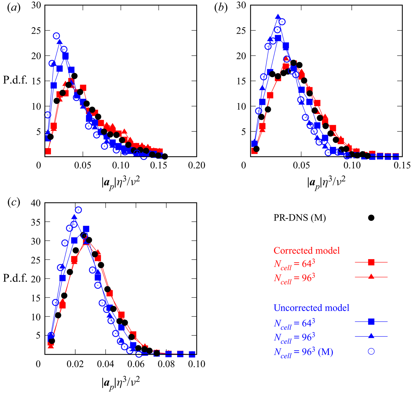
Figure 22. P.d.f.s of the magnitude of the particle acceleration: (a)  $t\epsilon _{0}/k_{f0}=0.54$, (b) $t\epsilon _{0}/k_{f0}=2.70$, (c) $t\epsilon _{0}/k_{f0}=4.87$. The results obtained by Mehrabadi et al. (Reference Mehrabadi, Horwitz, Subramaniam and Mani2018) are indicated by the notation (M). The vertical axis is scaled according to the figure in Mehrabadi et al. (Reference Mehrabadi, Horwitz, Subramaniam and Mani2018).
A.2. Effect of grid resolution
Figure 23 compares the result for the model coefficients (corresponding to figures 16 and 17) between the case I384D1 and the similar case with higher grid resolution  $N_{cell}=512^{3}$ (case I512D1). Note that the condition I384 corresponds to the lowest resolution case in the sense of $\eta /\varDelta$ (see table 1), and the D1 particle is more sensitive to the small flow structures than the D2 and D3 particles, which requires higher resolution for the D1 particle. In figures 23(b), 23(c) and 23(d), the effect of the grid resolution is smaller than the effect of $k_0R$. In figures 23(a), 23(e) and 23( f), the increasing trends of $C_{dev}^{pS}$, $C_{dev}^{f}$ and $C_{iso}^{f}$ with increasing $k_0R$ are observed similarly for both grid resolution cases, and the trends indicated in § 5.5 are unchanged. Therefore, the grid resolution in the present study is reasonable to estimate the behaviour of the particle stress models.

Figure 23. Model coefficients of the particle stress models for different grid resolutions. Open symbols represent case I384D1 ( $N_{cell}=384^{3}$), and filled symbols represent case I512D1 ( $N_{cell}=512^{3}$). Panels (a,c,e) are for the deviatoric part of the particle stress, while panels (b,d, f) are for the isotropic part. The sizes of the averaging volume are indicated by different line types.
Appendix B. External force on the staggered grid
To satisfy the continuity of the external force in the sense of the second-order central difference,  $\boldsymbol {a}_{\boldsymbol {k}}$ in (3.11) is determined further by another complex vector $\boldsymbol {b}_{\boldsymbol {k}}$ as
 \begin{equation} \boldsymbol{a}_{\boldsymbol{k}}=\boldsymbol{b}_{\boldsymbol{k}}- \frac{\boldsymbol{k}_\varDelta\boldsymbol{\cdot}\boldsymbol{b}_{\boldsymbol{k}}}{| \boldsymbol{k}_\varDelta|^{2}}\,\boldsymbol{k}, \end{equation}
where
 \begin{align} \boldsymbol{k}_\varDelta=\left( 1-\exp\left(-\frac{2{\rm \pi}\,\Delta x}{L_{cube}}\,\frac{k_x}{k_0}\right), 1-\exp\left(-\frac{2{\rm \pi}\,\Delta x}{L_{cube}}\,\frac{k_y}{k_0}\right), 1-\exp\left(-\frac{2{\rm \pi}\,\Delta x}{L_{cube}}\,\frac{k_z}{k_0}\right) \right), \end{align}
as explained below. The complex vector  $\boldsymbol {b}_{\boldsymbol {k}}$ satisfies the relations
 $$\begin{gather} \boldsymbol{b}_{\boldsymbol{k}}=\boldsymbol{b}^{*}_{-\boldsymbol{k}}, \end{gather}$$
 $$\begin{gather}\overline{\boldsymbol{b}_{\boldsymbol{k}}}=0, \end{gather}$$
 $$\begin{gather}\overline{\boldsymbol{b}_{\boldsymbol{k}}(t)\,\boldsymbol{b}_{\boldsymbol{k}}^{*}(t+s)}= 2\sigma^{2}\exp\left(-\frac{s}{T_L}\right){\boldsymbol{\mathsf{I}}}, \end{gather}$$
where the superscript  $*$ and the overline indicate the complex conjugate and the time average, respectively, and $T_L$ is the time scale.
Equation (B2) is different from that used in the original work (Eswaran & Pope Reference Eswaran and Pope1988) because of the difference in the discretisation method. Here, following the discussion on the fourth-order central difference scheme with the staggered arrangement of the variables by Takiguchi (Reference Takiguchi2000), the derivation of (B2) is summarised briefly for the second-order scheme adopted in the present study. Even though the discretisation scheme is different, the approach proposed by Takiguchi (Reference Takiguchi2000) is applicable for other schemes.
As the spectral method is used in Eswaran & Pope (Reference Eswaran and Pope1988), the complex vector  $\boldsymbol {a}_{\boldsymbol {k}}$ for the external force (3.10) should satisfy the continuity condition
 \begin{equation} \boldsymbol{k}\boldsymbol{\cdot}\boldsymbol{a}_{\boldsymbol{k}}=0, \end{equation}
and  $\boldsymbol {k}_{\varDelta }=\boldsymbol {k}$ is used instead of (B2). However, for the second-order central difference scheme with the staggered grid, the continuity condition takes the form
 \begin{equation} \frac{g_x^{i,j,k}-g_x^{i-1,j,k}}{\Delta x}+ \frac{g_y^{i,j,k}-g_y^{i,j-1,k}}{\Delta x}+ \frac{g_z^{i,j,k}-g_z^{i,j,k-1}}{\Delta x}=0, \end{equation}
where  $g_x$, $g_y$ and $g_z$ are components of $\alpha _c\boldsymbol {g}_{c}$ (see (3.10)) located at the definition points of the velocity components. The superscript indicates the index of the numerical grid point. According to (3.10),
 $$\begin{gather} g_x^{i,j,k}-g_x^{i-1,j,k}=\sum_{0<|\boldsymbol{k}|\leqslant\sqrt{2}k_0}a_{\boldsymbol{k}x} \exp(\sqrt{-1}\,\boldsymbol{k}\boldsymbol{\cdot}\boldsymbol{x}) \{ 1-\exp (-\sqrt{-1}\,k_x\,\Delta x)\} \end{gather}$$
 $$\begin{gather}g_y^{i,j,k}-g_y^{i,j-1,k}=\sum_{0<|\boldsymbol{k}|\leqslant\sqrt{2}k_0}a_{\boldsymbol{k}y} \exp(\sqrt{-1}\,\boldsymbol{k}\boldsymbol{\cdot}\boldsymbol{x}) \{ 1- \exp(-\sqrt{-1}\,k_y\,\Delta x)\} \end{gather}$$
 $$\begin{gather}g_z^{i,j,k}-g_z^{i,j,k-1}=\sum_{0<|\boldsymbol{k}|\leqslant\sqrt{2}k_0}a_{\boldsymbol{k}z} \exp(\sqrt{-1}\,\boldsymbol{k}\boldsymbol{\cdot}\boldsymbol{x}) \{ 1- \exp(-\sqrt{-1}\,k_z\,\Delta x)\} \end{gather}$$
are confirmed, where the imaginary unit is described by  $\sqrt {-1}$ instead of ${\rm i}$ to avoid ambiguity. Based on (B8)–(B10), the continuity is achieved by (B2).


 Open access