


1. Introduction
The study of oscillatory flow in porous media has applications in acoustics, seismology, coastal engineering and marine sciences, and possibly in the engineering of thermal and chemical processes. When a pressure wave with a wavelength significantly larger than the pore scale propagates through a porous medium, the pore fluid can be considered to be driven by an oscillatory pressure gradient (Johnson, Koplik & Dashen Reference Johnson, Koplik and Dashen1987). The propagation of sound through porous materials as well as of seismic waves through the Earth's crust can be described using the theory of Biot (Reference Biot1956a,Reference Biotb Reference Biot1962). The coefficients of this theory can be determined from the solution of the flow problem on the pore scale (Burridge & Keller Reference Burridge and Keller1981). In coastal engineering, oscillatory porous media flow is of interest in describing the interaction of water waves with rubble-mound breakwaters. To this end, several experimental investigations of oscillatory flow through sphere packs and rock samples have been undertaken by van Gent (Reference van Gent1993) and Hall, Smith & Turcke (Reference Hall, Smith and Turcke1995). Further applications of oscillatory porous media flow in the context of marine sciences include the water wave interaction with porous seabeds (Gu & Wang Reference Gu and Wang1991) or modelling flow in coral communities (Lowe et al. Reference Lowe, Shavit, Falter, Koseff and Monismith2008). For technical applications, oscillatory porous media flow can be of interest due to the increased heat transfer (Jin & Leong Reference Jin and Leong2006) or dispersion (Crittenden et al. Reference Crittenden, Lau, Brinkmann and Field2005) when compared to steady flow. Graham & Higdon (Reference Graham and Higdon2002) performed a broad investigation of oscillatory flow through two-dimensional porous media. They explored the effect of various types of oscillatory forcing, and demonstrated that a mean flow can be induced opposed to the mean pressure gradient. Moreover, they suggested that oscillatory flow could be applied as a filter to separate fluids of different viscosities. Thereby, an appropriately designed temporal waveform of the pressure gradient induces a mean flow in each fluid that points in opposite directions. Finally, the study of oscillatory flow is also a good starting point for the understanding and modelling of general unsteady flow.
Porous media are characterised by the presence of a macroscale  $L$ that is of the order of magnitude of the extent of the porous medium, and a microscale $l$ that is of the order of magnitude of the pore size. When $l \ll L$, the flow through porous media is described commonly in terms of aggregated quantities on the macroscale, for example, the filter velocity that represents the volume flow rate per cross-sectional unit area of the porous medium, and pressure differences over distances of the order ${O}(L)$. In the simplest case, Darcy's law relates these macroscopic quantities by the permeability $K$; however, it is applicable only to steady linear flow. For more general configurations, methods have been proposed to derive governing equations for the macroscale flow from first principles, i.e. the conservation laws for mass and momentum. Examples are the volume-averaging approach (Whitaker Reference Whitaker1986) or the homogenisation method (Ene & Sanchez-Palencia Reference Ene and Sanchez-Palencia1975; Bensoussan, Lions & Papanicolaou Reference Bensoussan, Lions and Papanicolaou1978; Lévy Reference Lévy1987; Hornung et al. Reference Hornung, Kadanoff, Marsden, Sirovich, Wiggins and John1997). In the volume-averaging approach, the differential equations are averaged locally over a so-called representative elementary volume of the porous medium. Different weighting functions can be used in the definition of the volume average, e.g. a top-hat or Gaussian kernel. The resulting volume-averaged Navier–Stokes equations are unclosed, as they contain microscale quantities describing the flow resistance and dispersion in the pore space. Formally, the equations can be closed by solving a boundary value problem on the representative elementary volume (Whitaker Reference Whitaker1986 Reference Whitaker1996; Lasseux, Valdés-Parada & Bellet Reference Lasseux, Valdés-Parada and Bellet2019). For periodic porous media, the theory of homogenisation presents an alternative to the volume-averaging approach. An artificial spatial coordinate $\boldsymbol {y}=(L/l) \boldsymbol {x}$ is introduced in addition to the spatial coordinate $\boldsymbol {x}$. Using a perturbation series approach with the small variable $l/L$, the flow problem can be separated into a $\boldsymbol {y}$-dependent boundary problem on the unit cell for which the $\boldsymbol {x}$-dependent terms act as source terms, and a macroscale problem dependent on $\boldsymbol {x}$ and $\boldsymbol {y}$. In conclusion, both the volume-averaging and the homogenisation approach lead to the question of how the flow on a representative elementary volume or unit cell of the porous medium and its integral properties are related to the macroscopic pressure gradient. In the present work, we investigate this dependency for laminar oscillatory flow in the linear and weakly nonlinear regime.
In the following, we review models that have been used to relate the macroscopic velocity to the macroscopic pressure gradient. The macroscale quantities are expressed in terms of the superficial volume average
 \begin{equation} \left\langle\psi\right\rangle_{\mathrm{s}} = \frac{1}{V} \int_{V_{{f}}} \psi \,\mathrm{d}V, \end{equation}
and the intrinsic volume average
 \begin{equation} \left\langle\psi\right\rangle_{\mathrm{i}} = \frac{1}{V_{{f}}} \int_{V_{{f}}} \psi \,\mathrm{d}V, \end{equation}
where  $V_{{f}}$ is the fluid volume, and $V$ is the combined fluid and solid volume of the unit cell. The averages are linked by the porosity $\epsilon = V_{{f}}/V$ as $\left \langle \psi \right \rangle _{\mathrm {s}}=\epsilon \left \langle \psi \right \rangle _{\mathrm {i}}$.
For steady flow, a widely accepted description of the resistance behaviour is given through the Forchheimer equation (Forchheimer Reference Forchheimer1901)
 \begin{equation} f_x = a \left\langle u\right\rangle_{\mathrm{s}} + b \left\langle u\right\rangle_{\mathrm{s}}^2, \end{equation}
where  $f_x$ represents the macroscopic pressure gradient $-\boldsymbol {\nabla }\!\left \langle p \right \rangle _{\mathrm {i}}$, and $\left \langle u \right \rangle _{\mathrm {s}}$ is the superficial velocity. The coefficients $a$ and $b$ are usually determined experimentally. Ergun (Reference Ergun1952) proposed porosity-dependent correlations for these coefficients, resulting in the Ergun equation, which have been confirmed in later studies (Macdonald et al. Reference Macdonald, El-Sayed, Mow and Dullien1979). Whitaker (Reference Whitaker1996) presented a theoretical derivation of the Forchheimer equation from the volume-averaged Navier–Stokes equations. A comprehensive review of the resistance behaviour in stationary porous media flow was given by Wood, He & Apte (Reference Wood, He and Apte2020). One can assume that in oscillatory flow at very low frequencies, there exists a quasi-steady regime in which the resistance behaviour can be described appropriately by the Forchheimer equation and its steady-state coefficients.
Oscillatory flow at small amplitudes is well understood theoretically and can be described accurately by the so-called equivalent fluid model based on the work of Johnson et al. (Reference Johnson, Koplik and Dashen1987) and Champoux & Allard (Reference Champoux and Allard1991). A comprehensive review of the theory was given by Lafarge (Reference Lafarge2009). Chapman & Higdon (Reference Chapman and Higdon1992) verified the model of Johnson et al. (Reference Johnson, Koplik and Dashen1987) with highly accurate numerical solutions of the unsteady Stokes equations for oscillatory flow through sphere packs. Turo & Umnova (Reference Turo and Umnova2013) proposed a model similar to the model of Johnson et al. (Reference Johnson, Koplik and Dashen1987) that is formulated in the time domain and features a Forchheimer-type nonlinearity. They compared their model to data from a shock tube experiment, and obtained ‘satisfactory agreement’.
Sollitt & Cross (Reference Sollitt and Cross1972) extended the Forchheimer equation (1.3) with an acceleration term to describe unsteady nonlinear flow in porous media. The unsteady Forchheimer equation possesses a sensible low-frequency limit – the steady Forchheimer equation – but it does not comply with the theoretical high-frequency limit derived by Johnson et al. (Reference Johnson, Koplik and Dashen1987). Furthermore, there does not seem to be a general agreement in the literature on the choice of coefficients; based on an extensive experimental investigation of oscillatory porous media flow, van Gent (Reference van Gent1993) suggested correlations for the coefficients in the unsteady Forchheimer equation. Notably, both the coefficient of the acceleration term and of the nonlinear term depend on the frequency of oscillation. Burcharth & Andersen (Reference Burcharth and Andersen1995) noted that the coefficients of the unsteady Forchheimer equations are in principle time-dependent. This can be seen in the study of Hall et al. (Reference Hall, Smith and Turcke1995), who applied a least squares fit to determine average values for the coefficients of the linear and nonlinear terms, and obtained a temporally varying and sometimes even negative acceleration coefficient. For strongly accelerated flow, a further arguable point is that the nonlinearity in the unsteady Forchheimer equation depends only on the instantaneous superficial velocity  $\left \langle u \right \rangle _{\mathrm {s}}$. To the best of our knowledge, this assumption has yet to be examined. Hence, in the absence of a generally valid model, it would be interesting to know under which circumstances oscillatory flow can be considered as linear and thus be described reliably by the equivalent fluid model, and when by contrast we have to resort to nonlinear models.
In this work, we consider laminar oscillatory flow through a periodic sphere pack. First, we seek to address the question of for which values of amplitude and frequency of the oscillatory forcing (represented by the Hagen number  $ {\textit {Hg}}$ and the Womersley number $ {\textit {Wo}}$) nonlinear effects have to be considered. We establish a boundary between linear and nonlinear flow in the $ {\textit {Hg}}$– $ {\textit {Wo}}^2$ parameter space based on the scaling of the volume-averaged velocity and kinetic energy with the Hagen number, and we use the magnitude of the Fourier series coefficients of the velocity field to assess the importance of nonlinear effects.
Second, we investigate how the nonlinearity affects the instantaneous velocity fields at maximum superficial velocity. We find that a key effect is the loss of fore–aft symmetry of the flow. We look into the temporal evolution of this loss of symmetry in order to determine when nonlinear effects occur during the cycle. We observe a phase shift between the superficial velocity and the nonlinear effects at higher frequencies that raises doubts as to whether the modelling of the nonlinearity with a Forchheimer-type closure is appropriate in unsteady flow.
Third, we provide a consistent description of the flow in the frequency domain. We explain the emergence of a time-averaged velocity field, and we discuss the interaction among the Fourier modes that results in a variation of the strength of nonlinear effects throughout the cycle.
2. Problem statement
2.1. Geometry of the sphere pack
We consider a hexagonal close-packed arrangement of spheres as a porous medium. The centre coordinates of the spheres  $(i,j,k)$ in hexagonal close-packed arrangement are
 \begin{equation} \begin{bmatrix} x_c \\ y_c \\ z_c \end{bmatrix} = \begin{bmatrix} 2 i + (j +k) \bmod 2\\ \sqrt{3}\left[j + \frac{1}{3}(k \bmod 2)\right]\\ \frac{2\sqrt{6}}{3}\,k \end{bmatrix}\frac{d}{2}, \end{equation}
and the sphere pack has the periodicities  $d$,
$d$,  $\sqrt {3}\,d$ and $\frac {2\sqrt {6}}{3}\,d$ in the $x$-,
$x$-,  $y$- and $z$-directions, respectively. The hexagonal sphere pack has a $60^\circ$ rotational symmetry in the $x$–
$x$– $y$ plane, and a reflection symmetry in the $z$-direction. The porosity of the sphere pack is
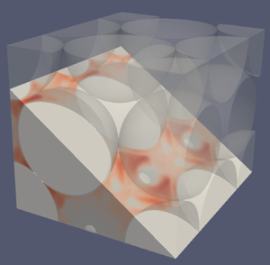
  $\epsilon = 1-\frac{\rm \pi}{3\sqrt{2}}=0.26$. Figure 1(a) shows the part of the sphere pack that is contained in the simulation domain. A peculiarity of the hexagonal sphere pack geometry is that there exist straight channels along the $x$-direction with contact points in the centres of the channels. This can be seen in figure 1(b), which shows a section through the sphere pack along the plane $\frac {\sqrt {3}}{3} y -\frac {\sqrt {6}}{3}z=0$. This plane is parallel to the cut plane used in the analysis of Sakai & Manhart (Reference Sakai and Manhart2020) and results in shifted, but otherwise equivalent, flow fields.

Figure 1. (a) Hexagonal sphere pack in the simulation domain. (b) Section through the hexagonal sphere pack along the plane  $\frac {\sqrt {3}}{3}y -\frac {\sqrt {6}}{3}z=0$. The contact points are marked by red dots. The area highlighted in blue is the region for which velocity fields are shown in figures 10–15.
2.2. Governing equations
The flow in the pore space is governed by the incompressible Navier–Stokes equations
 $$\begin{gather} \boldsymbol{\nabla}\boldsymbol{\cdot}\boldsymbol{u} =0, \end{gather}$$
 $$\begin{gather}\frac{\partial \boldsymbol{u}}{\partial t} + \boldsymbol{\nabla} \boldsymbol{\cdot} \left(\boldsymbol{u}\otimes \boldsymbol{u}\right) ={-}\frac{1}{\rho}\,\boldsymbol{\nabla} p + \nu\,\Delta\boldsymbol{u} + \frac{1}{\rho}\,\boldsymbol{f}, \quad\text{with }\ \boldsymbol{f}=f_x\sin(\varOmega t)\,\boldsymbol{e}_x, \end{gather}$$
satisfies no-slip and triple periodic boundary conditions, and is at rest at  $t=0$:
 $$\begin{align} \boldsymbol{u}(\boldsymbol{x},t) &= 0 \quad\quad\quad\quad\quad \text{for }\boldsymbol{x}\text{ on the surface of the spheres}, \end{align}$$
 $$\begin{align}\boldsymbol{u}(\boldsymbol{x},t) &= \boldsymbol{u}(\boldsymbol{x}+\boldsymbol{L},t) \quad \text{for }\boldsymbol{L} \in \left\lbrace L_x\,\boldsymbol{e}_x, L_y\,\boldsymbol{e}_y, L_z\,\boldsymbol{e}_z \right\rbrace, \end{align}$$
 $$\begin{align}p(\boldsymbol{x},t) &= p(\boldsymbol{x}+\boldsymbol{L},t) \quad \text{for }\boldsymbol{L} \in \left\lbrace L_x\,\boldsymbol{e}_x,L_y\,\boldsymbol{e}_y,L_z\,\boldsymbol{e}_z \right\rbrace, \end{align}$$
 $$\begin{align}\boldsymbol{u}(\boldsymbol{x},0) &= 0. \end{align}$$
The periods  $L_x$, $L_y$ and $L_z$ denote the size of the simulation domain in the $x$-,
$x$-,  $y$- and $z$-directions, respectively.
The sinusoidally oscillating force  $\boldsymbol {f}$ is constant in space and represents a macroscopic pressure gradient. In inviscid flow, this configuration would lead to a potential flow proportional to $1-\cos (\varOmega t)$ and therefore an oscillation with non-zero mean; however, in viscous flow, the influence of the initial condition decays with time, and the flow reaches a steady oscillation with zero mean. We did not investigate a cosinusoidal forcing, as the starting flow would resemble closely the flow of a fluid at rest subject to a constant force, which was studied by Sakai & Manhart (Reference Sakai and Manhart2020), and the flow after the decay of the transient would be the same as with the sinusoidal force (albeit shifted in time).
2.3. Dimensional analysis
In this subsection, we derive and discuss the independent parameters that determine the flow uniquely. The problem as stated in §§ 2.1 and 2.2 is to determine the velocity field  $\boldsymbol {u}$ as a function of the position $\boldsymbol {x}$, the time $t$, the fluid density $\rho$, the kinematic viscosity $\nu$, and the amplitude and frequency of the forcing $f_x$ and $\varOmega$. We deliberately do not consider the porosity $\epsilon$ and the permeability $K$ in the dimensional analysis as they depend solely on the geometry and the sphere diameter $d$. A systematic study of the effects of the pore geometry is beyond the scope of our present work because adding additional parameters would increase significantly the cost of this study.
We now perform a dimensional analysis (Buckingham Reference Buckingham1914). Choosing the density  $\rho$, the kinematic viscosity $\nu$ and the sphere diameter $d$ as reference variables, we obtain the dimensionless ratios
 \begin{equation} \varPi_1 = \frac{\boldsymbol{x}}{d},\quad \varPi_2 = \frac{\nu t}{d^2},\quad \varPi_3 = \frac{f_xd^3}{\rho\nu^2} \quad\text{and}\quad \varPi_4 = \frac{\varOmega d^2}{\nu}. \end{equation}
We can identify  $\varPi _3$ as the Hagen number $ {\textit {Hg}} =f_xd^3/(\rho \nu ^2)$ (Martin Reference Martin2010; Awad Reference Awad2013), which represents a dimensionless pressure gradient in viscous units, and $\sqrt {\varPi _4}$ as the Womersley number $ {\textit {Wo}} =\sqrt {\varOmega d^2/\nu }$ (Womersley Reference Womersley1955), which represents the ratio of the sphere diameter $d$ to the thickness of Stokes’ oscillatory boundary layer. Alternatively, $ {\textit {Wo}}^2$ can be interpreted (up to a constant) as the ratio of the viscous time scale $d^2/\nu$ to the period of excitation $T=2{\rm \pi} /\varOmega$.
From the  $\varPi$ theorem (Buckingham Reference Buckingham1914), we infer that the velocity field can be represented as a function
 \begin{equation} \frac{\boldsymbol{u}d}{\nu}=\boldsymbol{\varPhi}\left(\frac{\boldsymbol{x}}{d}, \frac{\nu t}{d^2}; {\textit{Hg}}, {\textit{Wo}}\right), \end{equation}
with  $ {\textit {Hg}}$ and $ {\textit {Wo}}$ as two independent parameters. A dimensionless form of the Navier–Stokes equations follows as
 \begin{equation} \frac{\partial \hat{\boldsymbol{u}}}{\partial \hat{t}} + \hat{\boldsymbol{\nabla}} \boldsymbol{\cdot} \left(\hat{\boldsymbol{u}}\otimes \hat{\boldsymbol{u}}\right) ={-}\hat{\boldsymbol{\nabla}} \hat{p} + \hat{\Delta}\hat{\boldsymbol{u}} + {\textit{Hg}}\sin({\textit{Wo}}^2 \hat{t})\,\boldsymbol{e}_x, \end{equation}
where  $\hat {\boldsymbol {u}}=\boldsymbol {u} d/\nu$, $\hat {\boldsymbol {x}}=\boldsymbol {x}/d$, $\hat {t}=\nu t/d^2$ and $\hat {p}= pd^2/(\rho \nu ^2)$. While this is not the only possible way to non-dimensionalise the equations, the present form illustrates the meanings of the Hagen and Womersley numbers. Generally, different dimensionless forms are appropriate for different flow regimes.
A Reynolds number can be obtained by taking a suitable point value or average of the dimensionless velocity field (2.5). Here, we define the Reynolds number based on the sphere diameter and the maximum superficial volume-averaged velocity after the transient has decayed:
 \begin{equation} {\textit{Re}} = \limsup_{t\to\infty} \frac{\left\langle\boldsymbol{u}\right\rangle_{\mathrm{s}} d}{\nu}. \end{equation}
Since the volume-averaging and the maximum suppress the spatial and temporal dependencies, the Reynolds number can then be expressed as a function of two independent parameters  $ {\textit {Wo}}$ and $ {\textit {Hg}}$. Note that this Reynolds number is related to the pore Reynolds number defined, for example, by Wood et al. (Reference Wood, He and Apte2020) via the porosity as $ {\textit {Re}} = \epsilon \, {\textit {Re}}_{p}$. The Hagen number has been employed occasionally in other works in the guise of a pressure-gradient-based Reynolds number (Ene & Sanchez-Palencia Reference Ene and Sanchez-Palencia1975; Firdaouss, Guermond & Le Quéré Reference Firdaouss, Guermond and Le Quéré1997; Iervolino, Manna & Vacca Reference Iervolino, Manna and Vacca2010; Lasseux et al. Reference Lasseux, Valdés-Parada and Bellet2019) or a dimensionless body force (Graham & Higdon Reference Graham and Higdon2002). As the Reynolds number expresses the ratio of the characteristic magnitude of the convective and viscous terms in the Navier–Stokes equations, whereas the dimensionless group $\varPi _3 = f_x d^3/(\rho \nu ^2)$ represents the ratio of the body force to the viscous term, we refrained from calling this a Reynolds number and used the definition of Martin (Reference Martin2010) and Awad (Reference Awad2013) instead.
3. Methodology
3.1. Description of numerical methods
We performed direct numerical simulation of the incompressible Navier–Stokes equations (2.2) with our in-house code MGLET (Manhart, Tremblay & Friedrich Reference Manhart, Tremblay and Friedrich2001; Manhart Reference Manhart2004; Peller et al. Reference Peller, Duc, Tremblay and Manhart2006; Peller Reference Peller2010; Sakai et al. Reference Sakai, Mendez, Strandenes, Ohlerich, Pasichnyk, Allalen and Manhart2019). For spatial discretisation, MGLET uses an energy-conserving central second-order finite volume method based on a Cartesian grid with a staggered arrangement of variables (Harlow & Welsh Reference Harlow and Welsh1965; Patankar Reference Patankar1980). For time integration, we employ an explicit three-stage third-order low-storage Runge–Kutta method (Williamson Reference Williamson1980). We employ a variant of the fractional-step method (Chorin Reference Chorin1968) in which in every substep of the Runge–Kutta scheme the stage velocities are made divergence-free by a pressure update. The pressure update is obtained by solving a Poisson equation that is constructed by applying the discrete divergence operator to the stage velocity and the gradient of the pressure update; see e.g. Ferziger & Perić (Reference Ferziger and Perić2002).
Complex geometries are treated using an embedded boundary approach (Peller et al. Reference Peller, Duc, Tremblay and Manhart2006). We now give a brief overview of the employed algorithm. The simulation geometry is determined as a piecewise planar description based on the intersection points of the Cartesian grid with the specified body geometry. The momentum equation is solved only on cells that lie completely within the fluid domain. The interface cells are used to enforce the no-slip boundary condition using a ghost-cell approach (Peller et al. Reference Peller, Duc, Tremblay and Manhart2006). The velocities in the interface cells are computed using two kinds of interpolation (Peller Reference Peller2010). To evaluate velocity gradients and the convected velocities, we set a second-order accurate point value computed by linear least squares interpolation (extrapolation). To compute the convecting velocities and the divergence, we set an approximation to the mass fluxes through the respective pressure cell face. An iterative flux correction procedure that is coupled to the pressure correction ensures conservation of mass for the interface cells (Peller Reference Peller2010). In this scheme, no boundary conditions are needed for the pressure at the embedded boundary.
3.2. Verification of the numerical method
In order to verify the convergence of our code with spatial grid refinement, we simulated steady flow in a simple cubic lattice of spheres at porosity  $\epsilon =0.875$ driven by a constant-volume force with $ {\textit {Hg}}=10^{-4}$. This configuration was investigated previously by Chapman & Higdon (Reference Chapman and Higdon1992), who obtained permeability $K=0.10355d^2$ by solving the Stokes equations with a solid harmonics collocation method. Since their method is based on a harmonic expansion that satisfies exactly the no-slip boundary condition on the spheres, we consider their method as very accurate and we use their results to verify our scheme.
We computed the flow around a sphere centred in a cubic domain of side length  $1.612d$ with periodic boundary conditions at grid resolutions $12.4$, $24.8$, $49.6$, $99.3$, $198.5$ and $397$ cells per sphere diameter (cpd). On the finest grid, we obtained permeability $K_{397} = 0.10358d^2$. For this value, we estimated the relative error with the grid convergence index (Roache Reference Roache1994; Celik et al. Reference Celik, Urmila, Roache, Freitas, Coleman and Raad2008), which resulted in a value $ {\textit {GCI}}_{fine}=2.8\times 10^{-5}$ at apparent order $p=1.8$. Our value differs from the result of Chapman & Higdon (Reference Chapman and Higdon1992) only in the last reported digit, when their value is renormalised to the sphere diameter instead of the domain length. At $24.8$ cpd, the computed permeability error is well below $1\,\%$. Furthermore, we evaluated the superficial average of the kinetic energy $\left \langle k \right \rangle _{\mathrm {s}}=\left \langle \frac {1}{2}\rho \boldsymbol {u}^2\right \rangle _{\mathrm {s}}$ and the $u$-velocity at the point $\boldsymbol {P}=(0.8 d, 0.8 d, 0.8 d)$ relative to the centre of the sphere. These values are plotted as a function of the grid spacing in figure 2. It can be seen that the relative error decreases at approximately second order with the grid spacing $\Delta x$ over three orders of magnitude.

Figure 2. Grid convergence for steady Stokes flow in a simple cubic lattice of spheres at porosity  $\epsilon =0.875$. The permeability $K$, the velocity at the probe point $\boldsymbol {P}=(0.8 d, 0.8 d, 0.8 d)$ and the kinetic energy $\left \langle k \right \rangle _{\mathrm {s}}$ of the flow field are compared to their respective values at the finest grid resolution $d/\Delta x=397$.
Thus we have demonstrated that for the given test case, the embedded boundary method achieves the theoretical second-order convergence and converges to a result close to the reference value.
3.3. Simulation set-up
The objective of this study is to investigate the boundary between the linear and nonlinear regimes in the  $ {\textit {Hg}}$– $ {\textit {Wo}}$ parameter space for oscillating flow in a hexagonal sphere pack. Therefore, we tried to cover unknown and computationally affordable regions in this parameter space beyond the linear regime, which for this particular geometry had already been investigated by Zhu & Manhart (Reference Zhu and Manhart2016).
In a first step, we could assume that nonlinear effects appear if the maximum Reynolds number within a cycle exceeds a certain threshold. Based on the results of Sakai & Manhart (Reference Sakai and Manhart2020), who observed linear behaviour for  $ {\textit {Re}} \leqslant 1$ in steady flow through a hexagonal sphere pack, we chose a threshold value $ {\textit {Re}}=1$. For linear flow, two asymptotes exist for the maximum velocity in a cycle as a function of the Womersley number. At the low-frequency limit, the oscillation amplitude reaches the values of the steady state – this is the quasi-steady regime. Here, the end of the linear regime could be estimated at $ {\textit {Hg}}={d^2}/{K} \approx 5776$ using Darcy's law (which reads $ {\textit {Re}}=({K}/{d^2})\, {\textit {Hg}}$ in non-dimensional form) and permeability value $K=1.731\times 10^{-4}\,d^2$ (Sakai & Manhart Reference Sakai and Manhart2020). In the high-frequency limit, the amplitude decays with $ {\textit {Wo}}^{-2}$ for constant $ {\textit {Hg}}$. The transition between the low- and high-frequency regimes occurs close to Womersley number $ {\textit {Wo}}_0 = \sqrt {{\epsilon d^2}/({\alpha _{\infty }K})}=30.5$; this value marks the intersection of the low- and high-frequency asymptotes of linear flow (Pride, Morgan & Gangi Reference Pride, Morgan and Gangi1993). To cover the range departing from the quasi-steady behaviour, we therefore performed simulations at three different Womersley numbers, $ {\textit {Wo}}=10$, $31.62$ and $100$. The simulation parameters were chosen to lie on a logarithmic grid, leading to equispaced points in the log-log plot and thus a uniform point density over the orders of magnitudes. For each of the three Womersley numbers, we selected various Hagen numbers lying above the linear limit in the quasi-steady regime $ {\textit {Hg}}\approx 5776$. Figure 3(a) shows the simulations in the $ {\textit {Hg}}$– $ {\textit {Wo}}^2$ parameter space.

Figure 3. Study design. (a) Simulations at low (LF), medium (MF) and high frequency (HF) in the  $ {\textit {Hg}}$– $ {\textit {Wo}}^2$ parameter space. The dotted line indicates the condition $ {\textit {Re}}=1$ in quasi-steady Darcy flow. The dashed line indicates the Womersley number $ {\textit {Wo}}_0$ that represents the intersection of the low- and high-frequency asymptotes in the linear regime. The arrows indicate the changes in the dimensionless numbers if the respective parameters are doubled. (b) Top view of the sphere pack cut in the symmetry plane $z=\frac {\sqrt {6}}{3}\,d$. The red frame represents the simulation domain that consists of two unit cells (indicated by the dashed red line). The coloured areas and arrows represent shift invariances of the geometry in the $x$-direction and at a $60^\circ$ angle to the $x$-direction. Consequently, the simulation domain contains eight repetitions of the minimum box represented by the coloured areas.
We chose a domain size  $L_x=2d$, $L_y=\sqrt {3}\,d$ and $L_z=\frac {2\sqrt {6}}{3}\,d$ with periodic boundary conditions for $\boldsymbol {u}$ and $p$ in the $x$-,
$x$-,  $y$- and $z$-directions. This domain represents one unit cell in the $y$- and $z$-directions, but includes two periodic repetitions of the unit cell in the $x$-direction. In the following, we motivate this particular choice for the size of the simulation domain. On the one hand, linear flow has the same symmetries and periodicity as the sphere pack and it can be fully represented with a domain consisting of one unit cell. On the other hand, nonlinear flow does not have to adhere to the symmetries of the sphere pack and also admits solutions that are not periodic on the unit cell. Then the periodic boundary conditions prevent the formation of structures larger than the simulation domain. The selected simulation domain contains two spheres in every lattice direction and possesses multiple symmetries: the sphere pack has a reflection symmetry about the midplane in the $z$-direction, and two shift invariances in the $x$-direction and at a $60^\circ$ angle to the $x$-direction (see figure 3b). For all simulations presented in this work, we have verified numerically that the velocity field satisfies these symmetries. We expect that the above symmetries of the flow in directly adjacent pores would have to be broken before a breaking of the periodicity in the $y$- and $z$-direction – symmetries between second-order neighbours – could be observed. Therefore, we limit the domain size to one period in the $y$- and $z$-directions. The relatively compact simulation domain allows us to employ high grid resolutions in order to obtain accurate solutions.
For all cases, we employed a uniform Cartesian grid of nearly cubical cells with aspect ratio 1.00 : 0.99 : 0.98 due to the incommensurate periodicities of the domain. The simulations were performed at grid resolutions 48, 96, 192 and 384 cpd. For the simulation HF4, an additional simulation was performed at grid resolution 768 cpd. These resolutions were chosen based on the convergence of the volume-averaged velocity  $\left \langle \boldsymbol {u}\right \rangle _{\mathrm {s}}$ and the volume-averaged kinetic energy $\left \langle k \right \rangle _{\mathrm {s}}$ (see § 3.4). For comparison, Sakai & Manhart (Reference Sakai and Manhart2020) used grid resolution 320 cpd to simulate transient nonlinear and turbulent flow in a hexagonal sphere pack using the same code, and He et al. (Reference He, Apte, Finn and Wood2019) used resolution 250 cpd to simulate turbulent flow at $ {\textit {Re}}= 750$ in a face-centred cubic sphere pack of the same porosity.
The time step was chosen to meet the stability limits for the explicit Runge–Kutta scheme; the Courant–Friedrich–Lewy number was always below  $0.33$, and the diffusion number was always below $0.35$. This resulted in at least 40 000 time steps per cycle of oscillation. We applied a uniform body force $\boldsymbol {f} = f_x \sin (\varOmega t)\,\boldsymbol {e}_x$ in the $x$-direction to drive the flow. As the flow starts from rest, this forcing causes a transient oscillation. The transient establishes a net superficial velocity within a cycle, and leads to differences in the peak values of $\left \langle \boldsymbol {u}\right \rangle _{\mathrm {s}}$ and $\left \langle k \right \rangle _{\mathrm {s}}$ within one cycle as well as from one cycle to the next. We ran our simulations until these differences were below $1\,\%$ of the peak values. Thus the transient has decayed sufficiently to show a periodic solution in time.
For post-processing the simulations, we collected the following data: time-resolved data were obtained for volume-averaged quantities  $\left \langle \boldsymbol {u}\right \rangle _{\mathrm {s}}$, $\langle u^2\rangle _{\rm s}$, $\langle v^2\rangle _{\rm s}$ and $\langle w^2\rangle _{\rm s}$. Complete three-dimensional fields of $\boldsymbol {u}$ and $p$ have been collected at a sampling rate between 25 and 100 snapshots per cycle, depending on the simulation.
3.4. Grid convergence
In this subsection, we discuss the dependency of our simulation results on the grid resolution. We choose two quantities for assessing the quality of the simulations: first, the Reynolds number  $ {\textit {Re}}$ based on the maximum of $\left \langle u \right \rangle _{\mathrm {s}}$ in steady oscillatory flow as defined in (2.7); and second, the space–time $L^2$-norm of the velocity field over the last period of each simulation, as
 \begin{equation} \left\Vert \boldsymbol{u}\right\Vert_{L^2}^2 = \int_{V_{f}} \int_{T} |\boldsymbol{u}|^2\,\mathrm{d}t \,\mathrm{d}V . \end{equation}
 This quantity can be interpreted as the signal energy of the velocity field. It was calculated as the sum of the quantities  $\langle u^2\rangle _{\rm s}$, $\langle v^2\rangle _{\rm s}$ and $\langle w^2\rangle _{\rm s}$, which were collected in every time step. Therefore, the square of every velocity value in every time step of the last period contributes to $\Vert \boldsymbol {u}\Vert _{L^2}^2$. Due to reasons explained below, we observe non-monotonic convergence of these quantities. Thus the grid convergence index (Roache Reference Roache1994) does not give meaningful results, and we report explicitly the errors observed at the various grid resolutions.
Table 1 contains the relative differences of  $\Vert \boldsymbol {u}\Vert _{L^2}^2$ with respect to their solutions at 384 cpd and the Reynolds number $ {\textit {Re}}$ within the last cycle for the different resolutions. Generally, the errors increase with Womersley and Hagen numbers. For a Womersley number of $10$, an error in $\Vert \boldsymbol {u}\Vert _{L^2}^2$ below $0.2\,\%$ has been achieved with 192 cpd, and at $ {\textit {Wo}}=31.62$, the maximum error is below $1.65\,\%$. At $ {\textit {Wo}}=100$, the differences between 192 and 384 cpd remain larger. The maximum error is $-4.60\,\%$ for simulation HF4 at $Wo =100$ and $ {\textit {Hg}}=10^{7.25}$. To assess the error of the simulation at 384 cpd for this case, we performed an additional grid refinement to 768 cpd. The error at the resolution 384 cpd with respect to the more finely resolved simulation is $0.17\,\%$.
Table 1. Grid convergence of the velocity field  $\boldsymbol {u}(\boldsymbol {x},t)$ in steady oscillation. The relative error in $\Vert \boldsymbol {u}\Vert _{L^2}^2$ is defined as $e_{res} = ( \Vert \boldsymbol {u}_{res}\Vert _{L^2}^2-\Vert \boldsymbol {u}_{384}\Vert _{L^2}^2 ) / \Vert \boldsymbol {u}_{384}\Vert _{L^2}^2$, and as $e_{res} = ( \Vert \boldsymbol {u}_{res}\Vert _{L^2}^2-\Vert \boldsymbol {u}_{768}\Vert _{L^2}^2 ) / \Vert \boldsymbol {u}_{768}\Vert _{L^2}^2$ for HF4. The Reynolds number $ {\textit {Re}}$ is defined according to (2.7).

The Reynolds number computed according to (2.7) ranges from values below  $1.0$ to values around $73$ at the lower Womersley numbers, and $ {\textit {Re}}=251.8$ at $ {\textit {Wo}}=100$. From table 1, we see that the simulations have relative errors in $ {\textit {Re}}$ below $0.5\,\%$ at $Wo =10$, below $0.2\,\%$ at $Wo =31.62$, and below $0.7\,\%$ at $Wo =100$.
In contrast to the test case of § 3.2, we do not achieve the theoretical order of accuracy of our code. We explain this decrease of accuracy order by the presence of contact points between the spheres. These degrade the convergence of the pore volume represented in the Cartesian grid by the embedded boundary method. The representation of the spheres by a plane segment in each Cartesian cell intersecting the sphere surface leads to an overestimation of the pore volume, so the local pore volume decreases with grid refinement. The blocking of the thin gap between spheres in contact, however, leads to a local underestimation of the pore volume, so the pore volume around the contact points increases with grid refinement. These two effects taken together lead to a non-monotonic convergence of the porosity. At the finest grid resolution, 384 cpd, the relative error in the pore volume is  $-0.16\,\%$.
The influence of blocked pore space around the contact points increases with the Womersley number and could explain the increase in error with  $ {\textit {Wo}}$. At higher frequencies, the flow has a boundary structure (Schlichting & Gersten Reference Schlichting and Gersten2006). With increasing $ {\textit {Wo}}$, the boundary layer thickness along the surface of the spheres decreases, and the velocity field approaches the potential flow solution. Cox & Cooker (Reference Cox and Cooker2000) showed for the case of potential flow around a sphere touching an infinite plate that the velocity potential behaves as $r^{\sqrt {2}-1}$ close to the contact point, leading to a singularity in the velocity. As the boundary condition on the plate is identical to a symmetry boundary condition, we expect the same behaviour at the contact point of two spheres. Hence for increasing Womersley number, the velocity magnitude and gradients in the immediate vicinity of the contact points increase and become asymptotically singular. For high Womersley numbers, this behaviour leads to prohibitive resolution requirements.
In summary, all simulations possess a relative difference below  $1.2\,\%$ in the Reynolds number as well as in the $L^2$-norm of the velocity field between the second-finest and finest grids. However, due to the presence of contact points, we do not observe the theoretical order of accuracy of our code. We observed an increase in error with the Hagen and Womersley numbers that we explain by the reduction of the boundary layer thickness on the spheres and the consequently increasing importance of the area close to the contact points.
3.5. Validation for quasi-steady flow and for linear flow
In this subsection, we validate our simulation results against data from the literature for the steady and linear flow regimes. In the low-frequency limit ( $ {\textit {Wo}}\to 0$), the flow can be considered as a steady flow at every instant. The amplitude in steady flow can be described by the Ergun equation (Ergun Reference Ergun1952) made dimensionless with $\rho$, $d$ and $\nu$:
 \begin{equation} {\textit{Hg}} = A\,\frac{(1-\epsilon)^2}{\epsilon^3}\,{\textit{Re}} + B\,\frac{1-\epsilon}{\epsilon^3}\,{\textit{Re}}^2 . \end{equation}
Based on ample experimental data, the coefficients have the values  $A=180$ and $B=1.8$ for porous media consisting of smooth particles (Macdonald et al. Reference Macdonald, El-Sayed, Mow and Dullien1979). For the hexagonal sphere pack, Sakai & Manhart (Reference Sakai and Manhart2020) have given a similar correlation based on direct numerical simulation results. In figure 4(a), the Reynolds number based on the amplitude of the superficial velocity in our simulations is compared with the Reynolds number observed in steady flow at the same Hagen number. For small $ {\textit {Hg}}$, the amplitude is proportional to the Hagen number, as indicated by the horizontal asymptote. For larger $ {\textit {Hg}}$, the amplitude increases sublinearly with $ {\textit {Hg}}$ due to additional nonlinear drag. As expected, the simulations LF1–LF4 at $ {\textit {Wo}}=10$ ( $+$ symbols) show good agreement with the steady flow, whereas the amplitudes of the simulations at $ {\textit {Wo}}=31.62$ and $ {\textit {Wo}}=100$ are significantly smaller than in the steady flow.

Figure 4. Comparison of the amplitude of the superficial velocity in our simulations (black symbols) with  $ {\textit {Re}}$ observed in (a) steady and (b) linear flow. The values are normalised with the amplitude predicted by Darcy's law. (a) Blue line, Ergun equation (Macdonald et al. Reference Macdonald, El-Sayed, Mow and Dullien1979); red dashed line, Sakai & Manhart (Reference Sakai and Manhart2020). (b) Blue line, model of Pride et al. (Reference Pride, Morgan and Gangi1993); red squares, Chapman & Higdon (Reference Chapman and Higdon1992); green circles, Zhu & Manhart (Reference Zhu and Manhart2016).
In the linear regime, the flow is described accurately by the dynamic permeability model of Pride et al. (Reference Pride, Morgan and Gangi1993). We determined the model parameters from the potential flow calculations by Chapman & Higdon (Reference Chapman and Higdon1992) for the face-centred cubic sphere pack at the same porosity and from the low-frequency behaviour described by Zhu & Manhart (Reference Zhu and Manhart2016). We would expect that at low  $ {\textit {Hg}}$, our simulation cases remain linear and therefore follow this behaviour. Figure 4(b) compares the Reynolds number based on amplitude of the superficial velocity in all our simulations with the predictions of the model of Pride et al. (Reference Pride, Morgan and Gangi1993) depending on the Womersley number and the simulation datasets of Chapman & Higdon (Reference Chapman and Higdon1992) and Zhu & Manhart (Reference Zhu and Manhart2016) for linear flow through the face-centred cubic and the hexagonal sphere pack, respectively. The simulations LF1, LF2, MF1, MF2, HF1 and HF2 show excellent agreement with the model predictions as well as with the reference data. The amplitudes of simulations LF3 and LF4 ( $+$ symbols) are significantly lower than the reference data; this can be explained with the nonlinear drag (figure 4a). At higher Womersley numbers, the deviation from the linear flow data decreases.
4. Onset of nonlinearity in volume-averaged quantities
In this section, we investigate the onset of nonlinearity in the volume-averaged velocity, kinetic energy and Fourier series coefficients. Our goal is to establish an approximate boundary between linear and nonlinear flow in the  $ {\textit {Hg}}$– $ {\textit {Wo}}$ parameter space. Our hypothesis is that the nonlinearity does not occur suddenly when a parameter is changed, but that nonlinear effects change gradually with the Hagen and Womersley numbers. Nevertheless, we try to differentiate between regions that show effectively linear behaviour and regions, in which nonlinear effects are significant. In a first step, we identify nonlinear behaviour in the volume-averaged velocity and kinetic energy. Then we apply a discrete Fourier transform (DFT) to instantaneous velocity fields to characterise the frequency spectrum in response to a sinusoidal excitation. On this basis, we quantify the level of nonlinearity for each simulation conducted, and extrapolate the nonlinear behaviour to larger Womersley and Hagen numbers.
4.1. Volume-averaged velocity and kinetic energy
From the definition of linear flow, the velocity is directly proportional to the amplitude of the excitation. The non-dimensional relation (2.5) takes the form
 \begin{equation} \frac{\boldsymbol{u} d}{\nu}= {\textit{Hg}}\,\boldsymbol{\varPsi}\!\left(\frac{\boldsymbol{x}}{d}, \frac{\nu t}{d^2}, {\textit{Wo}}\right), \quad\text{where } \boldsymbol{\varPsi}=\left.\frac{\partial \boldsymbol{\varPhi}}{\partial (\textit{Hg})}\right\vert_{{Hg}=0}. \end{equation}
Therefore, the volume-averaged velocity  $\left \langle u \right \rangle _{\mathrm {s}}$ and the volume-averaged kinetic energy $\left \langle k \right \rangle _{\mathrm {s}}=\left \langle \frac {1}{2}\rho \boldsymbol {u}^2\right \rangle _{\mathrm {s}}$ are proportional to $ {\textit {Hg}}$ and $ {\textit {Hg}}^2$, respectively. After the decay of the transient, the average of the function $\boldsymbol {\varPsi }$ determines the small-amplitude behaviour displayed in figure 4(b). We use this scaling to assess the importance of nonlinear effects in the flow. In figures 5, 6 and 7, we compare the superficial volume-averaged velocity $\left \langle u \right \rangle _{\mathrm {s}}$ and kinetic energy $\left \langle k \right \rangle _{\mathrm {s}}$ in this normalisation for different Womersley numbers. The start of the period is chosen as an integer multiple of $2{\rm \pi}$, and the excitation is therefore proportional to $\sin \varphi$, with $\varphi \in [0, 2{\rm \pi} ]$. For $ {\textit {Wo}}=10$ (figure 5), the curves for the simulations at $ {\textit {Hg}}=10^3$ (LF1) and $ {\textit {Hg}}=10^4$ (LF2) collapse, indicating that both belong to the linear regime. On the other hand, the simulations at $ {\textit {Hg}}=10^5$ (LF3) and $ {\textit {Hg}}=10^6$ (LF4) are clearly nonlinear. For $ {\textit {Wo}}=31.62$ (figure 6), the simulations at $ {\textit {Hg}}=10^4$ (MF1) and $ {\textit {Hg}}=10^5$ (MF2) are linear, whereas the simulations at $ {\textit {Hg}}=10^{5.5}$ (MF3) and $ {\textit {Hg}}=10^6$ (MF4) show nonlinear effects. Finally, for $ {\textit {Wo}}=100$ (figure 7), the simulations at $ {\textit {Hg}}=10^5$ (HF1) and $ {\textit {Hg}}=10^6$ (HF2) are linear, whereas the simulations at $ {\textit {Hg}}=10^7$ (HF3) and $ {\textit {Hg}}=10^{7.25}$ (HF4) are not.

Figure 5. Superficial volume-averaged velocity and kinetic energy at  $Wo=10$ (LF1– LF4), normalised with the Hagen number in steady oscillation. The Reynolds numbers are in the range $ {\textit {Re}} = 0.17\unicode{x2013}77$.

Figure 6. Superficial volume-averaged velocity and kinetic energy at  $Wo =31.62$ (MF1– MF4), normalised with the Hagen number in steady oscillation. The Reynolds numbers are in the range $ {\textit {Re}} = 0.86 \unicode{x2013}73$.

Figure 7. Superficial volume-averaged velocity and kinetic energy at  $Wo=100$ (HF1– HF4), normalised with the Hagen number in steady oscillation. The Reynolds numbers are in the range $ {\textit {Re}} = 0.13 \unicode{x2013}252$.
It is important to note that the curves of the volume-averaged velocity  $\left \langle u \right \rangle _{\mathrm {s}}$ are antisymmetric, and the curves of the volume-averaged kinetic energy $\left \langle k \right \rangle _{\mathrm {s}}$ are symmetric, with respect to a half-period shift in time. This indicates that forward and backward flow are the same, regardless of whether the flow is linear or nonlinear.
We observe a phase delay between excitation and  $\left \langle u \right \rangle _{\mathrm {s}}$ that increases with Womersley number. This behaviour is in line with numerical solutions of the unsteady Stokes and Navier–Stokes equations (Chapman & Higdon Reference Chapman and Higdon1992; Zhu & Manhart Reference Zhu and Manhart2016) as well as the theory of Johnson et al. (Reference Johnson, Koplik and Dashen1987) and the unsteady Darcy equation (Zhu & Manhart Reference Zhu and Manhart2016).
The nonlinearity leads to a reduction in the peak amplitudes of  $\left \langle u \right \rangle _{\mathrm {s}}$ and $\left \langle k \right \rangle _{\mathrm {s}}$ as well as to a reduction of the phase delay to the excitation. However, for the cases MF3 and HF4, we observe a notable increase in the normalised kinetic energy. The reason for this effect is that the reduction of the phase lag between the excitation and the volume-averaged velocity increases the power $\boldsymbol {f}\boldsymbol {\cdot }\left \langle \boldsymbol {u}\right \rangle _{\mathrm {s}}$ that is fed into the flow.
Based on the deviation of the superficial velocity and kinetic energy from the linear behaviour, we can now find the approximate boundary between linear and nonlinear behaviour. The maximum Reynolds numbers that exhibit linear behaviour are  $ {\textit {Re}} =1.7$, $8.6$ and $13$ for $ {\textit {Wo}}=10$, $31.62$ and $100$, respectively. The minimum Reynolds numbers that exhibit apparent nonlinear behaviour are $ {\textit {Re}}=14.8$, $26.9$ and $132$, respectively. We conclude that the onset of nonlinear effects cannot be described solely in terms of the Reynolds number.
4.2. Fourier series coefficients
All our cases became periodic in time once the transient had decayed. This is an indicator that the simulated flows are not yet turbulent. Consequently, we can expand the velocity in the last computed cycle in a Fourier series
 \begin{equation} \boldsymbol{u}(\boldsymbol{x},t) = \sum_{k={-}\infty}^{\infty} \boldsymbol{c}_k(\boldsymbol{x})\, \mathrm{e}^{\mathrm{i} k \varOmega t} \end{equation}
using the complex-valued Fourier coefficients  $\boldsymbol {c}_k(\boldsymbol {x}) = \boldsymbol {c}_{-k}^*(\boldsymbol {x})$ that represent the modes of oscillation of the flow.
As the excitation is monochromatic, in linear flow there are only two non-zero modes that correspond to a sinusoidal and a cosinusoidal oscillation at the frequency of excitation  $\varOmega$ (the fundamental frequency), and only $\boldsymbol {c}_{\pm 1}$ are non-zero. In nonlinear flow, the convective term in the Navier–Stokes equations leads to interactions between the modes (see Appendix A for the differential equations of the modes $\boldsymbol {c}_k$). First, the (self-)interactions of the modes at the fundamental frequency excite the frequencies $k=0$ and $|k|=2$. Further integer frequencies are excited by secondary interactions.
We computed the Fourier series coefficients of the velocity field with a DFT of our snapshot data. Due to the large file size of the instantaneous three-dimensional fields, we have only a low sampling rate between 25 and 100 snapshots per cycle. Aliasing leads to mirroring of high-frequency content into the sampled frequency range, thereby also polluting the low frequencies. However, as we are investigating weakly nonlinear flow, most of the energy is concentrated at and near the fundamental frequency. The energy content near and beyond the Nyquist frequency is therefore several orders of magnitude below the fundamental frequency, and we do not expect significant aliasing effects in the dominant modes  $k=0$, $|k|=1$ and $|k|=2$ that are the focus of our analysis. In order to assess quantitatively the effect of aliasing on our results, we computed the DFT of the nonlinear case LF4 using 25, 50 and 100 samples, and we documented the coefficients in table 2. The dominant coefficients as well as the total energy (not shown) are robust with respect to the sample size, and we see only a marginal effect of aliasing.
Table 2. Contribution of the Fourier coefficients at the frequencies  $k=0$, $|k|=1$, $|k|=2$ and $|k|=3$ to the $L^2$-norm of velocity.

By Plancherel's theorem, the sum of the squared moduli of the Fourier coefficients corresponds to the  $L^2$-norm of the velocity field over one period of oscillation $T$. Hence we have
 \begin{equation} \left\Vert \boldsymbol{u} \right\Vert_{L^2}^{2} = TV \sum_{k={-}\infty}^{\infty} \left\langle|\boldsymbol{c}_k|^2\right\rangle_{\mathrm{s}} = TV \sum_{k={-}\infty}^{\infty} \left\langle\boldsymbol{c}_k\boldsymbol{\cdot}\boldsymbol{c}_k^*\right\rangle_{\mathrm{s}}, \end{equation}
where  $\Vert \boldsymbol {u} \Vert _{L^2}^{2}$ is defined in (3.1), and $V=4\sqrt {2}\,d^3$ denotes the volume of the simulation domain. The values $\left \langle |\boldsymbol {c}_k|^2\right \rangle _{\mathrm {s}}$ correspond to a volume-averaged power spectral density of the velocity field. As $\boldsymbol {c}_{0}$ and $\boldsymbol {c}_{\pm 2}$ are excited directly by the (self-)interaction of the fundamental frequency, they can be regarded as key indicators for the appearance of a nonlinear effect. We can thus quantify the importance of nonlinear effects from the contributions of the Fourier coefficients to the $L^2$-norm of the velocity.
Figure 8 shows the volume average of the squared modulus of the Fourier series coefficients  $\left \langle |\boldsymbol {c}_k|^2\right \rangle _{\mathrm {s}}$ (marked with blue circles) as a function of the frequency $k$. This volume average represents the cycle-integrated energy at the specific frequency. We can see that most of the energy is concentrated at the fundamental frequency ( $|k|=1$). In a linear flow, all the energy would be concentrated at this frequency. The contributions of the first four frequencies to the cycle-integrated energy are given in table 2. For every Womersley number, there is at least one simulation (LF2, MF1 and HF2) for which the fundamental frequency contains more than $99.9\,\%$ of the energy, and the energies at $k=0$ and $|k|=2$ are smaller than at $|k|=1$ by at least three orders of magnitude. These cases are effectively linear. With increasing $ {\textit {Hg}}$, the energy contributions of the constant mode ( $k=0$) and the overtones ( $|k|>1$) increase. This is clear evidence of nonlinear behaviour because the frequencies $|k|\neq 1$ can be excited only by frequency interactions within the nonlinear term.

Figure 8. Volume average of the squared modulus of Fourier series coefficients  $\left \langle |\boldsymbol {c}_{k}|^2\right \rangle _{\mathrm {s}}$ (blue circles) and squared modulus of volume-averaged Fourier coefficients $\left \langle |\boldsymbol {c}_{k}|^2\right \rangle _{\mathrm {s}}$ (red triangles). The contributions of $\left \langle |\boldsymbol {c}_k|^2\right \rangle _{\mathrm {s}}$ and $\left \langle |\boldsymbol {c}_{-k}|^2\right \rangle _{\mathrm {s}}$ for $k \neq 0$, as well as of $|\!\left \langle \boldsymbol {c}_k\right \rangle _{\mathrm {s}}\!|^2$ and $|\!\left \langle \boldsymbol {c}_{-k}\right \rangle _{\mathrm {s}}\!|^2$, are added together. The values are normalised by the sum of all coefficients. (a) LF2 (25 samples). (b) LF3 (100 samples). (c) LF4 (100 samples). (d) MF2 (50 samples). (e) MF3 (50 samples). ( f) MF4 (25 samples). (g) HF2 (25 samples). (h) HF3 (25 samples). (i) HF4 (50 samples).
The simulations LF3, MF3 and HF3 have a comparable distribution of energy among the modes. Therefore, we consider these simulations to have a similar degree of nonlinearity. The same is apparent for the simulations LF4, MF4 and HF4, which have a higher degree of nonlinearity than the former ones.
Figure 8 also shows the squared modulus of the volume average of the Fourier series coefficients  $|\!\left \langle \boldsymbol {c}_{k}\right \rangle _{\mathrm {s}}\!|^2$ (marked by red triangles). These correspond to the Fourier series coefficients of the superficial velocity $\left \langle \boldsymbol{u} \right \rangle _{\mathrm {s}}$:
 \begin{equation} \left\langle\boldsymbol{u}\right\rangle_{\mathrm{s}}(t) = \sum_{k={-}\infty}^{\infty} \left\langle\boldsymbol{c}_k\right\rangle_{\mathrm{s}}\, \mathrm{e}^{\mathrm{i} k \varOmega t}. \end{equation}
This equation can be derived by volume-averaging the decomposition (4.2). We observe that in general, only the Fourier coefficients of the odd frequency components are non-zero. The reason for this is that the superficial velocity is antisymmetric with respect to a half-period shift in time. This will be discussed in detail in § 5.3. In some cases, small non-zero values occur for even frequency components, too. We consider these values to be the footprint of a transient that has not completely decayed. Interestingly, the modes at  $k=0$ and $|k|=2$ that seem to be the dominant nonlinear effect in the coefficients $\left \langle |\boldsymbol {c}_k|^2\right \rangle _{\mathrm {s}}$ do not contribute to the coefficients $|\!\left \langle \boldsymbol {c}_{k}\right \rangle _{\mathrm {s}}\!|^2$ (hence these modes have zero volume-averaged velocity). Furthermore, we see that in all cases, the relative importance of the higher harmonics for the volume-averaged velocity is lower than for the complete velocity field. This is particularly visible for the simulation HF4: while the volume-averaged square moduli of the Fourier coefficients indicate strong nonlinear effects, the volume-averaged velocity is perfectly sinusoidal. Consequently, a virtually sinusoidal superficial velocity in response to a sinusoidal forcing does not necessarily imply a linear flow.
4.3. Boundary in parameter space
In the preceding subsections, we have established approximate regions of linearity and nonlinearity for  $ {\textit {Wo}}=10$, $ {\textit {Wo}}=31.62$ and $ {\textit {Wo}}=100$. Assuming a smooth dependency of the nonlinearity onset on the frequency, we can determine approximate boundaries in the range of Womersley numbers from $10$ to $100$ using interpolation. However, this raises the question of how the onset of nonlinearity behaves for Womersley numbers outside this interval.
For low frequencies ( $ {\textit {Wo}}\to 0$), the flow becomes quasi-stationary, and as for the steady regime, the onset of nonlinearity depends only on the Reynolds number, or equivalently, the Hagen number, and is independent of the Womersley number.
On the other hand, for the high-frequency limit, we can derive the scaling of the onset of nonlinearity from the Navier–Stokes equations. We introduce the non-dimensional variables  $\tilde {\boldsymbol {x}}=\boldsymbol {x}/d$, $\tilde {t}=\varOmega t$, $\tilde {\boldsymbol {u}}=\boldsymbol {u}\rho \varOmega /f_x$ and $\tilde {p}=p/(f_xd)$ into the Navier–Stokes equations (2.2):
 \begin{equation} \frac{\partial \tilde{\boldsymbol{u}}}{\partial \tilde{t}} +\frac{{\textit{Hg}}}{{\textit{Wo}}^4}\, \tilde{\boldsymbol{\nabla}} \boldsymbol{\cdot} \left(\tilde{\boldsymbol{u}}\otimes \tilde{\boldsymbol{u}}\right) ={-}\tilde{\boldsymbol{\nabla}} \tilde{p} + \frac{1}{{\textit{Wo}}^2}\,\tilde{\Delta}\tilde{\boldsymbol{u}} + \sin\tilde{t}\,\boldsymbol{e}_x . \end{equation}
In this normalisation, the unsteady term, the pressure gradient and the forcing are all  ${O}(1)$. At the limit $ {\textit {Wo}}\to \infty$, the solution exhibits a boundary layer structure with an inviscid core flow and a viscous boundary layer. The importance of the convective term is determined by the ratio $ {\textit {Hg}}/ {\textit {Wo}}^4=f_x/(\rho \varOmega ^2 d)$ – the larger the frequency, the higher the force that needs to be applied to create nonlinear effects. Therefore, we expect that the ratio $ {\textit {Hg}}/ {\textit {Wo}}^4$ governs the onset of nonlinearity at the high-frequency limit. Recognising that $ {\textit {Re}} \propto {\textit {Hg}}/ {\textit {Wo}}^2$ at the high-frequency limit where the flow is linear, the ratio $ {\textit {Re}}/ {\textit {Wo}}^2$ can also be used to quantify the strength of nonlinear effects.
Our proposed scaling is consistent with the results of Gu & Wang (Reference Gu and Wang1991): they discussed the relative importance of drag components in a porous medium in the  $ {\textit {Re}}$– $ {\textit {Wo}}^2$ parameter space based on the unsteady Forchheimer equation (Sollitt & Cross Reference Sollitt and Cross1972). They predicted that for low frequencies, the nonlinear drag force would be negligible below a certain Reynolds number, and for high frequencies, the nonlinear drag force would be negligible below a certain value of the ratio $ {\textit {Re}}/ {\textit {Wo}}^2$.
As the simulations at  $ {\textit {Wo}}=100$ already exhibit thin boundary layers, we expect that we can extrapolate the onset of nonlinearity to higher Womersley numbers by keeping $ {\textit {Hg}}/ {\textit {Wo}}^4$ constant. A different development of the onset of nonlinearity would be expected if the boundary layers become turbulent. However the following estimation demonstrates that this transition does not become relevant for another two orders of magnitude in $ {\textit {Re}}$ and $ {\textit {Wo}}^2$ beyond the range covered in this study. For low values of $ {\textit {Hg}}/ {\textit {Wo}}^4$ and high Womersley numbers, the boundary layers are locally identical to the Stokes boundary layer; see e.g. Schlichting & Gersten (Reference Schlichting and Gersten2006, p. 354f)). It has been shown that the Stokes boundary layer becomes turbulent at $ {\textit {Re}}_{\delta,{crit}} = U_0/\nu \sqrt {2\nu /\varOmega } \approx 600$, where $U_0$ is the velocity of the outer potential flow (Carstensen, Sumer & Fredsøe Reference Carstensen, Sumer and Fredsøe2010). We approximate $U_0$ as equal to $5\left \langle u \right \rangle _{\mathrm {i}}$, which is a characteristic velocity in the high-frequency regime (see figure 12); hence we can express $ {\textit {Re}}_{\delta } \approx (5\sqrt {2}/\epsilon) \, {\textit {Re}}/ {\textit {Wo}} \approx 27 {\textit {Re}}/ {\textit {Wo}}$. The transition of the boundary layer thus defines the line $27 {\textit {Re}}/ {\textit {Wo}}=600$. Intersecting this with $ {\textit {Re}}/ {\textit {Wo}}^2 = 0.013$ for simulation HF3, we obtain $ {\textit {Re}} \approx 37\,000$ and $ {\textit {Wo}}\approx 1700$ ( $ {\textit {Wo}}^2 = 2.9\times 10^6$).
Based on the asymptotic behaviour, we extrapolate our results approximately from the previous subsection. Figure 9 shows the simulations and the  $99\,\%$, $95\,\%$ and $85\,\%$ contours of the relative magnitude of the fundamental harmonic, $2\left \langle |\boldsymbol {c}_1|^2\right \rangle _{\mathrm {s}} / \sum _{k=-N}^{N} \left \langle |\boldsymbol {c}_k|^2\right \rangle _{\mathrm {s}}$, in the $ {\textit {Hg}}$– $ {\textit {Wo}}^2$ and $ {\textit {Re}}$– $ {\textit {Wo}}^2$ parameter spaces. The interpolation was performed over $\log {\textit {Hg}}$ and $\log {\textit {Re}}$ for each Womersley number with the piecewise cubic Hermite interpolating polynomial method in MATLAB (Fritsch & Carlson Reference Fritsch and Carlson1980). We extrapolated the contours with lines $ {\textit {Hg}}=\mathrm {const.}$ for low Womersley numbers, and lines $ {\textit {Hg}}/ {\textit {Wo}}^4 = \mathrm {const.}$ for high Womersley numbers.

Figure 9. Levels of nonlinearity in the hexagonal sphere pack, where  $\bullet$ indicates a simulation performed in this study. Dark blue: linear ( ${>}99\,\%$ of the energy in the first harmonic). Medium blue: weakly nonlinear ( ${>}95\,\%$ of the energy in the first harmonic). Light blue and white: strongly nonlinear ( ${>}85\,\%$ and ${<}85\,\%$ of the energy in the first harmonic, respectively). The dashed and dash-dotted lines represent the low- and high-frequency asymptotes that were used to extrapolate the behaviour of the flow, respectively.
In conclusion, figure 9 summarises the results of the preceding sections and shows for which values of the parameters  $ {\textit {Hg}}$, $ {\textit {Re}}$ and $ {\textit {Wo}}$ the flow can be considered effectively linear, weakly nonlinear or strongly nonlinear.
5. Manifestations of nonlinearity in the velocity field
In this section, we investigate how the velocity field in the pore is modified by the nonlinearity. We observe that the nonlinearity leads to a breaking of a fore–aft symmetry in the flow, and we employ the violation of this symmetry to quantify the strength of nonlinearity in the instantaneous velocity fields. On this basis, we investigate the question of whether the nonlinearity occurs in phase with the instantaneous superficial velocity. Finally, we combine our previous findings in a comprehensive and consistent description of nonlinear effects in the frequency domain.
5.1. Velocity field at maximum superficial velocity
In order to understand which changes in the flow accompany the appearance of nonlinearity, we investigate how representative instantaneous velocity fields vary with respect to the Hagen and Womersley numbers. As the nonlinearity depends strongly on the velocity magnitude, we consider instantaneous fields close to the maximum superficial velocity. We visualise the local symmetry plane  $\frac {\sqrt {3}}{3}y -\frac {\sqrt {6}}{3}z=0$, which is highlighted in figure 1(b). This plane contains open channels in the $x$-direction that are constricted by spheres touching the plane from above and below. Consequently, high velocities are found near the contact points in this plane. Figures 10, 11 and 12 show the spatial distribution of the velocity component in the $x$-direction in this section for $ {\textit {Wo}}=10$, $31.62$ and $100$, respectively.

Figure 10. Velocity  $u$ in the $x$-direction in the plane $\frac {\sqrt {3}}{3}y -\frac {\sqrt {6}}{3}z=0$ at the maximum superficial velocity for $ {\textit {Wo}}=10$. The range of colours is set depending on the intrinsically volume-averaged velocity, and the lines indicate the contour $u=0$: (a) $ {\textit {Hg}} = 10^4$, $ {\textit {Re}} = 1.7$ (LF2); (b) $ {\textit {Hg}} = 10^5$, $ {\textit {Re}} = 15$ (LF3); (c) $ {\textit {Hg}} = 10^6$, $ {\textit {Re}} = 77$ (LF4).

Figure 11. Velocity  $u$ in the $x$-direction in the plane $\frac {\sqrt {3}}{3}y -\frac {\sqrt {6}}{3}z=0$ at the maximum superficial velocity for $ {\textit {Wo}}=31.62$. The range of colours is set depending on the intrinsically volume-averaged velocity, and the lines indicate the contour $u=0$: (a) $ {\textit {Hg}} = 10^5$, $ {\textit {Re}} = 8.6$ (MF2); (b) $ {\textit {Hg}} = 10^{5.5}$, $ {\textit {Re}} = 27$ (MF3); (c) $ {\textit {Hg}} = 10^6$, $ {\textit {Re}} = 73$ (MF4).

Figure 12. Velocity  $u$ in the $x$-direction in the plane $\frac {\sqrt {3}}{3}y -\frac {\sqrt {6}}{3}z=0$ at the maximum superficial velocity for $ {\textit {Wo}}=100$. The range of colours is set depending on the intrinsically volume-averaged velocity, and the lines indicate the contour $u=0$: (a) $ {\textit {Hg}} = 10^5$, $ {\textit {Re}} = 13$ (HF2); (b) $ {\textit {Hg}} = 10^7$, $ {\textit {Re}} = 132$ (HF3); (c) $ {\textit {Hg}} = 10^{7.25}$, $ {\textit {Re}} = 252$ (HF4).
The flow enters the simulation domain on the left through the maximum flow cross-section. The flow is divided by the contact point in the centre of the section and diverted through two adjacent smaller pores. Then the flow merges as it enters the next repetition of the domain.
For small Hagen numbers, the velocity field exhibits a fore–aft symmetry (see figures 10a, 11a and 12a):
 \begin{equation} \boldsymbol{u}(\boldsymbol{x},t) = \begin{bmatrix} u(x,y,z,t) \\ v(x,y,z,t) \\ w(x,y,z,t) \end{bmatrix} = \begin{bmatrix} u(2 d - x,y,z,t) \\ -v(2 d - x,y,z,t) \\ -w(2 d - x,y,z,t) \end{bmatrix} =: \mathcal{S}\boldsymbol{u}(\boldsymbol{x},t). \end{equation}
With increasing Hagen number, the distribution becomes asymmetric, and flow separation appears behind the contact points and along the spheres on the side of the pores. This is consistent with the observations of Sakai & Manhart (Reference Sakai and Manhart2020). The fore–aft symmetry is characteristic of the (unsteady) Stokes flow regime (Batchelor Reference Batchelor2000); the deviation from this symmetry indicates the presence of nonlinear effects in the flow. We can see that at  $ {\textit {Wo}}=10$, the velocity field is still symmetric at $ {\textit {Hg}}=10^4$ (LF2) while it is asymmetric at $ {\textit {Hg}}=10^5$ (LF2). At $ {\textit {Wo}}=31.62$, the velocity field at $ {\textit {Hg}}=10^5$ (MF2) is almost symmetric, whereas a more pronounced asymmetry can be observed at $ {\textit {Hg}}=10^{5.5}$ (MF3). Finally, at $ {\textit {Wo}}=100$, the symmetry remains up to $ {\textit {Hg}}=10^6$ (HF2) while the velocity field at $ {\textit {Hg}}=10^7$ (HF3) is asymmetric. Notably, the symmetric cases were classified as linear and the asymmetric cases were classified as nonlinear in the analyses of the previous section.
For the simulations LF4, MF4, HF3 and HF4, we observe a region of negative velocity in the  $x$-direction behind the contact point, indicating a local backflow and a flow separation at the contact point. These recirculation regions have already been observed in steady flow by Maier et al. (Reference Maier, Kroll, Kutsovsky, Davis and Bernard1998). The length of the recirculation region decreases from $ {\textit {Wo}}=10$ to $ {\textit {Wo}}=100$. Additional regions of negative velocity can also be observed in simulation HF4 (figure 12c). Consideration of the temporal evolution of the flow suggests that these regions are the residuals of velocity minima in the previous half-cycle.
We observe that with increasing Womersley numbers, the high velocity regions move closer to the contact point. The reason for this is that the region affected by diffusion becomes smaller as  $ {\textit {Wo}}$ increases and recedes into the contact point region. A more detailed discussion of this behaviour can be found at the end of § 3.4.
In summary, the onset of nonlinearity leads to a fore–aft asymmetry in the velocity field. The parameters for which such an asymmetry is noticeable are in good agreement with the previous analyses based on global quantities. For larger Hagen numbers, a flow separation develops at the contact points in the centre of the plane  $\frac {\sqrt {3}}{3}y -\frac {\sqrt {6}}{3}z=0$, which becomes less pronounced with increasing Womersley number. It is conceivable that the asymmetry and flow separation lead to a higher concentration of the flow into a smaller cross-section, which could result in a higher instantaneous drag. This could explain the decline of the superficial velocity with increasing $ {\textit {Hg}}$ observed in the LF and MF cases.
5.2. Temporal evolution of the strength of nonlinearity
In this subsection, we seek to answer the question of how the asymmetry of the velocity field, and consequently the nonlinearity, evolves over the course of the cycle. In particular, we aim to investigate whether the nonlinear effects develop in phase with the volume-averaged velocity, as this has important implications for the modelling of nonlinear oscillatory flow.
In order to quantify the asymmetry of the instantaneous velocity fields, we decompose the fields into a component that satisfies the fore–aft symmetry (5.1) and a component that satisfies the corresponding antisymmetry:
 $$\begin{gather} \boldsymbol{u}_{sym}(\boldsymbol{x},t) = \tfrac{1}{2}\left(\boldsymbol{u}(\boldsymbol{x},t)+\mathcal{S}\boldsymbol{u}(\boldsymbol{x},t) \right), \end{gather}$$
 $$\begin{gather}\boldsymbol{u}_{anti}(\boldsymbol{x},t)= \tfrac{1}{2}\left(\boldsymbol{u}(\boldsymbol{x},t)-\mathcal{S}\boldsymbol{u}(\boldsymbol{x},t) \right) . \end{gather}$$
This additive decomposition of the velocity is also a decomposition of kinetic energy: the total kinetic energy can be written as
 \begin{equation} \left\langle k\right\rangle_{\mathrm{s}} = \tfrac{1}{2}\rho \left\langle \left(\boldsymbol{u}_{sym}+\boldsymbol{u}_{anti}\right)^2\right\rangle_{\mathrm{s}}= \tfrac{1}{2}\rho \left[\left\langle\boldsymbol{u}_{sym}^2\right\rangle_{\mathrm{s}} + 2 \left\langle\boldsymbol{u}_{sym} \boldsymbol{\cdot}\boldsymbol{u}_{anti}\right\rangle_{\mathrm{s}} + \left\langle \boldsymbol{u}_{anti}^2\right\rangle_{\mathrm{s}}\right], \end{equation}
where we have dropped the arguments of the velocity field for notational simplicity. The cross-term can be written further as
 \begin{equation} 2 \left\langle\boldsymbol{u}_{sym}\boldsymbol{\cdot}\boldsymbol{u}_{anti}\right\rangle_{\mathrm{s}} = \tfrac{1}{2}\left\langle\left(\boldsymbol{u}+\mathcal{S}\boldsymbol{u} \right) \boldsymbol{\cdot} \left(\boldsymbol{u}-\mathcal{S}\boldsymbol{u} \right)\right\rangle_{\mathrm{s}} = \tfrac{1}{2}\left[\langle\boldsymbol{u}^2\rangle_{\rm s}-\langle(\mathcal{S}\boldsymbol{u})^2\rangle_{\rm s}\right] = 0, \end{equation}
which is equal to zero since the symmetry operation does not change the kinetic energy of the flow. Hence we have the decomposition of the kinetic energy:
 \begin{equation} \left\langle k\right\rangle_{\mathrm{s}}=\langle k_{sym}\rangle_{\rm s}+\left\langle k_{anti}\right\rangle_{\mathrm{s}} . \end{equation}
 Figure 13 shows the temporal evolution of the kinetic energy of the symmetric and antisymmetric components over the course of one period. The quantities  $\langle k_{sym}\rangle _{\rm s}$ and $\left \langle k _{anti}\right \rangle _{\mathrm {s}}$ (symbols) are computed from instantaneous velocity fields; the total kinetic energy $\left \langle k \right \rangle _{\mathrm {s}}$ as well as the energy of the volume-averaged velocity $\frac {1}{2}({\rho }/{\epsilon })\left \langle \boldsymbol {u}\right \rangle _{\mathrm {s}}^2$ (lines) are known in every time step. We can see in figures 13(a,d,g) that for simulations LF1, MF1 and HF1, which we have identified as linear cases, no kinetic energy is present in the antisymmetric component. With increasing Hagen number, the relative importance of the antisymmetric component increases. This is consistent with our expectation that the kinetic energy of the antisymmetric part $\left \langle k _{anti}\right \rangle _{\mathrm {s}}$ can be used as measure of the intensity of nonlinear effects.

Figure 13. Kinetic energy of symmetric and antisymmetric parts of the velocity field. Red triangles,  $\langle k_{sym}\rangle _{\rm s}$. Blue circles, $\left \langle k _{anti}\right \rangle _{\mathrm {s}}$. Grey solid line, $\left \langle k \right \rangle _{\mathrm {s}}$. Grey dash-dotted line, $\frac {1}{2}({\rho }/{\epsilon })\left \langle \boldsymbol {u}\right \rangle _{\mathrm {s}}^2$. (a) LF1, (b) LF3, (c), LF4, (d) MF1, (e) MF3, ( f) MF4, (g) HF1, (h) HF3, (i) HF4.
Figure 13 also shows the squared superficial velocity (dash-dotted line). At  $ {\textit {Wo}}=10$, the peaks of $\frac {1}{2}({\rho }/{\epsilon })\left \langle \boldsymbol {u}\right \rangle _{\mathrm {s}}^2$, $\langle k_{sym}\rangle _{\rm s}$ and $\left \langle k _{anti}\right \rangle _{\mathrm {s}}$ occur almost at the same time. On the other hand, for $ {\textit {Wo}}=31.62$ and $100$, the peak of the kinetic energy of the symmetric component is slightly delayed and the peak of the kinetic energy of the antisymmetric component is significantly delayed with respect to the peak of the squared superficial velocity. At higher Womersley numbers, the maximum strength of nonlinear effects is thus attained during the deceleration phase of the cycle. The delay between $\langle k_{sym}\rangle _{\rm s}$ and $\frac {1}{2}({\rho }/{\epsilon })\left \langle \boldsymbol {u}\right \rangle _{\mathrm {s}}^2$ occurs for both linear and nonlinear cases. We explain this with the phase difference between the bulk flow and the boundary layers that is a well-known feature of oscillatory flow at high Womersley numbers (Schlichting & Gersten Reference Schlichting and Gersten2006). On the other hand, the additional delay between the symmetric and the antisymmetric components can be seen as the time that is required for the nonlinear flow structures to form by inertia.
In summary, we found that for  $ {\textit {Wo}}=31.62$ and $100$, the maximum intensity of nonlinear effects can be found during deceleration of the bulk flow, while for $ {\textit {Wo}}=10$, the nonlinear effects are almost in phase with the bulk flow. Interestingly, the kinetic energy of the antisymmetric part of the velocity field is delayed with respect to the squared superficial velocity. This observation is important for the modelling of nonlinear unsteady porous media flow because current models based on the unsteady Forchheimer equation (Sollitt & Cross Reference Sollitt and Cross1972) assume that the nonlinear drag is proportional to $|\!\left \langle u \right \rangle _{\mathrm {s}}\!|\left \langle u \right \rangle _{\mathrm {s}}$ and thus in phase with the squared superficial velocity. Our data suggest that this assumption does not hold for higher Womersley numbers.
5.3. Analysis of the nonlinear Fourier modes
In the analysis of the Fourier coefficients presented in § 4.2, we demonstrated that the modes  $\boldsymbol {c}_0$, $\boldsymbol {c}_{-2}$ and $\boldsymbol {c}_2$ are the leading-order nonlinear effects in weakly nonlinear flow. In this subsection, we investigate the properties of these modes in detail, and we establish a link to the time domain analysis in the preceding subsection.
A surprising result of the Fourier decomposition of the flow is a non-zero constant contribution  $\boldsymbol {c}_0$. This implies the existence of a non-zero time-averaged velocity field. At the onset of nonlinear effects, this mode is the most dominant mode other than the fundamental frequency. As illustrated in figure 14, the time-averaged velocity field is a consequence of the antisymmetry of forward and backward flow during the cycle. By averaging the velocity fields from the forward and backward phase, an antisymmetric time-averaged velocity field with zero superficial velocity is obtained. In linear flow, velocity fields that are half a period apart are completely symmetric, therefore no time-averaged flow occurs. Thus the presence of a time-averaged velocity field is indeed a nonlinear effect.

Figure 14. Velocity in the  $x$-direction for LF3. The fields (a,b) are taken at the cycle maximum and minimum of the volume-averaged velocity $\left \langle u \right \rangle _{\mathrm {s}}$. The colours range from $-5\left \langle u \right \rangle _{\mathrm {i}}$ (blue) to $5\left \langle u \right \rangle _{\mathrm {i}}$ (red) in (a,b), and from $-\left \langle u \right \rangle _{\mathrm {i}}$ to $\left \langle u \right \rangle _{\mathrm {i}}$ in (c). (a) Forward flow ( $\left \langle u \right \rangle _{\mathrm {s}}>0$). (b) Backward flow ( $\left \langle u \right \rangle _{\mathrm {s}}<0$). (c) Time-averaged flow ( $\left \langle u \right \rangle _{\mathrm {s}}=0$).
A different interpretation can be obtained from the Fourier approach: for weakly nonlinear flow, the flow is dominated by the modes  $\boldsymbol {c}_{-1}$ and $\boldsymbol {c}_1$, and their interaction in the convective term is the principal source of the time-averaged velocity field $\boldsymbol {c}_0$. This effect is known commonly as acoustic streaming (Schlichting & Gersten Reference Schlichting and Gersten2006, pp. 363–366). Lighthill (Reference Lighthill1978) discussed this phenomenon comprehensively, and Manor (Reference Manor2021) has investigated recently acoustic streaming in porous media.
Figure 15 shows the time-averaged velocity field in the sectioned plane for the simulations LF3, MF3 and HF3 (all of which have approximately  $95\,\%$ of their signal energy concentrated at the fundamental frequency). We can see that all fields have an antisymmetric distribution of velocity. As the frequency increases, the regions of large velocity magnitude of the time-averaged flow move closer to the contact point, and the velocity magnitude in the bulk flow goes to zero. In the line integral convolution (LIC) visualisation (Cabral & Leedom Reference Cabral and Leedom1993; Laramee, Jobard & Hauser Reference Laramee, Jobard and Hauser2003) of the time-averaged velocity field, we can observe two pairs of counter-rotating vortices in the plane $\frac {\sqrt {3}}{3} y -\frac {\sqrt {6}}{3}z=0$. Note that the LIC for the case HF3 does not result in a symmetric pattern; deviations occur in regions of small velocity magnitude. We ascribe this to the low number of samples (25 samples) that were used to perform the time average.

Figure 15. Time-averaged velocity in the  $x$-direction and LIC visualisation of the velocity field for $ {\textit {Wo}}=10$, $31.62$ and $100$ in weakly nonlinear flow. The colours range from $-\left \langle u \right \rangle _{\mathrm {i}}$ (blue) to $\left \langle u \right \rangle _{\mathrm {i}}$ (red). (a) LF3, (b) MF3, (c) HF3.
The time-averaged vortices have several effects. On the one hand, it can be shown that they contribute to the asymmetry of the forward and reverse flows. On the other hand, it is evident that they cause additional mixing in the streamwise and cross-streamwise directions, which obviously has to be taken into account when volume-averaged scalar transport models are designed. This additional scalar transport can be effective even in cases in which the change in the superficial velocity was marginal (as in the cases HF3 and HF4).
We now direct our attention to the other nonlinear modes,  $|k|\geqslant 2$. First, we show that these modes also possess a defined symmetry; second, we investigate the interaction of these modes with the constant mode $\boldsymbol {c}_0$. We notice that in laminar flow, the velocity field satisfies a spatiotemporal symmetry (half-period symmetry): due to the sinusoidal excitation, in steady oscillation the velocity fields at two instants with a time difference of half a period are mirrored with the symmetry $\mathcal {S}$ (defined in (5.1)):
 \begin{equation} \boldsymbol{u}(\boldsymbol{x},t+T/2) ={-}\mathcal{S}\boldsymbol{u}(\boldsymbol{x},t). \end{equation}
This means that the velocity fields in forward and backward flow are mirror images of each other (reflections in the  $x$-direction). Direct consequences of this symmetry are the half-period symmetries of the superficial velocity and kinetic energy:
 $$\begin{gather} \left\langle u\right\rangle_{\mathrm{s}}\!(t+T/2) ={-}\left\langle u\right\rangle_{\mathrm{s}}\!(t), \end{gather}$$
 $$\begin{gather}\left\langle k\right\rangle_{\mathrm{s}}\!(t+T/2) = \left\langle k\right\rangle_{\mathrm{s}}\!(t) . \end{gather}$$
This behaviour can be observed in figures 5, 6 and 7. Another consequence of the half-period symmetry is that the Fourier coefficients can be written as
 \begin{equation} \boldsymbol{c}_k = \frac{1}{T}\int_{0}^{T} \frac{1}{2}\left( \boldsymbol{u}(\boldsymbol{x},t) - ({-}1)^k \mathcal{S}\boldsymbol{u}(\boldsymbol{x},t)\right)\mathrm{e}^{\mathrm{i} k \varOmega t} \,\mathrm{d}t \end{equation}
(see Appendix B for the derivation). The even- $k$ Fourier coefficients satisfy $\boldsymbol {c}_k = - \mathcal {S}\boldsymbol {c}_k$ and therefore possess a fore–aft antisymmetry, whereas the odd- $k$ Fourier coefficients satisfy $\boldsymbol {c}_k = \mathcal {S}\boldsymbol {c}_k$ and have a fore–aft symmetry. The antisymmetric fields have a zero superficial volume-averaged velocity in the $x$-direction. This is consistent with the spectra of $\left \langle u \right \rangle _{\mathrm {s}}$ presented in figure 8, which contain only odd-frequency components. Consequently, the modes $\boldsymbol {c}_0$, $\boldsymbol {c}_{-2}$ and $\boldsymbol {c}_{2}$, which are dominant at the onset of nonlinearity, cannot be observed directly with the superficial velocity $\left \langle u \right \rangle _{\mathrm {s}}$.
In the following, we aim to understand how the time-averaged velocity field  $\boldsymbol {c}_0$ interacts with the modes $\boldsymbol {c}_{-2}$ and $\boldsymbol {c}_2$ to produce the oscillating strength of nonlinear effects that we observed in § 5.2. In a first step, we recognise that the antisymmetric part of the velocity field can be expressed solely in terms of even Fourier components as
 \begin{equation} \boldsymbol{u}_{anti}(\boldsymbol{x},t) = \sum_{k \text{ even}} \boldsymbol{c}_k(\boldsymbol{x}) \,\mathrm{e}^{\mathrm{i} k \varOmega t} = \boldsymbol{c}_0(\boldsymbol{x}) + \boldsymbol{c}_{{-}2}(\boldsymbol{x}) \,\mathrm{e}^{-\mathrm{i}2\varOmega t} + \boldsymbol{c}_2(\boldsymbol{x})\,\mathrm{e}^{\mathrm{i} 2\varOmega t} + \cdots, \end{equation}
where we have omitted the coefficients  $\boldsymbol {c}_{\pm 4}$, $\boldsymbol {c}_{\pm 6}$, and so on, which, as we have seen in § 4.2, are small at the onset of nonlinearity. As we have discussed previously in § 4.2, all Fourier coefficients in this series are generated by the nonlinear term in the Navier–Stokes equations. From this series, we obtain the volume-averaged kinetic energy of the antisymmetric component as
 \begin{align} \left\langle k_{anti}\right\rangle_{\mathrm{s}} &= \tfrac{1}{2}\rho \Big[ \left\langle\boldsymbol{c}_0^2\right\rangle_{\mathrm{s}} +\left\langle \boldsymbol{c}_{{-}2}\boldsymbol{\cdot}\boldsymbol{c}_{2} \right\rangle_{\mathrm{s}} + \left\langle\boldsymbol{c}_0\boldsymbol{\cdot}\boldsymbol{c}_{{-}2}\right\rangle_{\mathrm{s}} \,\mathrm{e}^{-\mathrm{i} 2\varOmega t} + \left\langle\boldsymbol{c}_0\boldsymbol{\cdot}\boldsymbol{c}_2\right\rangle_{\mathrm{s}} \,\mathrm{e}^{\mathrm{i} 2\varOmega t} \nonumber\\ &\qquad\quad + \left\langle\boldsymbol{c}_{{-}2}^2\right\rangle_{\mathrm{s}} \,\mathrm{e}^{-\mathrm{i} 4\varOmega t} + \left\langle\boldsymbol{c}_2^2\right\rangle_{\mathrm{s}} \,\mathrm{e}^{\mathrm{i} 4\varOmega t} + \cdots \Big], \end{align}
which we can reformulate using  $\boldsymbol {c}_0^*=\boldsymbol {c}_0$ and $\boldsymbol {c}_{2}^* = \boldsymbol {c}_{-2}$ as
 \begin{align} \left\langle k_{anti}\right\rangle_{\mathrm{s}} &= \tfrac{1}{2}\rho \Big[ \left\langle|\boldsymbol{c}_0|^2\right\rangle_{\mathrm{s}} +\left\langle |\boldsymbol{c}_{2}|^2\right\rangle_{\mathrm{s}} + \left\langle\boldsymbol{c}_0\boldsymbol{\cdot}\boldsymbol{c}_{{-}2}\right\rangle_{\mathrm{s}} \,\mathrm{e}^{-\mathrm{i} 2\varOmega t} + \left\langle\boldsymbol{c}_0\boldsymbol{\cdot}\boldsymbol{c}_2\right\rangle_{\mathrm{s}} \mathrm{e}^{\mathrm{i} 2\varOmega t}\nonumber\\ &\qquad\quad + \left\langle\boldsymbol{c}_{{-}2}^2\right\rangle_{\mathrm{s}} \,\mathrm{e}^{-\mathrm{i} 4\varOmega t} + \left\langle\boldsymbol{c}_2^2\right\rangle_{\mathrm{s}} \,\mathrm{e}^{\mathrm{i} 4\varOmega t} + \cdots \Big] . \end{align}
 We first consider just the first line of this equation. These terms make up a harmonic oscillation at frequency  $2 \varOmega$. The terms $\left \langle |\boldsymbol {c}_0|^2\right \rangle _{\mathrm {s}} +\left \langle |\boldsymbol {c}_{2}|^2\right \rangle _{\mathrm {s}}$ represent the constant mean value of the oscillation; their value can be read from table 2. The terms oscillating at frequency $2 \varOmega$ represent interference between the modes $\boldsymbol {c}_0$, $\boldsymbol {c}_{-2}$ and $\boldsymbol {c}_2$. They depend on the spatial correlations $\left \langle \boldsymbol {c}_0\boldsymbol {\cdot }\boldsymbol {c}_{-2}\right \rangle _{\mathrm {s}}$ and $\left \langle \boldsymbol {c}_0\boldsymbol {\cdot }\boldsymbol {c}_{2}\right \rangle _{\mathrm {s}}$. Hence if the spatial distributions of $\boldsymbol {c}_0$, $\boldsymbol {c}_{-2}$ and $\boldsymbol {c}_2$ are very similar, then the oscillation extends from zero to twice the mean value. For example, this is the case for simulation LF3 (see figure 13b). On the other hand, if the spatial distribution of the modes differs substantially, the extrema of the oscillation approach the base level (see, for example, figure 13i). Consequently, these interference terms represent the variation of the nonlinearity throughout the cycle. Finally, we consider the terms at the higher frequency $4 \varOmega$. These terms modify the harmonic oscillation described above by changing the steepness of the rising and falling parts of the curve. This can be interpreted as different formation and destruction times for the asymmetry. The effect of these terms is visible in figures 13(c) and 13( f), where the curve of $\left \langle k _{anti}\right \rangle _{\mathrm {s}}$ is no longer sinusoidal.
In conclusion, we arrive at the following picture of the flow in terms of the Fourier modes. The linear flow is represented by the modes  $\boldsymbol {c}_{-1}$ and $\boldsymbol {c}_{1}$, and satisfies the fore–aft symmetry (5.1). Interactions of these modes via the convective term of the Navier–Stokes equations result in the antisymmetric modes $\boldsymbol {c}_0$, $\boldsymbol {c}_{-2}$ and $\boldsymbol {c}_2$. As a consequence of the antisymmetry, these modes do not contribute directly to the superficial velocity $\left \langle u \right \rangle _{\mathrm {s}}$. However, these modes represent secondary flow structures (see figure 15) which cause additional mixing and dissipation. The kinetic energy stored in these modes seems to be related to a phase shift of the bulk flow (see § 4.1), therefore these effects should be taken into account in the modelling of such flow.
6. Conclusion
6.1. Summary
We performed direct numerical simulations of laminar oscillatory flow through a hexagonal sphere pack driven by a sinusoidal force. We varied the Hagen number and the Womersley number, which represent the amplitude and frequency of the forcing, respectively.
We verified our solver with a highly accurate numerical solution of Stokes flow in a simple cubic sphere pack taken from the literature (Chapman & Higdon Reference Chapman and Higdon1992). We checked the discretisation error of our hexagonal sphere pack simulations by comparing numerical solutions at grid resolutions of 48, 96, 192 and 384 cells per sphere diameter for each case. This resulted in errors below  $1.2\,\%$ in the Reynolds number as well as in the space–time $L^2$-norm of the velocity.
Our first objective was to analyse for which regions in the  $ {\textit {Hg}}$– $ {\textit {Wo}}^2$ or $ {\textit {Re}}$– $ {\textit {Wo}}^2$ parameter spaces the flow can be considered as linear. As a first indicator of linearity, we selected the scaling of the superficial volume-averaged velocity with the Hagen number and of the superficial volume-averaged kinetic energy with the square of the Hagen number. As a second indicator of linearity, we chose the magnitude of the Fourier series coefficients of the velocity field other than the fundamental harmonic. For low Womersley numbers, the onset of nonlinear effects depends solely on the Reynolds number based on the cycle-maximum of the superficial velocity. For high Womersley numbers, it depends on the ratio of the Reynolds number to the square of the Womersley number. Other than quantifying the amount of nonlinearity in the flow, the Fourier analysis showed that for weakly nonlinear flow, the zeroth and second harmonics are the dominant nonlinear effects. Interestingly, these harmonics are not contained in the spectrum of the superficial velocity; the superficial velocity is therefore not a suitable indicator of nonlinearity.
Our second objective was to investigate how the onset of nonlinearity affects the instantaneous velocity fields. We showed that nonlinearity leads to a loss of fore–aft symmetry in the instantaneous velocity field, and that the loss of symmetry agrees with our previous definitions of nonlinearity. We use the departure from this symmetry to quantify the instantaneous strength of nonlinear effects. We found that at  $ {\textit {Wo}}=10$, the nonlinear effects are almost in phase with the bulk flow. On the other hand, for $ {\textit {Wo}}=31.62$ and $100$, the nonlinear effects are strongest during the deceleration phase of the bulk flow; we therefore observe a phase delay of between the superficial velocity and the kinetic energy of the antisymmetric part of the velocity field. This delay raises doubts about the general applicability of the unsteady Forchheimer equation, which is based on the assumption that the nonlinear drag is proportional to $|\!\left \langle u \right \rangle _{\mathrm {s}}\!|\left \langle u \right \rangle _{\mathrm {s}}$ and therefore is in phase with the superficial velocity.
Finally, we investigated flow in the frequency domain. The onset of nonlinearity manifests through the appearance of Fourier modes at zero and two times the frequency of excitation. The zero frequency mode represents a time-averaged velocity field that is caused by the asymmetry of the velocity fields. This time-averaged velocity field causes a secondary flow that increases mixing in cross-streamwise direction. A closer look at the symmetry properties of the Fourier modes revealed that the modes  $\boldsymbol {c}_0$, $\boldsymbol {c}_{-2}$ and $\boldsymbol {c}_2$, which represent the most dominant nonlinear effects, possess a fore–aft antisymmetry. Therefore, these modes have zero superficial velocity, raising further doubts about whether the superficial velocity provides sufficient information to model nonlinear effects. Finally, we discussed the interaction among the nonlinear Fourier modes that leads to a harmonic oscillation of the magnitude of nonlinearity over the cycle.
6.2. Future issues
Further research should be conducted to confirm the high-frequency asymptote  $ {\textit {Hg}}/ {\textit {Wo}}^4 =\mathrm {const.}$ for the onset of nonlinearity that was postulated based on the non-dimensional Navier–Stokes equations in the high-frequency limit. An outstanding question in the present study is how the delay time between the maximum superficial velocity and the maximum kinetic energy of the antisymmetric part of the velocity field scales with $ {\textit {Hg}}$, $ {\textit {Wo}}$ and $ {\textit {Re}}$. Moreover, it would be interesting to study the behaviour of the drag force at the onset of nonlinearity, and to determine the instigating processes. Finally, an attempt to understand the relation of the present results to the flow structure development reported by Sakai & Manhart (Reference Sakai and Manhart2020) for nonlinear transient flow would be worthwhile.
As a generalisation of this study, it would be interesting to apply the forcing in different directions and thus break the symmetry between forward and backward flow. Furthermore, one could investigate different, possibly random, arrangements of spheres or other porous media. For steady flow, Firdaouss et al. (Reference Firdaouss, Guermond and Le Quéré1997) showed that the resistance law in weakly nonlinear flow has the same form for both isotropic and a large class of periodic porous media with certain reflectional symmetries of the unit cell. Therefore, it might be expected that the observations made in our present study about the Fourier coefficients of the velocity field and the superficial velocity would generalise to isotropic porous media.
Finally, it has been observed that oscillation can enhance the scalar transport in linear and nonlinear porous media flow (Crittenden et al. Reference Crittenden, Lau, Brinkmann and Field2005). It would thus be of great interest to look more closely at how the nonlinear secondary motion in oscillatory flow modifies the scalar transport properties. This would have implications for the design of chemical reactors and the understanding of mass and heat transfer in environmental flows, for example in coral reefs.
Supplementary material
Time-resolved data of the superficial volume-averaged velocity and kinetic energy are available at https://doi.org/10.1017/jfm.2022.496.
Acknowledgements
We would like to express our thanks to Y. Sakai for helpful discussions during the writing of this paper.
Funding
The authors gratefully acknowledge the financial support of the Deutsche Forschungsgemeinschaft (DFG, German Research Foundation) under grant no. MA2062/13-1. Computing time was granted by the Leibniz Supercomputing Centre on its Linux-Cluster.
Declaration of interests
The authors report no conflict of interest.
Author contributions
L.U. performed the simulations and data analysis. Both authors contributed equally to reaching conclusions and writing the paper.
Appendix A. Governing equation for Fourier series coefficients
We insert the Fourier series representations
 $$\begin{gather} \boldsymbol{u}(\boldsymbol{x},t) = \sum_{k={-}\infty}^{\infty} \boldsymbol{c}_k(\boldsymbol{x}) \,\mathrm{e}^{\mathrm{i} k \varOmega t}, \end{gather}$$
 $$\begin{gather}p(\boldsymbol{x},t) = \sum_{k={-}\infty}^{\infty} d_k(\boldsymbol{x}) \,\mathrm{e}^{\mathrm{i} k \varOmega t} \end{gather}$$
of velocity and pressure into the Navier–Stokes equations (2.2) and thus obtain the governing equations for the Fourier modes  $\boldsymbol {c}_k(\boldsymbol {x})$, $k\in \mathbb {Z}$:
 $$\begin{gather} \boldsymbol{\nabla}\boldsymbol{\cdot}\boldsymbol{c}_k = 0, \end{gather}$$
 $$\begin{gather}\mathrm{i} k \varOmega \boldsymbol{c}_k+ \sum_{m={-}\infty}^{\infty} \boldsymbol{\nabla} \boldsymbol{\cdot}\left( \boldsymbol{c}_m\otimes\boldsymbol{c}_{k-m}\right)={-}\frac{1}{\rho}\,\boldsymbol{\nabla} d_k+ \nu\,\Delta\boldsymbol{c}_k + \frac{1}{\rho}\,\boldsymbol{f}_k, \end{gather}$$
where  $\boldsymbol {f}_k$ are the Fourier coefficients of the excitation. For the sinusoidal excitation, only the coefficients of the fundamental frequency are non-zero: $\boldsymbol {f}_{-1} = \mathrm {i} f_x/2\,\boldsymbol {e}_x$ and $\boldsymbol {f}_{1} = -\mathrm {i} f_x/2\,\boldsymbol {e}_x$.
Hence energy is fed into the system at  $k=\pm 1$ and redistributed to the other modes via the convective term. For small $ {\textit {Hg}}$, the fundamental harmonics are dominant with $\boldsymbol {c}_{\pm 1} \propto {\textit {Hg}}$. The Fourier modes $\boldsymbol {c}_{0}$, $\boldsymbol {c}_{-2}$ and $\boldsymbol {c}_{2}$ are then created from an interaction of the Fourier modes $\boldsymbol {c}_{-1}$ and $\boldsymbol {c}_{1}$, resulting in $\boldsymbol {c}_0 \propto {\textit {Hg}}^2$, $\boldsymbol {c}_{-2} \propto {\textit {Hg}}^2$ and $\boldsymbol {c}_{2} \propto {\textit {Hg}}^2$.
Appendix B. Symmetries of the Fourier coefficients
The Fourier modes are defined as
 \begin{equation} \boldsymbol{c}_k = \frac{1}{T}\int_{0}^{T} \boldsymbol{u}(\boldsymbol{x},t)\exp({\mathrm{i} k \varOmega t})\,\mathrm{d}t. \end{equation}
Dividing the period into halves, we can write, with the substitution  $\tau =t-T/2$,
 \begin{align} \boldsymbol{c}_k = \frac{1}{T}\left[\int_{0}^{T/2} \boldsymbol{u}(\boldsymbol{x},t)\exp({\mathrm{i} k \varOmega t})\, \mathrm{d}t+\exp({\mathrm{i} k \varOmega T/2}) \int_{0}^{T/2} \boldsymbol{u}(\boldsymbol{x},\tau+T/2) \exp({\mathrm{i} k \varOmega \tau})\,\mathrm{d}\tau \right], \end{align}
and using the half-period symmetry (5.6), we obtain
 \begin{align} \boldsymbol{c}_k = \frac{1}{T}\left[\int_{0}^{T/2} \boldsymbol{u}(\boldsymbol{x},t) \exp({\mathrm{i} k \varOmega t})\,\mathrm{d}t - \exp({\mathrm{i} k \varOmega T/2})\int_{0}^{T/2} \mathcal{S}\boldsymbol{u}(\boldsymbol{x},t)\exp({\mathrm{i} k \varOmega t})\,\mathrm{d}t \right]. \end{align}
On the other hand, we can use the substitution  $\tau =t+T/2$ instead:
 \begin{align} \boldsymbol{c}_k = \frac{1}{T}\left[\exp({-\mathrm{i} k \varOmega T/2}) \int_{T/2}^{T} \boldsymbol{u}(\boldsymbol{x},\tau-T/2)\exp({\mathrm{i} k \varOmega \tau})\,\mathrm{d}\tau+\int_{T/2}^{T} \boldsymbol{u}(\boldsymbol{x},t)\exp({\mathrm{i} k \varOmega t})\,\mathrm{d}t \right]. \end{align}
Using the periodicity of the flow,  $\boldsymbol {u}(\boldsymbol {x},\tau -T/2)=\boldsymbol {u}(\boldsymbol {x},\tau +T/2)$, and the symmetry (5.6), we arrive at
 \begin{align} \boldsymbol{c}_k = \frac{1}{T}\left[-\exp({-\mathrm{i} k \varOmega T/2}) \int_{T/2}^{T} \mathcal{S}\boldsymbol{u}(\boldsymbol{x},t)\exp({\mathrm{i} k \varOmega t})\,\mathrm{d}t+\int_{T/2}^{T} \boldsymbol{u}(\boldsymbol{x},t)\exp({\mathrm{i} k \varOmega t})\,\mathrm{d}t \right]. \end{align}
Adding (B3) and (B5) with weights  $\frac {1}{2}$, and noting that $\exp ({\mathrm {i} k \varOmega T/2})=\exp ({-\mathrm {i} k \varOmega T/2})=(-1)^k$, we obtain
 \begin{equation} \boldsymbol{c}_k = \frac{1}{T}\int_{0}^{T} \frac{1}{2}\left( \boldsymbol{u}(\boldsymbol{x},t) - ({-}1)^k \mathcal{S}\boldsymbol{u}(\boldsymbol{x},t)\right)\exp({\mathrm{i} k \varOmega t})\,\mathrm{d}t . \end{equation}
Comparing this with the decomposition (5.2), we see that for even  $k$, the coefficients $\boldsymbol {c}_k$ depend only on the antisymmetric part of the velocity and are thus antisymmetric, whereas for odd $k$, the coefficients $\boldsymbol {c}_k$ depend only on the symmetric part of the velocity and are thus symmetric.


 Open access