


1. Introduction
The cerebrospinal fluid (CSF) is a clear fluid that fills the ventricles of the brain as well as the subarachnoid spaces (SSASs) (Linninger et al. Reference Linninger, Tangen, Hsu and Frim2016). Normal CSF behaves as a Newtonian fluid (Ommaya Reference Ommaya1968; Bloomfield, Johnston & Bilston Reference Bloomfield, Johnston and Bilston1998) and its properties are very close to those of water (i.e. density  $\rho =10^3$ kg m $^{-3}$ and kinematic viscosity $\nu = 0.7 \times 10^{-6}$ m $^2$ s $^{-1}$). The motion of CSF in the central nervous system, which has important physiological functions and plays a role in the development of different neurological diseases, has been the subject of numerous studies, as reviewed by Linninger et al. (Reference Linninger, Tangen, Hsu and Frim2016). Recent efforts include numerical simulations of the entire cranial cavity (Gholampour & Fatouraee Reference Gholampour and Fatouraee2021) and investigations of flow in the perivascular spaces of cerebral arteries (Thomas Reference Thomas2019; Carr et al. Reference Carr, Thomas, Liu and Shang2021; Coenen, Zhang & Sánchez Reference Coenen, Zhang and Sánchez2021) and along the cerebral aqueduct (Sincomb et al. Reference Sincomb, Coenen, Sánchez and Lasheras2020, Reference Sincomb, Coenen, Criado-Hidalgo, Wei, King, Borzage, Haughton, Sánchez and Lasheras2021), for example. The present paper deals with the motion along the SSAS, a slender compliant canal of length $L\simeq 60~\rm {cm}$ bounded internally by the pia mater surrounding the spinal cord and externally by the deformable dura membrane (see figure 1a). The arterial blood flow in and out of the rigid cranial vault causes the intracranial pressure (ICP) to fluctuate in time following the cardiac cycle (Du Boulay Reference Du Boulay1966; Bhadelia et al. Reference Bhadelia, Bogdan, Kaplan and Wolpert1997; Wagshul et al. Reference Wagshul, Chen, Egnor, McCormack and Roche2006), driving the pulsatile motion of CSF along the SSAS.

Figure 1. (a) Main anatomical features of the spinal canal for subject 1; (b) ICP wave form (Wagshul, Eide & Madsen Reference Wagshul, Eide and Madsen2011) CC BY 2.0 (left subpanel) and dimensionless (right subpanel); (c) dimensionless canal functions for subjects 1 and 2.
Continuous ICP monitoring is key in the assessment of surgical intervention and also for guiding therapy for cases of traumatic brain injury (TBI), normal pressure hydrocephalus (NPH) and other neurointensive states. Although the mean ICP value is often used clinically, it is of interest to also assess the pulsatile ICP variation or morphology. As shown in figure 1(b), the ICP waveform generally has three peaks associated with the cardiac cycle whose amplitudes decrease in a stepwise manner in a healthy individual (Singh & Cheng Reference Singh and Cheng2021). The waveform is altered due to the changes in intracranial volume (Unnerbäck, Ottesen & Reinstrup Reference Unnerbäck, Ottesen and Reinstrup2018), an important result in the context of disease conditions that produce an increase in mean ICP (TBI or oedema formation), which can result in the waveform becoming more rounded (Ellis, McNames & Aboy Reference Ellis, McNames and Aboy2007), or NPH, which leads to greater fluctuation amplitudes (Eide & Sorteberg Reference Eide and Sorteberg2016). The insertion of ICP sensors requires a burr hole made into the skull. Since the procedure has inherent risks, including haemorrhage and infection (Evensen & Eide Reference Evensen and Eide2020), there is interest in developing non-invasive techniques for ICP characterization. The approach postulated here exploits the close connection existing between the ICP waveform and the resulting CSF motion along the spinal canal. It is reasoned that detailed knowledge of the flow rate along the canal, obtained via phase-contrast magnetic resonance imaging (PC-MRI) techniques (Feinberg & Mark Reference Feinberg and Mark1987), can be used to infer the associated ICP waveform.
The flow in the canal fundamentally involves a fluid–structure interaction problem, which depends on detailed anatomical features of the canal determining its compliance and flow resistance (Linninger et al. Reference Linninger, Tangen, Hsu and Frim2016). As summarized by Khani et al. (Reference Khani, Sass, Xing, Keith Sharp, Balédent and Martin2018), most previous modelling efforts are based on numerical simulations with different levels of complexity. Analytic flow models involving a reduced number of parameters can be more useful in enabling inverse predictions of ICP from measurements of flow rates. One-dimensional models for pressure/flow wave propagation along the spinal canal have been developed in the past using a coaxial cylindrical tube configuration (Berkouk, Carpenter & Lucey Reference Berkouk, Carpenter and Lucey2003; Carpenter, Berkouk & Lucey Reference Carpenter, Berkouk and Lucey2003; Cirovic & Kim Reference Cirovic and Kim2012). More elaborate three-dimensional flow models assuming a thin annular canal of non-uniform width are also available (Sánchez et al. Reference Sánchez, Martínez-Bazan, Gutiérrez-Montes, Criado-Hidalgo, Pawlak, Bradley, Haughton and Lasheras2018; Lawrence et al. Reference Lawrence, Coenen, Sánchez, Pawlak, Martínez-Bazán, Haughton and Lasheras2019; Gutiérrez-Montes et al. Reference Gutiérrez-Montes, Coenen, Lawrence, Martínez-Bazán, Sánchez and Lasheras2021). These previous efforts have assumed the canal section to be open, thereby neglecting the pressure loss introduced by spinal microstructures, effects of which have been quantified numerically by Tangen et al. (Reference Tangen, Hsu, Zhu and Linninger2015). Their analysis showed that most of the increase in pressure loss is associated with the arachnoid trabeculae, which are thin collagen-reinforced columns that form a web-like structure stretching across the SSAS (Mortazavi et al. Reference Mortazavi2018). Following Gupta et al. (Reference Gupta, Soellinger, Boesiger, Poulikakos and Kurtcuoglu2009), our analysis will model the complex trabeculae network as a porous medium of variable permeability. For increased generality, no specific shape will be assumed for the canal cross-section, thereby generalizing our previous analyses (Sánchez et al. Reference Sánchez, Martínez-Bazan, Gutiérrez-Montes, Criado-Hidalgo, Pawlak, Bradley, Haughton and Lasheras2018; Lawrence et al. Reference Lawrence, Coenen, Sánchez, Pawlak, Martínez-Bazán, Haughton and Lasheras2019; Gutiérrez-Montes et al. Reference Gutiérrez-Montes, Coenen, Lawrence, Martínez-Bazán, Sánchez and Lasheras2021), postulating the SSAS to be a thin annular canal surrounding the spinal cord, an assumption that necessarily fails in the sacral region, as shown in the cross-sectional views of figure 1(a).
2. Preliminary considerations
2.1. The ICP
Attention will be focused on the motion induced by the cardiac cycle, associated with the periodic temporal fluctuations of the ICP  $p_c(t)$ from its mean value $\langle p_c \rangle =T^{-1} \int _t^{t+T} p_c\, {\rm d}t$, where $T \simeq 1$ s is the period of the cardiac cycle. These fluctuations can in general be represented in the form $p_c(t)-\langle p_c \rangle =\Delta p \varPi (\omega t)$, involving the mean fluctuation amplitude $\Delta p=T^{-1} \int _t^{t+T} |p_c-\langle p_c \rangle | \,{\rm d}t$, which typically takes values of the order of $\Delta p \sim 50\text {--}100$ Pa, along with a dimensionless function $\varPi (\omega t)$ describing the waveform, with $\omega = 2 {\rm \pi}/T$ denoting the relevant angular frequency. Note that the function $\varPi$ must satisfy $\int _t^{t+T} \varPi \,{\rm d}t=0$ and $T^{-1} \int _t^{t+T} |\varPi |\,{\rm d}t= 1$, for consistency with the definition of $\Delta p$.
2.2. The canal geometry
In deriving a simple one-dimensional model for the flow dynamics, the spinal canal will be modelled as a tube displaying a slowly varying shape over its length  $L \simeq 50\text {--}70$ cm. The flow is to be described in terms of curvilinear coordinates $(x,y,z)$, with the streamwise distance $x$ measured from the open end, connected to the cranial cavity through the foramen magnum, with the closed sacral end corresponding to $x=L$, as indicated in figure 1(a). As seen in figure 1(a), in the stretch of canal occupied by the spinal cord the cross-sectional shape is an annulus, bounded internally by the pia mater and externally by the dura mater. In the one-dimensional model developed below the morphology of the cross-section enters only through two related quantities that vary along the spinal canal, namely, the cross-sectional area occupied by CSF at each transverse section $A(x)$ and the length of the wetted boundary $\ell (x)$, the latter including the pia mater surrounding the spinal cord. The average cross-sectional area is given by $A_o=V_{CSF}/L \simeq 1.5$ cm $^2$, where $V_{CSF}=\int _0^L A \,{\rm d} x \simeq 80$ cm $^{3}$ is the total volume of CSF in the in the SSAS (Edsbagge et al. Reference Edsbagge, Starck, Zetterberg, Ziegelitz and Wikkelso2011). Since the characteristic transverse length $A_o^{1/2}$ satisfies $A_o^{1/2} \ll L$, the flow is fundamentally slender. Fluid motion predominantly occurs in the axial direction, with streamwise velocity $u(x,y,z,t)$ driven by the streamwise pressure distribution $p(x,t)$ (Sánchez et al. Reference Sánchez, Martínez-Bazan, Gutiérrez-Montes, Criado-Hidalgo, Pawlak, Bradley, Haughton and Lasheras2018), assumed to be uniform across the canal section, as is consistent with the slender-flow approximation.
2.3. Governing equations
During each cardiac cycle, the ICP pulsation drives a small volume  $\Delta V \sim 1$ cm $^{3}$ of CSF in and out of the spinal canal (Linninger et al. Reference Linninger, Tangen, Hsu and Frim2016). This oscillating flow is accommodated by the displacement of fat tissue and venous blood, which results in a periodic change $\Delta A$ of the local cross-sectional area $A$ at a given location. Since the characteristic stroke volume $\Delta V$ is much smaller than the total CSF volume $V_{CSF}$, these temporal changes are small, i.e. $\Delta A \sim (\Delta V/V_{CSF}) A_o\sim 1$ mm $^2$. To model these changes, we shall adopt the linear elastic model,
 \begin{equation} \frac{\partial A}{\partial t}=\gamma \frac{\partial p}{\partial t}, \end{equation}
involving a local compliance  $\gamma (x)$ having dimensions of surface over pressure with mean value $\gamma _o =L^{-1} \int _0^L \gamma (x) \,{\rm d} x$.
To maximize the simplicity and facilitate comparisons with in vivo results, CSF motion is to be characterized with use of the local volumetric flow rate  $Q(x,t)=\iint u \, {\rm d} y\,{\rm d}z$, obtained by integrating the streamwise velocity $u(x,y,z,t)$ across the canal section. Its streamwise variation is related with the temporal variation of the cross-sectional area through the integrated continuity equation ${\partial Q}/{\partial x}+{\partial A}/{\partial t}=0$, which can be rewritten in the form
 \begin{equation} \frac{\partial Q}{\partial x}+\gamma(x) \frac{\partial p}{\partial t}=0, \end{equation}
after substitution of (2.1). On the other hand, the axial component of the momentum balance equation can be simplified by neglecting convective acceleration, whose magnitude can be shown to be a factor  $\Delta V/V_{CSF}$ smaller than that of the local acceleration (Sánchez et al. Reference Sánchez, Martínez-Bazan, Gutiérrez-Montes, Criado-Hidalgo, Pawlak, Bradley, Haughton and Lasheras2018), along with the contribution of streamwise derivatives to the viscous force. Furthermore, following Gupta et al. (Reference Gupta, Soellinger, Boesiger, Poulikakos and Kurtcuoglu2009), the pressure loss caused by the trabeculae network is modelled using Darcy's law, yielding (Kurtcuoglu, Jain & Martin Reference Kurtcuoglu, Jain and Martin2019)
 \begin{equation} \frac{\partial {u}}{\partial t}={-}\frac{1}{\rho} \frac{\partial {p}}{\partial x}+\nu \left(\frac{\partial^2 {u}}{\partial {y}^2}+\frac{\partial^2 {u}}{\partial {z}^2} \right)-\frac{\nu}{\kappa} {u}, \end{equation}
where  $\kappa (x)$ is the SSAS permeability, whose value depends on the number and structure of the arachnoid trabeculae.
2.4. The inviscid wave model
It is illustrative to consider first the inviscid case  $\nu =0$, for which integration of (2.3) across the canal yields
 \begin{equation} \frac{\partial Q}{\partial t}+\frac{A(x)}{\rho} \frac{\partial p}{\partial x}=0. \end{equation}
In writing the above equation, we have neglected the small temporal variation of the cross-sectional area  $A$, as is consistent with the condition $\Delta A \ll A_o$ previously discussed. Equations (2.2) and (2.4) can be integrated with boundary conditions $p=p_c$ at $x=0$ and $Q=0$ at $x=L$ to determine the periodic variation of the pressure and flow rate along the canal. The wave nature of the flow can be emphasized by considering a canal with constant section $A(x)=A_o$ and constant compliance $\gamma (x)=\gamma _o$, for which (2.2) and (2.4) can be combined to give
 \begin{equation} \frac{\partial^2 p}{\partial t^2}=c^2 \frac{\partial^2 p}{\partial x^2} \quad {\rm and} \quad \frac{\partial^2 Q}{\partial t^2}=c^2 \frac{\partial^2 Q}{\partial x^2}, \end{equation}
where
 \begin{equation} c=\left(\frac{A_o}{\rho \gamma_o} \right)^{1/2} \end{equation}
is the elastic wave speed of the problem (Grotberg & Jensen Reference Grotberg and Jensen2004). For a harmonic ICP fluctuation  $p_c-\langle p_c \rangle =\Delta p ({\rm \pi} /2) \cos (\omega t)$, the above wave equation can be solved to give
 \begin{equation} Q={-}\frac{\rm \pi}{2} \gamma_o L \omega \Delta p \sin(\omega t) \frac{\sin[k(1-x/L)]}{k \cos k}, \end{equation}
where
 \begin{equation} k=\frac{L\omega}{c}=\left(\frac{\rho \gamma_o L^2 \omega^2}{A_o}\right)^{1/2} \end{equation}
is a relevant dimensionless wavenumber. The flow rate (2.7) oscillates in phase along the entire canal, that being a fundamental limitation of the inviscid model, which is unable to reproduce the streamwise phase lag of the flow rate that has been consistently observed in MRI measurements (Yallapragada & Alperin Reference Yallapragada and Alperin2004; Wagshul et al. Reference Wagshul, Chen, Egnor, McCormack and Roche2006; Tangen et al. Reference Tangen, Hsu, Zhu and Linninger2015). As shown below, consideration of viscous pressure losses, including those associated with the trabeculae, is needed to describe both the phase lag and the rate of streamwise attenuation of the flow rate.
3. A dimensionless flow model accounting for flow resistance
To reduce the parametric dependence, it is convenient to formulate the problem in dimensionless form using  $\omega ^{-1}$, $L$ and $A_o^{1/2}$ as scales for the time and for the longitudinal and transverse length scales, respectively. In looking for appropriate scales for $Q$ and $p$, one may note from (2.2) that the characteristic value $Q_c$ of the volume flux associated with an ICP fluctuation of magnitude $\Delta p$ is $Q_c=\gamma _o \omega L \Delta p$, and from (2.4) that the corresponding streamwise variations of the pressure are of order $p-p_c \sim k^2 \Delta p$, with $k$ denoting the wavenumber defined in (2.8). These scales lead to the new variables
 \begin{equation} \left.\begin{gathered} \tau=\omega t, \quad \xi=\frac{x}{L}, \quad \hat{y}=\frac{y}{A_o^{1/2}}, \quad \hat{z}=\frac{z}{A_o^{1/2}},\\ \hat{u}=\frac{u}{Q_c/A_o}, \quad \hat{Q}=\frac{Q}{Q_c}, \quad \hat{p}=\frac{p-p_c}{k^2 \Delta p}. \end{gathered}\right\} \end{equation}
Similarly,  $A_o$ and $\gamma _o$ are used to define the functions $\hat {A}=A/A_o$ and $\hat {\gamma }=\gamma /\gamma _o$.
The development begins by writing the continuity equation (2.2) in the reduced form
 \begin{equation} \frac{\partial \hat{Q}}{\partial \xi}+\hat{\gamma} \left(\frac{{\rm d} \varPi}{{\rm d} \tau}+k^2 \frac{\partial \hat{p}}{\partial \tau} \right)=0. \end{equation}
With the scales selected, the momentum equation (2.3) takes the dimensionless form
 \begin{equation} \frac{\partial \hat{u}}{\partial \tau}={-}\frac{\partial \hat{p}}{\partial \xi}+\frac{1}{\alpha^2} \left(\frac{\partial^2 \hat{u}}{\partial \hat{y}^2}+\frac{\partial^2 \hat{u}}{\partial \hat{z}^2} \right)-\mathcal{R}(\xi) \hat{u}, \end{equation}
where  $\alpha =(A_o \omega /\nu )^{1/2}$ is the relevant Womersley number and $\mathcal {R}(\xi )=\nu /(\kappa \omega )$ is a dimensionless resistance coefficient. The velocity must satisfy the no-slip condition $\hat {u}=0$ on the canal boundary $\varSigma$. Integrating the above equation across the canal section yields
 \begin{equation} \frac{\partial \hat{Q}}{\partial \tau}+ \hat{A}(\xi) \frac{\partial \hat{p}}{\partial \xi}={-}\frac{1}{\alpha^2} \int_{\varSigma} \hat{\tau}_f \,{\rm d}s-\mathcal{R}(\xi) \hat{Q}, \end{equation}
where  $\textrm {d}s$ the element of arclength measured at a given section along the canal boundary $\varSigma$ and $\hat {\tau }_f=\partial \hat {u}/\partial n$ is the dimensionless viscous stress at $n=0$, where $n$ denotes the dimensionless distance from the wall.
3.1. Simplifications for  $\alpha \gg 1$

The solution can be simplified by taking into account that the characteristic viscous time across the canal section  $A_o/\nu$ is fairly large compared with the characteristic pulsation time $\omega ^{-1}$. In the associated limit $\alpha \gg 1$, the longitudinal velocity is uniform outside a thin near-wall Stokes layer of rescaled thickness $\alpha ^{-1} \ll 1$. The uniform velocity in the inviscid core varies along the canal according to $\hat {u}=\hat {Q}(\xi,\tau )/\hat {A}(\xi )$, while the accompanying pressure gradient is $\partial \hat {p}/\partial \xi =-(\partial \hat {Q}/\partial \tau + \mathcal {R} \hat {Q})/\hat {A}$. Viscous forces are important in the Stokes layer, across which the velocity $\hat {u}_{S}$ evolves from the inviscid value $\hat {Q}/\hat {A}$ to a zero value at $n=0$, as described by the reduced problem
 \begin{equation} \frac{\partial \hat{u}_{S}}{\partial \tau}-\frac{1}{\hat{A}(\xi)} \frac{\partial \hat{Q}}{\partial \tau}=\frac{\partial^2 \hat{u}_{S}}{\partial \eta^2}+\mathcal{R}(\xi) \left(\frac{\hat{Q}}{\hat{A}(\xi)}-\hat{u}_{S} \right) \left\{\begin{array}{@{}ll} \eta=0: & \hat{u}_{S}=0 \\ \eta \rightarrow \infty: & \hat{u}_{S} \rightarrow \hat{Q}/\hat{A} \end{array} \right., \end{equation}
where  $\eta =\alpha n$. The solution to (3.5) determines in particular the value of $\hat {u}'_o(\xi,\tau )={\partial \hat {u}_{S}}/\partial \eta |_{\eta =0}$, which can be used to write (3.4) in the form
 \begin{equation} \frac{\partial \hat{Q}}{\partial \tau}+ \hat{A}(\xi) \frac{\partial \hat{p}}{\partial \xi}={-}\frac{\hat{\ell}(\xi)}{\alpha} \hat{u}'_o - \mathcal{R}(\xi) \hat{Q}. \end{equation}
As expected, since at leading order in the limit  $\alpha \gg 1$ the structure of the Stokes layer is identical all around the canal wall, the term $-\hat {\ell } \hat {u}'_o/\alpha$ representing in (3.6) the viscous force $-\int _{\varSigma } \hat {\tau }_f\, \textrm {d}s/\alpha ^2$ is linearly proportional to the dimensionless length of the wetted boundary $\hat {\ell }(\xi )=\ell /A_o^{1/2}$.
3.2. Solution in terms of Fourier expansions
The problem can be solved for a given general periodic function  $\varPi (\tau )=\sum _{n=1}^\infty \textrm {Re}(B_n \,\textrm {e}^{\mathrm {i} n \tau })$, where $\textrm {Re}$ indicates the real part, $\mathrm {i}$ is the imaginary unit, and $B_n$ are complex constants, by introducing accompanying Fourier expansions
 \begin{equation} \left.\begin{array}{l@{}}
\displaystyle\hat{p}=\sum_{n=1}^\infty {\rm Re}(B_n
P_n(\xi)\, {\rm e}^{\mathrm{i} n \tau}), \\
\displaystyle\hat{Q}=\sum_{n=1}^\infty {\rm Re}(B_n
\mathrm{i} n Q_n(\xi) \,{\rm e}^{\mathrm{i} n \tau}), \\
\displaystyle\hat{u}_{S}=\dfrac{1}{\hat{A}(\xi)}\sum_{n=1}^\infty
{\rm Re}(B_n \mathrm{i} n Q_n(\xi) f_n(\eta) \,{\rm
e}^{\mathrm{i} n \tau}), \end{array} \right\}
\end{equation}
\begin{equation} \left.\begin{array}{l@{}}
\displaystyle\hat{p}=\sum_{n=1}^\infty {\rm Re}(B_n
P_n(\xi)\, {\rm e}^{\mathrm{i} n \tau}), \\
\displaystyle\hat{Q}=\sum_{n=1}^\infty {\rm Re}(B_n
\mathrm{i} n Q_n(\xi) \,{\rm e}^{\mathrm{i} n \tau}), \\
\displaystyle\hat{u}_{S}=\dfrac{1}{\hat{A}(\xi)}\sum_{n=1}^\infty
{\rm Re}(B_n \mathrm{i} n Q_n(\xi) f_n(\eta) \,{\rm
e}^{\mathrm{i} n \tau}), \end{array} \right\}
\end{equation}
for the pressure, volume flow rate and Stokes-layer velocity, with  $P_n(\xi )$, $Q_n(\xi )$ and $f_n(\eta )$ representing complex functions. The function $f_n=1-\exp [-(\mathrm {i} n+\mathcal {R})^{1/2} \eta ]$ is obtained from the reduced Stokes problem
 \begin{equation} (\mathrm{i} n+\mathcal{R}) (f_n-1)=\frac{{\rm d}^2 f_n}{{\rm d} \eta^2} \left\{\begin{array}{@{}ll} \eta=0: & f_n=0 \\ \eta \rightarrow \infty: & f_n \rightarrow 1 \end{array} \right., \end{equation}
which follows from introduction of (3.7) into (3.5), thereby yielding  $\textrm {d}f_n/\textrm {d}\eta (0)=(\mathrm {i} \, n+\mathcal {R})^{1/2}$ and
 \begin{equation} \hat{u}'_o=\frac{1}{\hat{A}(\xi)} \sum_{n=1}^\infty {\rm Re}[B_n \mathrm{i} n Q_n(\xi) [\mathrm{i} n+\mathcal{R}(\xi)]^{1/2} \,{\rm e}^{\mathrm{i} n \tau}]. \end{equation}
Substituting (3.7) and (3.9) into (3.2) and (3.6) leads to the first-order linear ordinary differential equations
 $$\begin{gather} \frac{{\rm d} Q_n}{{\rm d} \xi}+\hat{\gamma}(\xi) [1+k^2 P_n]=0, \end{gather}$$
 $$\begin{gather}\hat{A}(\xi) \frac{{\rm d} P_n}{{\rm d} \xi}=\left\{n^2- \mathrm{i} n \left[\frac{\hat{\ell}(\xi)}{\alpha \hat{A}(\xi)} [\mathrm{i} n+\mathcal{R}(\xi)]^{1/2} + \mathcal{R}(\xi)\right]\right\} Q_n, \end{gather}$$
which can be further combined to generate the boundary-value problem
 \begin{align} \left.\begin{gathered} \frac{{\rm d}}{{\rm d} \xi}\left[\frac{1}{\hat{\gamma}(\xi)} \frac{{\rm d} Q_n}{{\rm d} \xi}\right]+\frac{k^2}{\hat{A}(\xi)}\left\{n^2- \mathrm{i} n \left[\frac{\hat{\ell}(\xi)}{\alpha \hat{A}(\xi)} [\mathrm{i} n+\mathcal{R}(\xi)]^{1/2} + \mathcal{R}(\xi)\right]\right\} Q_n=0,\\ \frac{{\rm d} Q_n}{{\rm d} \xi}(0)+\hat{\gamma}(0)=Q_n(1)=0, \end{gathered}\right\} \end{align}
for  $Q_n(\xi )$, with the value of $\textrm {d} Q_n/\textrm {d} \xi$ at $\xi =0$ following from using $P_n(0)=0$ in (3.10).
It is worth noting that the terms in the large square brackets in (3.11) represent the pressure losses associated with the Stokes layer developing on the canal boundary (the term proportional to  $[\mathrm {i} n+\mathcal {R}]^{1/2}$) and with the trabeculae (the term proportional to $\mathcal {R}$). The two pressure losses have different phase, so that they have distinct effects on the resulting flow rate, as can be inferred from (3.12). Since the resistance exerted by the Stokes layer is inversely proportional to $\alpha$, it tends to have a lesser effect, especially on the first Fourier mode $n=1$, for which the pressure loss associated with the trabeculae is significantly higher. Although simplified flow descriptions neglecting the presence of the Stokes layer are worth exploring in future work, for completeness the computations presented below utilize the full equation (3.12) in evaluating the flow rate.
For a canal of uniform section, uniform compliance and uniform permeability (i.e.  $\hat {A}=\hat {\gamma }=1$, $\hat {\ell }\,=\,\textrm {constant}$ and $\mathcal {R}=\textrm {constant}$) the solution reduces to $Q_n={\sin [\beta _n (1-\xi )]}/(\beta _n \cos \beta _n)$, with
 \begin{equation} \beta_n= k n \left\{1+ \left[\frac{1- \mathrm{i}}{(\alpha/\hat{\ell}) \sqrt{2 n}}\left(1-\frac{\mathcal{R}\mathrm{i} }{n}\right)^{1/2}-\frac{\mathcal{R}\mathrm{i} }{n} \right]\right\}^{1/2}. \end{equation}
It is worth noting that the inviscid limit considered earlier corresponds to  $\beta _n= k n$, the limiting form of (3.13) for $\alpha \gg 1$ and $\mathcal {R}=0$. For the case $B_1={\rm \pi} /2$ and $B_n=0$ for $n>1$, associated with the harmonic ICP $p_c=\Delta p \ ({\rm \pi} /2) \cos (\omega t)$, the Fourier series for the flow rate reduces to the single term
 \begin{equation} \hat{Q}={\rm Re}\left(\frac{\rm \pi}{2} \mathrm{i} \frac{\sin[k (1-\xi)]}{k \cos k}\, {\rm e}^{\mathrm{i} \tau}\right)={-}\frac{\rm \pi}{2} \sin \tau \frac{\sin[k (1-\xi)]}{k \cos k}, \end{equation}
consistent with (2.7).
4. Illustrative sample applications
In general, numerical integration of (3.12) is needed to determine  $Q_n(\xi )$. The solution depends on the anatomical characteristics of the SSAS, including its length $L$, average cross-sectional area $A_o$ and geometric functions $\hat {A}=A/A_o$ and $\hat {\ell }=\ell /A_o^{1/2}$. For a given subject, the necessary anatomical data can be determined from high-resolution MRI images, as explained for instance in Coenen et al. (Reference Coenen, Gutiérrez-Montes, Sincomb, Criado-Hidalgo, Wei, King, Haughton, Martínez-Bazán, Sánchez and Lasheras2019). The computations reported below correspond to two subjects: a healthy 27-year-old female with $L=60$ cm, $A_o=182$ mm $^2$ and $\alpha =(A_o \omega /\nu )^{1/2} = 40$ (subject 1); and a healthy 39-year-old male with $L=64$ cm, $A_o = 138$ mm $^2$ and $\alpha = 35$ (subject 2), both with cardiac period $T=2{\rm \pi} /\omega =1$ s. The functions $\hat {A}(\xi )$ and $\hat {\ell }(\xi )$ shown in figure 1(b) are obtained by the boundaries of the binary image stack resulting from segmentation of the high resolution MRI images.
The value of  $\mathcal {R}=\nu /(\kappa \omega )$ depends on the permeability $\kappa$, which in turn is a function of the SSAS porosity $\epsilon$ and trabeculae transverse size. In the following, we shall assume that $\kappa$ is uniform and adopt the approximate formula $\kappa ={\rm \pi} a^2 \epsilon (1-\sqrt {1-\epsilon })^2/[24(1-\epsilon )^{3/2}]$, derived by Gupta et al. (Reference Gupta, Soellinger, Boesiger, Poulikakos and Kurtcuoglu2009) for a trabeculae network comprising cylindrical posts of radius $a$ extending normally to the arachnoid layer. For a porosity $\epsilon =0.99$, a value estimated by Tada & Nagashima (Reference Tada and Nagashima1994), and a trabeculae radius $a=15$ $\mathrm {\mu }$m (Stockman Reference Stockman2006) this approximate formula gives $\kappa =2.362 \times 10^{-8}$ m $^2$, corresponding to a dimensionless resistance factor $\mathcal {R} = 4.78$, to be used below.
Limited information is available on the spinal canal compliance  $\gamma$ (Tangen et al. Reference Tangen, Hsu, Zhu and Linninger2015). Although departures of $\gamma$ from its mean value $\gamma _o$ can be expected as a result of the unequal distribution of fat tissue and epidural veins along the canal, possibly resulting in a smaller value of $\gamma$ in the cervical region (Yallapragada & Alperin Reference Yallapragada and Alperin2004), a uniform value $\gamma =\gamma _o$ is to be employed in the following sample computation, for which $\hat {\gamma }=\gamma /\gamma _o=1$. To estimate the average compliance $\gamma _o$, which determines from (2.8) the dimensionless wavenumber $k$, one may use (2.6) to relate $\gamma _o$ with the elastic wave speed $c$. Using the value $c=4.6$ m s $^{-1}$ reported by Kalata et al. (Reference Kalata, Martin, Oshinski, Jerosch-Herold, Royston and Loth2009) for healthy humans, it follows from (2.6) that $\gamma _0= 8.6\times 10^{-9}$ m $^2$ Pa $^{-1}$ and from (2.8) that $k\simeq 0.81$ for subject 1, with corresponding values $\gamma _0=6.5\times 10^{-9}$ m $^2$ Pa $^{-1}$ and $k\simeq 0.86$ for subject 2.
The modes  $\hat {Q}_n$ determined from (3.12) with use made of the anatomical values reported above were used in (3.7) to compute the corresponding dimensionless flow rate $\hat {Q}$ yielding the results shown in figures 2(c) and 3(c). The computation of $\hat {Q}$ involves 10 Fourier coefficients $B_n$, corresponding to the function $\varPi (\tau )$ shown in figure 1(b), taken as representative of a healthy state ICP waveform (Di Ieva, Schmitz & Cusimano Reference Di Ieva, Schmitz and Cusimano2013). The results are compared in figures 2 and 3 with flow rate measurements acquired at 12 vertebral levels using PC-MRI with retrospective cardiac gating in in vivo experiments involving the two subjects (see Coenen et al. (Reference Coenen, Gutiérrez-Montes, Sincomb, Criado-Hidalgo, Wei, King, Haughton, Martínez-Bazán, Sánchez and Lasheras2019) for details of the data-acquisition process). To establish a quantitatively consistent comparison, the results are presented in normalized form. Thus, the stroke volume $V_{S}(\xi )=\tfrac {1}{2} \int _t^{t+T} |{Q}|\, \textrm {d} t$ measured via MRI is scaled with its entrance value (i.e. $V_{S}(0)=0.7$ cm $^3$ for subject 1 and $V_{S}(0)=0.6$ cm $^3$ for subject 2), while the model prediction $\hat {V}_{S}(\xi )=\tfrac {1}{2} \int _\tau ^{\tau +2 {\rm \pi}} |\hat {Q}| \,\textrm {d} \tau$ is correspondingly scaled with $\hat {V}_{S}(0)$, with $\hat {V}_{S}(0)=1.9$ for subject 1 and $\hat {V}_{S}(0)=1.8$ for subject 2. Similarly, the PC-MRI flow rate measurements are scaled with its characteristic value $\omega V_{S}(0)$ while the predicted flow rate $\hat {Q}$ is scaled with $\hat {V}_{S}(0)$.

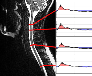
Figure 2. Subject 1: selected spinal cord locations (a) with corresponding flow rate variation obtained from PC-MRI measurements (b) and from model predictions for  $\mathcal {R}=4.78$ (c), $\mathcal {R}=0$ (d), $\mathcal {R}=1$ (e) and $\mathcal {R}=20$ ( f), with associated normalized stroke volumes shown in (g).

Figure 3. Subject 2: selected spinal cord locations (a) with corresponding flow rate variation obtained from PC-MRI measurements (b) and from model predictions for  $\mathcal {R}=4.78$ (c), $\mathcal {R}=0$ (d), $\mathcal {R}=1$ (e) and $\mathcal {R}=20$ ( f), with associated normalized stroke volumes shown in (g).
With the uniform values  $\hat {\gamma }=1$ and $\mathcal {R} = 4.78$ selected in the computations, the comparisons in figures 2 and 3 indicate that the model is able to describe reasonably well the main features of the pulsating flow rate, including its particular shape and the phase lag of its peak value. In addition, the streamwise decay of the stroke volume (figures 2g and 3g), a metric often used in the medical community to characterize CSF flow, is seen to agree well with the corresponding values computed from the MRI data, with root-mean-square differences between model and MRI remaining below 0.09 for both subjects. As a further consistency check, one may use the measured value of $V_{S}(0)$ along with the accompanying dimensionless prediction $\hat {V}_{S}(0)$ to obtain from the definition $V_{S}(0)=\gamma _o L \Delta p \hat {V}_{S}(0)$ an estimate for the mean fluctuation amplitude $\Delta p$. The value obtained, $\Delta p=73$ Pa for subject 1 and $\Delta p=80$ Pa for subject 2, corresponding to a peak-to-peak value of approximately 200 Pa, is well within the range of values reported in the literature (Eide & Brean Reference Eide and Brean2006), thereby providing additional confidence in the model.
To investigate the sensitivity of the model predictions to changes in trabeculae resistance, results for varying  $\mathcal {R}$ are also included in figures 2 and 3. In the absence of trabeculae, i.e. for $\mathcal {R}=0$, both the rate at which the flow rate fluctuation decays along the canal and the general flow rate waveform, including the associated phase lag, are in poor agreement with the MRI measurements. Consequently, for $\mathcal {R}=0$ the modelled streamwise decay of stroke volume, shown in figures 2( $g$) and 3( $g$), is also seen to strongly overpredict the amount of CSF flow in the thoracic and lumbar regions compared with the MRI measurements. These quantitative findings emphasize the important effects of trabeculae, previously pointed out by Tangen et al. (Reference Tangen, Hsu, Zhu and Linninger2015). As can be seen in figures 2 and 3, the results are not very sensitive to the specific choice of $\mathcal {R}$, provided that an order-unity value is selected. Nevertheless, the computations obtained with $\mathcal {R} = 4.78$, the value determined using the permeability and other anatomical features taken from the literature (Tada & Nagashima Reference Tada and Nagashima1994; Stockman Reference Stockman2006; Gupta et al. Reference Gupta, Soellinger, Boesiger, Poulikakos and Kurtcuoglu2009), appear to give better overall agreement with the MRI measurements, providing the optimal amount of attenuation all along the canal.
5. Concluding remarks
The temporal and spatial variation of the flow rate predicted by the one-dimensional model developed here supplemented with a presumed ICP waveform has been shown to predict the main features revealed in in vivo experiments. Utilization of the model in future efforts to develop non-invasive measurements of ICP requires the solution of the inverse problem, i.e. the computation of the ICP fluctuation from the PC-MRI flow measurements. Given the uncertainty regarding the canal compliance and the trabeculae-network properties, it is unclear whether conventional parameter-fitting approaches will be successful in these future developments or whether more elaborate optimization algorithms, possibly based on machine-learning techniques, will be needed. In improving the model, these future efforts should also account for localized pressure losses associated with the presence of additional spinal microstructures, such as nerve roots and ligaments.
Funding
The work of S.C., V.H. and A.L.S. was supported by the National Institute of Neurological Disorders and Stroke through contract no. 1R01NS120343-01. The work of W.C. was supported by the Comunidad de Madrid through the contract CSFFLOW-CM-UC3M. C.M.B., C.G. and W.C. acknowledge the support of the Spanish MICINN through the coordinated project PID2020-115961RB. C.M.B. and C.G. also acknowledge the support provided by Junta de Andalucía and European Funds through grant P18-FR-4619.
Declaration of interests
The authors report no conflict of interest.


 Open access