


1. Introduction
From flagellar beating of spermatozoa to water-walking insects, from the wave-like lateral flexions of fish to flying, nature has evolved myriad strategies for locomotion and propulsion in fluidic environments (Hu, Chan & Bush Reference Hu, Chan and Bush2003; Bush & Hu Reference Bush and Hu2006; Bühler Reference Bühler2007; Gaffney et al. Reference Gaffney, Gadêlha, Smith, Blake and Kirkman-Brown2011; Eloy Reference Eloy2012; Smits Reference Smits2019). A perhaps lesser-known propulsion mechanism is enacted by honeybees (Apis mellifera) trapped on the surface of water: in oscillating its wings, the bee generates a fore–aft asymmetric wave field that contributes to forward motion (Roh & Gharib Reference Roh and Gharib2019). Inspired by the stricken honeybee, Rhee et al. (Reference Rhee, Hunt, Thomson and Harris2022) designed SurferBot: a centimetre-scale interfacial robot that achieves wave-driven locomotion speeds of around  $1\ {\rm cm}\ {\rm s}^{-1}$ by inducing asymmetric vibrations with a small eccentric-mass motor mounted on SurferBot's back. Wave-driven propulsion may also be realized by designing floating bodies with mass- and/or geometric-asymmetries that generate thrust and torques by exchanging momentum with waves generated by the object as it oscillates on the free surface of a globally vibrating fluid bath (Barotta et al. Reference Barotta, Thomson, Alventosa, Lewis and Harris2023; Ho et al. Reference Ho, Pucci, Oza and Harris2023; Oza et al. Reference Oza, Pucci, Ho and Harris2023). At much larger scales, Benham et al. (Reference Benham, Devauchelle, Morris and Neufeld2022) achieved wave-driven locomotion speeds of around $1\ {\rm m}\ {\rm s}^{-1}$ by forcing a canoe into oscillations by jumping up and down on its gunwales, a technique known as gunwale bobbing. In this case a simple wave-equation model was derived by treating the canoe as an oscillating pressure source with a prescribed motion, ignoring the effects of dispersive waves and considering an idealized Gaussian canoe shape. Although outside the scope of the present work, other studies have investigated alternative routes to wave-driven propulsion including symmetry-breaking due to the presence of boundaries (Tarr et al. Reference Tarr, Brunner, Soto and Goldman2024) and using acoustic radiation forces (Sabrina et al. Reference Sabrina, Tasinkevych, Ahmed, Brooks, Olvera de la Cruz, Mallouk and Bishop2018; Roux, Martischang & Baudoin Reference Roux, Martischang and Baudoin2022; Martischang, Roux & Baudoin Reference Martischang, Roux and Baudoin2023).
Based on classical results (Longuet-Higgins & Stewart Reference Longuet-Higgins and Stewart1964; Longuet-Higgins Reference Longuet-Higgins1977), the prevailing opinion is that the thrust necessary to drive locomotion originates from an asymmetric radiation of wave momentum (Rhee et al. Reference Rhee, Hunt, Thomson and Harris2022; Ho et al. Reference Ho, Pucci, Oza and Harris2023; Oza et al. Reference Oza, Pucci, Ho and Harris2023). A scaling argument for two-dimensional wave-driven propulsion (i.e. restricted to the vertical plane) is as follows: consider a body of length  $L$ oscillating at the interface of a fluid with density $\rho$ and kinematic viscosity $\nu$ in the presence of gravity $g$. If the oscillations have amplitude $A$, frequency $\omega$ and wavenumber $k$, the thrust due to oscillating waves (per unit width) scales as
 \begin{equation} F_T\sim{\rho v^2/k},\end{equation}
where  $v=A\omega$ is the speed associated with the oscillations (Longuet-Higgins & Stewart Reference Longuet-Higgins and Stewart1964). This assumes that the fluid pressure applies over a distance ${\sim }1/k$. Forward motion at speed $U$ results in an inertial drag force that scales as
 \begin{equation} F_D\sim\rho C_DU^2L,\end{equation}
where  $C_D$ is a drag coefficient, and both (1.1) and (1.2) have the dimensions of a force per unit width ( ${\rm N}\ {\rm m}^{-1}$). By considering a number of known examples of wave-driven propulsion (figure 1), we demonstrate that thrust (1.1) balances drag (1.2) with a ratio of 0.001–0.1, indicating the range of prefactor values associated with (1.1).

Figure 1. Thrust scaling  $F_T$ (1.1) plotted against drag scaling $F_D$ (1.2) for a variety of different bodies oscillating at the water surface (forces are taken as per unit width). Parameter values for each case are given in table 1 in Appendix A. We observe that thrust balances drag with a ratio of 0.001–0.1, which is consistent with oscillation-induced propulsion predicted by our mathematical model.
Table 1. Parameters used in figure 1 and their references. The type of fluid in all cases is water, for which  $\rho =1000\ {\rm kg}\ {\rm m}^{-3}$, $\gamma =0.073\ {\rm N}\ {\rm m}^{-1}$, $\nu =10^{-6}\ {\rm m}^2\ {\rm s}^{-1}$, except the capillary surfer, for which the fluid is a water–glycerol mixture and the parameters are $\rho =1176\ {\rm kg}\ {\rm m}^{-3}$, $\gamma =0.0664\ {\rm N}\ {\rm m}^{-1}$ and $\nu =1.675\times 10^{-5}\ {\rm m}^2\ {\rm s}^{-1}$. The frequency is $f=\omega /2{\rm \pi}$.

Whilst the foregoing scaling argument performs well in capturing the thrust–drag balance, it fails to provide further insight into the problem. For example, there is no way of predicting the prefactors of the scalings or the related efficiency of propulsion. Further, without a model of the wave field, momentum conservation cannot be verified. We herein present a theoretical model for wave-driven propulsion in the case of a raft floating at the fluid interface undergoing small-amplitude oscillations due to an external force. The equations of motion for the raft are coupled to a quasipotential flow model of the fluid dynamics (Dias, Dyachenko & Zakharov Reference Dias, Dyachenko and Zakharov2008). Propulsion is demonstrated in the form of a constant drift speed that results from a time-averaged thrust force due to the oscillations. We compare our predictions for the wave field and raft motion with the experimental data of SurferBot (Rhee et al. Reference Rhee, Hunt, Thomson and Harris2022), and then use our model to optimize the efficiency of propulsion by varying the frequency of vibrational forcing and the position at which the forcing is applied. Some possible extensions and applications of our model to insect locomotion and competitive water sports are discussed in conclusion.
2. Theoretical model for an oscillating raft
Whilst scaling arguments for wave-driven propulsion show some success in predicting drag and thrust (see figure 1), there is no existing theory to model wave-driven dynamics that in turn can be used quantitatively to predict and maximize the efficiency of propulsion. In the following section we build such a model, first by formulating the equations of motion for a floating raft in two dimensions, then by accounting for the coupled fluid flow problem using quasipotential flow theory.
2.1. Equations of motion for the raft
Let us consider a two-dimensional body of fluid with the horizontal and vertical coordinates given by  $x$ and $z$, respectively. A floating raft of length $L$ resting on the fluid surface is subject to an applied periodic force $\boldsymbol {F}_A=(F_{A,x}(t),F_{A,z}(t))$ imposed at position ${\boldsymbol {x}}_A = (x_A, z_A)$ measured from the raft centre of mass (figure 2a,b). In response to $\boldsymbol {F}_A$ it is assumed that the centre of mass of the raft $\boldsymbol {X}$ undergoes small oscillations in the $x$ and $z$ directions, whilst translating horizontally with an a priori unknown constant drift speed $U$. The action of $\boldsymbol {F}_A$ also induces a torque that gives rise to oscillations in the $x\unicode{x2013}z$ plane, the rotation vector given by $\boldsymbol {\theta }=\theta (t) {\boldsymbol {j}}$ where the unit vector ${\boldsymbol {j}}$ points out of the page.

Figure 2. (a) A raft of length  $L$ oscillating on the surface $z = \eta (x,t)$ of a fluid of resting depth $H$ self-propels with a drift velocity $U$ thanks to a self-generated wave field. (b) Schematic diagram of the raft dynamics (in the moving frame). The raft is subject to an oscillatory external force $\boldsymbol {F}_A = (F_{A,x}(t), F_{A, z}(t))$ applied at position $x_A$ (in the frame of the raft). The applied force gives rise to small horizontal and vertical oscillations $\xi (t)$ and $\zeta (t)$, in addition to planar rotations with angle $\theta (t)$.
The equations of motion (in the moving frame) for the position and orientation of the centre of mass of the raft are
 \begin{gather} m\ddot{\boldsymbol{X}} = \boldsymbol{F}_A + \int_S (p-p_a) \boldsymbol{n} \, \mathrm{d}\kern0.7pt x - \boldsymbol{F}_D, \end{gather}
 \begin{gather}I \ddot{\boldsymbol{\theta}} = {\boldsymbol{x}}_A\times \boldsymbol{F}_A + \int_S (p-p_a) \boldsymbol{x}\times \boldsymbol{n} \, \mathrm{d}\kern0.7pt x , \end{gather}
where  $m$ is the mass (per unit width) of the raft and $I=m L^2/12$ is the moment of inertia of the raft (per unit width), taken as the value for a rod rotating about its centre of mass. The second term on the right-hand side of (2.1a) is the force arising from fluid pressure, $p$, minus its atmospheric value $p_a$, where the vector $\boldsymbol {n}$ is the unit normal to the raft surface, $S$, pointing in the positive $z$ direction. The drag force, which ultimately results from viscous friction along the hull (see Appendix B), is approximated using an empirical drag coefficient such that
 \begin{equation} \boldsymbol{F}_D=\tfrac{1}{2}C_D \rho L |\dot{{\boldsymbol{X}}}|\dot{{\boldsymbol{X}}}.\end{equation}
The torques on the right-hand side of (2.1b) are those arising from their corresponding forces in (2.1a). Drag on rotational motion is assumed to be negligible. We note the omission of a gravitational term in (2.1a) which is balanced by the pressure integral term in the steady state. While we do not go into detail, the steady contribution to the pressure is a combination of surface tension (acting at the edges of the raft) and Archimedes buoyancy. We assume that the mass of the raft is such that this balance is sustained and hence we ignore the gravitational term from the momentum equation (2.1a).
The experiments of Rhee et al. (Reference Rhee, Hunt, Thomson and Harris2022) use an eccentric-mass motor to oscillate the raft. We therefore take  $\boldsymbol {F}_A$ to be periodic, specifically
 \begin{equation} (F_{A,x},F_{A,z})= (\hat{F}_{A,x},\hat{F}_{A,z}) {\rm e}^{i\omega t}, \end{equation}
where  $\hat {F}_{A,x}$, $\hat {F}_{A,z}$ are small complex constants (incorporating both amplitude and phase) – the real part is assumed for (2.3) and all other complex expressions. In response, the position of the centre of mass of the raft is
 \begin{equation} {\boldsymbol{X}}=(X(t),Z(t))=(U t + \xi(t),\zeta(t)), \end{equation}
where
 \begin{equation} (\xi,\zeta)= (\hat{\xi},\hat{\zeta}){\rm e}^{i\omega t},\quad \hat{\xi},\hat{\zeta}\in\mathbb{C}, \end{equation}
represent small horizontal and vertical oscillations, respectively (figure 2b). The profile of the raft is thus described by
 \begin{equation} z=Z(t)+(x-X(t))\tan \theta(t)\quad\mathrm{on}:\quad |x-X(t)|\leqslant L/2, \end{equation}
where
 \begin{equation} \theta= \hat{\theta}{\rm e}^{i\omega t},\quad \hat{\theta}\in\mathbb{C}. \end{equation}
Likewise, the fluid pressure reads
 \begin{equation} p = p_a + \hat{p} {\rm e}^{i\omega t}, \end{equation}
where  $\hat {p} = \hat {p}(x, z)$ is a complex function.
Before going further, we pause to discuss the steady drift speed,  $U$. The hypothesis of this paper is that steady drift is a result of a balance between the propulsion due to waves and the resultant inertial drag. We propose that the propulsion due to waves is given by the time-averaged $x$ component of the pressure integral term in (2.1a) and that this thrust force is given by
 \begin{equation} {\bar{F}}_{T}=\overline{\int_S(p-p_a)\left( \boldsymbol{n}\boldsymbol{\cdot}\boldsymbol{i} \right) \mathrm{d}\kern0.7pt {x}}, \end{equation}
where  $\boldsymbol {i}$ is a unit vector in the horizontal and the overhead-bar notation denotes the time-average over one oscillation period $T=2{\rm \pi} /\omega$, which is $({1}/{T})\int _0^{T} \cdot \, \mathrm {d}t$. As shown in Appendix B, the time-average of the drag term (2.2) is well-approximated by the component due to steady drift $U$, while drag due to oscillations is comparatively small. Hence, the drag in the $x$ direction approximates to
 \begin{equation} {\bar{F}}_{D}\approx \tfrac{1}{2}C_D \rho L U^2.\end{equation}
The time-averaged drag in the vertical direction is ignored, as discussed in Appendix B. Hence, we write  $\bar {\boldsymbol {F}}_{D}\boldsymbol {\cdot } \boldsymbol {i}=\bar {F}_D$ to simplify notation. Since the drag term (2.10) is approximately the same as it would be for steady flow past the raft, we use Blasius’ theory of flow past a flat plate to estimate $C_D=1.33\times{Re}^{-1/2}$ in terms of the Reynolds number $Re =UL/\nu$ (Schlichting & Gersten Reference Schlichting and Gersten2016).
From the above analysis, it is clear that the time-averaged thrust (2.9) and drag forces (2.10) are both second order, that is, proportional to the square amplitude of the oscillation. In other words, if the relative magnitude of the applied force compared with Archimedes buoyancy is represented by a small parameter  $\epsilon =|\boldsymbol {F}_A|/\rho g L^2$, then we say that $\hat {F}_{A,x},\hat {F}_{A,z}=O(\epsilon )$, and hence ${\bar {F}}_{D},{\bar {F}}_{T}=O(\epsilon ^2)$ are second-order phenomena. Consequently, by taking a square-root of the thrust–drag balance ( ${\bar {F}}_{T}={\bar {F}}_{D}$), we see that $U=O(\epsilon )$. For example, in the case of SurferBot studied later, we find $\epsilon \approx 0.18$ and hence $\epsilon ^2\approx 0.032$.
To fully determine  $U$ by equating (2.9) and (2.10) requires a fluid dynamics model for the pressure $p$ in (2.9). Likewise, the fluid pressure determines the first-order dynamics of the raft. Specifically, after substituting (2.3), (2.5a,b), (2.7a,b) and (2.8) into (2.1) and linearizing, the first-order oscillating dynamics (in the moving frame) are described by
 \begin{gather} -m\omega^2 {\hat{\xi}}= \hat{F}_{A,x}, \end{gather}
 \begin{gather}-m\omega^2 {\hat{\zeta}}=\hat{F}_{A,z} + \int_{{-}L/2}^{L/2} \hat{p}|_{{z}=0} \, \mathrm{d}\kern0.7pt {x}, \end{gather}
 \begin{gather}-\frac{L^2}{12}m\omega^2 \hat{\theta}= {x}_A\hat{F}_{A,z} + \int_{{-}L/2}^{L/2} x\hat{p}|_{{z}=0} \, \mathrm{d}\kern0.7pt {x}. \end{gather}
Equations (2.11) provide a relationship between the constants  $\hat {F}_{A,x},\hat {F}_{A,z}$, ${x}_A$ and the constants $\hat {\xi },\hat {\zeta },\hat {\theta }$, given $\hat {p}$ calculated by formulating the corresponding fluid flow problem.
2.2. Quasipotential flow
The body of fluid is assumed to be irrotational and infinitely wide with a finite depth  $H$ and a free surface at $z=\eta (x,t)$, such that $-\infty < x<\infty$ and $-H\leqslant z\leqslant \eta$. Following the approach of Dias et al. (Reference Dias, Dyachenko and Zakharov2008), the velocity for a weakly damped flow can still be modelled as the gradient of a potential function $\phi (x,z,t)$ to good approximation. We choose to include viscosity in our model so as to replicate the spatial decay in waves observed in experiments. Due to incompressibility, $\phi$ satisfies
 \begin{equation} \nabla^2\phi=0.\end{equation}
The linearized kinematic condition applies on the water surface, such that
 \begin{equation} \phi_z=\eta_t-2\nu \eta_{xx}:\quad\mathrm{on}\ z=0.\end{equation}
On the raft the linearized kinematic condition takes the form
 \begin{equation} \phi_z =\dot{\zeta}+x\dot{\theta} :\quad\mathrm{on}\ z=0,\quad |x-X|\leqslant L/2.\end{equation}
In addition, the unsteady version of Bernoulli's equation applies within the fluid which, upon linearization, becomes
 \begin{equation} \phi_t + gz +\frac{p}{\rho} +2\nu \phi_{zz}=\frac{p_a}{\rho}. \end{equation}
After applying the dynamic boundary condition  $p-p_a=-\gamma \eta _{xx}$ on the free surface, (2.15) yields
 \begin{equation} \phi_t + g\eta - \frac{\gamma}{\rho}\eta_{xx}+2\nu \phi_{zz}=0:\quad\mathrm{on}\ z=0,\quad |x-X|> L/2, \end{equation}
where Laplace pressure introduces the surface tension  $\gamma$. Finally, the bottom surface is impermeable, such that
 \begin{equation} \phi_z= 0:\quad\mathrm{on}\ z={-}H. \end{equation}
In the same manner as § 2.1, we seek solutions of the form  $\phi = \hat {\phi } {\rm e}^{{i}\omega t}$, $\eta = \hat {\eta } {\rm e}^{{i}\omega t}$, where $\hat {\phi } = \hat {\phi }(x,z)$, $\hat {\eta } = \hat {\eta }(x)$ are complex functions.
Henceforth, we formulate the fluid flow problem in the moving reference frame,  $x\rightarrow x+Ut$. However, we restrict our attention to the case where the drift speed is much smaller than the typical wave speed, such that $U\ll \sqrt {gL}$. In this way, we focus on the flow resulting from the oscillations, rather than the drift velocity.
The boundary conditions (2.13), (2.14), (2.16) and (2.17) are combined with (2.12) to give the governing system
 \begin{gather} {\nabla}^2\hat{\phi}=0, \end{gather}
 \begin{gather}\hat{\phi}_{z}=\frac{\gamma}{\rho g} \hat{\phi}_{zxx}+\frac{\omega^2}{g}\hat{\phi}+\frac{4i \nu \omega}{g} \hat{\phi}_{xx} :\quad\mathrm{on}\ z=0,\quad |x|> L/2, \end{gather}
 \begin{gather}\hat{\phi}_{z}={i}\omega(\hat{\zeta}+x\hat{\theta}):\quad\mathrm{on}\ z=0,\quad |x|\leqslant L/2, \end{gather}
 \begin{gather}\hat{\phi}_{x}={\pm} {i} k\hat{\phi} :\quad\mathrm{on}\ x={\mp} \ell, \end{gather}
 \begin{gather}\hat{\phi}_{z}= 0:\quad\mathrm{on}\ z={-}H. \end{gather}
For the purpose of numerical simulation, the domain is rendered finite of length  $2\ell$ in the $x$ direction. Radiative boundary conditions (2.18d) are chosen at the left- and right-hand boundaries to avoid reflection, where $k$ satisfies the dispersion relation
 \begin{equation} \omega^2=k\tanh kH\left( g+\frac{\gamma}{\rho} k^2 \right) +4{i}\nu \omega k^2.\end{equation}
The final step in linking together the fluid–raft interaction is calculating the thrust force  ${\bar {F}}_T$ (2.9) in terms of the pressure and normal vector, noting that to leading order $\boldsymbol {n}\boldsymbol {\cdot }\boldsymbol {i}\approx -{\eta }_{x}$. From (2.15) the pressure on the raft is given by
 \begin{equation} \hat{p} ={-}\rho({i}\omega \hat{\phi} +g \hat{\eta}+ 2\nu \hat{\phi}_{zz})|_{z=0}.\end{equation}
Meanwhile, on the free surface the wave field is given by the solution to the kinematic condition (2.13), such that
 \begin{equation} {i}\omega\hat{\eta}-2\nu\hat{\eta}_{xx}=\hat{\phi}_{z}|_{z=0},\end{equation}
which is accompanied by radiative boundary conditions (similar to (2.18d)) at  $x=\mp \ell$ and continuity boundary conditions on the raft, namely $\hat {\eta }=\hat {\zeta }\pm \hat {\theta }L/2$ on $x=\pm L/2$.
2.3. Summary
Let us now summarize the governing system of equations. Given constants  $\hat {F}_{A,x}$, $\hat {F}_{A,z}$ and $x_A$, the dynamics of the raft are determined by (2.11), coupled to the fluid flow problem given by (2.18) via the pressure (2.20). The drift speed $U$ is then calculated by equating thrust (2.9) and drag (2.10), where ${\bar {F}}_T$ follows from the solution via $\hat {p}$ and $\hat {\eta }$. The problem is solved numerically in MATLAB using a combination of finite differences to solve the PDE system (2.18) and Newton's method to resolve the coupling with (2.11). A large numerical domain is used, $\ell,H\gg L$, such that the solution does not depend on $\ell$ and $H$. Example code is provided in the supplementary materials available at https://doi.org/10.1017/jfm.2024.352.
3. Model results, validation and application to SurferBot
We begin this section by exploring the numerical results of our model, demonstrating that it satisfies a momentum balance. We then consider a specific application of our model to SurferBot (Rhee et al. Reference Rhee, Hunt, Thomson and Harris2022) comparing our results directly with experimental data.
3.1. Numerical results and momentum balance
Motivated by large-scale examples of bodies oscillating at the water surface (Benham et al. Reference Benham, Devauchelle, Morris and Neufeld2022), as a simple demonstration of the fluid flow problem, we solve (2.18) numerically in the case of a 1-m-long raft oscillating at 1 Hz on the surface of water ( $\rho =1000\ {\rm kg}\ {\rm m}^{-3}$, $\gamma =0.073\ {\rm N}\ {\rm m}^{-1}$, $\nu =10^{-6}\ {\rm m}^{2}\ {\rm s}^{-1}$). For the sake of simplicity we restrict our attention to pure pitching ( $\hat {\zeta }=0$) and pure heaving (
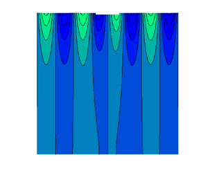
 $\hat {\theta }=0$), ignoring in the first instance the coupling to the forcing constants in (2.11). The velocity potential is plotted in figure 3 in the case of pure pitching (figure 3a) and pure heaving (figure 3b). As anticipated, $\bar {F}_T=0$ for both these cases since both heaving and pitching are required to generate thrust. Although both heaving and pitching are required to generate thrust in the case of vanishingly small drift velocity, it is not clear if this remains true at large drift velocities in general (Benham et al. Reference Benham, Devauchelle, Morris and Neufeld2022).

Figure 3. Velocity potential (taken as the imaginary part rescaled by  $\omega L^2$) in the case of (a) pure pitching $\hat {\zeta }/L=0,\hat {\theta }=0.1,$ and (b) pure heaving $\hat {\zeta }/L=0.01,\hat {\theta }=0$, of a 1-m-long raft oscillating at 1 Hz on the surface of water.
Next, we validate our numerical scheme using a momentum balance. As shown in Appendix C and first discussed by Longuet-Higgins & Stewart (Reference Longuet-Higgins and Stewart1964), an expression for the thrust force can be derived via integration of the Euler equations. This results in an equivalence between  $\bar {F}_T$ and the momentum flux of the form
 \begin{equation} {\bar{F}}_T=\left[\overline{\int_{{-}H}^{\eta}\left (\rho u^2 + p\right)\mathrm{d}z}\right]^{x={-}\ell}_{x=\ell}.\end{equation}
The term on the right-hand side is the difference in mean momentum-flux between backward and forward directions (including the pressure difference). Hence, when larger waves propagate backwards than forwards, this results in a positive thrust. In Appendix C we show how to calculate this balance when surface tension and viscosity are neglected. Calculating the left- and right-hand sides of (3.1) numerically for a range of  $\omega$ yields very close agreement between the two (figure 4), giving us confidence that the numerical scheme is accurate and consistent with global momentum conservation.

Figure 4. Comparison between the numerically calculated thrust  ${\bar {F}}_T$ and momentum flux across the domain (3.1) showing close agreement between the two. Comparison is also made with the scaling proposed by Longuet-Higgins (see Appendix C) exhibiting only qualitative agreement. Surface tension and viscosity are neglected for the purpose of these calculations.
It should be noted that whilst our model accurately conserves momentum, it neglects any possible contribution to thrust from vortex shedding since the fluid is considered irrotational. It is well known that some forms of insect locomotion rely on both vortex shedding and capillary wave propagation (Bush & Hu Reference Bush and Hu2006; Bühler Reference Bühler2007). To incorporate thrust from any vortices generated by the motion would require a model for rotational fluid flow, which we leave for a future study. However, by comparing our model with SurferBot in the next section, we will see that our predictions perform well despite neglecting vorticity, suggesting that in the present case vortices are not the leading-order driver of propulsion (Barotta et al. Reference Barotta, Thomson, Alventosa, Lewis and Harris2023).
3.2. Comparison with SurferBot
To demonstrate a specific application of our model, we calculate the dynamics of SurferBot (Rhee et al. Reference Rhee, Hunt, Thomson and Harris2022), for which dimensional parameter values are given in table 1 in Appendix A. In this case, the force is applied via an eccentric-mass motor positioned at  $x_A=-3\ {\rm mm}$ from the centre of the raft. The forces $F_{A,x}$, $F_{A,z}$, are assumed to be out of phase, and are estimated using a scaling law relating the mass (per unit width) of the raft $m=2.6\ {\rm g}/3\ {\rm cm}$ and the oscillation amplitude $A=150\ {\mathrm {\mu }}{\rm m}$, such that
 \begin{equation} (\hat{F}_{A,x},\hat{F}_{A,z}) = m\omega^2A(i,1).\end{equation}
Our model predicts a drift speed of  $U\approx 2\ {\rm cm}\ {\rm s}^{-1}$, compared with an experimentally measured speed of ${\sim }1.8\ {\rm cm}\ {\rm s}^{-1}$. This may suggest that Blasius’ theory for the drag coefficient on a flat plate, $C_D=1.33\times {Re}^{-1/2}$, may underestimate the drag for SurferBot, with $C_D=1.75\times {Re}^{-1/2}$ giving the best fit.
A comparison between the experimental and theoretical self-generated wave field is plotted in figures 5(a) and 5(b), whilst the time-varying position of the back and front of SurferBot are shown in figures 5(c,e) (experimental) and 5(d,f) (theoretical). Overall, the results of our theoretical model exhibit good qualitative agreement with experiments and yield an excellent prediction of the drift speed,  $U$. However, there is disagreement in the amplitude of the wave field and hence the oscillation amplitude of SurferBot, in addition to the decay length scale of the waves. However, these discrepancies are likely attributed to some obvious differences between experiment and theory, including the precise form of the oscillatory forcing (eccentric-mass motor in experiments versus a periodic point-force in the theory), three-dimensional effects of both the SurferBot geometry and wave field or indeed the flexure of the SurferBot body contributing to wave damping.

Figure 5. Comparison between the experimental wave amplitude from (a) SurferBot and (b) the mathematical model. In (b), the theoretical wave amplitude (red) is scaled by  $\sqrt {2L/{\rm \pi} x}$ to be consistent with the far-field behaviour of Bessel functions (since in practice the waves extend radially to the far-field). The unscaled wave amplitude is shown as a dotted black line. (c–f) Comparison between the experimental and theoretically predicted position of the (c,d) aft and (e,f) fore. (d,f) In the theoretical predictions, $\boldsymbol {x}_{aft}=\boldsymbol {X}-(1/2,\theta /2)L$ and $\boldsymbol {x}_{fore}=\boldsymbol {X}+(1/2,\theta /2)L$. Experimental data reproduced with permission.
4. Efficiency and optimization
Furnished with a theoretical model describing the SurferBot dynamics, we can interrogate the efficiency of propulsion and optimize the parameters of SurferBot thereafter. The efficiency of propulsion is given in terms of the applied and useful (propulsive) power. The total applied power is given by
 \begin{equation} {\bar{P}}_{A}= \overline{{F}_{A,z}\dot{\zeta}}+x_A \overline{F_{A,z}\dot{\theta}} , \end{equation}
the sum of linear and angular contributions. There is also a contribution  $\overline {{F}_{A,x}\dot {\xi }}$ to ${\bar {P}}_{A}$ which vanishes because ${F}_{A,x}$ and $\dot {\xi }$ are out of phase due to (2.11a). The propulsive power is taken as $\bar {P}_T= \bar {F}_T U$ and the efficiency is defined as $\chi =\bar {P}_T/\bar {P}_{A}$. Hence, in the case of SurferBot (before optimization), we calculate an efficiency value of $\chi =1.8\,\%$ from our mathematical model.
The two parameters we attempt to optimize are the driving frequency  $\omega /2{\rm \pi}$ and the horizontal position of the forcing, $x_A$. We assume that the horizontal force $\hat {F}_{A,x}=0$ (as it does not contribute to forward thrust anyway) and that the total power (4.1) is fixed at the value calculated for SurferBot, $\bar {P}_{A}=7.2\times 10^{-4}\ {\rm W}\ {\rm m}^{-1}$. Note that the applied force $\hat {F}_{A,z}$ must change to maintain constant power at variable frequency. Efficiency is plotted as a function of $\omega /2{\rm \pi}$ and $x_A$ in figure 6(a,b) showing an optimum frequency of 16 Hz and an optimum motor position of 5 mm behind the raft centre, both of which could be readily tested in a future experiment.

Figure 6. (a,b) Optimization of SurferBot efficiency  $\chi$ by varying the frequency and the motor position whilst maintaining constant total applied power $\bar {P}_{A}$. The optimum values (illustrated with black dots) are the outcome of a two-parameter optimization, and hence the plotted curves are slices of the two-dimensional efficiency surface at its maximum.
A possible interpretation of the optimum frequency is a resonance between the raft and the fluid, which occurs at the natural frequency  $f$ (e.g. for heaving or pitching motion). This scales as $f\sim ({g}/{L})^{1/2}$, producing a natural frequency of around ${\sim }14$ Hz in the case of SurferBot. The optimum position simply scales with the length of the raft $x_A\sim L$, but the precise value may result from a trade-off between exciting the natural frequencies associated with heaving and pitching (i.e. by forcing at either the middle or the end of the raft, respectively).
In a similar manner to the discussion in § 1, it is also possible to derive an estimate of efficiency using scaling arguments. To do so we may assume that the total power  $\bar {P}_A$ (4.1) can be split into the contribution from propulsive power, which scales as $\bar {P}_T\sim \bar {F}_T U$, and the power radiated away by the waves (front and back), which scales as $\bar {P}_{{wave}}\sim 2\bar {F}_T c_g$, where $c_g=\mathrm {d}\omega /\mathrm {d}k$ is the group velocity of the waves. The efficiency then scales as
 \begin{equation} \chi\sim \frac{{Ma}}{2+{Ma}},\end{equation}
where  ${Ma}=U/c_g$ is the Mach number. In the case of SurferBot we find that (4.2) yields $\chi \sim 1.81\,\%$, which is in very close agreement with the model calculation $\chi =1.8\,\%$. The above scaling also compares well with a range of SurferBot simulations at small Mach numbers between ${Ma}=10^{-3}\unicode{x2013}10^{-1}$, which is expected since our model assumes a vanishingly small drift velocity. However, such a scaling argument obviously provides no means for optimization. Nevertheless, it indicates that efficiency increases with Mach number, which is probably due to a decrease in forward-propagating waves as the motion approaches ${Ma}=1$ (which we discuss further shortly).
5. Discussion and perspectives
Using linear quasipotential flow theory, coupled with the equations of motion for an oscillating raft, we have demonstrated how the raft propels itself forward using its own waves. The close agreement between our linear model and the experimental data of SurferBot (Rhee et al. Reference Rhee, Hunt, Thomson and Harris2022) indicates that we have captured the key physics at play for this self-propelling centimetre-scale robot. Nevertheless, there are several further improvements to the model that are worth discussing.
The assumption of a vanishingly small drift velocity is worth revisiting. In a future study a finite drift speed could be incorporated into the fluid-flow problem. This would require transforming equations (2.18) to a moving reference frame, thereby introducing new derivative terms of the potential. Consequently, the dispersion relation (2.19) would need to be modified and may result in multiple-wavenumber solutions for forward and backward travelling waves. An initial resolution to this problem could involve studying a small but finite drift speed using the method of asymptotic expansions.
A finite drift speed incorporated into the model would result in a Doppler-shifted wave field, as discussed by Benham et al. (Reference Benham, Devauchelle, Morris and Neufeld2022). In this case, a key dimensionless parameter is the Mach number, Ma, which is defined as the ratio between the drift speed  $U$ and the group velocity of the waves $c_g$. The Mach number is closely related to whether or not forward (in addition to backward) waves are propagated. Specifically, if the drift speed is larger than the wave speed for a particular wavenumber, this indicates that such a wave can only propagate behind the object and not in front of it. Since the momentum balance (3.1) indicates that larger forward waves reduce the forward thrust, we would expect more efficient motion at higher Mach numbers (which is consistent with the scaling (4.2)). The value of the Mach number and hence the shape of the wave field varies considerably for different cases of wave-driven propulsion. For example, the wave field of SurferBot ( ${Ma}=0.04$) is markedly different to that of gunwale bobbing on a paddleboard ( ${Ma}=1.7$). The former produces significant waves both forwards and backwards, whereas the latter has purely backward waves (e.g. compare figure 3a of Rhee et al. (Reference Rhee, Hunt, Thomson and Harris2022) with figure 1a of Benham et al. (Reference Benham, Devauchelle, Morris and Neufeld2022)). Note that the Mach number is defined slightly differently from Benham et al. (Reference Benham, Devauchelle, Morris and Neufeld2022), who used the phase velocity $c_p$ rather than the group velocity $c_g$ in the denominator, resulting in different quoted values.
By considering a finite drift speed, one can then study how symmetry is broken when oscillations commence (i.e. the start-up problem for wave-driven propulsion). One could investigate, for example, how perturbations grow or decay from a stationary state when subjected to oscillations. This would then help determine the necessary conditions for initiating forward propulsion under different operating conditions. Therein lie numerous optimization problems, such as the optimal control of a single oscillator (or multiple oscillators) with variable positions or masses, not to mention the optimization of the shape of the raft itself. One could also consider different optimization objectives, such as maximizing speed as well as efficiency.
Whilst the present irrotational model compares well with the SurferBot data, it is nevertheless desirable to determine for which cases the irrotational assumption breaks down. To do so would require either a rotational fluid model, such as a direct numerical simulation, or a particle image velocimetry experiment to capture the velocity field of the fluid around the SurferBot as it moves (Chu & Fei Reference Chu and Fei2014). These approaches, which both lie outside the scope of this study, would reveal the strength of the vorticity in the vicinity of the raft, as well as the contribution towards the propulsion and drag forces. For example, it is well known that vortices play a significant role in the locomotion of water striders which are smaller and faster than SurferBot (Bühler Reference Bühler2007). However, at larger scales (e.g. in the case of gunwale bobbing) it is not known what role vorticity plays.
We suspect that the largest source of error in our model may come from neglecting the three-dimensional nature of SurferBot and its associated wave field. One could extend the model to account for a three-dimensional flow field rather than the two spatial dimensions studied here. In such a model a more realistic representation of the SurferBot geometry (or other examples) could be rendered. This could then capture the anisotropic wave field emitted by the rectangular-shaped SurferBot and what effect this has on the thrust calculations studied here. Further, the model described herein assumes that the raft is subject to an external, local force, motivated in part by the physical design of SurferBot and the eccentric-mass motor that drives propulsion. An interesting extension to the present work would be to consider another form of symmetry-breaking wherein a raft with variable mass density along its length self-propels due to the global vibration of the fluid bath (Barotta et al. Reference Barotta, Thomson, Alventosa, Lewis and Harris2023; Ho et al. Reference Ho, Pucci, Oza and Harris2023; Oza et al. Reference Oza, Pucci, Ho and Harris2023), a scenario akin to walking droplets (Couder et al. Reference Couder, Protiere, Fort and Boudaoud2005; Bush Reference Bush2015).
In closing, we discuss some of the potential applications of this work. Firstly, as indicated by Rhee et al. (Reference Rhee, Hunt, Thomson and Harris2022), studies on wave-driven propulsion may serve as a way to better understand how insects move when floating on the water surface. Secondly, boat oscillations during rowing and canoe races (due to the strokes of athletes) may affect performance due to wave–body interactions. For example, Dode et al. (Reference Dode, Carmigniani, Cohen, Clanet and Bocquet2022) studied how fluctuations in the horizontal speed may affect rowing efficiency. However, in the case of the vertical component of these oscillations, the impact on efficiency is uncertain (Benham et al. Reference Benham, Devauchelle, Morris and Neufeld2022). Hence, incorporating a finite drift speed into the current model could be leveraged to optimize stroke styles to improve race times. Another extension of this work could include the interactions between multiple bodies. This may find application in the context of ducklings benefiting from their mother's wave field (Yuan et al. Reference Yuan, Chen, Jia, Ji and Incecik2021), or in rowing/canoe races where boats may gain an advantage by interacting with the wave fields of their opponents.
Supplementary material
Supplementary material is available at https://doi.org/10.1017/jfm.2024.352.
Funding
The authors would like to thank J.A. Neufeld for several helpful discussions in the early stages of the project, and R. Hunt for providing the experimental SurferBot data used in figure 5.
Declaration of interests
The authors report no conflict of interests.
The code used to solve this problem is found at: https://maths.ucd.ie/~gbenham/waves_code.zip
Appendix A. Table of propulsion data
The data used in figure 1 of the main text is listed in table 1. To estimate the drag coefficients for these different cases we have used Blasius’ theory of flow past a flat plate,  $C_D=1.33\times{Re}^{-1/2}$ in terms of the Reynolds number $Re =UL/\nu$ (Schlichting & Gersten Reference Schlichting and Gersten2016). This of course neglects the effects of the shape and aspect ratio, but nonetheless provides a useful scaling that applies across many orders of magnitude in length scale. The wavenumber $k$ is found for each case by solving the dispersion relation for deep water waves, $\omega ^2=g k+\gamma k^3/\rho$.
Appendix B. Approximation of the propulsion and drag terms
As a more general starting point for our model, one may consider the Navier–Stokes equations for incompressible fluid flow, which are
 \begin{gather} \boldsymbol{\nabla}\boldsymbol{\cdot}\boldsymbol{u}=0, \end{gather}
 \begin{gather}\rho\left(\frac{\partial \boldsymbol{u}}{\partial t}+(\boldsymbol{u}\boldsymbol{\cdot}\boldsymbol{\nabla} )\boldsymbol{u} \right) = \boldsymbol{\nabla}\boldsymbol{\cdot} \boldsymbol{\sigma} - \rho g \boldsymbol{k}, \end{gather}
where  $\boldsymbol {\sigma }=\sigma _{ij}$ is the stress tensor with indices $i$ and $j$ equal to $x$ or $z$. This tensor is divided up as
 \begin{equation} \sigma_{ij}={-}p\delta_{ij} + \tau_{ij}, \end{equation}
where  $\boldsymbol {\tau }=\tau _{ij}$ is the deviatoric stress tensor. Hence, the force from the fluid on the raft surface $S_{{raft}}$ with unit normal $-\boldsymbol {n}$ (pointing into the fluid) is given by
 \begin{equation} {\boldsymbol{F}}_{{fluid}}={-}\int_{S_{{raft}}}\boldsymbol{\sigma} \boldsymbol{\cdot} {\boldsymbol{n}}\,\mathrm{d}A=\int_{S_{{raft}}}p{\boldsymbol{n}}\, \mathrm{d} A - \int_{S_{{raft}}} \boldsymbol{\tau}\boldsymbol{\cdot} {\boldsymbol{n}} \, \mathrm{d}A. \end{equation}
However, by noting that the  ${S_{{raft}}}={S_{{upper}}}\cup {S_{{lower}}}$ is decomposed into the upper (non-wetted) and lower (wetted) surfaces of the raft (which are assumed to be symmetric), and that $p=p_a$ and $\boldsymbol {\tau }=\boldsymbol {0}$ on ${S_{{upper}}}$, the above equation simplifies to
 \begin{equation} {\boldsymbol{F}}_{{fluid}}=\int_{S}(p-p_a){\boldsymbol{n}}\, \mathrm{d} A - \int_{S} \boldsymbol{\tau}\boldsymbol{\cdot}{\boldsymbol{n}} \, \mathrm{d}A, \end{equation}
where  $S=S_{{lower}}$ is henceforth used to refer to the lower surface only.
The first pressure term on the right-hand side of (B5) is equal to the propulsion term found in (2.1). We note, however, that such a viscous description of the flow may have contributions to the pressure term that cannot be modelled with a velocity potential, such as pressure drag due to boundary layer separation. Since the raft is very slender, these are likely to be negligible, and are therefore ignored.
The second viscous term is the dissipative stress from the fluid on the raft. This is challenging to model, since it may include both laminar and turbulent drag, due to both steady, periodic or random fluctuations in the fluid velocity. To model this fully would require a direct numerical simulation of the Navier–Stokes equations, which lies outside the scope of the present study. Instead, we follow the common approach of treating the drag term as inertial (i.e. proportional to velocity squared – an inertial as opposed to a viscous drag scaling – is chosen since the Reynolds number is at least as large as 100 for all the examples studied here) with an empirical drag coefficient  $C_D$, such that
 \begin{equation} -\int_{S} \boldsymbol{\tau}\boldsymbol{\cdot}{\boldsymbol{n}} \, \mathrm{d}A={-}{\boldsymbol{F}}_D={-}\tfrac{1}{2}C_D \rho L |\dot{{\boldsymbol{X}}}|\dot{{\boldsymbol{X}}},\end{equation}
which enforces that drag always points in the opposite direction to the raft velocity  $\dot {\boldsymbol {X}}$. The above drag formula is useful for making analytical progress, but is entirely empirical, and therefore cannot be derived in any formal sense.
We further treat the drag term by inserting  $\dot {X}=(U+\dot {\xi },\dot {\zeta })$ into (B6) and taking the time average. In this way, we arrive at
 \begin{equation}
\bar{{\boldsymbol{F}}}_D= \frac{1}{2}\rho C_D L^3\omega^2
\overline{\left|\begin{array}{c} \dfrac{U}{\omega L}+i \dfrac{\hat{\xi}}{L}{\rm e}^{i \omega t}\\[10pt]
i \dfrac{\hat{\zeta}}{L}{\rm e}^{i \omega t}
\end{array}\right|\left(\begin{array}{c} \dfrac{U}{\omega
L}+i \dfrac{\hat{\xi}}{L}{\rm e}^{i \omega
t}\\[10pt] i \dfrac{\hat{\zeta}}{L}{\rm e}^{i \omega t} \end{array} \right) }.
\end{equation}
\begin{equation}
\bar{{\boldsymbol{F}}}_D= \frac{1}{2}\rho C_D L^3\omega^2
\overline{\left|\begin{array}{c} \dfrac{U}{\omega L}+i \dfrac{\hat{\xi}}{L}{\rm e}^{i \omega t}\\[10pt]
i \dfrac{\hat{\zeta}}{L}{\rm e}^{i \omega t}
\end{array}\right|\left(\begin{array}{c} \dfrac{U}{\omega
L}+i \dfrac{\hat{\xi}}{L}{\rm e}^{i \omega
t}\\[10pt] i \dfrac{\hat{\zeta}}{L}{\rm e}^{i \omega t} \end{array} \right) }.
\end{equation}
We note that both  $\hat {\xi }/L$ and $\hat {\zeta }/L$ are $O(\epsilon )$. Hence, the drag in the $x$ direction can be Taylor expanded to give
 \begin{equation} \bar{{\boldsymbol{F}}}_D\boldsymbol{\cdot}{\boldsymbol{i}}\approx \tfrac{1}{2} C_D \rho L U^2, \end{equation}
which makes use of the fact that
 \begin{equation} \left(\frac{\omega L^2 }{U\hat{\zeta}}\right)^2\ll 1,\end{equation}
is a small quantity (e.g.  $(\omega L^2 /U\hat {\zeta })^2\approx 0.06$ in the case of SurferBot).
A similar approach can be taken to find the time-averaged drag in the vertical direction,  $\bar {\boldsymbol {F}}_D\boldsymbol {\cdot } \boldsymbol {k}$, which surprisingly results in a non-zero contribution at second order in the asymptotic expansion (e.g. due to time-averaging products such as ${\dot{\xi}\times \dot{\zeta }}$). Indeed, such time-averaged force components in the vertical direction are not impossible, since the oscillations could push the boat slightly upwards (or downwards). Any such vertical force components would be opposed by a lesser (or greater) Archimedes force, resulting in the raft being raised (or lowered) from resting depth. However, we ignore these effects since they do not concern propulsion. Hence, throughout this study we assume that $\bar {\boldsymbol {F}}_D\boldsymbol {\cdot } \boldsymbol {k}=0$ for simplicity.
Appendix C. Momentum balance
We start by neglecting viscosity and writing down the two-dimensional (nonlinear) Euler equations for incompressible fluid flow in the presence of gravity, which are
 \begin{gather} u_x+w_z=0, \end{gather}
 \begin{gather}u_t+uu_x+wu_z={-}\frac{1}{\rho}p_x, \end{gather}
 \begin{gather}w_t + uw_x+ww_z={-}\frac{1}{\rho}p_z-g. \end{gather}
By adding together (C1) (multiplied by  $u$) and (C2) we get
 \begin{equation} u_t+\left[u^2\right]_x+\left[uw\right]_z={-}\frac{1}{\rho}p_x. \end{equation}
This can be integrated vertically to give
 \begin{equation} \int_{{-}H}^{\eta}\rho u_t \,\mathrm{d}z+\int_{{-}H}^{\eta}\left [\rho u^2 + p\right]_x\,\mathrm{d}z+\left.\rho u(\eta_t+u \eta_x)\right|_{z=\eta}=0, \end{equation}
where we have used the impermeability and kinematic boundary conditions
 \begin{gather} w=0:\quad z={-}H, \end{gather}
 \begin{gather}w=\eta_t+u \eta_x:\quad z=\eta(x,t). \end{gather}
Next, we use the Leibniz rule and cancel terms to get
 \begin{equation} \frac{\partial}{\partial t}\int_{{-}H}^{\eta}\rho u \,\mathrm{d}z+\frac{\partial}{\partial x}\int_{{-}H}^{\eta}\left (\rho u^2 + p\right)\mathrm{d}z=\left. p \eta_x\right|_{z=\eta}.\end{equation}
Let us now restrict our attention to oscillating waves which are periodic in time. Hence, by taking the time-average of (C8), the first term vanishes. Meanwhile, the rest of the equation becomes
 \begin{equation} \frac{\mathrm{d}}{\mathrm{d}\kern0.7pt x}\left[\overline{\int_{{-}H}^{\eta}\left (\rho u^2 + p\right)\mathrm{d}z}\right]=\overline{(\left. p \eta_x\right|_{z=\eta})}.\end{equation}
Next, we integrate from right to left (i.e. from  $x=\ell$ to $x=-\ell$), giving
 \begin{equation} \left[\overline{\int_{{-}H}^{\eta}\left (\rho u^2 + p\right)\mathrm{d}z}\right]^{x={-}\ell}_{x=\ell}=\bar{F}_T,\end{equation}
where  $\bar {F}_T$ is the mean horizontal force generated by surface gradients
 \begin{equation} \bar{F}_T=\int_{-\ell}^\ell \overline{({-}p \eta_x|_{z=\eta})} \,\mathrm{d}\kern0.7pt x.\end{equation}
This equates to (2.9) upon linearization of the normal vector.
Next, we apply the foregoing calculation to a potential flow example in the absence of viscosity and surface tension,  $\gamma =\nu =0$, since the calculation is much simpler. In the case of an oscillating raft, as described in the main text, the pressure within the fluid is given by the (linearized) Bernoulli equation
 \begin{equation} p=p_a-\rho (g z + \phi_t). \end{equation}
However, on the free surface  $z=\eta$ (outside the raft region), the pressure is set by the dynamic boundary condition $p=p_a$. Hence, the force (C11) becomes
 \begin{equation} \bar{F}_T= \rho \int_{{-}L/2 }^{L/2} \overline{(g \eta + \phi_t)\eta_x|_{z=0}} \,\mathrm{d}\kern0.7pt x. \end{equation}
The term on the left-hand side of (C10) approximates to
 \begin{equation} \left[\overline{\int_{{-}H}^{\eta}\left (\rho u^2 + p\right)\mathrm{d}z}\right]^{x={-}\ell}_{x=\ell}\approx \left[\rho \int_{{-}H}^{0} \overline{\phi_x^2} \,\mathrm{d}z \right]^{x={-}\ell}_{x=\ell}. \end{equation}
Hence, in the linear case the momentum balance (C10) takes the form
 \begin{equation} \left[ \int_{{-}H}^{0} \overline{{\phi}_{x}^2} \,\mathrm{d}z \right]^{x={-}\ell}_{x=\ell} = \int_{{-}L/2 }^{L/2 } \overline{(g{\eta} + {i}\omega{\phi}){\eta}_{x}|_{z=0}} \,\mathrm{d}\kern0.7pt x.\end{equation}
We confirm this balance by numerical calculation in figure 4 of the main text, which shows extremely close agreement between the right- and left-hand sides of (C15). These calculations are for a fixed raft amplitude  $A/L=1$ (which is achieved by setting $\hat {\zeta }/L=-1/2$, $\hat {\theta }=1$), whilst varying the frequency. All force values are normalized by the scaling $\rho g L^2$ for convenience.
We also compare the numerically calculated thrust values with the scaling (1.1), incorporating the difference in amplitude between aft and fore waves. This provides the force scaling
 \begin{equation} {\bar{F}}_T\sim \frac{\rho \omega^2[A^2]^{x={-}\ell}_{x=\ell}}{2k},\end{equation}
where we use a prefactor of 1/2 for gravity waves. Since this scaling is attributed to Longuet-Higgins, we compare it with the numerically calculated values in figure 4 of the main text. The Longuet-Higgins scaling captures the thrust qualitatively but not quantitatively, further indicating the need for the model derived in this study.


 Open access