


1. Introduction
Kundt's tube is arguably one of the best-known experimental devices in acoustics, nowadays used worldwide in the physics educational curriculum (Jaafar et al. Reference Jaafar, Ayop, Ismail@ Illias, Hon, Daud and Hashim2016; Papacosta & Linscheid Reference Papacosta and Linscheid2016; Bates Reference Bates2017). It was proposed by August Kundt (Reference Kundt1866) to measure the speed of sound in fluids. The fluid in the tube contains small particles (e.g. cork dust) and is periodically excited either via rubbing of the metal rod resonator at one end of the tube (Kundt Reference Kundt1866), or by means of an electrically-driven tuning fork (Cook Reference Cook1926) or a vibrating diaphragm (Andrade Reference Andrade1931). The distance between the groups of particles that, over time, gather at the nodes of vibration is then measured. This distance corresponds to one-half of the acoustic wavelength  $\lambda$. The latter leads to the speed of sound $c_{{f}}$ through the expression $c_{{f}} = \lambda f$, with a known excitation frequency $f$. This visually appealing motion of particles attracted many experimentalists, especially in the time between the introduction of Kundt's tube in 1866 and the middle of the 20th century. Their investigations revolved mainly around the visual inspection of figures formed by particles inside the tube (Dvorak Reference Dvorak1874, Reference Dvorak1876; Cook Reference Cook1926, Reference Cook1930a,Reference Cookb, Reference Cook1931; Irons Reference Irons1929a,Reference Ironsb; Andrade Reference Andrade1931, Reference Andrade1932; Hutchisson & Morgan Reference Hutchisson and Morgan1931; Schuster & Matz Reference Schuster and Matz1940). At the start of the 21st century, physically similar phenomena emerged in the context of microfluidic devices for manipulation of cells and particles with ultrasonic waves. Sobanski et al. (Reference Sobanski, Tucker, Thomas and Coakley2000) used standing waves in the radial direction of the capillary with a circular cross-section for the detection of sub-micron particles. Standing waves along the axis of the capillary were used by Wiklund, Nilsson & Hertz (Reference Wiklund, Nilsson and Hertz2001) for size-selective trapping and subsequent separation of micrometre-sized particles. Araz, Lee & Lal (Reference Araz, Lee and Lal2003) introduced a method for manipulation of micrometre-sized particles in a capillary excited in a bending mode. Particle-focusing within a capillary with a constant backflow was demonstrated by Goddard et al. (Reference Goddard, Martin, Graves and Kaduchak2006), for use in a flow cytometer. More recently, Gralinski et al. (Reference Gralinski, Raymond, Alan and Neild2014) used ultrasonic standing waves along the axis of a glass capillary to trap and concentrate particles, preparing them for multiaxial optical analysis and for other batch operations.
In such systems, the movement of particles is dictated by many forces, namely inertia, the viscous drag from fluid flow, hydrodynamic interactions, contact forces and acoustic radiation forces. One of the underlying physical phenomena is acoustic streaming, which can be described as a steady circulatory flow in a periodically excited fluid. Streaming can be dominant for particles smaller than a critical radius, thereby disturbing trapping in acoustofluidic applications.
In a Kundt's tube, this phenomenon was first reported by Dvorak (Reference Dvorak1876). He observed that air flows from a velocity node towards the antinode along the axis of the tube, while the flow of air near the wall is directed in the opposite direction. Andrade (Reference Andrade1931) confirmed the flow direction observed by Dvorak (Reference Dvorak1876) using improved experimental techniques, the main improvements being diaphragm excitation driven by an alternating current, and the use of a camera to capture the particle patterns. However, Andrade (Reference Andrade1931) argued that the physical principle causing the behaviour of small particles in Dvorak's experiments was not solely the acoustic streaming, but was rather closely related to the formation of an antinodal disc (see Andrade Reference Andrade1932). The latter is a disc-like agglomeration of dust at antinodes of vibration that appears at lower frequencies, most likely due to the acoustic radiation force.
Even though Dvorak's experimental results (Dvorak Reference Dvorak1876), on which he based his description of the direction of the streaming, were later questioned by Andrade (Reference Andrade1931), Dvorak's conclusions motivated Rayleigh (Reference Rayleigh1884) to develop the first analytical solution for the reported phenomenon. Consequently, the streaming directed from a velocity node towards the antinode in the centre of the channel, and oppositely directed near the wall, is nowadays called the Rayleigh streaming. Rayleigh (Reference Rayleigh1884) assumed the viscous boundary layer thickness to be small and the acoustic wavelength to be large, both relative to the tube diameter. This restricts the applicability of his formulation to low-viscosity fluids and middle-range frequency excitations. Furthermore, for the sake of simplicity, Rayleigh assumed a two-dimensional geometry extending infinitely in the out-of-plane direction. More than half a century later, Westervelt (Reference Westervelt1953) and Nyborg (Reference Nyborg1953) extended Rayleigh's approach to compressible fluid at the first order of perturbation expansion. A different case was considered by Schlichting (Reference Schlichting1932), who solved the incompressible streaming problem near the wall. The so-called Schlichting streaming is known to appear between the wall and the Rayleigh streaming in the bulk of a fluid. Its direction of rotation is opposite that of the Rayleigh streaming.
The two-dimensional theory was extended by Hamilton, Ilinskii & Zabolotskaya (Reference Hamilton, Ilinskii and Zabolotskaya2003a) to a channel of an arbitrary width relative to the viscous boundary layer thickness, extending infinitely in the out-of-plane direction. They showed that the oppositely directed Schlichting streaming vortices, between the Rayleigh vortices and the wall, could become dominant as the thickness of the viscous boundary layer was increased. More recently, Doinikov, Thibault & Marmottant (Reference Doinikov, Thibault and Marmottant2017) considered a fluid bounded between an elastic solid wall and a reflector, posing no restrictions on the width of the channel. The standing wave in their case was generated via two counterpropagating leaky waves, originating from the solid wall.
The first to extend Rayleigh's approach to cylindrical geometry were Schuster & Matz (Reference Schuster and Matz1940). They derived a very concise expression for the streaming velocity and analysed the magnitude of the streaming. (The expression for the streaming velocity by Schuster & Matz (Reference Schuster and Matz1940) is later used for comparison, and is given explicitly in appendix G.) The latter was found to scale with the square of the pressure amplitude inside the tube, which was confirmed experimentally. The solution of Schuster & Matz (Reference Schuster and Matz1940), although very convenient, relies on many assumptions: the viscous boundary layer is assumed small compared to the tube radius; the acoustic wavelength is assumed large with respect to the tube radius; the wave is assumed undamped along the tube axis. All of this considerably restricts the applicability of their solution. In more recent years, others have also analysed various aspects of streaming in a tube (Qi, Johnson & Harris Reference Qi, Johnson and Harris1995; Menguy & Gilbert Reference Menguy and Gilbert2000; Bailliet et al. Reference Bailliet, Gusev, Raspet and Hiller2001; Hamilton, Ilinskii & Zabolotskaya Reference Hamilton, Ilinskii and Zabolotskaya2003b).
Recently, Baltean-Carlès et al. (Reference Baltean-Carlès, Daru, Weisman, Tabakova and Bailliet2019) analysed the contributions of individual parts of the streaming source terms, and how they are affected by the finite length of the tube relative to the diameter. They discovered that the standard exclusion of terms is invalid when the length of the tube becomes comparable to its diameter.
Here, we derive a general analytical solution for the acoustic streaming that results from a pseudo-standing wave field in a tube of an arbitrary diameter. The acoustic field is generated by two counterpropagating decaying travelling waves, which is a common approach for generating acoustic fields in standing surface acoustic wave (SSAW) systems (Devendran et al. Reference Devendran, Albrecht, Brenker, Alan and Neild2016). We use an approach similar to that of Doinikov et al. (Reference Doinikov, Thibault and Marmottant2017), but consider a cylindrical geometry and a rigid wall. We also extend the formulation by considering the complete spatial variation of the Reynolds stress as a source term for the streaming, and by considering also the irrotational component of the streaming velocity (i.e. assuming that the streaming flow is compressible). First, we derive the dispersion equation to determine the wavenumber in the fluid. Then we solve the first- and the second-order problems that follow from the perturbation expansion. The solution is valid inside as well as outside the viscous boundary layer, which is of unrestricted thickness. It therefore covers also very thin capillaries, where the viscous boundary layer is comparable to the radius. The solution is then used to analyse the evolution of streaming vortices with respect to changes in the fluid viscosity, tube diameter and excitation frequency. In addition, we analyse the importance of the irrotational part of the streaming velocity and of individual parts of the spatial variation of the Reynolds stress (Lighthill Reference Lighthill1978) that acts as a source term in the streaming equations. Some of those parts are often assumed to be negligible (e.g. Rayleigh Reference Rayleigh1884; Schlichting Reference Schlichting1932; Lighthill Reference Lighthill1978; Doinikov et al. Reference Doinikov, Thibault and Marmottant2017). The impact of different assumptions on the streaming with respect to the increasing viscous boundary layer thickness relative to the tube diameter is investigated.
2. Problem statement and assumptions
We assume that the fluid, initially at rest, is situated in an infinite rigid tube with an inner diameter of  $2a$. The geometry of our problem is parametrized in cylindrical coordinates, as depicted in figure 1, and is symmetric with respect to the $z$-axis oriented along the centre of the tube. In the fluid, there are two counterpropagating spatially-decaying harmonic travelling waves along the axis of the tube, which form a pseudo-standing wave when superimposed. The acoustic field resembles a standing wave near the plane of symmetry ( $z=0$), approaching a travelling-wave-like behaviour far away from the plane of symmetry. We neglect thermal effects, and the motion of a barotropic compressible viscous fluid is therefore governed by the Navier–Stokes equations
 \begin{equation} \rho \frac{\partial \boldsymbol{v}}{\partial t} + \rho (\boldsymbol{v} \boldsymbol{\cdot} \boldsymbol{\nabla}) \boldsymbol{v} = - \boldsymbol{\nabla} p + \eta \nabla^{2} \boldsymbol{v} + \left( \eta_{{B}} + \frac{\eta}{3} \right) \boldsymbol{\nabla} ( \boldsymbol{\nabla} \boldsymbol{\cdot} \boldsymbol{v}), \end{equation}
the continuity equation
 \begin{equation} \frac{\partial \rho }{\partial t} + \boldsymbol{\nabla} \boldsymbol{\cdot} (\rho \boldsymbol{v}) = 0 \end{equation}
and the equation of state
 \begin{equation} p = p ( \rho ) . \end{equation}
The three variables in (2.1), (2.2) and (2.3) are the velocity  $\boldsymbol {v}$, pressure $p$ and density $\rho$. The material constants involved are the dynamic and bulk viscosity, $\eta$ and $\eta _{{B}}$, respectively. To constrain the problem, the no-slip boundary condition is imposed at the wall.
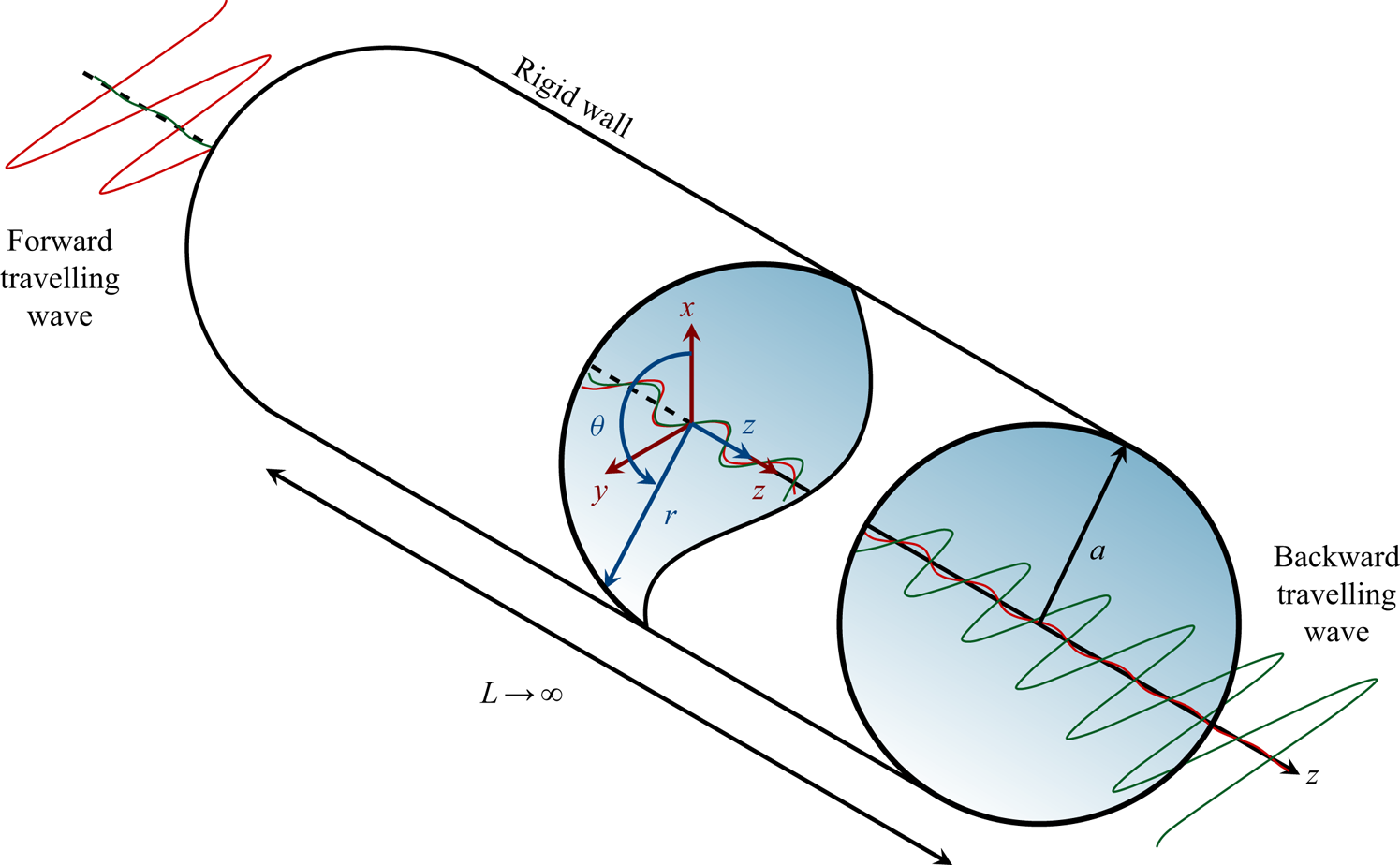
Figure 1. The geometry in a cylindrical coordinate system ( $r, \theta , z$) that serves as a basis for the analytical solution. The fluid is bounded within a rigid tube of radius $a$ and of infinite length $L$.
$L$.
By applying a regular perturbation technique (Hamilton & Blackstock Reference Hamilton and Blackstock1998, p. 281), the problem can be solved in successive steps of increasing order in terms of the small Mach number
 \begin{equation} \varepsilon = \frac{v_{{a}}}{c_{{f}}} \ll 1 , \end{equation}
with the amplitude of the fluid velocity denoted by  $v_{{a}}$, and the speed of sound in the fluid by $c_{{f}}$. The perturbed variables can then be written in the form of a series, namely $\square = \widehat {\square }_0 + \varepsilon \widehat {\square }_1 + \varepsilon ^2 \widehat {\square }_2 + \cdots$, where the subscript denotes the order in the perturbation expansion. In our formulation, we will use $\square _0 = \widehat {\square }_0$, $\square _1 = \varepsilon \widehat {\square }_1$, $\square _2 = \varepsilon ^2 \widehat {\square }_2$, and solve the associated first- and second-order problems. Following our assumptions, $\boldsymbol {v}_0 = \boldsymbol {0}$.
3. Fluid motion at the first order
The perturbation expansion of the governing equations to the first order results in the momentum equations
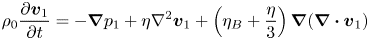 \begin{equation} \rho_0 \frac{\partial \boldsymbol{v}_1}{\partial t} = - \boldsymbol{\nabla} p_1 + \eta \nabla^2 \boldsymbol{v}_1 + \left( \eta_{{B}} + \frac{\eta}{3} \right) \boldsymbol{\nabla} ( \boldsymbol{\nabla} \boldsymbol{\cdot} \boldsymbol{v}_1 ) \end{equation}
and the continuity equation
 \begin{equation} \frac{\partial \rho_1}{\partial t} = - \rho_0 \boldsymbol{\nabla} \boldsymbol{\cdot} \boldsymbol{v}_1 , \end{equation}
with equilibrium density  $\rho _0$. The first-order pressure and density are related through the linear equation of state
 \begin{equation} p_1 = c_{{f}}^2 \rho_1 . \end{equation}
Using the Helmholtz decomposition
 \begin{equation} \boldsymbol{v}_1 = \boldsymbol{\nabla} \varphi_1 + \boldsymbol{\nabla} \times \boldsymbol{\psi}_1 \end{equation}
(e.g. Blackstock Reference Blackstock2001, p. 76), the first-order velocity field can be separated into a sum of the gradient of a scalar velocity potential  $\varphi _1$ and the curl of a divergence-free vector velocity potential $\boldsymbol {\psi }_1$. First-order fields are assumed to have a harmonic time-dependence, i.e. $\square _1 (\boldsymbol {x}, t ) = \mathrm {Re} [ \tilde {\square }_1 ( \boldsymbol {x} ) \textrm {e}^{- \mathrm {i} \omega t} ]$ with angular frequency $\omega$, where $\mathrm {Re} [\square ]$ denotes the real part of $\square$, and $\tilde {\square }_1 ( \boldsymbol {x} )$ is the complex amplitude of the corresponding first-order field $\square _1 (\boldsymbol {x}, t )$. Using this assumption and inserting (3.4) in (3.1), (3.2), (3.3) leads to the set of first-order potential equations
 \begin{gather} \nabla^2 \varphi_1 + k_{{f}}^2 \varphi_1 = 0 , \end{gather}
 \begin{gather}\nabla^2 \boldsymbol{\psi}_1 + k_{{v}}^2 \boldsymbol{\psi}_1 = \boldsymbol{0} , \end{gather}
with the wavenumber in an unbounded viscous fluid
 \begin{equation} k_{{f}} = \frac{\omega}{c_{{f}}} \left[ 1 - \frac{\mathrm{i} \omega}{\rho_0 c_{{f}}^2} \left( \eta_{{B}} + \frac{4}{3} \eta \right) \right]^{- 1/2} \end{equation}
(Blackstock Reference Blackstock2001, p. 305), and the viscous wavenumber
 \begin{equation} k_{{v}} = \frac{\mathrm{i} + 1}{\delta} , \end{equation}
where  $\delta$ represents the thickness of the viscous boundary layer and is computed as
 \begin{equation} \delta = \sqrt{\frac{2 \eta}{\rho_0 \omega}}. \end{equation}
 We assume that there is a forward and a backward travelling wave inside the fluid, which form a pseudo-standing wave along the  $z$-axis when superimposed. The pseudo-standing wave potentials therefore follow as a sum of potentials of forward and backward travelling waves, namely
 \begin{gather} \varphi_1 = \varphi_1^{+} + \varphi_1^{-} , \end{gather}
 \begin{gather}\boldsymbol{\psi}_1 = \boldsymbol{\psi}_1^{+} + \boldsymbol{\psi}_1^{-} , \end{gather}
with superscripts  $\square ^{+}$ and $\square ^{-}$ identifying the forward and the backward travelling waves, respectively. Based on the axial symmetry of the problem, we assume the following form of potentials:
 \begin{gather} \varphi_1^{+} = F (r) \exp({\mathrm{i} ( k z - \omega t )}) , \end{gather}
 \begin{gather}\varphi_1^{-} = F (r) \exp({\mathrm{i} ( - k z - \omega t )}) , \end{gather}
 \begin{gather}\boldsymbol{\psi}_1^{+} = G (r) \exp({\mathrm{i} ( k z - \omega t )}) \boldsymbol{e}_{\theta} , \end{gather}
 \begin{gather}\boldsymbol{\psi}_1^{-} = G (r) \exp({\mathrm{i} ( - k z - \omega t )}) \left( - \boldsymbol{e}_{\theta} \right) , \end{gather}
with the basis vector  $\boldsymbol {e}_{\theta }$ of unit length, unknown functions $F(r)$ and $G(r)$, and an unknown complex wavenumber $k$.
$k$.
To find the functions  $F(r)$ and $G(r)$, we insert the potentials of the forward travelling wave, (3.12) and (3.14), into (3.5) and (3.6), which leads to
 \begin{equation} \left[ \frac{\mathrm{d}^2 F(r)}{\mathrm{d} r^2} + \frac{1}{r} \frac{\mathrm{d} F(r)}{\mathrm{d} r} + q_{{f}}^2 F(r) \right] \exp({\mathrm{i} ( k z - \omega t )}) = 0 \end{equation}
and
 \begin{equation} \left[ \frac{\mathrm{d}^2 G(r)}{\mathrm{d} r^2} + \frac{1}{r} \frac{\mathrm{d} G(r)}{\mathrm{d} r} + \left( q_{{v}}^2 - \frac{1}{r^2} \right) G(r) \right] \exp({\mathrm{i} ( k z - \omega t )}) = 0 , \end{equation}
with
 \begin{gather} q_{{f}}^2 = k_{{f}}^2 - k^2 , \end{gather}
 \begin{gather}q_{{v}}^2 = k_{{v}}^2 - k^2 . \end{gather}
The unknown functions  $F(r)$ and $G(r)$ are the solutions to the Sturm–Liouville equations that follow from the $r$-dependent part of (3.16) and (3.17), and can be expressed as
 \begin{gather} F ( r ) = A_1 J_0 (q_{{f}} r) + A_2 Y_0 (q_{{f}} r) , \end{gather}
 \begin{gather}G ( r ) = B_1 J_1 (q_{{v}} r) + B_2 Y_1 (q_{{v}} r) , \end{gather}
with constants  $A_1$, $A_2$, $B_1$, $B_2$, and $n$th-order Bessel functions $J_n$ and $Y_n$ of the first and of the second kind, respectively. Because the velocity has to be finite at $r = 0$, $A_2$ and $B_2$ have to be zero, which yields
 \begin{gather} F ( r ) = A_1 J_0 (q_{{f}} r) , \end{gather}
 \begin{gather}G ( r ) = B_1 J_1 (q_{{v}} r) . \end{gather}
3.1. Dispersion relation and the unknown constants at the first order
The first-order velocity field of a forward travelling wave can be written in a potential form as
 \begin{equation} \boldsymbol{v}_1^{+} = \boldsymbol{\nabla} \varphi_1^{+} + \boldsymbol{\nabla} \times \boldsymbol{\psi}_1^{+} . \end{equation}
We substitute (3.12) and (3.14) into (3.24), which leads to the velocity field of a forward travelling wave,
 \begin{align} \boldsymbol{v}_1^{+} = \left[ \left( \frac{\mathrm{d} F(r)}{\mathrm{d}r} - \mathrm{i} k G(r) \right) \boldsymbol{e}_r + \left( \mathrm{i} k F(r) + \frac{1}{r} G(r) + \frac{\mathrm{d} G(r)}{\mathrm{d}r} \right) \boldsymbol{e}_z \right] \exp({\mathrm{i} (kz - \omega t)}) , \end{align}
with basis vectors  $\boldsymbol {e}_r$ and $\boldsymbol {e}_z$ of the cylindrical coordinate system. In order to find the dispersion relation and the unknown constants $A_1$ and $B_1$, we apply the no-slip boundary condition to the fluid at the wall of the tube, namely
 \begin{equation} \left.\boldsymbol{v}_1^{+} \right|_{r=a} = \boldsymbol{0} , \end{equation}
where  $\square |_{r=a}$ denotes the evaluation of $\square$ at $r=a$. Substituting the solutions (3.22) and (3.23) into (3.25) and using the condition (3.26) leads to a system of two equations,
 \begin{gather} \left[ - q_{{f}} J_1 (q_{{f}} a) \right] A_1 + \left[ -\mathrm{i} k J_1 (q_{{v}} a) \right] B_1 = 0 , \end{gather}
 \begin{gather} \left[ \mathrm{i} k J_0 (q_{{f}} a) \right] A_1 + \left[ q_{{v}} J_0 (q_{{v}} a) \right] B_1 = 0 . \end{gather}
The system of (3.27) and (3.28) has a non-trivial solution only if the determinant of the system equals zero, i.e.
 \begin{equation} \left| \begin{array}{@{}cc@{}} - q_{{f}} J_1 (q_{{f}} a) & -\mathrm{i} k J_1 (q_{{v}} a) \\ \mathrm{i} k J_0 (q_{{f}} a) & q_{{v}} J_0 (q_{{v}} a)\end{array}\right| = 0 . \end{equation}
This leads to the dispersion relation
 \begin{equation} K ( k_{{R}}, k_{{I}}) = q_{{f}} q_{{v}} J_0 ( q_{{v}} a ) J_1 ( q_{{f}} a ) + k^2 J_0 ( q_{{f}} a ) J_1 ( q_{{v}} a ) = 0 , \end{equation}
which is used to numerically find the real and the imaginary parts of the wavenumber  $k$, defined as $k_{{R}} = \mathrm {Re} [k]$ and $k_{{I}} = \mathrm {Im} [k]$, respectively. The equations leading to both parts of the wavenumber are
 \begin{gather} \mathrm{Re} \left[ K ( k_{{R}} , k_{{I}} ) \right] = 0 , \end{gather}
 \begin{gather}\mathrm{Im} \left[ K ( k_{{R}}, k_{{I}}) \right] = 0 . \end{gather}
The wavenumber is later calculated for water, oil, glycerol and air (see § 5 and appendix A).
We can now use one of the equations, e.g. (3.27), and express one of the unknown constants in terms of the second, which is a fitting parameter determined by the pressure profile of the wave. In our case, we choose  $A_1$ as a fitting parameter, and $B_1$ then follows as
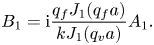 \begin{equation} B_1 = \mathrm{i} \frac{q_{{f}} J_1 (q_{{f}} a)}{k J_1 (q_{{v}} a)} A_1 . \end{equation}
3.2. First-order velocity field
The velocity field of the backward travelling wave is obtained by substituting (3.13) and (3.15) into (3.4):
 \begin{equation} \boldsymbol{v}_1^{-} = \left[ \left( \frac{\mathrm{d} F(r)}{\mathrm{d}r} - \mathrm{i} k G(r) \right) \boldsymbol{e}_r + \left( - \mathrm{i} k F(r) - \frac{1}{r} G(r) - \frac{\mathrm{d} G(r)}{\mathrm{d}r} \right) \boldsymbol{e}_z \right] \exp({\mathrm{i} ( - kz - \omega t)}) . \end{equation}
The total velocity field is then obtained by summing (3.25) and (3.34):
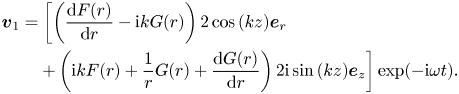 \begin{align} \boldsymbol{v}_1 &= \left[ \left( \frac{\mathrm{d} F (r)}{\mathrm{d} r} - \mathrm{i} k G(r) \right) 2 \cos{(k z)} \boldsymbol{e}_r \right. \nonumber\\ &\quad \left. + \left( \mathrm{i} k F(r) + \frac{1}{r} G (r) + \frac{\mathrm{d} G (r)}{\mathrm{d} r} \right) 2 \mathrm{i} \sin{(k z)} \boldsymbol{e}_z \right] \exp({- \mathrm{i} \omega t}) . \end{align}
Substituting the solutions (3.22) and (3.23) for  $F(r)$ and $G(r)$, respectively, into (3.35) yields the total first-order velocity:
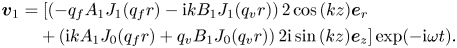 \begin{align} \boldsymbol{v}_1 &= \left[ \left( - q_{{f}} A_1 J_1 (q_{{f}} r) - \mathrm{i} k B_1 J_1 (q_{{v}} r) \right) 2 \cos{(k z)} \boldsymbol{e}_r \right. \nonumber\\ &\quad \left. + \left( \mathrm{i} k A_1 J_0 (q_{{f}} r) + q_{{v}} B_1 J_0 (q_{{v}} r) \right) 2 \mathrm{i} \sin{(k z)} \boldsymbol{e}_z \right] \exp({- \mathrm{i} \omega t}) . \end{align}
3.3. Constants in terms of the pressure amplitude
For easier physical interpretation of the constants  $A_1$ and $B_1$, we express them here in terms of the pressure amplitude $p_{{a}}$ at $z = 0$. Using the equation of state (3.3) in combination with the continuity equation (3.2) leads to the following relation:
 \begin{equation} p_1 = - \frac{\mathrm{i} \rho_0 c_{{f}}^2}{\omega} \boldsymbol{\nabla} \boldsymbol{\cdot} \boldsymbol{v}_1 . \end{equation}
Applying the solution for the first-order velocity (3.36) to the pressure–velocity relation (3.37) yields the pressure field
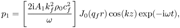 \begin{equation} p_1 = \left[ \frac{2 \mathrm{i} A_1 k_{{f}}^2 \rho_0 c_{{f}}^2}{\omega} \right] J_0 (q_{{f}} r) \cos (k z) \exp({- \mathrm{i} \omega t}) , \end{equation}
where the fraction inside the brackets is the amplitude of the pressure field  $p_1$; that is,
 \begin{equation} p_{{a}} = \frac{2 \mathrm{i} A_1 k_{{f}}^2 \rho_0 c_{{f}}^2}{\omega} . \end{equation}
Now, the constant  $A_1$ can be expressed directly from (3.39) as
 \begin{equation} A_1 = - \frac{\mathrm{i} p_{{a}} \omega}{2 k_{{f}}^2 \rho_0 c_{{f}}^2} . \end{equation}
The remaining constant follows from combining (3.40) and (3.33):
 \begin{equation} B_1 = \frac{p_{{a}} \omega q_{{f}}}{2 k_{{f}}^2 \rho_0 c_{{f}}^2 k} \frac{J_1 (q_{{f}} a)}{J_1 (q_{{v}} a)} . \end{equation}
 Even though we consider only the lowest mode of propagation, the wave is not plane, but, as evident in (3.38), contains  $r$-dependency due to the wave attenuation in the viscous boundary layer. A similar result was also obtained by Qi et al. (Reference Qi, Johnson and Harris1995), but their study is restricted to wide channels ( $a\gg \delta$).
4. Steady fluid motion at the second order
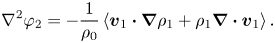
The steady second-order equations are obtained by time-averaging the equations that follow from the second-order perturbation expansion. The set of the so-called streaming equations comprises the continuity equation
 \begin{equation} \boldsymbol{\nabla} \boldsymbol{\cdot} \left\langle \boldsymbol{v}_2 \right\rangle = - \frac{1}{\rho_0} \boldsymbol{\nabla} \boldsymbol{\cdot} \left\langle \rho_1 \boldsymbol{v}_1 \right\rangle \end{equation}
and the momentum equations
 \begin{equation} \boldsymbol{\nabla} \left\langle p_2 \right\rangle - \eta \nabla^2 \left\langle \boldsymbol{v}_2 \right\rangle - \left( \eta_{{B}} + \frac{\eta}{3} \right) \boldsymbol{\nabla} \left( \boldsymbol{\nabla} \boldsymbol{\cdot} \left\langle \boldsymbol{v}_2 \right\rangle \right)= - \rho_0 \boldsymbol{\nabla} \boldsymbol{\cdot} \left\langle \boldsymbol{v}_1 \boldsymbol{v}_1 \right\rangle , \end{equation}
where the body force on the right-hand side is the spatial variation of the Reynolds stress (Lighthill Reference Lighthill1978). The time-average is denoted by
 \begin{equation} \left\langle \square \right\rangle = \frac{1}{T} \int_{0}^{T} \square \, \mathrm{d} t , \end{equation}
with the first-order oscillation period  $T$.
$T$.
The streaming velocity can be decomposed as
 \begin{equation} \left\langle \boldsymbol{v}_2 \right\rangle = \boldsymbol{\nabla} \varphi_2 +\boldsymbol{\nabla} \times \boldsymbol{\varPsi}_2 , \end{equation}
where  $\varphi _2$ is the scalar velocity potential and $\boldsymbol {\varPsi }_2$ is the divergence-free vector potential. Substituting (4.4) in (4.2) and applying the curl to the resulting equation leads to
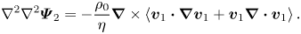 \begin{equation} \nabla^2 \nabla^2 \boldsymbol{\varPsi}_2 = - \frac{\rho_0}{\eta} \boldsymbol{\nabla} \times \left\langle \boldsymbol{v}_1 \boldsymbol{\cdot} \boldsymbol{\nabla} \boldsymbol{v}_1 + \boldsymbol{v}_1 \boldsymbol{\nabla} \boldsymbol{\cdot} \boldsymbol{v}_1 \right\rangle . \end{equation}
In the process of simplifying the terms on the right-hand side of (4.5), we will use the first-order velocity field (3.35) and the following identities:
 \begin{gather} \sin (k^{*} z) \cos (k z) = \tfrac{1}{2} [ \sin (2 k_{{R}} z) - \mathrm{i} \sinh (2 k_{{I}} z)] , \end{gather}
 \begin{gather}\sin (k z) \cos (k^{*} z) = \tfrac{1}{2} [ \sin (2 k_{{R}} z) + \mathrm{i} \sinh (2 k_{{I}} z)] , \end{gather}
where  $k_{{R}}$ and $k_{{I}}$ are respectively the real and imaginary part of the wavenumber, and $\square ^{*}$ denotes the complex conjugate of $\square$. Equation (4.5) can now be reformulated into
 \begin{equation} \nabla^2 \nabla^2 \boldsymbol{\varPsi}_2 = - \frac{\rho_0}{\eta} \mathrm{Re} \left\{ \sin (2 k_{{R}} z) \left[ R_{{R}} (r) + E_{{R}} (r) \right] + \mathrm{i} \sinh (2 k_{{I}} z) \left[ R_{{I}} (r) + E_{{I}} (r) \right] \right\} \boldsymbol{e}_{\theta} , \end{equation}
with the functions  $R_{{R}} (r)$, $R_{{I}} (r)$ resulting from the first term in the angle brackets on the right-hand side of (4.5), and the functions $E_{{R}} (r)$, $E_{{I}} (r)$ originating from the second term. We use separate functions for easier analysis of the individual contributions at a later stage, because the dropping of the second term in the angle brackets on the right-hand side of (4.5) is a very common assumption (e.g. Rayleigh Reference Rayleigh1884; Schlichting Reference Schlichting1932; Lighthill Reference Lighthill1978; Doinikov et al. Reference Doinikov, Thibault and Marmottant2017). The four functions are given explicitly in appendix C.
The geometry of the problem suggests
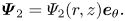 \begin{equation} \boldsymbol{\varPsi}_2 = \varPsi_2 (r, z) \boldsymbol{e}_{\theta}. \end{equation}
Substituting (4.9) into (4.8) and eliminating the basis vector yields the following expression:
 \begin{equation} \varDelta_{\theta}^2 \varPsi_2 = - \frac{\rho_0}{\eta} \mathrm{Re} \left\{ \sin (2 k_{{R}} z) \left[ R_{{R}} (r) + E_{{R}} (r) \right] + \mathrm{i} \sinh (2 k_{{I}} z) \left[ R_{{I}} (r) + E_{{I}} (r) \right] \right\} , \end{equation}
where we applied the operator  $\varDelta _{\theta }$, defined as
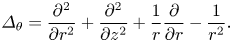 \begin{equation} \varDelta_{\theta} = \frac{\partial^2}{\partial r^2} + \frac{\partial^2}{\partial z^2} + \frac{1}{r} \frac{\partial}{\partial r} - \frac{1}{r^2} . \end{equation}
Based on the right-hand side of (4.10), we assume
 \begin{equation} \varPsi_2 (r, z) = - \frac{\rho_0}{\eta} \mathrm{Re} \left\{ \sin (2 k_{{R}} z) S_{{R}} (r) + \mathrm{i} \sinh (2 k_{{I}} z) S_{{I}} (r) \right\}, \end{equation}
with the unknown functions  $S_{{R}} (r)$ and $S_{{I}} (r)$. Substituting (4.12) into (4.10) gives two ordinary fourth-order differential equations,
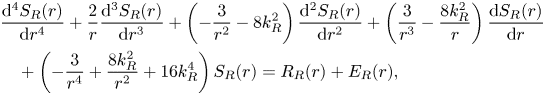 \begin{align} &\frac{\mathrm{d}^4 S_{{R}}(r)}{\mathrm{d} r^4} + \frac{2}{r} \frac{\mathrm{d}^3 S_{{R}}(r)}{\mathrm{d} r^3} + \left( - \frac{3}{r^2} - 8 k_{{R}}^2 \right) \frac{\mathrm{d}^2 S_{{R}}(r)}{\mathrm{d} r^2} + \left( \frac{3}{r^3} - \frac{8 k_{{R}}^2}{r} \right) \frac{\mathrm{d} S_{{R}}(r)}{\mathrm{d} r}\nonumber\\ &\quad + \left( - \frac{3}{r^4} + \frac{8 k_{{R}}^2}{r^2} + 16 k_{{R}}^4 \right) S_{{R}}(r) = R_{{R}}(r) + E_{{R}}(r),\end{align}
 \begin{align} &\frac{\mathrm{d}^4 S_{{I}}(r)}{\mathrm{d} r^4} + \frac{2}{r} \frac{\mathrm{d}^3 S_{{I}}(r)}{\mathrm{d} r^3} + \left( - \frac{3}{r^2} + 8 k_{{I}}^2 \right) \frac{\mathrm{d}^2 S_{{I}}(r)}{\mathrm{d} r^2} + \left( \frac{3}{r^3} + \frac{8 k_{{I}}^2}{r} \right) \frac{\mathrm{d} S_{{I}}(r)}{\mathrm{d} r} \nonumber\\ &\quad +\left( - \frac{3}{r^4} - \frac{8 k_{{I}}^2}{r^2} + 16 k_{{I}}^4 \right) S_{{I}}(r) = R_{{I}}(r) + E_{{I}}(r) , \end{align}
which we must solve in order to find the stream function  $\varPsi _2 (r, z)$. In the process, it will be convenient to define the linear differential operator
 \begin{equation} \varDelta_1 = \frac{\mathrm{d}^2 }{\mathrm{d} r^2} + \frac{1}{r} \frac{\mathrm{d}}{\mathrm{d} r} - \frac{1}{r^2} \end{equation}
and use it to transform (4.13) and (4.14) into
 \begin{equation} \varDelta_1 \varDelta_1 S_{{R}}(r) - 8 k_{{R}}^2 \varDelta_1 S_{{R}}(r) + 16 k_{{R}}^4 S_{{R}}(r) = R_{{R}}(r) + E_{{R}}(r) \end{equation}
and
 \begin{equation} \varDelta_1 \varDelta_1 S_{{I}}(r) + 8 k_{{I}}^2 \varDelta_1 S_{{I}}(r) + 16 k_{{I}}^4 S_{{I}}(r) = R_{{I}}(r) + E_{{I}}(r) , \end{equation}
respectively.
To solve (4.16) and (4.17), we will make use of the linear finite Hankel transform of order one (introduced by Sneddon Reference Sneddon1946, Reference Sneddon1972), which is defined as
 \begin{equation} \mathcal{H}_1 \{ f (r) \} = \int_0^b r f (r) J_1 ( \xi_i r )\,\textrm{d}r = \bar{f} (\xi_{i}) \end{equation}
for a function  $f(r)$ integrable on the interval $0 \leqslant r \leqslant b$. The corresponding inverse transform follows as
 \begin{equation} \mathcal{H}_1^{-1} \left\{ \bar{f} (\xi_{i}) \right\} = f (r) = \frac{2}{b^2} \sum_{i=1}^{\infty} \bar{f} (\xi_{i}) \frac{J_1 ( \xi_i r )}{\left[J_2 ( \xi_i b )\right]^2} , \end{equation}
with  $\bar {\square }$ denoting the transformed expression, and provided that $\xi _i$ with $i=1,2,3,\ldots$ are the positive roots of the transcendental equation
 \begin{equation} J_1 ( \xi_i b ) = 0 . \end{equation}
The transformation of  $\varDelta _1$ that is applied to a function $f(r)$ gives (Sneddon Reference Sneddon1946, Reference Sneddon1972)
 \begin{equation} \mathcal{H}_1 \left\{ \varDelta_1 f (r) \right\} = - \xi_i^2 \bar{f} (\xi_i) + b \xi_i f (b) J_2 ( \xi_i b ) . \end{equation}
 Applying the finite Hankel transform defined in (4.18) to the differential (4.16), limiting the domain of transformation with the radius of the tube  $a$, and exploiting the property specified in (4.21) yields
 \begin{gather} \xi_i^4 \bar{S}_{{R}}(\xi_{i}) - a \xi_i^3 S_{{R}}(r) \big|_{r=a} J_2 (\xi_i a) + 8 k_{{R}}^2 \xi_i^2 \bar{S}_{{R}}(\xi_{i}) + a \xi_i \varDelta_1 S_{{R}}(r) \big|_{r=a} J_2 (\xi_i a) \nonumber\\ + 8 k_{{R}}^2 a \xi_i S_{{R}}(r) \big|_{r=a} + 16 k_{{R}}^4 \bar{S}_{{R}}(\xi_{i}) = \bar{R}_{{R}}(\xi_{i}) + \bar{E}_{{R}}(\xi_{i}) . \end{gather}
The transformed unknown function  $\bar {S}_{{R}}(\xi _{i})$ can be expressed from (4.22) as
 \begin{align} \bar{S}_{{R}}(\xi_{i}) = \frac{1}{( \xi_i^2 + 4 k_{{R}}^2)^2} [\bar{R}_{{R}}(\xi_{i}) + \bar{E}_{{R}}(\xi_{i}) - a \xi_i C_1 J_2 ( \xi_i a ) + a \xi_i C_2 ( \xi_i^2 J_2 ( \xi_i a ) - 8 k_{{R}}^2) ] , \end{align}
with the constants  $C_1$ and $C_2$ defined as
 \begin{gather} C_1 = \varDelta_1 S_{{R}}(r) \big|_{r=a} , \end{gather}
 \begin{gather}C_2 = S_{{R}}(r) \big|_{r=a} . \end{gather}
The function  $S_{{R}}(r)$ can be obtained by applying the inverse transform (4.19)–(4.23), i.e.
 \begin{align} S_{{R}}(r) &= \frac{2}{a^2} \sum_{i=1}^{\infty} \frac{J_1 ( \xi_i r )}{[J_2 ( \xi_i a )]^2 (\xi_i^2 + 4 k_{{R}}^2 )^2} [ \bar{R}_{{R}}(\xi_{i}) + \bar{E}_{{R}}(\xi_{i}) \nonumber\\ &\quad - a \xi_i C_1 J_2 ( \xi_i a ) + a \xi_i C_2 ( \xi_i^2 J_2 ( \xi_i a ) - 8 k_{{R}}^2) ]. \end{align}
The second unknown function,  $S_{{I}}(r)$, can be obtained by applying an analogous procedure to the differential equation (4.17). The resulting expression can be written as
 \begin{align} S_{{I}}(r) &= \frac{2}{a^2} \sum_{i=1}^{\infty} \frac{J_1 ( \xi_i r )}{[J_2 ( \xi_i a )]^2 ( \xi_i^2 - 4 k_{{I}}^2 )^2} [\bar{R}_{{I}}(\xi_{i}) + \bar{E}_{{I}}(\xi_{i})\nonumber\\ &\quad - a \xi_i C_3 J_2 ( \xi_i a ) + a \xi_i C_4 ( \xi_i^2 J_2 ( \xi_i a ) + 8 k_{{I}}^2)] , \end{align}
where the constants are defined as
 \begin{gather} C_3 = \varDelta_1 S_{{I}}(r) \big|_{r=a} , \end{gather}
 \begin{gather}C_4 = S_{{I}}(r) \big|_{r=a} . \end{gather}
Returning to the decomposition of the streaming velocity (4.4) and substituting it into (4.1) leads to
 \begin{equation} \nabla^2 \varphi_2 = - \frac{1}{\rho_0} \left\langle \boldsymbol{v}_1 \boldsymbol{\cdot} \boldsymbol{\nabla} \rho_1 + \rho_1 \boldsymbol{\nabla} \boldsymbol{\cdot} \boldsymbol{v}_1 \right\rangle. \end{equation}
Using the first-order velocity field (3.35), the first-order pressure field (3.38), the equation of state (3.3) and the identities
 \begin{gather} \cos (k^{*} z) \cos (k z) = \tfrac{1}{2} [ \cos (2 k_{{R}} z) + \cosh (2 k_{{I}} z)] , \end{gather}
 \begin{gather}\sin (k^{*} z) \sin (k z) = \tfrac{1}{2} [ -\cos (2 k_{{R}} z) + \cosh (2 k_{{I}} z)] \end{gather}
transforms (4.30) into
 \begin{equation} \nabla^2 \varphi_2 = - \frac{p_{{a}}}{2 \rho_0 c_{{f}}} \mathrm{Re} \left\{ \cos (2 k_{{R}} z) M_{{R}} (r) + \cosh (2 k_{{I}} z) M_{{I}} (r) \right\} , \end{equation}
with the source terms  $M_{{R}} (r)$ and $M_{{I}} (r)$ given in appendix D. We assume, based on (4.33), that the solution has the following form:
 \begin{equation} \varphi_2 (r,z) = - \frac{p_{{a}}}{2 \rho_0 c_{{f}}} \mathrm{Re} \left\{ \cos (2 k_{{R}} z) U_{{R}} (r) + \cosh (2 k_{{I}} z) U_{{I}} (r) \right\} . \end{equation}
The unknown functions  $U_{{R}} (r)$ and $U_{{I}} (r)$ can be obtained by solving two differential equations that follow from substituting (4.34) into (4.33), namely
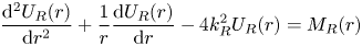 \begin{equation} \frac{\mathrm{d}^2 U_{{R}} (r) }{\mathrm{d} r^2} + \frac{1}{r} \frac{\mathrm{d} U_{{R}} (r) }{\mathrm{d} r} - 4 k_{{R}}^2 U_{{R}} (r) = M_{{R}} (r) \end{equation}
and
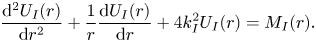 \begin{equation} \frac{\mathrm{d}^2 U_{{I}} (r) }{\mathrm{d} r^2} + \frac{1}{r} \frac{\mathrm{d} U_{{I}} (r) }{\mathrm{d} r} + 4 k_{{I}}^2 U_{{I}} (r) = M_{{I}} (r) . \end{equation}
The general solutions to the homogeneous equations related to (4.35) and (4.36), denoted by the superscript  $\square ^{{H}}$, follow as
 \begin{equation} U_{{R}}^{{H}} (r) = C_5 J_0 (2 \mathrm{i} k_{{R}} r) + C_6 Y_0 (-2 \mathrm{i} k_{{R}} r) \end{equation}
and
 \begin{equation} U_{{I}}^{{H}} (r) = C_7 J_0 (2 k_{{I}} r) + C_8 Y_0 (2 k_{{I}} r) , \end{equation}
respectively, with the unknown constants  $C_5$, $C_6$, $C_7$, $C_8$. The particular solutions to (4.35) and (4.36), denoted by the superscript $\square ^{{P}}$, are obtained by the method of variation of parameters (e.g. Boyce, DiPrima & Meade Reference Boyce, DiPrima and Meade2017), and follow as
 \begin{align} U_{{R}}^{{P}} (r) &= - \frac{\rm \pi}{2} J_0 (2 \mathrm{i} k_{{R}} r) \int_0^r x M_{{R}} (x) Y_0 (-2 \mathrm{i} k_{{R}} x) \, \mathrm{d}x \nonumber\\ &\quad + \frac{\rm \pi}{2} Y_0 (-2 \mathrm{i} k_{{R}} r) \int_0^r x M_{{R}} (x) J_0 (2 \mathrm{i} k_{{R}} x) \, \mathrm{d}x \end{align}
and
 \begin{align} U_{{I}}^{{P}} (r) = - \frac{\rm \pi}{2} J_0 (2 k_{{I}} r) \int_0^r x M_{{I}} (x) Y_0 (2 k_{{I}} x) \, \mathrm{d}x + \frac{\rm \pi}{2} Y_0 (2 k_{{I}} r) \int_0^r x M_{{I}} (x) J_0 (2 k_{{I}} x) \, \mathrm{d}x, \end{align}
respectively. The general solutions to (4.35) and (4.36) are sums of solutions to the related homogeneous equations,  $U_{{R}}^{{H}} (r)$ and $U_{{I}}^{{H}} (r)$, and of particular solutions, $U_{{R}}^{{P}} (r)$ and $U_{{I}}^{{P}} (r)$. Therefore, the general solutions are given as
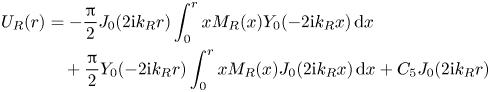 \begin{align} U_{{R}} (r) &= - \frac{\rm \pi}{2} J_0 (2 \mathrm{i} k_{{R}} r) \int_0^r x M_{{R}} (x) Y_0 (-2 \mathrm{i} k_{{R}} x) \, \mathrm{d}x \nonumber\\ &\quad + \frac{\rm \pi}{2} Y_0 (-2 \mathrm{i} k_{{R}} r) \int_0^r x M_{{R}} (x) J_0 (2 \mathrm{i} k_{{R}} x) \, \mathrm{d}x + C_5 J_0 (2 \mathrm{i} k_{{R}} r) \end{align}
and
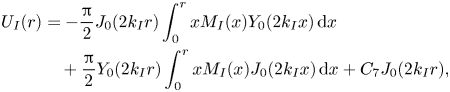 \begin{align} U_{{I}} (r) &= - \frac{\rm \pi}{2} J_0 (2 k_{{I}} r) \int_0^r x M_{{I}} (x) Y_0 (2 k_{{I}} x) \, \mathrm{d}x \nonumber\\ &\quad + \frac{\rm \pi}{2} Y_0 (2 k_{{I}} r) \int_0^r x M_{{I}} (x) J_0 (2 k_{{I}} x) \, \mathrm{d}x + C_7 J_0 (2 k_{{I}} r), \end{align}
where we applied  $C_6 = 0$ and $C_8=0$, since the solution has to remain finite at $r = 0$.
4.1. Streaming velocity
The streaming velocity  $\left \langle \boldsymbol {v}_2 \right \rangle$ from (4.4) can be expressed in terms of the functions $S_{{R}}(r)$, $S_{{I}}(r)$, $U_{{R}}(r)$ and $U_{{I}}(r)$ as
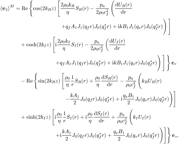
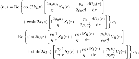 \begin{align} \left\langle \boldsymbol{v}_2 \right\rangle &= \mathrm{Re} \left\{ \cos (2 k_{{R}} z) \left[ \frac{2 \rho_0 k_{{R}}}{\eta} S_{{R}}(r) - \frac{p_{{a}}}{2 \rho_0 c_{{f}}^2} \frac{\mathrm{d} U_{{R}} (r)}{\mathrm{d} r} \right]\right. \nonumber\\ &\qquad\quad \left.+ \cosh (2 k_{{I}} z) \left[ \mathrm{i} \frac{2 \rho_0 k_{{I}}}{\eta} S_{{I}}(r) - \frac{p_{{a}}}{2 \rho_0 c_{{f}}^2} \frac{\mathrm{d} U_{{I}} (r)}{\mathrm{d} r} \right] \right\} \boldsymbol{e}_r \nonumber\\&\quad - \mathrm{Re} \left\{ \sin (2 k_{{R}} z) \left[ \frac{\rho_0}{\eta} \frac{1}{r} S_{{R}}(r) + \frac{\rho_0}{\eta} \frac{\mathrm{d} S_{{R}}(r)}{\mathrm{d} r} - \frac{p_{{a}} k_{{R}}}{\rho_0 c_{{f}}^2} U_{{R}}(r) \right]\right. \nonumber\\ &\qquad\qquad \left.+ \sinh (2 k_{{I}} z) \left[ \mathrm{i} \frac{\rho_0}{\eta} \frac{1}{r} S_{{I}}(r) + \mathrm{i} \frac{\rho_0}{\eta} \frac{\mathrm{d} S_{{I}}(r)}{\mathrm{d} r} + \frac{p_{{a}} k_{{I}}}{\rho_0 c_{{f}}^2} U_{{I}}(r) \right] \right\} \boldsymbol{e}_z , \end{align}
where the derivatives  $\mathrm {d} S_{{R}}(r) / \mathrm {d} r$, $\mathrm {d} S_{{I}}(r) / \mathrm {d} r$, $\mathrm {d} U_{{R}}(r) / \mathrm {d} r$, $\mathrm {d} U_{{I}}(r) / \mathrm {d} r$ follow from (4.26), (4.27), (4.41), (4.42), respectively, and are given in appendix E.
The expression (4.43) is a time-averaged Eulerian streaming velocity, which has often been the final result of classical studies (e.g. Rayleigh Reference Rayleigh1884; Schlichting Reference Schlichting1932; Schuster & Matz Reference Schuster and Matz1940). However, the observable behaviour of the fluid undergoing streaming, e.g. by particle image velocimetry (Wiklund, Green & Ohlin Reference Wiklund, Green and Ohlin2012), is better represented by the time-averaged Lagrangian velocity (Westervelt Reference Westervelt1953) or by the average mass transport velocity (Nyborg Reference Nyborg1965). The time-averaged Lagrangian velocity is defined as
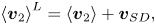 \begin{equation} \left\langle \boldsymbol{v}_2 \right\rangle^{{L}} = \left\langle \boldsymbol{v}_2 \right\rangle + \boldsymbol{v}_{{SD}} , \end{equation}
where  $\boldsymbol {v}_{{SD}}$ is the Stokes drift,
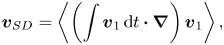 \begin{equation} \boldsymbol{v}_{{SD}} = \left\langle \left( \int \boldsymbol{v}_{1}\,\mathrm{d} t \boldsymbol{\cdot} \boldsymbol{\nabla} \right) \boldsymbol{v}_{1} \right\rangle , \end{equation}
given in appendix F. The average mass transport velocity follows as
 \begin{equation} \left\langle \boldsymbol{v}_2 \right\rangle^{{M}} = \left\langle \boldsymbol{v}_2 \right\rangle + \frac{1}{\rho_0} \left\langle \rho_1 \boldsymbol{v}_1 \right\rangle , \end{equation}
and is divergence-free, which follows from (4.1). Using (3.3), (3.38) and (3.36), together with (4.46), leads to
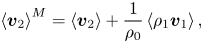
 \begin{align} \left\langle \boldsymbol{v}_2 \right\rangle^{{M}} &= \mathrm{Re} \left\{ \cos (2 k_{{R}} z) \left[ \frac{2 \rho_0 k_{{R}}}{\eta} S_{{R}}(r) - \frac{p_{{a}}}{2 \rho_0 c_{{f}}^2} \left( \frac{\mathrm{d} U_{{R}} (r)}{\mathrm{d} r}\vphantom{\frac{\rho_0}{\eta} \frac{1}{r} S_{{R}}(r) + \frac{\rho_0}{\eta} \frac{\mathrm{d} S_{{R}}(r)}{\mathrm{d} r} - \frac{p_{{a}}}{\rho_0 c_{{f}}^2}}\vphantom{\frac{\rho_0}{\eta} \frac{1}{r} S_{{R}}(r) + \frac{\rho_0}{\eta} \frac{\mathrm{d} S_{{R}}(r)}{\mathrm{d} r} - \frac{p_{{a}}}{\rho_0 c_{{f}}^2}} \right.\right.\right.\nonumber\\ &\hspace{7pc} \left.\left. + q_{{f}} A_1 J_1 (q_{{f}} r) J_0 (q_{{f}}^{*} r) + \mathrm{i} k B_1 J_1 (q_{{v}} r) J_0 (q_{{f}}^{*} r) \vphantom{\frac{p_{{a}}}{2 \rho_0 c_{{f}}^2}}\right) \vphantom{\frac{p_{{a}}}{2 \rho_0 c_{{f}}^2}}\right] \nonumber\\ &\quad + \cosh (2 k_{{I}} z) \left[ \mathrm{i} \frac{2 \rho_0 k_{{I}}}{\eta} S_{{I}}(r) - \frac{p_{{a}}}{2 \rho_0 c_{{f}}^2} \left( \frac{\mathrm{d} U_{{I}} (r)}{\mathrm{d} r} \right.\right.\nonumber\\ &\hspace{6pc} \left.\left.\left.+ q_{{f}} A_1 J_1 (q_{{f}} r) J_0 (q_{{f}}^{*} r) + \mathrm{i} k B_1 J_1 (q_{{v}} r) J_0 (q_{{f}}^{*} r) \vphantom{\frac{p_{{a}}}{2 \rho_0 c_{{f}}^2}}\right) \vphantom{\frac{p_{{a}}}{2 \rho_0 c_{{f}}^2}}\right] \vphantom{\frac{p_{{a}}}{2 \rho_0 c_{{f}}^2}}\right\} \boldsymbol{e}_r \nonumber\\ &\quad - \mathrm{Re} \left\{ \sin (2 k_{{R}} z) \left[ \frac{\rho_0}{\eta} \frac{1}{r} S_{{R}}(r) + \frac{\rho_0}{\eta} \frac{\mathrm{d} S_{{R}}(r)}{\mathrm{d} r} - \frac{p_{{a}}}{\rho_0 c_{{f}}^2} \left( k_{{R}} U_{{R}}(r) \vphantom{\frac{\rho_0}{\eta} \frac{1}{r} S_{{R}}(r) + \frac{\rho_0}{\eta} \frac{\mathrm{d} S_{{R}}(r)}{\mathrm{d} r} - \frac{p_{{a}}}{\rho_0 c_{{f}}^2}}\right.\right.\right.\nonumber\\ &\hspace{7.6pc} \left.\left.- \frac{k A_1}{2} J_0 (q_{{f}} r) J_0 (q_{{f}}^{*} r) + \mathrm{i} \frac{q_{{v}} B_1}{2} J_0 (q_{{v}} r) J_0 (q_{{f}}^{*} r)\vphantom{\frac{\rho_0}{\eta} \frac{1}{r} S_{{R}}(r) + \frac{\rho_0}{\eta} \frac{\mathrm{d} S_{{R}}(r)}{\mathrm{d} r} - \frac{p_{{a}}}{\rho_0 c_{{f}}^2}} \right) \right] \nonumber\\ &\quad + \sinh (2 k_{{I}} z) \left[ \mathrm{i} \frac{\rho_0}{\eta} \frac{1}{r} S_{{I}}(r) + \mathrm{i} \frac{\rho_0}{\eta} \frac{\mathrm{d} S_{{I}}(r)}{\mathrm{d} r} + \frac{p_{{a}}}{\rho_0 c_{{f}}^2} \left( k_{{I}} U_{{I}}(r)\vphantom{\frac{\rho_0}{\eta} \frac{1}{r} S_{{R}}(r) + \frac{\rho_0}{\eta} \frac{\mathrm{d} S_{{R}}(r)}{\mathrm{d} r} - \frac{p_{{a}}}{\rho_0 c_{{f}}^2}} \right.\right.\nonumber\\ &\hspace{6pc} \left.\left.\left. + \mathrm{i} \frac{k A_1}{2} J_0 (q_{{f}} r) J_0 (q_{{f}}^{*} r) + \frac{q_{{v}} B_1}{2} J_0 (q_{{v}} r) J_0 (q_{{f}}^{*} r)\vphantom{\frac{\rho_0}{\eta} \frac{1}{r} S_{{R}}(r) + \frac{\rho_0}{\eta} \frac{\mathrm{d} S_{{R}}(r)}{\mathrm{d} r} - \frac{p_{{a}}}{\rho_0 c_{{f}}^2}} \right) \right] \right\} \boldsymbol{e}_z. \end{align}
4.2. Unknown constants at the second order
To find the constants  $C_1$, $C_2$, $C_3$, $C_4$, $C_5$ and $C_7$ appearing in (4.26), (4.27), (4.41) and (4.42), we apply the no-slip boundary condition at the wall. The condition is imposed by fixing the time-averaged Lagrangian streaming velocity (4.44) to zero at $r=a$. However, the assumption of a rigid wall leads to zero first-order velocity at $r=a$, and consequently to $\boldsymbol {v}_{{SD}} = 0$ at $r=a$. Therefore, the no-slip boundary condition can be imposed by setting the Eulerian streaming velocity (4.43) to zero at $r=a$.
This leads to four equations, namely
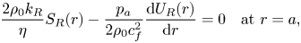 \begin{gather} \frac{2 \rho_0 k_{{R}}}{\eta} S_{{R}}(r) - \frac{p_{{a}}}{2 \rho_0 c_{{f}}^2} \frac{\mathrm{d} U_{{R}} (r)}{\mathrm{d} r} = 0 \quad \mathrm{at} \ r = a , \end{gather}
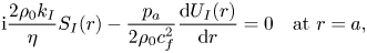 \begin{gather}\mathrm{i} \frac{2 \rho_0 k_{{I}}}{\eta} S_{{I}}(r) - \frac{p_{{a}}}{2 \rho_0 c_{{f}}^2} \frac{\mathrm{d} U_{{I}} (r)}{\mathrm{d} r} = 0 \quad \mathrm{at} \ r = a , \end{gather}
from the  $r$-component of the streaming velocity, and
 \begin{gather} \frac{\rho_0}{\eta} \frac{1}{r} S_{{R}}(r) + \frac{\rho_0}{\eta} \frac{\mathrm{d} S_{{R}}(r)}{\mathrm{d} r} - \frac{p_{{a}} k_{{R}}}{\rho_0 c_{{f}}^2} U_{{R}}(r) = 0 \quad \mathrm{at} \ r = a , \end{gather}
 \begin{gather}\mathrm{i} \frac{\rho_0}{\eta} \frac{1}{r} S_{{I}}(r) + \mathrm{i} \frac{\rho_0}{\eta} \frac{\mathrm{d} S_{{I}}(r)}{\mathrm{d} r} + \frac{p_{{a}} k_{{I}}}{\rho_0 c_{{f}}^2} U_{{I}}(r) = 0 \quad \mathrm{at} \ r = a , \end{gather}
from the  $z$-component.
Since (4.26) and (4.27) contain a factor of  $J_1 ( \xi _i r )$ that evaluates to zero for every $\xi _i$ at $r=a$, $S_{{R}}(r)$ and $S_{{I}}(r)$ are also zero at $r=a$ by definition. The constants $C_2$ and $C_4$ then follow trivially from their definitions (4.25) and (4.29), respectively:
 \begin{gather} C_2 = 0 , \end{gather}
 \begin{gather}C_4 = 0 . \end{gather}
From (4.49) and (4.51), we obtain
 \begin{equation} C_5 = \frac{\rm \pi}{2} \int_0^a x M_{{R}} (x) Y_0 ( - 2 \mathrm{i} k_{{R}} x) \, \mathrm{d}x + \frac{\rm \pi}{2} \frac{Y_1 ( - 2 \mathrm{i} k_{{R}} a)}{J_1 ( 2 \mathrm{i} k_{{R}} a)} \int_0^a x M_{{R}} (x) J_0 ( 2 \mathrm{i} k_{{R}} x) \, \mathrm{d}x, \end{equation}
 \begin{equation}C_7 = \frac{\rm \pi}{2} \int_0^a x M_{{I}} (x) Y_0 ( 2 k_{{I}} x) \, \mathrm{d}x - \frac{\rm \pi}{2} \frac{Y_1 ( 2 k_{{I}} a)}{J_1 ( 2 k_{{I}} a)} \int_0^a x M_{{I}} (x) J_0 ( 2 k_{{I}} x) \, \mathrm{d}x . \end{equation}
Exploiting, again, that  $S_{{R}}(r)$ and $S_{{I}}(r)$ are zero at $r=a$, together with boundary conditions (4.50) and (4.51), yields the last two constants in the following form:
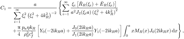 \begin{align} C_1 &= \frac{a}{\displaystyle\sum_{i=1}^{\infty} \xi_i^2 \left( \xi_i^2 + 4 k_{{R}}^2 \right)^{-2} } \left\{ \sum_{i=1}^{\infty} \frac{\xi_i \left[ \bar{R}_{{R}}(\xi_i) + \bar{E}_{{R}}(\xi_i) \right]}{a^2 J_2 (\xi_i a) \left( \xi_i^2 + 4 k_{{R}}^2 \right)^{2}} \right.\nonumber\\[-0.3pc] &\quad \left.+ \frac{\rm \pi}{4} \frac{p_{{a}} \eta k_{{R}}}{\rho_0^2 c_{{f}}^2} \left[ Y_0 (- 2 \mathrm{i} k_{{R}} a) + \frac{J_0 (2 \mathrm{i} k_{{R}} a)}{J_1 (2 \mathrm{i} k_{{R}} a)} Y_1 (- 2 \mathrm{i} k_{{R}} a) \right] \int_0^a x M_{{R}} (x) J_0 (2 \mathrm{i} k_{{R}} x) \, \mathrm{d}x \right\},\\[-1.7pc]\nonumber\end{align}
 \begin{align}C_3 &= \frac{a}{\displaystyle\sum_{i=1}^{\infty} \xi_i^2 \left( \xi_i^2 - 4 k_{{I}}^2 \right)^{-2} } \left\{ \sum_{i=1}^{\infty} \frac{\xi_i \left[ \bar{R}_{{I}}(\xi_i) + \bar{E}_{{I}}(\xi_i) \right]}{a^2 J_2 (\xi_i a) \left( \xi_i^2 - 4 k_{{I}}^2 \right)^{2}} \right.\nonumber\\[-0.3pc] &\quad \left. + \mathrm{i} \frac{\rm \pi}{4} \frac{p_{{a}} \eta k_{{I}}}{\rho_0^2 c_{{f}}^2} \left[ Y_0 ( 2 k_{{I}} a) - \frac{J_0 (2 k_{{I}} a)}{J_1 (2 k_{{I}} a)} Y_1 (2 k_{{I}} a) \right] \int_0^a x M_{{I}} (x) J_0 (2 k_{{I}} x) \, \mathrm{d}x \right\} . \end{align}
5. Streaming analysis
Here, we analyse the acoustic streaming for multiple combinations of material, geometrical and wave properties in a tube excited with two opposing decaying travelling waves that form a pseudo-standing wave. The analysis is performed in Mathematica 12.0 (Wolfram Research, Inc., 2019). The expressions (4.43), (4.44) and (4.47) for the velocity fields are used together with (4.26), (4.27), (4.41), (4.42), (F1), and the constants (4.52), (4.53), (4.54), (4.55), (4.56), (4.57). The integrals appearing in the transformed source terms  $\bar {R}_{{R}}(\xi _i)$, $\bar {R}_{{I}}(\xi _i)$, $\bar {E}_{{R}}(\xi _i)$, $\bar {E}_{{I}}(\xi _i)$, and in the expressions $U_{{R}} (r)$, $U_{{I}} (r)$, are evaluated numerically. The Mathematica Notebook file with the implementations of all necessary expressions for evaluation of arbitrary streaming fields is available as supplementary material at https://doi.org/10.1017/jfm.2020.1046. The infinite sums associated with the solution are truncated at $i_{{max}}$ (usually at $200$), at which the streaming velocity field is sufficiently converged. The limit is determined through convergence studies, information on which is given in appendix B.
In our analysis, we use water, oil, glycerol and air. The material properties of all four fluids are given in table 1.
Table 1. Material properties of the fluids used in the numerical analysis (Miner & Dalton Reference Miner and Dalton1953; Hirai & Eyring Reference Hirai and Eyring1958; Karlsen & Bruus Reference Karlsen and Bruus2015).
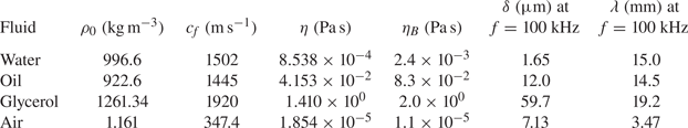
5.1. Definitions
To improve understanding of the fluid behaviour at the first order, we show, in figure 2, the real and the imaginary part of the wavenumber. In addition, the first-order pressure profile is given in figure 3, which indicates the symmetry of the pseudo-standing pressure wave with respect to the  $z=0$ plane. The amplitude decay relates to the imaginary part ( $k_{{I}}$) of the wavenumber, while the change of the wavelength with tube radius relates to the real part ( $k_{{R}}$) of the wavenumber. For the liquids, we will use a pressure amplitude of $100\ \textrm {kPa}$, which corresponds to the usual pressure amplitudes in acoustofluidic systems (Barnkob et al. Reference Barnkob, Augustsson, Laurell and Bruus2010). In the case of air, the usual pressure amplitude is much lower, up to $1\ \textrm {kPa}$ (Schuster & Matz Reference Schuster and Matz1940; Imani & Robert Reference Imani and Robert2015), which is the value that will be used for the results presented in appendix A.
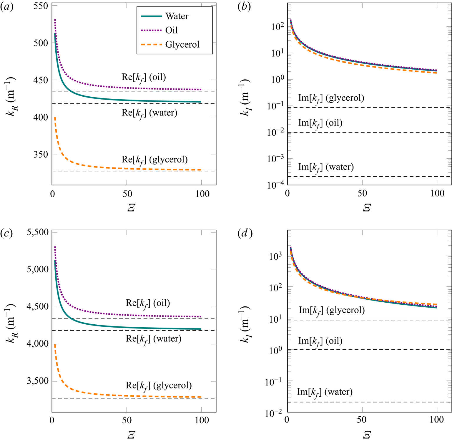
Figure 2. The real and imaginary parts of the wavenumber according to (3.31) and (3.32), respectively, for water, oil and glycerol: (a)  $k_R$ at $f = 100\ \textrm {kHz}$; (b) $k_I$ at $f = 100\ \textrm {kHz}$; (c) $k_R$ at $f = 1\ \textrm {MHz}$; (d) $k_I$ at $f = 1\ \textrm {MHz}$. The dimensionless ratio $\varXi = a / \delta$ represents the varying tube radius relative to the viscous boundary layer thickness. The real and imaginary parts of the wavenumber in an unbounded fluid domain $k_{{f}}$ are plotted for reference.
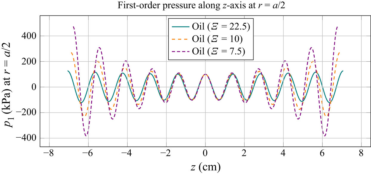
Figure 3. The first-order pressure in oil along the  $z$-axis, at $r=a/2$, for $f =100\ \textrm {kHz}$ and $p_{{a}} = 100\ \textrm {kPa}$. The dimensionless ratio $\varXi = a / \delta$ represents the varying tube radius relative to the viscous boundary layer thickness of $\delta = 12\ {\mathrm {\mu }}\textrm {m}$. For each radius of the tube, we plot the pressure in the range of $- 5 \lambda _{{R}} < z < 5 \lambda _{{R}}$, with $\lambda _{{R}} = 2 {\rm \pi}/ k_{{R}}$.
The first velocity node is positioned at  $z=0$, which is also a plane of symmetry of our pseudo-standing pressure wave (as indicated in figure 3). Since the fluid is viscous and bounded, the actual wavelength is defined as $\lambda _{{R}} = 2 {\rm \pi}/k_{{R}}$. The velocity node therefore repeats with a period of $\lambda _{{R}}/2$. The velocity antinode is in this case positioned at $z=\lambda _{{R}}/4$, and repeats with the same period as the node. Even though the fluids in our analysis are viscous (i.e. the imaginary part of the wavenumber $k$ is nonzero), we will use the acoustic wavelength of an unbounded ideal fluid $\lambda$, defined as $\lambda = c_{{f}}/f$, for a more generalized analysis.
The second-order solution is also symmetric about the  $z=0$ plane, which follows from the analysis of the $z$-dependency of the streaming velocity fields (4.43) and (4.47). The streaming patterns will therefore be analysed on the interval $0 \leq z \leq \lambda$. When a large-scale behaviour is analysed, the interval of analysis will be increased to $0 \leq z \leq 4 \lambda$.
In continuation, we will distinguish between two types of streaming vortices, namely Rayleigh streaming and Schlichting streaming. The Rayleigh streaming vortex denotes the flow from the velocity node towards the antinode near the axis of the tube, and the oppositely directed flow near the wall. The Schlichting streaming vortex represents the flow in the direction opposite to that of the Rayleigh streaming, and appears between the Rayleigh streaming and the wall. The two types of streaming are also shown in figure 4. The streaming vortices are analysed on a single  $rz$-plane, as the problem is axisymmetric. However, when three-dimensional geometry is considered these vortices extend through the whole range of $\theta$, namely $0 \leqslant \theta < 2 {\rm \pi}$, and are of toroidal shape. The two types of streaming vortices are boundary-driven, and are normally confined between a velocity nodal plane and antinodal plane of an acoustic field. However, we will also encounter streaming driven by the decaying travelling wave grazing the wall (Nyborg Reference Nyborg1965, p. 274). This type of large-scale (with respect to $\lambda$) streaming will be called Eckart-like streaming, after Eckart (Reference Eckart1948), who theoretically investigated the streaming driven by the attenuation of a travelling wave in the bulk of a fluid, extending over several acoustic wavelengths in the direction of the wave propagation. This happens, for example, when the waveguide of an acoustic beam is wider than the acoustic wavelength (Boluriaan & Morris Reference Boluriaan and Morris2003).
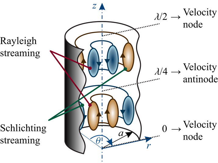
Figure 4. The terminology used for different types of streaming vortices. Rayleigh streaming denotes the fluid flow from the velocity node to the antinode near the axis of the tube, and the flow in the opposite direction near the wall. Schlichting streaming denotes the flow in the direction opposite to that of the Rayleigh streaming.
We will often refer to the ratio of a tube radius to the thickness of the viscous boundary layer, i.e. the quantity
 \begin{equation} \varXi = \frac{a}{\delta} . \end{equation}
The critical ratio  $\varXi _{{S}}$, as indicated in figure 5, denotes the transition between the Rayleigh-plus-Schlichting streaming regime to the Schlichting-only streaming regime. It is defined as the value of $\varXi$ at which the axial component of the streaming velocity changes direction, at $z=\lambda _{{R}}/8$. We will also use another dimensionless parameter, the ratio of the acoustic wavelength to the tube radius, i.e. the quantity
 \begin{equation} \varLambda = \frac{\lambda}{a} . \end{equation}
The critical ratio  $\varLambda _{{E}}$ signifies the transition between the Rayleigh-plus-Schlichting streaming regime to the Eckart-plus-Schlichting regime, and is defined as the value of $\varLambda$ at which the axial component of the streaming velocity changes direction, at $z=3 \lambda _{{R}}/8$, while $\varXi$ is sufficiently above $\varXi _{{S}}$ so that the transition associated with $\varXi _{{S}}$ does not interfere. The specified critical values of $\varXi$ and $\varLambda$, depicted in figure 5, are problem-specific parameters, and their dependency on the material properties and on the excitation frequency will be investigated in the following sections. The superscript $\square ^{{M}}$ indicates that the ratio is determined via the average mass transport velocity (4.47), while critical ratios without the superscript are determined via the Eulerian streaming velocity (4.43).

Figure 5. Visual explanation of the critical values of  $\varXi = a/\delta$ and $\varLambda =\lambda /a$ used in the analysis. In the case of $\varXi < \varXi _{{S}}$ the Rayleigh streaming disappears completely, and only the Schlichting streaming remains. This happens when the axial component of the streaming at the axis, at $z=\lambda _{{R}}/8$, changes direction. When $\varLambda < \varLambda _{{E}}$, large-scale Eckart-like streaming begins to develop near the axis of the tube. The ratio $\varLambda _{{E}}$ is defined as the value of $\varLambda$ at which the axial streaming velocity at the axis, evaluated at $z=3 \lambda _{{R}}/8$, changes direction, while $\varXi > \varXi _{{S}}$.
5.2. The evolution of streaming patterns
Figure 6 shows the evolution of the average mass transport velocity patterns inside an oil-filled tube with respect to the decreasing tube radius at a constant frequency of  $f=100\ \textrm {kHz}$, which corresponds to a viscous boundary layer thickness of $\delta = 12\ {\mathrm {\mu }}\textrm {m}$ and an acoustic wavelength of $\lambda = 14.45\ \textrm {mm}$. We observe a qualitative change in the behaviour. First, at $a=270\ {\mathrm {\mu }}\textrm {m}$ ( $\varXi = 22.5$), in figure 6(a), we see a combination of smaller Schlichting vortices at the wall and dominant Rayleigh streaming vortices that agree with well-known experiments (see Andrade Reference Andrade1931); i.e. the fluid flows from the velocity node towards the antinode near the axis of the tube and in the opposite direction near the wall. When the radius is decreased to $a=120\ {\mathrm {\mu }}\textrm {m}$ ( $\varXi = 10$) and $a=90\ {\mathrm {\mu }}\textrm {m}$ ( $\varXi = 7.5$), we observe the expansion of the Schlichting vortices near the wall, in addition to the shrinking of the Rayleigh vortices (figure 6b,c). Further decreasing the radius to $a=70\ {\mathrm {\mu }}\textrm {m}$ ( $\varXi = 5.83$), $a=50\ {\mathrm {\mu }}\textrm {m}$ ( $\varXi = 4.17$) and $a=40\ {\mathrm {\mu }}\textrm {m}$ ( $\varXi = 3.33$) reveals the disappearance of the Rayleigh streaming, while the Schlichting streaming spreads throughout the whole radius of the tube (figure 6d–f). Figure 7 gives the Eulerian streaming velocity patterns corresponding to the same cases as presented in figure 6.
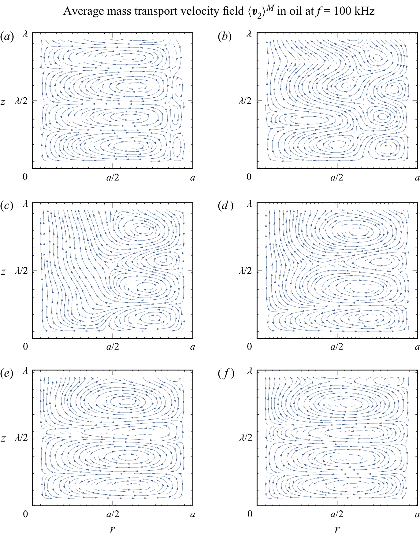
Figure 6. The average mass transport velocity patterns in oil, for a tube radius of (a)  $a=270\ {\mathrm {\mu }}\textrm {m}$ $(\varXi = 22.5)$, (b) $a=120\ {\mathrm {\mu }}\textrm {m}$ $(\varXi = 10)$, (c) $a=90\ {\mathrm {\mu }}\textrm {m}$ $(\varXi = 7.5)$, (d) $a=70\ {\mathrm {\mu }}\textrm {m}$ $(\varXi = 5.83)$, (e) $a=50\ {\mathrm {\mu }}\textrm {m}$ $(\varXi = 4.17)$ and (f) $a=40\ {\mathrm {\mu }}\textrm {m}$ $(\varXi = 3.33)$, for $f = 100\ \textrm {kHz}$. The corresponding acoustic wavelength is $\lambda = 14.45\ \textrm {mm}$, while the actual wavelength is $14.14\ \textrm {mm} \geqslant \lambda _{{R}} \geqslant 12.67\ \textrm {mm}$. The viscous boundary layer has a thickness of $\delta = 12\ {\mathrm {\mu }}\textrm {m}$. The first velocity node is at $z=0$, while the first velocity antinode appears at $z = \lambda _{{R}} / 4$. Arrows indicate the direction of the flow.
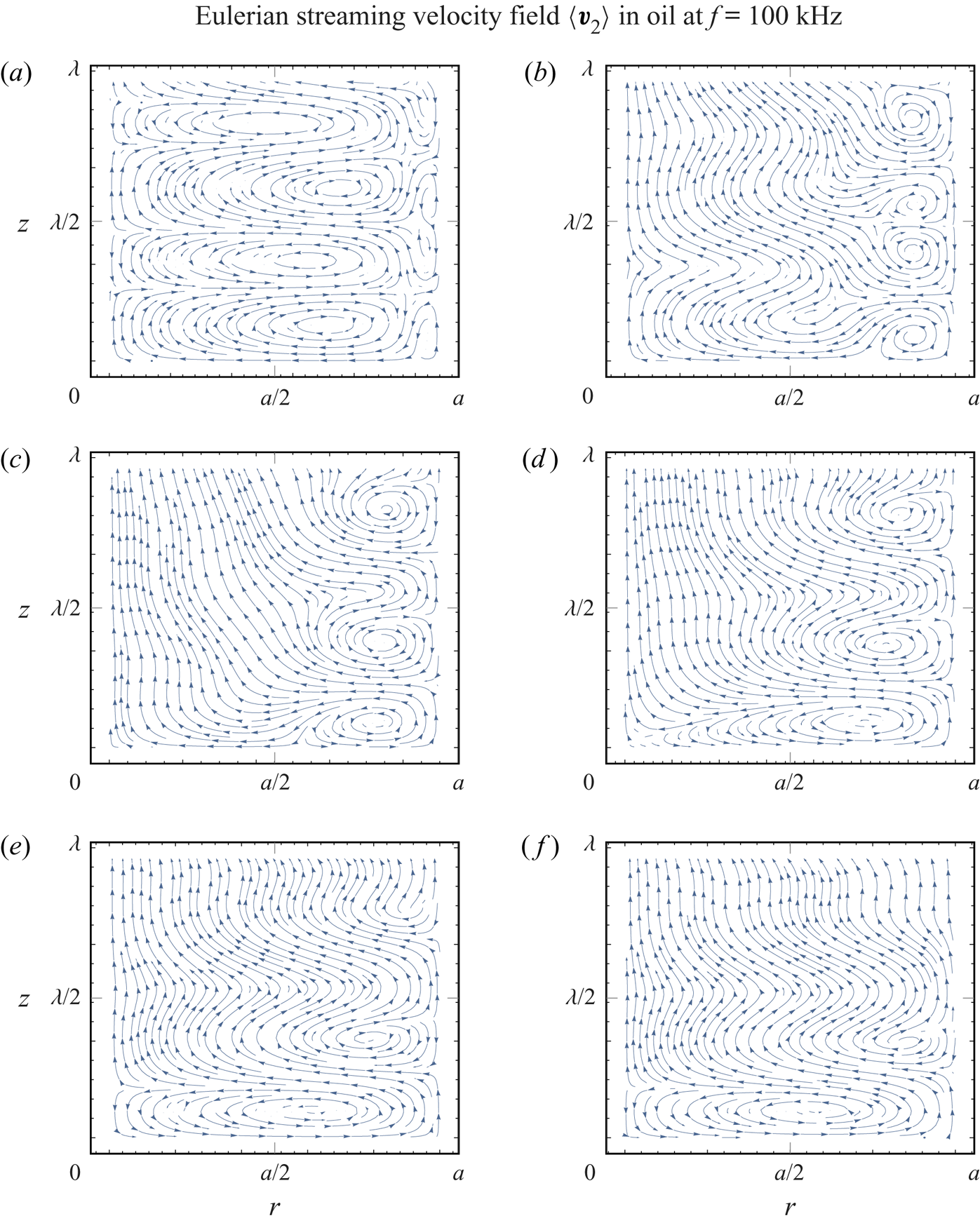
Figure 7. The Eulerian streaming velocity patterns in oil, for a tube radius of (a)  $a=270\ {\mathrm {\mu }}\textrm {m}$ $(\varXi = 22.5)$, (b) $a=120\ {\mathrm {\mu }}\textrm {m}$ $(\varXi = 10)$, (c) $a=90\ {\mathrm {\mu }}\textrm {m}$ $(\varXi = 7.5)$, (d) $a=70\ {\mathrm {\mu }}\textrm {m}$ $(\varXi = 5.83)$, (e) $a=50\ {\mathrm {\mu }}\textrm {m}$ $(\varXi = 4.17)$ and (f) $a=40\ {\mathrm {\mu }}\textrm {m}$ $(\varXi = 3.33)$, for $f = 100\ \textrm {kHz}$. The corresponding acoustic wavelength is $\lambda = 14.45\ \textrm {mm}$, while the actual wavelength is $14.14\ \textrm {mm} \geqslant \lambda _{{R}} \geqslant 12.67\ \textrm {mm}$. The viscous boundary layer has a thickness of $\delta = 12\ {\mathrm {\mu }}\textrm {m}$. The first velocity node is at $z=0$, while the first velocity antinode appears at $z = \lambda _{{R}} / 4$. Arrows indicate the direction of the flow.
We observe that the periodicity of the streaming pattern with respect to the  $z$-axis, and within the first few vortices, is very distinct when only a single type of streaming is present (e.g. in figure 6a,e,f), compared to the situations where Rayleigh and Schlichting streaming vortices coexist (e.g. in figure 6b–d). The first-order acoustic fields are periodic in $z$, but their amplitudes are exponential functions of $z$. Then, at the second order, the time-averaging of the products of first-order fields leads to the decoupling of the sinusoidal and exponential $z$-dependencies from products into sums. This results in the observed non-periodic behaviour along the $z$-axis at the second order.
The streaming patterns in figure 6 are plotted for one ideal wavelength ( $\lambda$) along the $z$-axis. However, we can observe that the streaming patterns and the actual wavelength ( $\lambda _{{R}}$) shrink along the $z$-axis with the decrease of $\varXi$. This follows from the increase of $k_{{R}}$ with the decrease of $\varXi$, which is shown in figure 2.
In figures 8 and 9, we look at the axial and radial velocity profiles, respectively, corresponding to the cases analysed in figures 6 and 7. The superscripts  $\square ^z$ and $\square ^r$ denote the $z$- and $r$-components of the velocity, respectively (e.g. $v_2^z = \left \langle \boldsymbol {v}_2 \right \rangle \boldsymbol {\cdot } \boldsymbol {e}_z$). We analyse profiles of four different velocities: $v_2^z$ and $v_2^r$ relate to the Eulerian streaming velocity $\left \langle \boldsymbol {v}_2 \right \rangle$; $v_2^{{L} z}$ and $v_2^{{L} r}$ relate to the Lagrangian streaming velocity $\left \langle \boldsymbol {v}_2 \right \rangle ^{{L}}$; $v_2^{{M} z}$ and $v_2^{{M} r}$ relate to the average mass transport velocity $\left \langle \boldsymbol {v}_2 \right \rangle ^{{M}}$; and we also plot $v_2^{{S} z}$ and $v_2^{{S} r}$, which correspond to the model by Schuster & Matz (Reference Schuster and Matz1940), given as (G1) in appendix G. The axial velocity profiles, in figure 8, are plotted through the radius of the tube, at $z=\lambda _{{R}}/8$, i.e. at the middle of the first streaming vortex along the $z$-axis, starting from $z=0$. We observe that the magnitudes of $v_2^z$, $v_2^{{L} z}$ and $v_2^{{M} z}$ are largest when one type of streaming vortex is dominant, i.e. at $\varXi =22.5$ ( $a=270\ {\mathrm {\mu }}\textrm {m}$) and at $\varXi =3.33$ ( $a=40\ {\mathrm {\mu }}\textrm {m}$). The profiles are, outside the viscous boundary layer, well aligned with $v_2^{{S} z}$ at $\varXi =22.5$, but the difference becomes more and more significant as the ratio $\varXi$ decreases, which is reasonable since Schuster & Matz (Reference Schuster and Matz1940) assumed $\varXi \gg 1$. After reaching a certain critical ratio $\varXi$ (referred to later as $\varXi _{{S}}$), the change of the direction of the $z$-component of the streaming velocity at $r=0$ indicates the qualitative change in the behaviour which is not captured by the model of Schuster & Matz (Reference Schuster and Matz1940). Namely, the Schlichting streaming vortex spreads throughout the whole radius of the tube, as seen in figure 8(e,f).
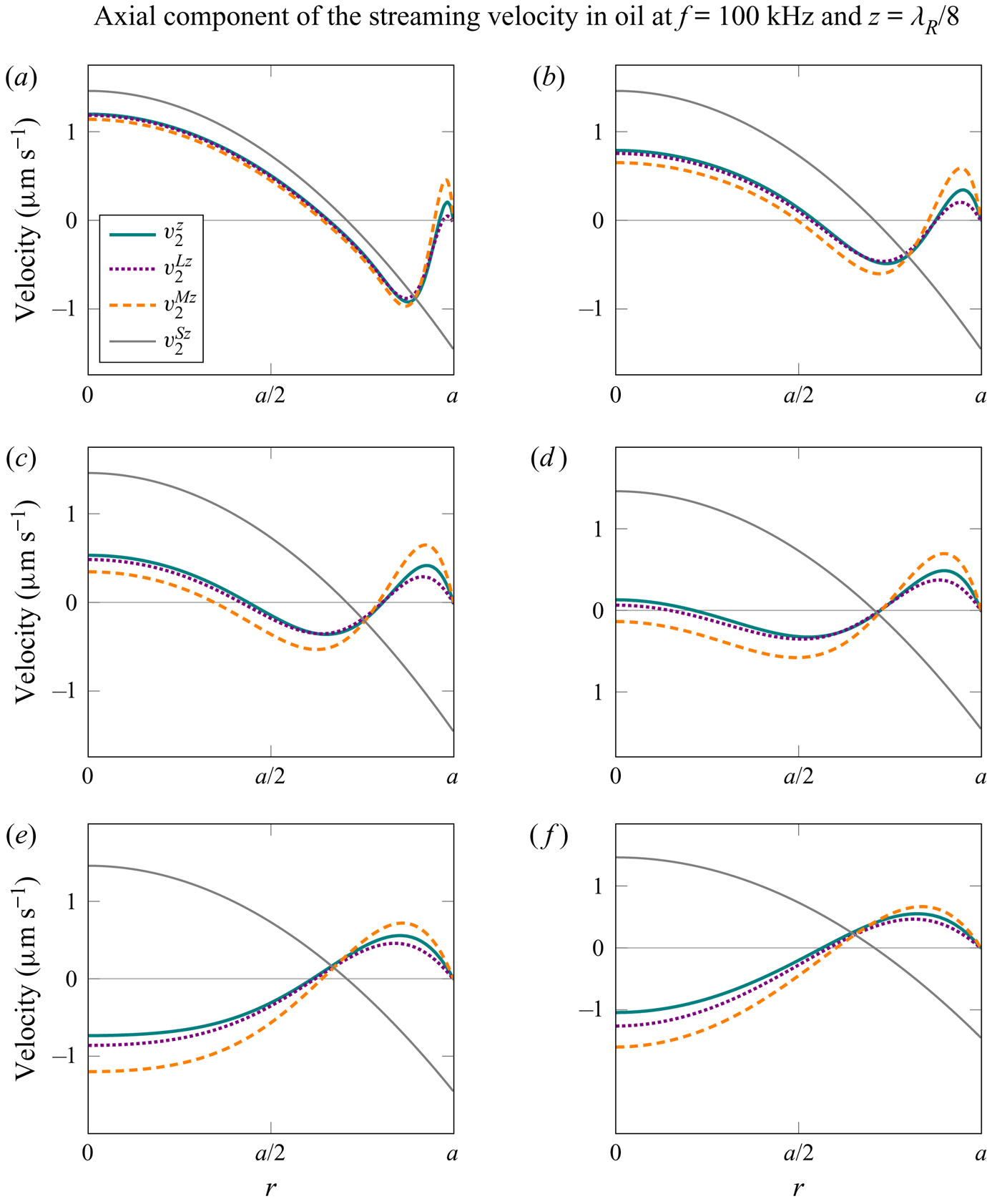
Figure 8. The analysis of the axial velocity profiles in oil, at  $z=\lambda _{{R}}/8$, for a tube radius of (a) $a=270\ {\mathrm {\mu }}\textrm {m}$ $(\varXi = 22.5)$, (b) $a=120\ {\mathrm {\mu }}\textrm {m}$ $(\varXi = 10)$, (c) $a=90\ {\mathrm {\mu }}\textrm {m}$ $(\varXi = 7.5)$, (d) $a=70\ {\mathrm {\mu }}\textrm {m}$ $(\varXi = 5.83)$, (e) $a=50\ {\mathrm {\mu }}\textrm {m}$ $(\varXi = 4.17)$ and (f) $a=40\ {\mathrm {\mu }}\textrm {m}$ $(\varXi = 3.33)$, for $f = 100\ \textrm {kHz}$ and $p_{{a}} = 100\ \textrm {kPa}$. Also shown for comparison are the $z$-components of the Eulerian streaming velocity, $v_2^z$, the Lagrangian streaming velocity, $v_2^{{L} z}$, the average mass transport velocity, $v_2^{{M} z}$, and a reference velocity (evaluated at $z=\lambda /8$) from Schuster & Matz (Reference Schuster and Matz1940), $v_2^{{S} z}$, given as (G1) in appendix G.

Figure 9. Analysis of the radial velocity profiles in oil, at  $r=a/2$, for a tube radius of (a) $a=270\ {\mathrm {\mu }}\textrm {m}$ $(\varXi = 22.5)$, (b) $a=120\ {\mathrm {\mu }}\textrm {m}$ $(\varXi = 10)$, (c) $a=90\ {\mathrm {\mu }}\textrm {m}$ $(\varXi = 7.5)$, (d) $a=70\ {\mathrm {\mu }}\textrm {m}$ $(\varXi = 5.83)$, (e) $a=50\ {\mathrm {\mu }}\textrm {m}$ $(\varXi = 4.17)$ and (f) $a=40\ {\mathrm {\mu }}\textrm {m}$ $(\varXi = 3.33)$, for $f = 100\ \textrm {kHz}$ and $p_{{a}} = 100\ \textrm {kPa}$. Also shown for comparison are the $r$-components of the Eulerian streaming velocity, $v_2^r$, the Lagrangian streaming velocity, $v_2^{{L} r}$, the average mass transport velocity, $v_2^{{M} r}$, and a reference velocity from Schuster & Matz (Reference Schuster and Matz1940), $v_2^{{S} r}$, given as (G1) in appendix G.
The analysis of the critical ratios  $\varXi _{{S}}^{{M}}$ and $\varXi _{{S}}$ at $f=100\ \textrm {kHz}$, in figures 10 and 11, shows that the ratios are invariant with respect to the fluid properties, as they are the same for water, oil and glycerol. Figures 10 and 11 show the evolution of the $z$-components of the Eulerian streaming velocity and average mass transport velocity, respectively, at $r = 0$. Both evaluations are done at $z = \lambda _{{R}}/8$, (i.e. the middle of the first streaming vortex along the $z$-axis). The ratios $\varXi _{{S}}^{{M}}$ and $\varXi _{{S}}$ are defined as the values of $\varXi$ at which the Eulerian streaming velocity and the average mass transport velocity, respectively, in the centre of the tube change sign, as this indicates the disappearance of the Rayleigh streaming. The critical ratios resulting from the discussed analysis are $\varXi _{{S}}^{{M}}=6.2$ and $\varXi _{{S}}=5.6$.

Figure 10. The  $z$-component of the average mass transport velocity, $v_2^{{M} z}$, at $r = 0$ and $z = \lambda _{{R}} / 8$, depending on the normalized tube radius $\varXi = a / \delta$, for $f = 100\ \textrm {kHz}$ and $p_{{a}} = 100\ \textrm {kPa}$. The critical ratio $\varXi _{{S}}^{{M}}$ is defined as the value of $\varXi$ at which $v_2^{{M} z}$ changes direction. The velocity magnitudes (S. & M.) calculated with the model of Schuster & Matz (Reference Schuster and Matz1940) are given for reference (see (G2) in appendix G).
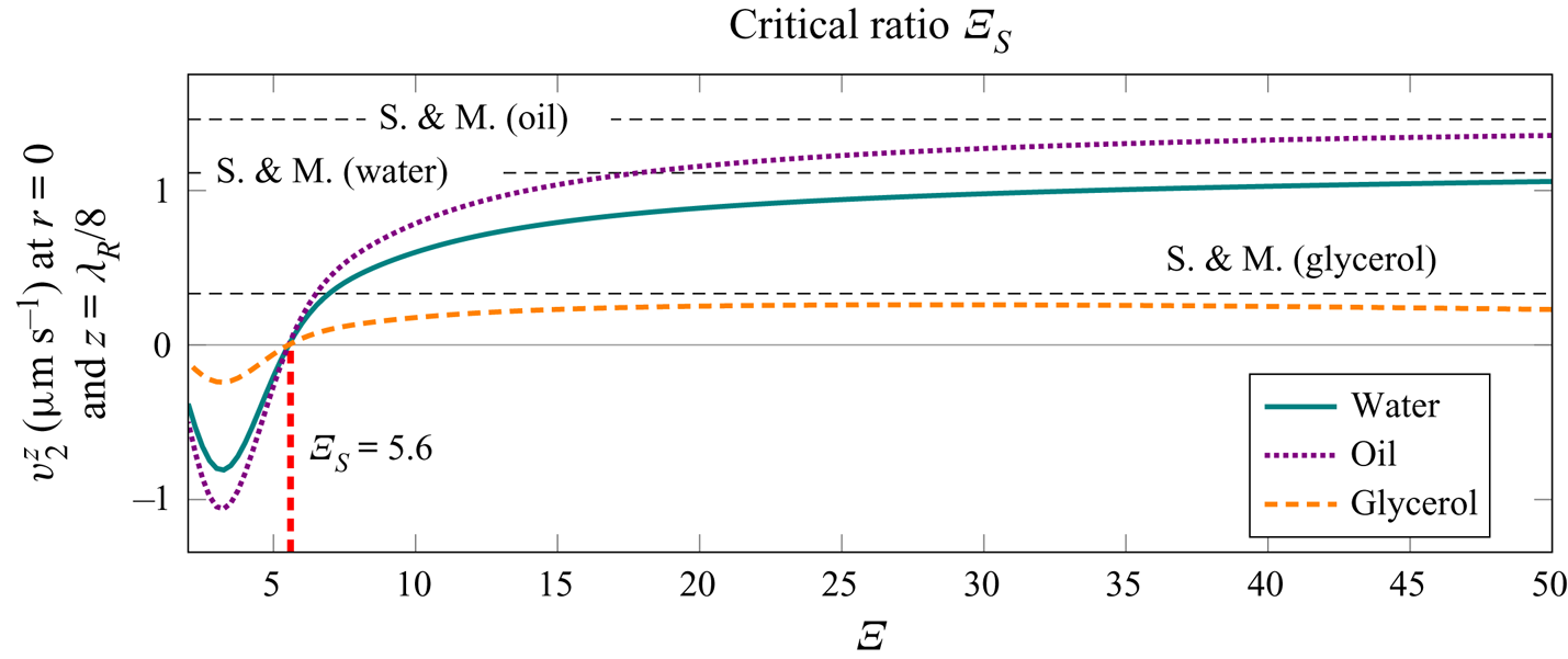
Figure 11. The  $z$-component of the Eulerian streaming velocity, $v_2^z$, at $r = 0$ and $z = \lambda _{{R}} / 8$, depending on the normalized tube radius $\varXi = a / \delta$, for $f = 100\ \textrm {kHz}$ and $p_{{a}} = 100\ \textrm {kPa}$. The critical ratio $\varXi _{{S}}$ is defined as the value of $\varXi$ at which $v_2^z$ changes direction. The velocity magnitudes (S. & M.) calculated with the model of Schuster & Matz (Reference Schuster and Matz1940) are given for reference (see (G2) in appendix G).
In addition, figure 11 shows the values for the streaming velocity magnitude using the model of Schuster & Matz (Reference Schuster and Matz1940). The equation for the velocity magnitude is given as (G2) in appendix G. We observe that the simplified model (Schuster & Matz Reference Schuster and Matz1940) matches well with our solution when the radius of the tube is large relative to the thickness of the viscous boundary layer, i.e. for  $\varXi \gg 1$. However, for $\varXi \lesssim 20$ the simplified model (Schuster & Matz Reference Schuster and Matz1940) is not valid anymore.
5.3. Effect of the acoustic wavelength on the streaming
The analysis of the streaming patterns at higher frequencies and for the same range of  $\varXi$ reveals no significant differences in the streaming patterns, assuming $\varLambda = \lambda / a \gg 1$ and consequently $\lambda / \delta \gg 1$. However, for glycerol, the tube radius corresponding to $\varXi = 22.5$ (the largest value of $\varXi$ analysed in figure 6) can approach the wavelength at frequencies that are attainable in microfluidic devices. Keeping $\varXi$ constant at $22.5$ and reducing $\varLambda$ through manipulation of the frequency and radius leads to the change of the $z$-component of the streaming velocity at $z=3 \lambda _{{R}} / 8$, as depicted in figure 12. This eventually leads to the change of the direction of the analysed velocity, which signals the appearance of large-scale Eckart-like streaming, at $\varLambda =\varLambda _{{E}}$. The critical ratios based on the average mass transport velocity and the Eulerian streaming velocity are $\varLambda _{{E}}^{{M}} = 3.1$ and $\varLambda _{{E}} = 3.5$, respectively. In addition, we observe that the streaming velocity is constant with respect to $\varLambda$, for $\varLambda \gtrsim 20$. Additional studies reveal that $\varLambda _{{E}}^{{M}}$ and $\varLambda _{{E}}$ are not invariant with respect to $\varXi$, and increase as $\varXi$ decreases.
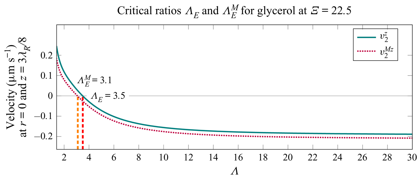
Figure 12. The  $z$-components of the average mass transport velocity and the Eulerian streaming velocity, $v_2^{{M} z}$ and $v_2^z$, respectively, in glycerol. The velocities depend on the normalized acoustic wavelength $\varLambda = \lambda / a$, which is varied by varying the frequency ( $10.441\ \textrm {MHz} \geq f \geq 22.738\ \textrm {kHz}$) and the radius of the tube ( $131.4\ \mathrm {\mu }\textrm {m} \leq a \leq 2814.6\ \mathrm {\mu }\textrm {m}$), keeping $\varXi$ constant at $22.5$. The velocities are evaluated at $r = 0$ and $z = 3 \lambda _{{R}} / 8$, for $p_{{a}} = 100\ \textrm {kPa}$. The critical ratios $\varLambda _{{E}}^{{M}}$ and $\varLambda _{{E}}$ are defined as the values of $\varLambda$ at which $v_2^{{M} z}$ and $v_2^z$, respectively, change direction.
The transition from the Rayleigh-plus-Schlichting streaming regime at  $\varLambda > \varLambda _{{E}}^{{M}}$ to the Eckart-plus-Schlichting regime at $\varLambda < \varLambda _{{E}}^{{M}}$ is also studied through the evolution of the average mass transport velocity patterns in figure 13. The ratio $\varXi$ is kept constant at $22.5$, while the ratio $\varLambda$ is varied through adjustment of the frequency and the radius of the tube. The resulting patterns are qualitatively different from the patterns in oil shown in figure 6. The difference is minute for the moderately small $\varLambda$ of $10$ in figure 13(a), and becomes very prominent as $\varLambda$ is decreased all the way to $\varLambda = 1$ in figure 13(f), where the Eckart-like streaming dominates near the axis, in addition to small Schlichting vortices near the wall. The large-scale nature of the Eckart-like streaming is further demonstrated in figure 14, where the interval of the analysis is increased from $0\leq z \leq \lambda$ to $0 \leq z \leq 4 \lambda$.
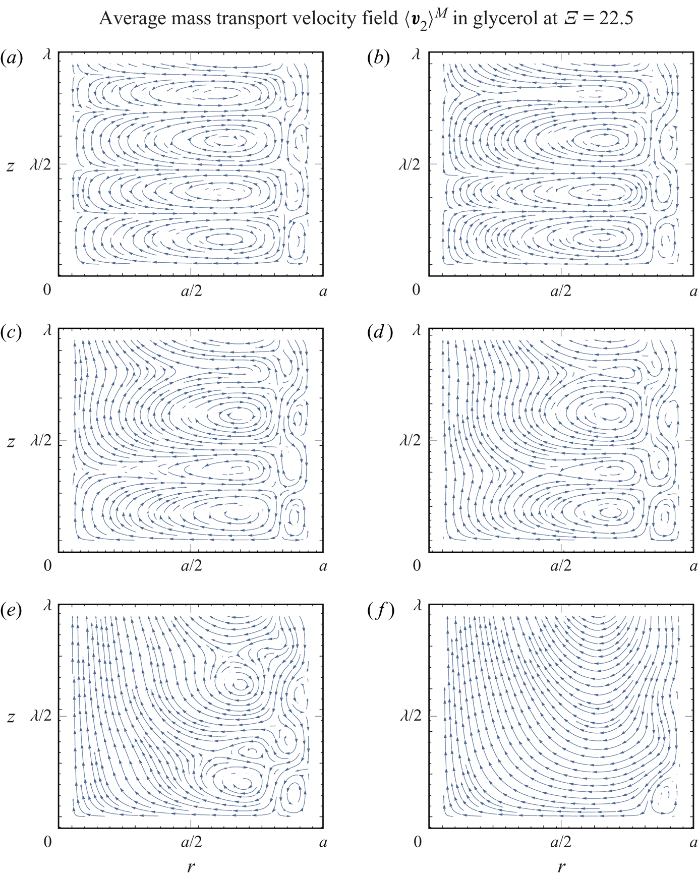
Figure 13. The average mass transport velocity patterns in glycerol, for (a)  $\varLambda =10$, (b) $\varLambda =4$, (c) $\varLambda =3$, (d) $\varLambda =2.5$, (e) $\varLambda =2$ and (f) $\varLambda =1$. The patterns depend on the normalized acoustic wavelength $\varLambda = \lambda / a$, which is varied by varying the frequency ( $204.644\ \textrm {kHz} \leq f \leq 20.464\ \textrm {MHz}$) and the radius of the tube ( $938.2\ \mathrm {\mu }\textrm {m} \geq a \geq 93.8\ \mathrm {\mu }\textrm {m}$), keeping $\varXi$ constant at $22.5$. The first velocity node is at $z=0$, while the first velocity antinode appears at $z = \lambda _{{R}} / 4$. Arrows indicate the direction of the flow.
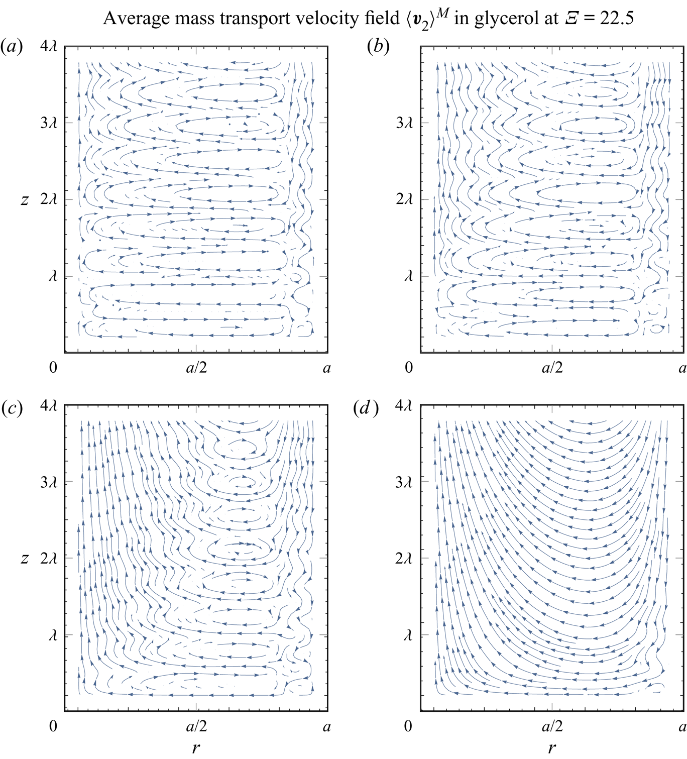
Figure 14. The average mass transport velocity patterns in glycerol, for (a)  $\varLambda =10$, (b) $\varLambda =4$, (c) $\varLambda =2.5$ and (d) $\varLambda =1$. The patterns depend on the normalized acoustic wavelength $\varLambda = \lambda / a$, which is varied by varying the frequency ( $204.644\ \textrm {kHz} \leq f \leq 20.464\ \textrm {MHz}$) and the radius of the tube ( $938.2\ \mathrm {\mu }\textrm {m} \geq a \geq 93.8\ \mathrm {\mu }\textrm {m}$), keeping $\varXi$ constant at $22.5$. The first velocity node is at $z=0$, while the first velocity antinode appears at $z = \lambda _{{R}} / 4$. The patterns are plotted on the interval $0 \leq z \leq 4 \lambda$ to reveal the large-scale nature of the streaming flow. Arrows indicate the direction of the flow.
The streaming patterns at  $\varLambda < \varLambda _{{E}}^{{M}}$, e.g. figure 13(f), reveal that the streaming flow at the axis of the tube is directed towards the incoming decaying travelling wave and in the opposite direction near the wall. This behaviour is in agreement with the flow in the case of a travelling wave which grazes the wall (Nyborg Reference Nyborg1965, p. 274). Since the acoustic wave propagates through the whole cross-section of the tube, the described behaviour differs from the regular Eckart streaming (Eckart Reference Eckart1948), where the acoustic source is smaller than the tube cross-section.
5.4. Contribution of the compressibility of the streaming flow
Streaming flow is sometimes assumed incompressible in similar situations (e.g. Schuster & Matz Reference Schuster and Matz1940; Doinikov et al. Reference Doinikov, Thibault and Marmottant2017), which means that the second-order continuity equation (4.1), namely  $\boldsymbol {\nabla } \boldsymbol {\cdot } \left \langle \boldsymbol {\boldsymbol {v}}_2 \right \rangle = -1/\rho _0 \boldsymbol {\nabla } \boldsymbol {\cdot } \left \langle \rho _1 \boldsymbol {v}_1 \right \rangle$, is simplified to $\boldsymbol {\nabla } \boldsymbol {\cdot } \left \langle \boldsymbol {\boldsymbol {v}}_2 \right \rangle = 0$. Nevertheless, the validity of this assumption is not clear, and the effect of compressibility at the second order, as remarked by Menguy & Gilbert (Reference Menguy and Gilbert2000), still poses one of the main unresolved issues in the field of acoustic streaming.
Here, we use the solution for  $\left \langle \boldsymbol {v}_2 \right \rangle$ that results if the aforementioned continuity equation (4.1) is replaced by $\boldsymbol {\nabla } \boldsymbol {\cdot } \left \langle \boldsymbol {\boldsymbol {v}}_2 \right \rangle = 0$ (this renders the irrotational part of the streaming velocity, namely $\boldsymbol {\nabla } \varphi _2$, zero, and changes the remaining constants $C_1$ and $C_3$).
Since the concept of the average mass transport velocity does not arise naturally in this case, i.e. it is not divergence-free by definition, we plot only the Eulerian streaming velocity patterns, in figure 15. Comparison with figures 6 and 7 shows that the incompressible Eulerian streaming velocity patterns in figure 15 better resemble the average mass transport velocity patterns from figure 6 than the corresponding Eulerian streaming velocity patterns from figure 7. Additionally, in the transition phase, when Rayleigh streaming is gradually disappearing (figure 15b–d), the incompressible patterns preserve the periodicity with respect to the  $z$-axis better than the patterns of the compressible solution.
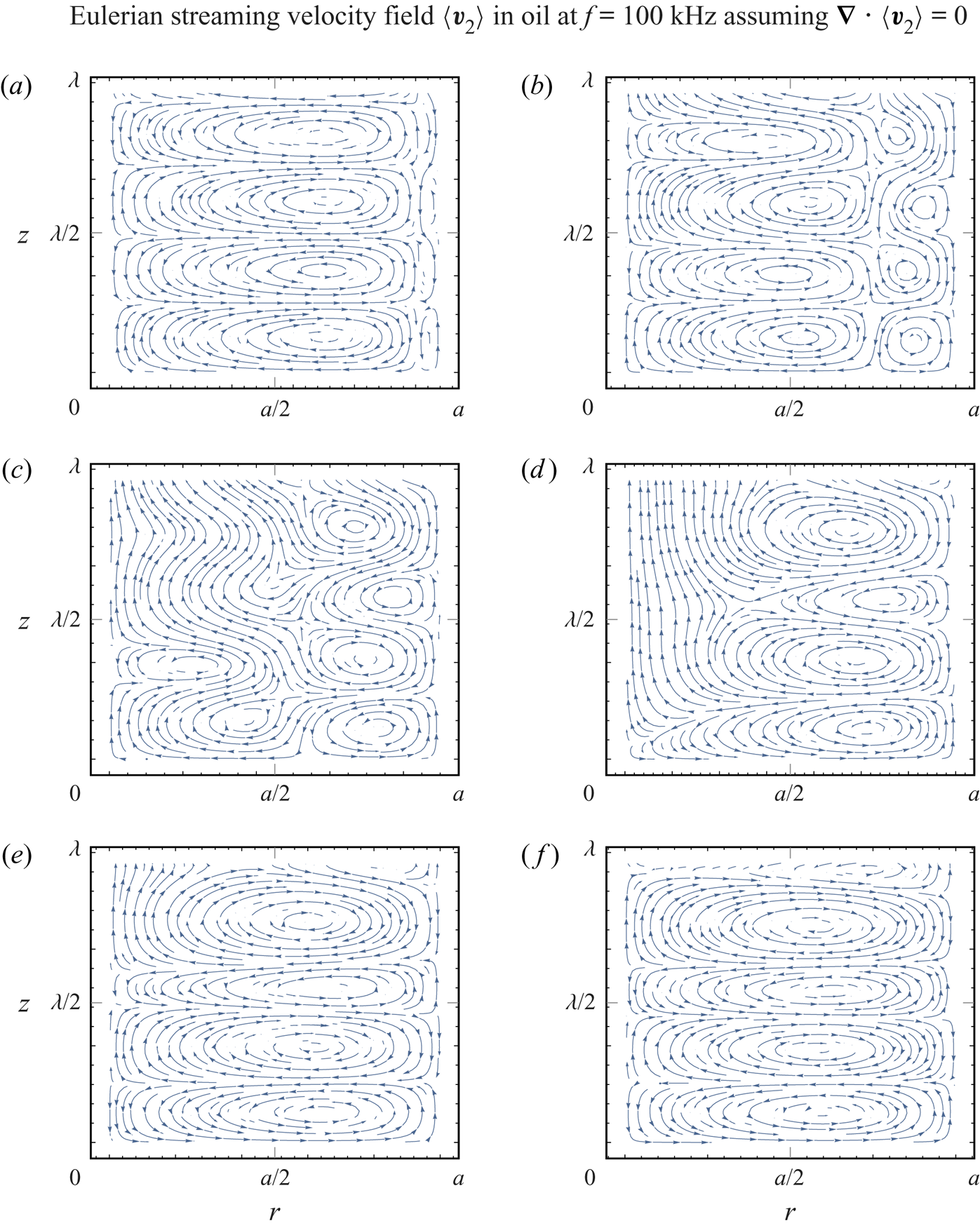
Figure 15. The Eulerian streaming velocity patterns in oil, using the Eulerian divergence-free formulation, i.e.  $\boldsymbol {\nabla } \boldsymbol {\cdot } \left \langle \boldsymbol {v}_2 \right \rangle = 0$, for a tube radius of (a) $a=270\ {\mathrm {\mu }}\textrm {m}$ $(\varXi = 22.5)$, (b) $a=120\ {\mathrm {\mu }}\textrm {m}$ $(\varXi = 10)$, (c) $a=90\ {\mathrm {\mu }}\textrm {m}$ $(\varXi = 7.5)$, (d) $a=70\ {\mathrm {\mu }}\textrm {m}$ $(\varXi = 5.83)$, (e) $a=50\ {\mathrm {\mu }}\textrm {m}$ $(\varXi = 4.17)$ and (f) $a=40\ {\mathrm {\mu }}\textrm {m}$ $(\varXi = 3.33)$, for $f = 100\ \textrm {kHz}$. The corresponding acoustic wavelength is $\lambda = 14.45\ \textrm {mm}$, while the actual wavelength is $14.14\ \textrm {mm} \geqslant \lambda _{{R}} \geqslant 12.67\ \textrm {mm}$. The viscous boundary layer has a thickness of $\delta = 12\ {\mathrm {\mu }}\textrm {m}$. The first velocity node is at $z=0$, while the first velocity antinode appears at $z = \lambda _{{R}} / 4$. Arrows indicate the direction of the flow.
With the modified solution for the incompressible streaming flow, we analyse the critical ratio  $\varXi _{{S}}$. The results, in figure 16, indicate that the compressibility slightly decreases $\varXi _{{S}}$, as the incompressible solution yields $\varXi _{{S}} = 5.8$, compared to the value $\varXi _{{S}} = 5.6$ of the compressible solution (figure 11).
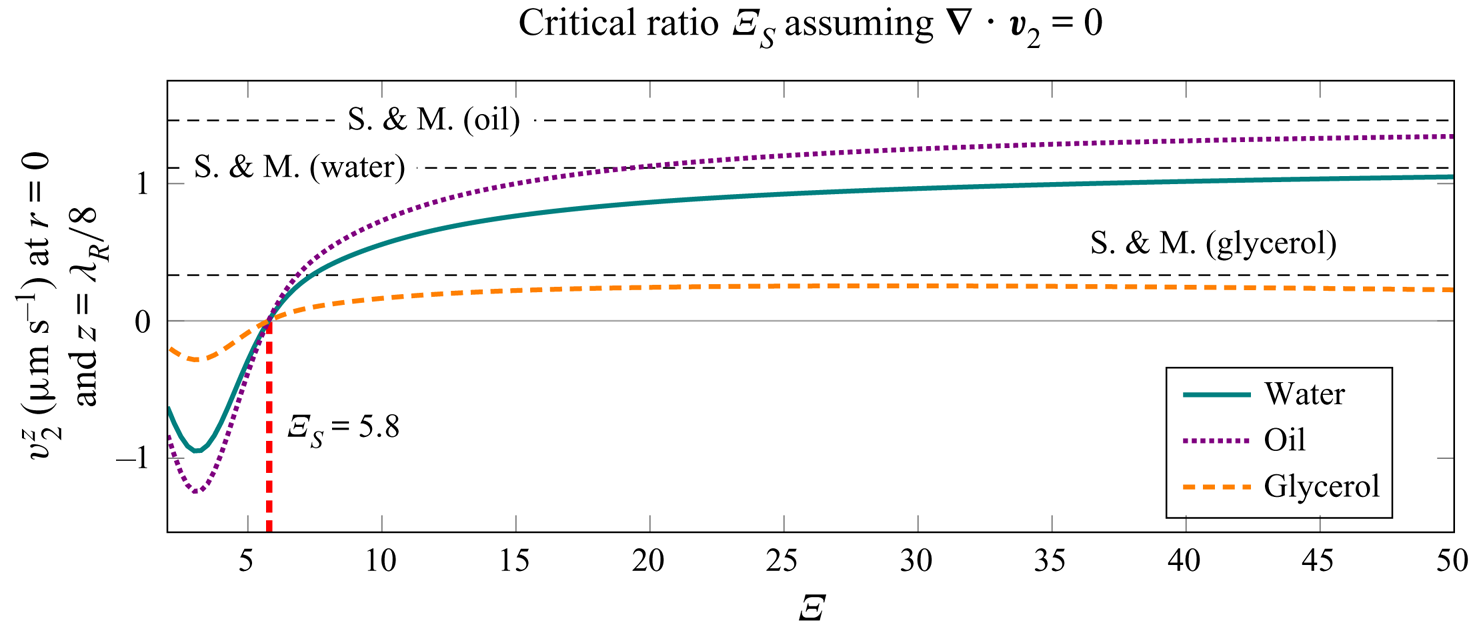
Figure 16. The  $z$-component of the Eulerian streaming velocity, $v_2^z$, using the divergence-free formulation, i.e. $\boldsymbol {\nabla } \boldsymbol {\cdot } \left \langle \boldsymbol {v}_2 \right \rangle = 0$, at $r = 0$ and $z = \lambda _{{R}} / 8$, depending on the normalized tube radius $\varXi = a / \delta$, for $f = 100\ \textrm {kHz}$ and $p_{{a}} = 100\ \textrm {kPa}$. The critical ratio $\varXi _{{S}}$ is defined as the value of $\varXi$ at which $v_2^z$ changes direction. The velocity magnitudes (S. & M.) calculated with the model of Schuster & Matz (Reference Schuster and Matz1940) are given for reference (see (G2) in appendix G).
5.5. Contribution of individual streaming source terms
We repeat the average mass transport velocity pattern analysis from figure 6, but this time we set  $E_{{R}}(r) = E_{{I}}(r) = 0$, i.e. we omit the usually neglected source term in the streaming equations (4.2) (see e.g. Rayleigh Reference Rayleigh1884; Schlichting Reference Schlichting1932; Lighthill Reference Lighthill1978; Doinikov et al. Reference Doinikov, Thibault and Marmottant2017). The simplified solution gives the results shown in figure 17. We observe that the average mass transport velocity patterns differ from those given in figure 6 for the (compressible) average mass transport velocity patterns. Furthermore, the patterns closely resemble the incompressible Eulerian streaming velocity patterns from figure 15.
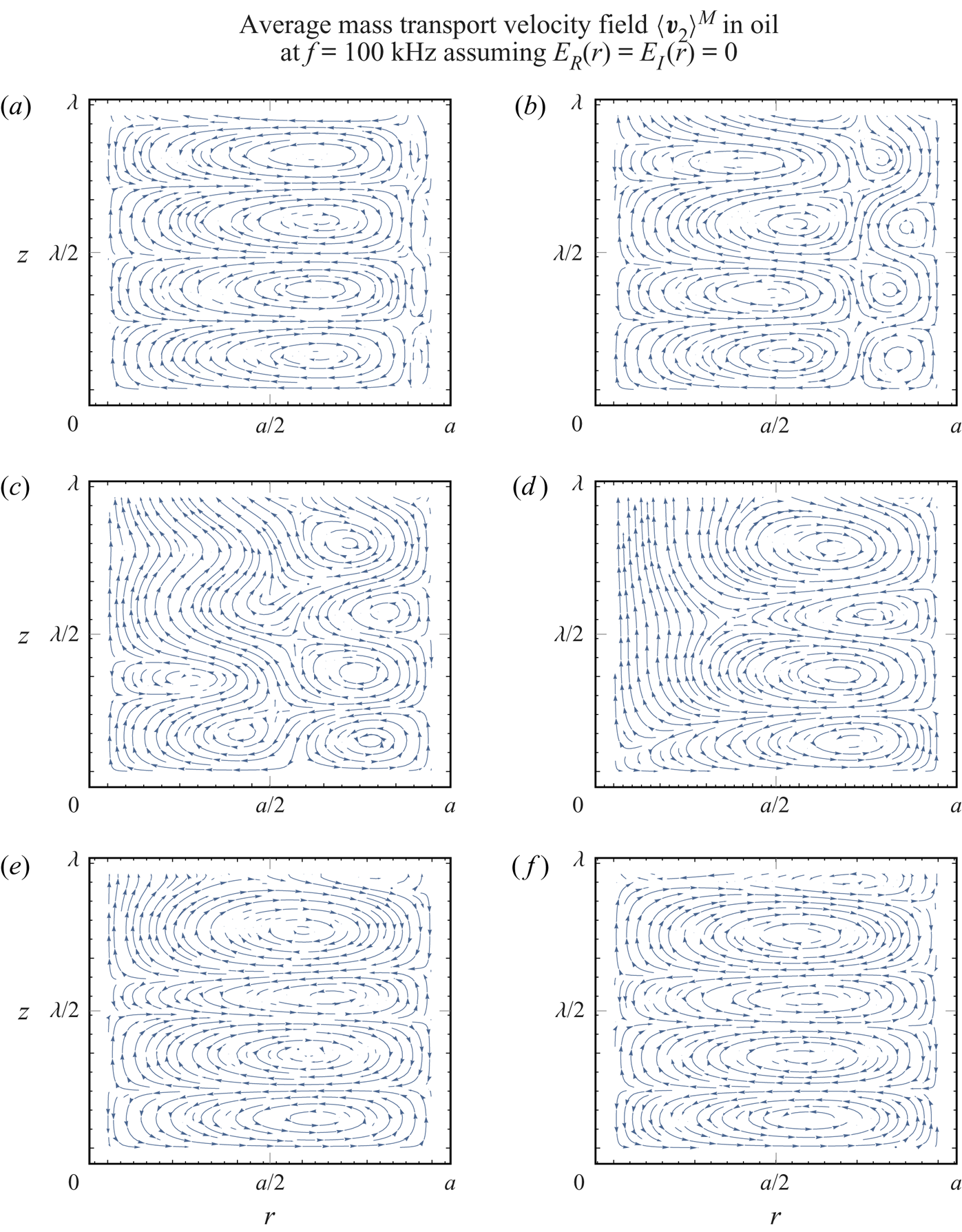
Figure 17. The average mass transport velocity patterns in oil, assuming  $E_{{R}}(r) = E_{{I}}(r) = 0$, for a tube radius of (a) $a=270\ {\mathrm {\mu }}\textrm {m}$ $(\varXi = 22.5)$, (b) $a=120\ {\mathrm {\mu }}\textrm {m}$ $(\varXi = 10)$, (c) $a=90\ {\mathrm {\mu }}\textrm {m}$ $(\varXi = 7.5)$, (d) $a=70\ {\mathrm {\mu }}\textrm {m}$ $(\varXi = 5.83)$, (e) $a=50\ {\mathrm {\mu }}\textrm {m}$ $(\varXi = 4.17)$ and (f) $a=40\ {\mathrm {\mu }}\textrm {m}$ $(\varXi = 3.33)$, for $f = 100\ \textrm {kHz}$. The corresponding acoustic wavelength is $\lambda = 14.45\ \textrm {mm}$, while the actual wavelength is $14.14\ \textrm {mm} \geqslant \lambda _{{R}} \geqslant 12.67\ \textrm {mm}$. The viscous boundary layer has a thickness of $\delta = 12\ {\mathrm {\mu }}\textrm {m}$. The first velocity node is at $z=0$, while the first velocity antinode appears at $z = \lambda _{{R}} / 4$. Arrows indicate the direction of the flow.
In figure 18, we analogously repeat the analysis of  $\varXi _{{S}}^{{M}}$ from figure 11. We observe that the transition from the Rayleigh-plus-Schlichting streaming to the Schlichting streaming occurs at lower value of $\varXi$ when the source terms $E_{{R}}(r)$ and $E_{{I}}(r)$ are neglected. Specifically, the critical normalized radius $\varXi _{{S}}^{{M}}$ is reduced from $6.2$ to $5.8$. Interestingly, this value corresponds to the Eulerian-streaming-velocity-based $\varXi _{{S}}$ of the incompressible streaming flow solution (figure 15).
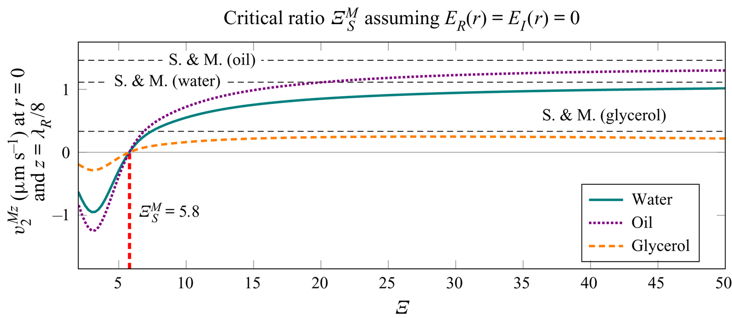
Figure 18. The  $z$-component of the average mass transport velocity, $v_2^{{M} z}$, assuming $E_{{R}}(r) = E_{{I}}(r) = 0$, at $r=0$ and $z=\lambda _{{R}} / 8$, depending on the normalized tube radius $\varXi = a / \delta$, for $f = 100\ \textrm {kHz}$ and $p_{{a}} = 100\ \textrm {kPa}$. The critical ratio $\varXi _{{S}}^{{M}}$ is defined as the value of $\varXi$ at which $v_2^{{M} z}$ changes direction. The velocity magnitudes (S. & M.) calculated with the model of Schuster & Matz (Reference Schuster and Matz1940) are given for reference (see (G2) in appendix G).
6. Conclusions
We derived an analytical solution for the motion of a viscous fluid at the first and at the second order in a tube of infinite length containing a pseudo-standing wave composed of two counterpropagating decaying travelling waves along the axis of the tube. The solution is valid for arbitrary thicknesses of the viscous boundary layer  $\delta$ relative to the radius of the tube $a$, and is not restricted by the acoustic wavelength $\lambda$. In addition, the applicability of our solution was demonstrated through analysis of several cases, with the help of numerical integration in Mathematica 12.0 (Wolfram Research, Inc., 2019), revealing the streaming patterns and their evolution with respect to the varying problem parameters. The Mathematica Notebook file with the implementations of all necessary expressions for evaluation of arbitrary streaming fields is available in the supplementary material. In our analysis, we observed two types of streaming vortices, namely Rayleigh streaming (fluid flow from the velocity node to the antinode near the axis of the tube) and the oppositely directed Schlichting streaming. The Rayleigh streaming is suppressed by the Schlichting streaming when the ratio of the tube radius to the thickness of the viscous boundary layer (i.e. $\varXi = a/\delta$) is below the critical value of $\varXi _{{S}}^{{M}}=6.2$, considering the average mass transport velocity, for $\varLambda = \lambda /a \gg 1$. If the Eulerian streaming velocity is considered, the transition occurs at $\varXi _{{S}} = 5.6$. The critical radii $\varXi _{{S}}^{{M}}$ and $\varXi _{{S}}$ at which the transitions between different streaming regimes occur are invariant with respect to the material parameters, as long as we are in the limit of $\varLambda \gg 1$. Similar behaviour was also predicted for a two-dimensional channel by Hamilton et al. (Reference Hamilton, Ilinskii and Zabolotskaya2003a), who evaluated $\varXi _{{S}}^{{M}}$ at $5.7$, but with the radius replaced by the half-width of their channel.
The vortices appear to be very distinct when a single vortex type, either Rayleigh or Schlichting, is dominant, e.g. figure 6(a,f). In the intermediate region, where  $\varXi$ is decreasing towards $\varXi _{{S}}$, we observe non-periodic behaviour along the $z$-axis (e.g. figure 6c,d), which can be attributed to the decaying nature of the pseudo-standing wave. The amplitude of the acoustic streaming was found to be dependent on the normalized radius $\varXi$. The amplitude is lowest when $\varXi$ corresponds to the regime where neither Rayleigh nor Schlichting streaming dominates (i.e. $20 \gtrsim \varXi > \varXi _{{S}}$). However, for $\varXi \gtrsim 20$, the streaming velocity magnitude at the centre of the tube matches relatively well to the solution of Schuster & Matz (Reference Schuster and Matz1940).
When  $\varXi > \varXi _{{S}}$, decreasing $\varLambda$ can result in a transition from Rayleigh streaming vortices to a large-scale Eckart-like streaming (figure 13). The critical ratio $\varLambda$ at which this transition occurs was evaluated for the case of glycerol at a constant $\varXi$ of $22.5$, and stands at $\varLambda _{{E}}^{{M}} = 3.5$ for the average mass transport velocity, and at $\varXi _{{E}} = 3.1$ for the Eulerian streaming velocity (figure 12).
The investigation of the contribution of the compressibility of the streaming flow indicated that the resulting Eulerian streaming velocity patterns (figure 15) better resemble the average mass transport velocity patterns of the compressible solution (figure 6) than the patterns of the compressible Eulerian streaming velocity (figure 7). Compressibility appears to decrease the critical ratio  $\varXi _{{S}}$, since the incompressible solution yields $\varXi _{{S}} = 5.8$, whereas the compressible solution yields $\varXi _{{S}} = 5.6$.
The analysis of the effects of the individual streaming source terms revealed that all terms originating from the spatial variation of the Reynolds stress have to be considered to correctly predict the streaming patterns. Neglecting the commonly-neglected the source term, namely  $\left \langle \boldsymbol {v}_1 \boldsymbol {\nabla } \boldsymbol {\cdot } \boldsymbol {v}_1 \right \rangle = 0$ (for example, Rayleigh (Reference Rayleigh1884), Schlichting (Reference Schlichting1932), Lighthill (Reference Lighthill1978) and Doinikov et al. (Reference Doinikov, Thibault and Marmottant2017) neglect this term), leads to the decrease of the critical ratio $\varXi _{{S}}^{{M}}$ (from $6.2$ to $5.8$), but still offers a good approximation. Interestingly, the average-mass-transport-velocity-based $\varXi _{{S}}^{{M}}=5.8$ of the solution with partially neglected source terms matches the Eulerian-streaming-velocity-based $\varXi _{{S}}$ of the incompressible solution, and the corresponding streaming patterns match as well.
Supplementary material
Supplementary material is available at https://doi.org/10.1017/jfm.2020.1046.
Acknowledgements
We would like to express our gratitude to A. A. Doinikov for helpful discussions on the topics involving acoustic streaming that served as an inspiration for the present work.
Declaration of interests
The authors report no conflict of interest.
Appendix A
This appendix contains the results for air (material properties are given in table 1). The wavenumber in air for  $f = 100\ \textrm {kHz}$ and $f = 1\ \textrm {MHz}$ is given in figure 19. The first-order pressure for air at different tube radii is given in figure 20. In figure 21, it is shown that the discovered critical ratios $\varXi _{{S}} = 5.6$ and $\varXi _{{S}}^{{M}} = 6.2$, in the limit of $\lambda \gg a$, also hold for air.
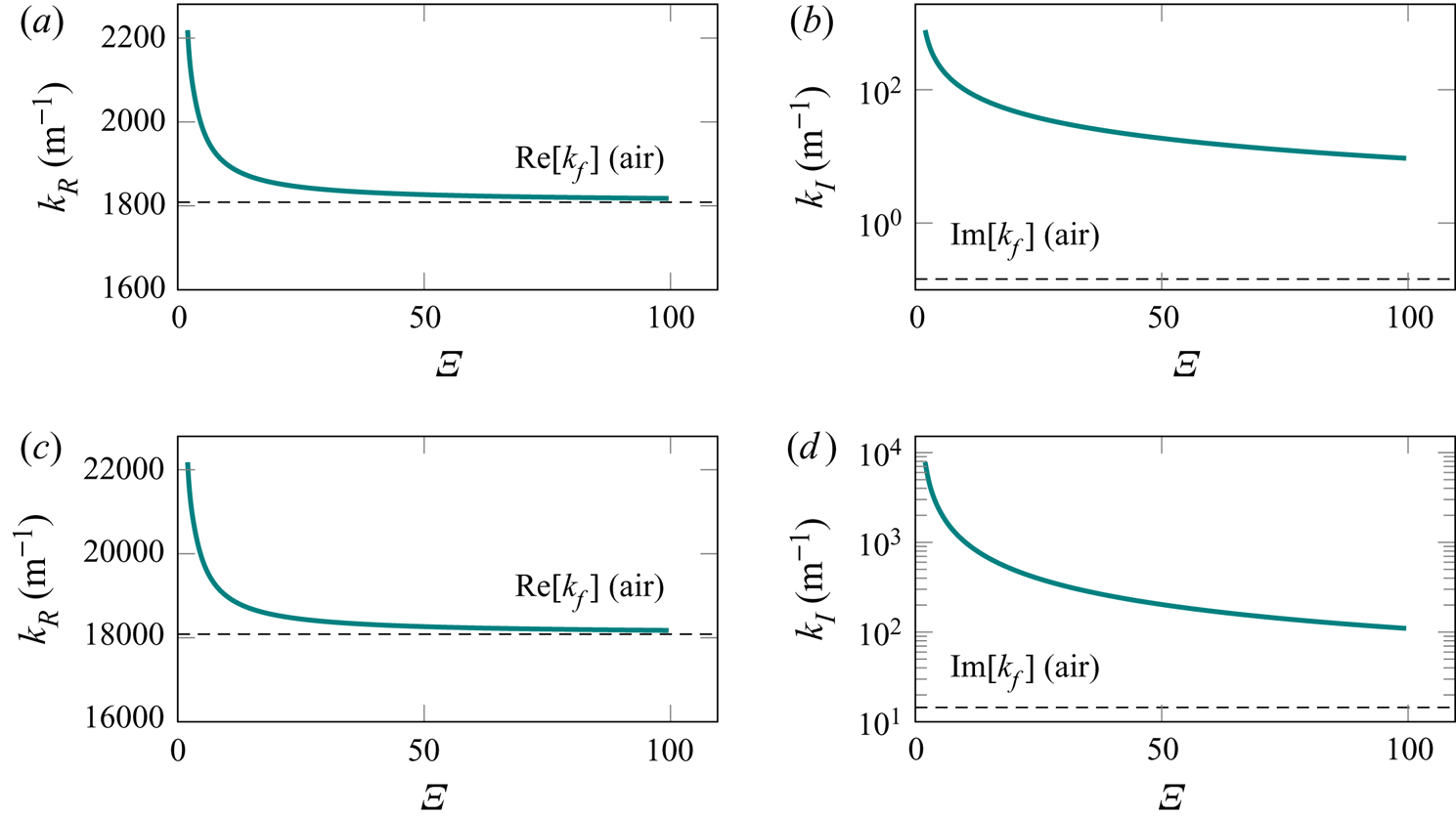
Figure 19. The real and imaginary parts of the wavenumber in air according to (3.31) and (3.32), respectively: (a)  $k_R$ at $f = 100\ \textrm {MHz}$; (b) $k_I$ at $f = 100\ \textrm {kHz}$; (c) $k_R$ at $f = 1\ \textrm {MHz}$; (d) $k_I$ at $f = 1\ \textrm {MHz}$. The dimensionless ratio $\varXi = a / \delta$ represents the varying tube radius relative to the viscous boundary layer thickness. The real and imaginary parts of the wavenumber in an unbounded fluid domain $k_{{f}}$ are plotted for reference.
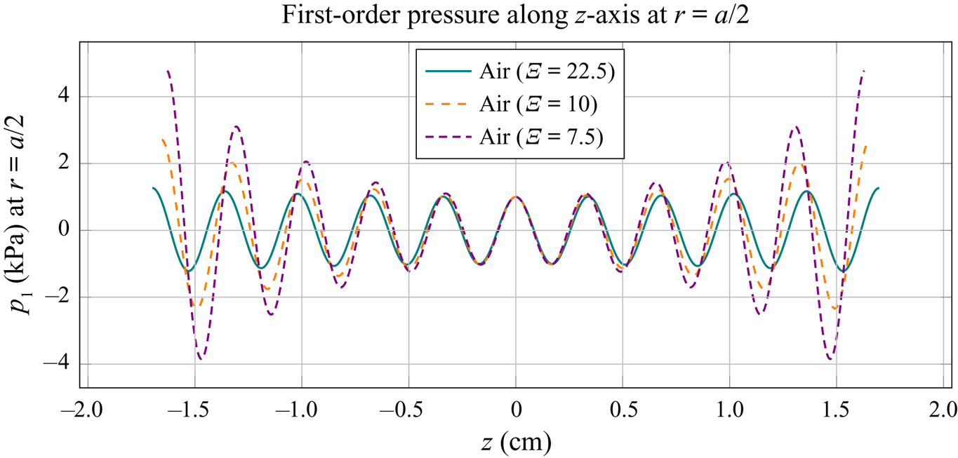
Figure 20. The first-order pressure in air along the  $z$-axis, at $r=a/2$, for $f = 100\ \textrm {kHz}$ and $p_{{a}} = 1\ \textrm {kPa}$. The dimensionless ratio $\varXi = a / \delta$ represents the varying tube radius relative to the viscous boundary layer thickness of $\delta = 7.13\ {\mathrm {\mu }}\textrm {m}$. For each radius of the tube, we plot the pressure in the range of $- 5 \lambda _{{R}} < z < 5 \lambda _{{R}}$, with $\lambda _{{R}} = 2 {\rm \pi}/ k_{{R}}$.
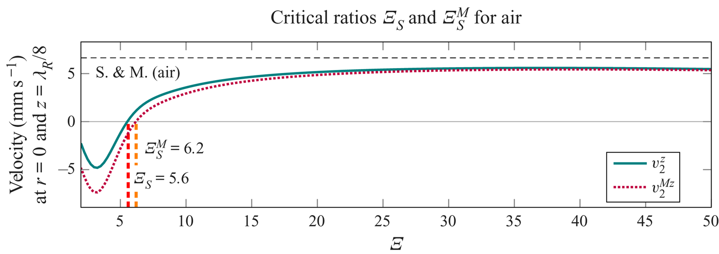
Figure 21. The  $z$-components of the Eulerian streaming velocity, $v_2^{z}$, and of the average mass transport velocity, $v_2^{{M} z}$, in air, at $r = 0$ and $z = \lambda _{{R}} / 8$, depending on the normalized tube radius $\varXi = a / \delta$, for $f = 100\ \textrm {kHz}$ and $p_{{a}} = 1\ \textrm {kPa}$. The critical ratios $\varXi _{{S}}$ and $\varXi _{{S}}^{{M}}$ are defined as the values of $\varXi$ at which $v_2^z$ and $v_2^{{M} z}$, respectively, change direction. The velocity magnitude (S. & M.) calculated with the model of Schuster & Matz (Reference Schuster and Matz1940) is given for reference (see (G2) in appendix G).
Appendix B
Here we analyse the convergence of different parts of the solution with respect to the summation limit  $i_{{max}}$, at which the infinite summations in (4.26), (4.27), (4.56), (4.57), (E1) and (E2) are truncated. In figure 22, the convergence of the $z$-component of the Eulerian streaming velocity, $v_2^z$, is evaluated at different positions (figure 22e–h), in addition to the convergence of the constants $C_1$ and $C_3$ (figure 22a–d). The exemplary convergence study in figure 22 corresponds to the case from figure 6(f), with oil at $100\ \textrm {kHz}$, $p_{{a}} = 100\ \textrm {kPa}$, $a=40\ \mathrm {\mu }\textrm {m}$ and $\varXi =3.33$. The solution appears to be converged for $i_{{max}} \gtrsim 100$. However, it appears from figure 22(e) that $v_2^z$ converges slower when the point of evaluation is closer to $r=a$. This has been confirmed by further analysis of convergence at higher $\varXi$, where the sufficient $i_{{max}}$ was evaluated to be much higher. For the purposes of our study, using $i_{{max}}$ of up to $200$ was sufficient.
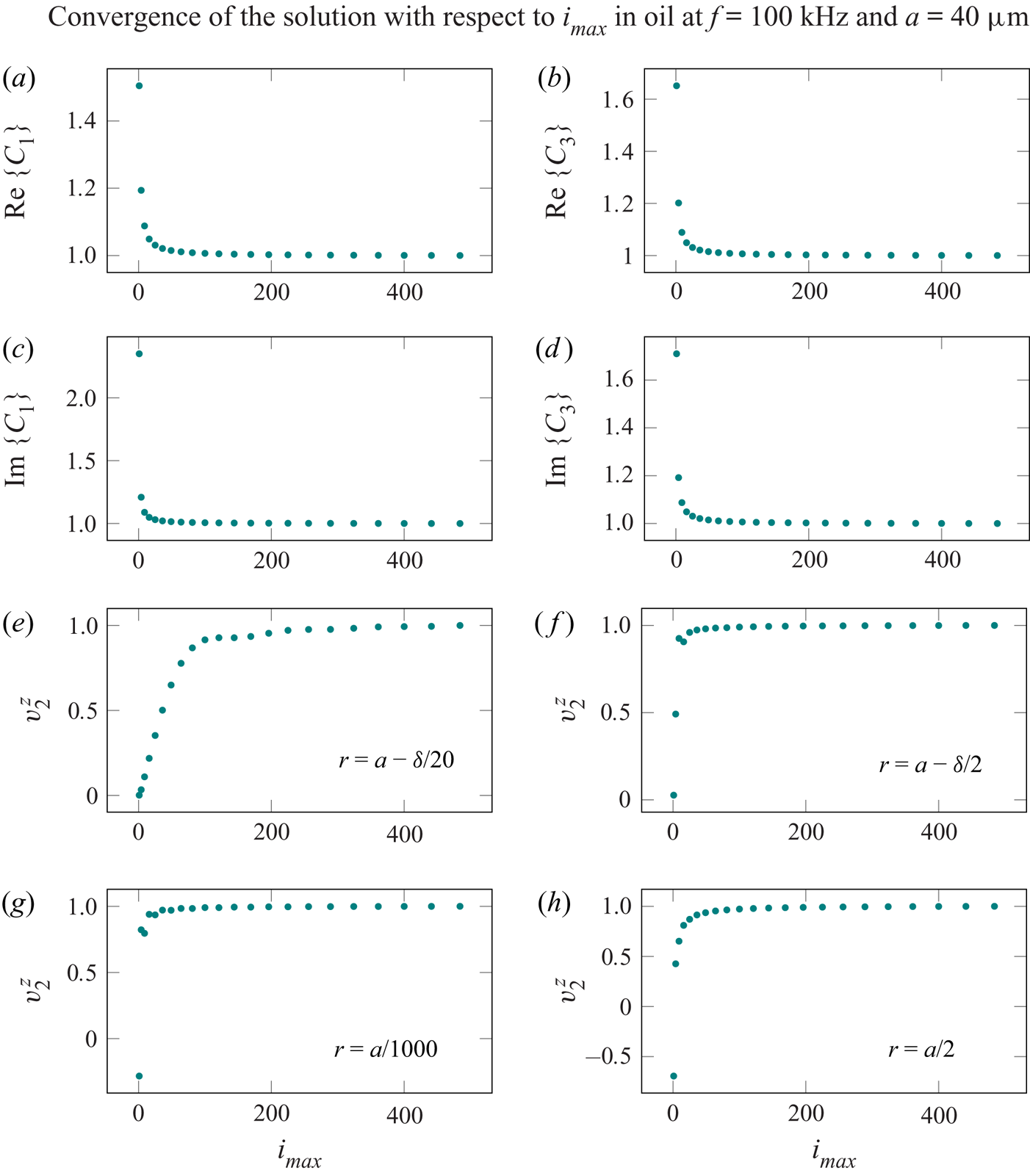
Figure 22. Analysis of the convergence of different parts of the solution with respect to the summation index  $i_{{max}}$, at which the infinite summations in (4.26), (4.27), (4.56), (4.57), (E1) and (E2) are truncated. Panels (a–d) show the convergence of the constants $C_1$ and $C_3$, and panels (e–h) the convergence of the $z$-component of the Eulerian streaming velocity, $v_2^z$, evaluated at different positions along $a/1000 \leq r \leq a-\delta /20$. The values of each quantity are normalized with the value at the maximal $i_{{max}}$ in the convergence study. (a) Re $\{C_1\}$. (b) Re $\{C_3\}$. (c) Im $\{C_1\}$. (d) Im $\{C_3\}$. (e–h) $v^z_2$ at the r-values indicated.
Appendix C
Here we give the expressions for the functions  $R_{{R}}(r)$, $E_{{R}}(r)$, $R_{{I}}(r)$ and $E_{{I}}(r)$:
 \begin{gather} R_{{R}}(r) = \frac{- A_1}{r |k|^2 |J_1 (q_{{v}} a)|^2} \left( r k q_{{f}} A_1^* \left[ J_0 (q_{{f}} r) J_1 (q_{{v}} a) k^2 + q_{{f}} q_{{v}} J_0 (q_{{v}} r) J_1 (q_{{f}} a) \right]^* \right. \nonumber\\ \left[ |k|^2 J_1 (q_{{v}} a) J_1 (q_{{f}} r) - J_1 (q_{{f}} a) \left( 2 k k_{{R}} + q_{{v}}^2 \right) J_1 (q_{{v}} r) \right] \nonumber\\ - r k \left[ k^2 J_1 (q_{{v}} a) J_0 (q_{{f}} r) + q_{{f}} q_{{v}} J_1 (q_{{f}} a) J_0 (q_{{v}} r) \right] \nonumber\\ \left[ q_{{f}} A_1 \left( J_1 (q_{{v}} a) J_1 (q_{{f}} r) k^2 + q_{{v}}^2 J_1 (q_{{f}} a) J_1 (q_{{v}} r) \right) \right]^* \nonumber\\ + q_{{f}} k^* \left\{ k_{{v}}^2 J_1 (q_{{f}} a) \left( J_1 (q_{{v}} r) - r q_{{v}} J_0 (q_{{v}} r) \right) \right. \nonumber\\ \left( q_{{f}} A_1 \left[ J_1 (q_{{v}} a) J_1 (q_{{f}} r) - J_1 (q_{{f}} a) J_1 (q_{{v}} r) \right] \right)^* \nonumber\\ \left( k^2 J_1 (q_{{v}} a) J_1 (q_{{f}} r) + q_{{v}}^2 J_1 (q_{{f}} a) J_1 (q_{{v}} r) \right) \nonumber\\ \left( q_{{f}} A_1 \left[ r q_{{v}} J_0 (q_{{v}} r) J_1 (q_{{f}} a) - J_1 (q_{{v}} r) J_1 (q_{{f}} a) + J_1 (q_{{v}} a) \left( J_1 (q_{{f}} r) - r q_{{f}} J_0 (q_{{f}} r) \right) \right] \right)^* \nonumber\\ + k \left( - r q_{{v}} J_1 (q_{{f}} a) J_0 (q_{{v}} r) + J_1 (q_{{f}} a) J_1 (q_{{v}} r) + J_1 (q_{{v}} a) \left[ r q_{{f}} J_0 (q_{{f}} r) - J_1 (q_{{f}} r) \right] \right) \nonumber\\ \left. \left. \left( k q_{{f}} A_1 \left[ J_1 (q_{{v}} a) J_1 (q_{{f}} r) - J_1 (q_{{f}} a) J_1 (q_{{v}} r) \right] \right)^* \right\} \right) , \end{gather}
 \begin{gather} R_{{I}}(r) = \frac{- A_1}{r |k|^2 |J_1 (q_{{v}} a)|^2} \left( r k q_{{f}} A_1^* \left[ J_0 (q_{{f}} r) J_1 (q_{{v}} a) k^2 + q_{{f}} q_{{v}} J_0 (q_{{v}} r) J_1 (q_{{f}} a) \right]^* \right. \nonumber\\ \left[ |k|^2 J_1 (q_{{v}} a) J_1 (q_{{f}} r) + J_1 (q_{{f}} a) \left( 2 \mathrm{i} k k_{{I}} + q_{{v}}^2 \right) J_1 (q_{{v}} r) \right] \nonumber\\ + r k \left[ k^2 J_1 (q_{{v}} a) J_0 (q_{{f}} r) + q_{{f}} q_{{v}} J_1 (q_{{f}} a) J_0 (q_{{v}} r) \right] \nonumber\\ \left[ q_{{f}} A_1 \left( J_1 (q_{{v}} a) J_1 (q_{{f}} r) k^2 + q_{{v}}^2 J_1 (q_{{f}} a) J_1 (q_{{v}} r) \right) \right]^* \nonumber\\ + q_{{f}} k^* \left\{ k_{{v}}^2 J_1 (q_{{f}} a) \left( J_1 (q_{{v}} r) - r q_{{v}} J_0 (q_{{v}} r) \right) \right. \nonumber\\ \left( q_{{f}} A_1 \left[ J_1 (q_{{v}} a) J_1 (q_{{f}} r) - J_1 (q_{{f}} a) J_1 (q_{{v}} r) \right] \right)^* \nonumber\\ \left( k^2 J_1 (q_{{v}} a) J_1 (q_{{f}} r) + q_{{v}}^2 J_1 (q_{{f}} a) J_1 (q_{{v}} r) \right) \nonumber\\ \left( q_{{f}} A_1 \left[ r q_{{v}} J_0 (q_{{v}} r) J_1 (q_{{f}} a) - J_1 (q_{{v}} r) J_1 (q_{{f}} a) + J_1 (q_{{v}} a) \left( J_1 (q_{{f}} r) - r q_{{f}} J_0 (q_{{f}} r) \right) \right] \right)^*\nonumber\\ + k \left( r q_{{v}} J_1 (q_{{f}} a) J_0 (q_{{v}} r) - J_1 (q_{{f}} a) J_1 (q_{{v}} r) + J_1 (q_{{v}} a) \left[ - r q_{{f}} J_0 (q_{{f}} r) + J_1 (q_{{f}} r) \right] \right) \nonumber\\ \left. \left. \left( k q_{{f}} A_1 \left[ J_1 (q_{{v}} a) J_1 (q_{{f}} r) - J_1 (q_{{f}} a) J_1 (q_{{v}} r) \right] \right)^* \right\} \right),\end{gather}
 \begin{gather} E_{{R}}(r) = \frac{A_1}{r^2 |k|^2 |J_1 (q_{{v}} a)|^2} \left( k^* \left\{ \left( k^2 J_1 (q_{{v}} a) J_0 (q_{{f}} r) \left[ 1 - r^2 k_{{f}}^2 \right] + r k^2 q_{{f}} J_1 (q_{{v}} a) J_1 (q_{{f}} r) \right. \right. \right. \nonumber\\ \left.+ r q_{{f}} q_{{v}}^2 J_1 (q_{{f}} a) J_1 (q_{{v}} r) + q_{{f}} q_{{v}} J_1 (q_{{f}} a) J_0 (q_{{v}} r) \right) \nonumber\\ \left( A_1 q_{{f}} \left[ J_1 (q_{{v}} a) J_1 (q_{{f}} r) - J_1 (q_{{f}} a) J_1 (q_{{v}} r) \right] \right)^* - r^2 k k_{{f}} J_1 (q_{{v}} a) J_0 (q_{{f}} r) \nonumber\\ \left( A_1 k q_{{f}} \left[ J_1 (q_{{v}} a) J_1 (q_{{f}} r) - J_1 (q_{{f}} a) J_1 (q_{{v}} r) \right] \right)^* \nonumber\\ + \left( k^2 J_1 (q_{{v}} a) J_0 (q_{{f}} r) + q_{{v}} q_{{f}} J_1 (q_{{f}} a) J_0 (q_{{v}} r) \right) \nonumber\\ \left. \left( A_1 q_{{f}} \left[ r q_{{v}} J_0 (q_{{v}} r) J_1 (q_{{f}} a) - J_1 (q_{{v}} r) J_1 (q_{{f}} a) + J_1 (q_{{v}} a) \left( J_1 (q_{{f}} r) - r q_{{f}} J_0 (q_{{f}} r) \right) \right] \right)^* \right\} \nonumber\\ + r k \left[ r k_{{f}}^2 J_1 (q_{{v}} a) J_0 (q_{{f}} r) - q_{{f}} J_1 (q_{{v}} a) J_1 (q_{{f}} r) + q_{{f}} J_1 (q_{{f}} a) J_1 (q_{{v}} r) \right] \nonumber\\ \left[ A_1 q_{{f}} \left( k^2 J_1 (q_{{v}} a) J_1 (q_{{f}} r) + q_{{v}}^2 J_1 (q_{{f}} a) J_1 (q_{{v}} r) \right) \right]^* \nonumber\\ + r k q_{{f}} \left[ J_1 (q_{{v}} a) \left( r k_{{f}}^2 J_1 (q_{{f}} r) - q_{{f}} J_2 (q_{{f}} r) \right) + q_{{v}} J_1 (q_{{f}} a) J_2 (q_{{v}} r) \right] \nonumber\\ \left. \left[ A_1 k^2 J_0 (q_{{f}} r) J_1 (q_{{v}} a) + A_1 q_{{f}} q_{{v}} J_0 (q_{{v}} r) J_1 (q_{{f}} r) \right]^* \right) , \end{gather}
 \begin{gather} E_{{I}}(r) = \frac{A_1}{r^2 |k|^2 |J_1 (q_{{v}} a)|^2} \left( k^* \left\{ \left( k^2 J_1 (q_{{v}} a) J_0 (q_{{f}} r) \left[ 1 - r^2 k_{{f}}^2 \right] + r k^2 q_{{f}} J_1 (q_{{v}} a) J_1 (q_{{f}} r) \right. \right. \right. \nonumber\\ \left.+ r q_{{f}} q_{{v}}^2 J_1 (q_{{f}} a) J_1 (q_{{v}} r) + q_{{f}} q_{{v}} J_1 (q_{{f}} a) J_0 (q_{{v}} r) \right) \nonumber\\ \left( A_1 q_{{f}} \left[ J_1 (q_{{v}} a) J_1 (q_{{f}} r) - J_1 (q_{{f}} a) J_1 (q_{{v}} r) \right] \right)^* + r^2 k k_{{f}} J_1 (q_{{v}} a) J_0 (q_{{f}} r) \nonumber\\ \left( A_1 k q_{{f}} \left[ J_1 (q_{{v}} a) J_1 (q_{{f}} r) - J_1 (q_{{f}} a) J_1 (q_{{v}} r) \right] \right)^* \nonumber\\ + \left( k^2 J_1 (q_{{v}} a) J_0 (q_{{f}} r) + q_{{v}} q_{{f}} J_1 (q_{{f}} a) J_0 (q_{{v}} r) \right) \nonumber\\ \left. \left( A_1 q_{{f}} \left[ r q_{{v}} J_0 (q_{{v}} r) J_1 (q_{{f}} a) - J_1 (q_{{v}} r) J_1 (q_{{f}} a) + J_1 (q_{{v}} a) \left( J_1 (q_{{f}} r) - r q_{{f}} J_0 (q_{{f}} r) \right) \right] \right)^* \right\} \nonumber\\ - r k \left[ r k_{{f}}^2 J_1 (q_{{v}} a) J_0 (q_{{f}} r) - q_{{f}} J_1 (q_{{v}} a) J_1 (q_{{f}} r) + q_{{f}} J_1 (q_{{f}} a) J_1 (q_{{v}} r) \right] \nonumber\\ \left[ A_1 q_{{f}} \left( k^2 J_1 (q_{{v}} a) J_1 (q_{{f}} r) + q_{{v}}^2 J_1 (q_{{f}} a) J_1 (q_{{v}} r) \right) \right]^* \nonumber\\ - r k q_{{f}} \left[ J_1 (q_{{v}} a) \left( r k_{{f}}^2 J_1 (q_{{f}} r) - q_{{f}} J_2 (q_{{f}} r) \right) + q_{{v}} J_1 (q_{{f}} a) J_2 (q_{{v}} r) \right] \nonumber\\ \left. \left[ A_1 k^2 J_0 (q_{{f}} r) J_1 (q_{{v}} a) + A_1 q_{{f}} q_{{v}} J_0 (q_{{v}} r) J_1 (q_{{f}} r) \right]^* \right) . \end{gather}
Appendix D
The source terms connected to the scalar velocity potential  $\varphi _2$ are given below:
 \begin{align} M_{{R}} (r) &= - A_1 k_{{f}}^2 J_0 (q_{{f}}^{*} r) J_0 (q_{{f}} r) + A_1 q_{{f}}^{*} q_{{f}} J_1 (q_{{f}}^{*} r) J_1 (q_{{f}} r) \nonumber\\ &\quad + \mathrm{i} B_1 k q_{{f}}^{*} J_1 (q_{{f}}^{*} r) J_1 (q_{{v}} r) - A_1 k^{*} k J_0 (q_{{f}}^{*} r) J_0 (q_{{f}} r) \nonumber\\ &\quad + \mathrm{i} B_1 k^{*} q_{{v}} J_0 (q_{{f}}^{*} r) J_0 (q_{{v}} r), \end{align}
 \begin{align} M_{{I}} (r) &= - A_1 k_{{f}}^2 J_0 (q_{{f}}^{*} r) J_0 (q_{{f}} r) + A_1 q_{{f}}^{*} q_{{f}} J_1 (q_{{f}}^{*} r) J_1 (q_{{f}} r) \nonumber\\ &\quad + \mathrm{i} B_1 k q_{{f}}^{*} J_1 (q_{{f}}^{*} r) J_1 (q_{{v}} r) + A_1 k^{*} k J_0 (q_{{f}}^{*} r) J_0 (q_{{f}} r) \nonumber\\ &\quad - \mathrm{i} B_1 k^{*} q_{{v}} J_0 (q_{{f}}^{*} r) J_0 (q_{{v}} r). \end{align}
Appendix E
The differentiation of (4.26) with respect to  $r$ leads to
 \begin{align} \frac{\mathrm{d} S_{{R}}(r)}{\mathrm{d} r} &= \frac{2}{a^2} \sum_{i=1}^{\infty} \frac{\frac{1}{r} J_1 ( \xi_i r ) - \xi_i J_2 (\xi_i r)}{[J_2 ( \xi_i a )]^2 \left( \xi_i^2 + 4 k_{{R}}^2 \right)^2} \left[\vphantom{\left( \xi_i^2 J_2 ( \xi_i a ) - 8 k_{{R}}^2 \right)} \bar{R}_{{R}}(\xi_{i}) + \bar{E}_{{R}}(\xi_{i}) \right.\nonumber\\ &\quad \left. - a \xi_i C_1 J_2 ( \xi_i a ) + a \xi_i C_2 \left( \xi_i^2 J_2 ( \xi_i a ) - 8 k_{{R}}^2 \right) \right], \end{align}
and similarly for (4.27),
 \begin{align} \frac{\mathrm{d} S_{{I}}(r)}{\mathrm{d} r} &= \frac{2}{a^2} \sum_{i=1}^{\infty} \frac{\dfrac{1}{r} J_1 ( \xi_i r ) - \xi_i J_2 (\xi_i r)}{[J_2 ( \xi_i a )]^2 \left( \xi_i^2 - 4 k_{{I}}^2 \right)^2} \left[\vphantom{\left( \xi_i^2 J_2 ( \xi_i a ) - 8 k_{{R}}^2 \right)} \bar{R}_{{I}}(\xi_{i}) + \bar{E}_{{I}}(\xi_{i})\right. \nonumber\\ &\quad \left. - a \xi_i C_3 J_2 ( \xi_i a ) + a \xi_i C_4 \left( \xi_i^2 J_2 ( \xi_i a ) + 8 k_{{I}}^2 \right) \right]. \end{align}
 The differentiation of (4.41) with respect to  $r$ leads to
 \begin{align} \frac{\mathrm{d} U_{{R}}(r)}{\mathrm{d} r} &= {\rm \pi}\mathrm{i} k_{{R}} J_1 (2 \mathrm{i} k_{{R}} r) \int_0^r x M_{{R}} (x) Y_0 (-2 \mathrm{i} k_{{R}} x) \, \mathrm{d}x \nonumber\\ &\quad + {\rm \pi}\mathrm{i} k_{{R}} Y_1 (-2 \mathrm{i} k_{{R}} r) \int_0^r x M_{{R}} (x) J_0 (2 \mathrm{i} k_{{R}} x) \, \mathrm{d}x - 2 \mathrm{i} k_{{R}} C_5 J_1 (2 \mathrm{i} k_{{R}} r) , \end{align}
and similarly for (4.42),
 \begin{align} \frac{\mathrm{d} U_{{I}}(r)}{\mathrm{d} r} &= {\rm \pi}k_{{I}} J_1 (2 k_{{I}} r) \int_0^r x M_{{I}} (x) Y_0 (2 k_{{I}} x) \, \mathrm{d}x \nonumber\\ &\quad - {\rm \pi}k_{{I}} Y_1 (2 k_{{I}} r) \int_0^r x M_{{I}} (x) J_0 (2 k_{{I}} x) \, \mathrm{d}x - 2 k_{{I}} C_7 J_1 (2 k_{{I}} r) . \end{align}
Appendix F
The Stokes drift is given by
 \begin{gather} \boldsymbol{v}_{{SD}} = \frac{2}{\omega} \mathrm{Re} \left\{ \left[ \left( - \mathrm{i} q_{{f}} A_1 J_0 (q_{{f}} r) + k B_1 J_1 (q_{{v}} r) \right) \left( - q_{{f}}^2 A_1 J_0 (q_{{f}} r) + \frac{1}{r} q_{{f}} A_1 J_1 (q_{{f}} r)\right.\right.\right. \nonumber\\ \left.+ \frac{1}{r} \mathrm{i} k B_1 J_1 (q_{{v}} r) - \mathrm{i} k q_{{v}} B_1 J_0 (q_{{v}} r) \right)^{*} \left( \cos^2 (k_{{R}} z) + \sinh^2 (k_{{I}} z) \right) \nonumber\\ + \mathrm{i} \left( -k A_1 J_0 (q_{{f}} r) + \mathrm{i} q_{{v}} B_1 J_0 (q_{{v}} r) \right) \left( k q_{{f}} A_1 J_1 (q_{{f}} r) + \mathrm{i} k^2 B_1 J_1 (q_{{v}} r) \right)^{*} \nonumber\\ \left.\left( \sin^2 (k_{{R}} z) + \sinh^2 (k_{{I}} z) \right) \vphantom{\frac{1}{r}}\right] \boldsymbol{e}_{r}\nonumber\\ + \frac{1}{2} \left[ \left( - \mathrm{i} q_{{f}} A_1 J_1 (q_{{f}} r) + k B_1 J_1 (q_{{v}} r) \right) \left( k q_{{f}} A_1 J_1 (q_{{f}} r) - \mathrm{i} q_{{v}}^2 B_1 J_1 (q_{{v}} r) \right)^{*}\right. \nonumber\\ \left( \sin (2 k_{{R}} z) - \mathrm{i} \sinh (2 k_{{I}} z) \right) \nonumber\\ + \mathrm{i} \left( -k A_1 J_0 (q_{{f}} r) + \mathrm{i} q_{{v}} B_1 J_0 (q_{{v}} r) \right) \left( - k^2 A_1 J_0 (q_{{f}} r) + \mathrm{i} k q_{{v}} B_1 J_0 (q_{{v}} r) \right)^{*} \nonumber\\ \left.\left.\left( \sin (2 k_{{R}} z) + \mathrm{i} \sinh (2 k_{{I}} z) \right) \vphantom{\frac{1}{q}}\right] \boldsymbol{e}_z \vphantom{\frac{1}{q}}\right\} . \end{gather}
Appendix G
Schuster & Matz (Reference Schuster and Matz1940) calculated the streaming velocity outside the viscous boundary layer, for a non-decaying wave along  $z$-axis, as
 \begin{align} \left\langle \boldsymbol{v}_2 \right\rangle^{{S}} &= - \frac{3}{8} \frac{p_{{a}}^2 \omega}{c_{{f}}^4 \rho_0^2} r \cos \left( \frac{2 \omega}{c_{{f}}} \left( z - \frac{\lambda}{4}\right) \right) \left\{1 - \frac{r^2}{a^2} \right\} \boldsymbol{e}_r \nonumber\\ &\quad - \frac{3}{8} \frac{p_{{a}}^2}{c_{{f}}^3 \rho_0^2} \sin \left( \frac{2 \omega}{c_{{f}}} \left( z - \frac{\lambda}{4}\right) \right) \left\{1 - \frac{2 r^2}{a^2} \right\} \boldsymbol{e}_z , \end{align}
where we have shifted the solution along  $z$-axis by $\lambda /4$ to match the position of the velocity node to $z=0$, as assumed in our formulation.
Schuster & Matz (Reference Schuster and Matz1940) also assume that  $\lambda _{{R}} = \lambda$, and the simplified expression for the velocity magnitude at $z=\lambda / 8$ and $r=0$ is given as
 \begin{equation} v_2^{{S} z} = \frac{3 p_{{a}}^2}{8 c_{{f}}^3 \rho_0^2}. \end{equation}


 Open access