


1. Introduction
Many buoyancy sources that occur in nature and the built environment are vertically distributed. Examples include a wall exposed to sunlight, a wall separating a room on fire from one at risk, a panel heater in a room and a vertical submerged ice wall of a glacier (Heiselberg & Sandberg Reference Heiselberg and Sandberg1990; Linden Reference Linden1999; Kerr & McConnochie Reference Kerr and McConnochie2015). The wall plume that develops adjacent to such a plane source, also referred to as a natural convection boundary layer, has been investigated extensively for an infinite wall in unbounded environments (George Jr. & Capp Reference George and Capp1979; Tsuji & Nagano Reference Tsuji and Nagano1989; McBain, Armfield & Desrayaud Reference McBain, Armfield and Desrayaud2007; Abedin, Tsuji & Hattori Reference Abedin, Tsuji and Hattori2009). These studies primarily focus on the details of the flow within the wall plume. Motivated by the spread of airborne contaminants, such as a virus from a common cold or influenza, Loganathan & Hunt (Reference Loganathan and Hunt2019) examine the flow induced in the ambient by a turbulent wall plume and develop an analytical solution that shows clearly delineated regions of accelerating and decelerating flow. Herein, we develop a closed-form solution for the complex pattern of stratified flow induced by a turbulent wall plume in a ventilated room, sharing the same motivation to enhance our understanding of airflow and contaminant movement in naturally ventilated rooms.
Turbulent wall plumes have also been intensively studied in confined spaces such as in a box in which the vertical plane source covers an entire internal wall of area  $H\times L$, with $H$ denoting the box height. This situation has clear practical applications, for example to the heating of a room. As a successor of the original ‘emptying–filling-box’ model proposed by Linden, Lane-Serff & Smeed (Reference Linden, Lane-Serff and Smeed1990), who considered a vertical line source extending from floor to ceiling in a ventilated container, Cooper & Hunt (Reference Cooper and Hunt2010) studied both sealed and ventilated boxes with a vertical plane source. By extending the ‘filling-box’ theory of Baines & Turner (Reference Baines and Turner1969), they found that in a sealed box, both the transient and asymptotic flow features, such as the descent of the ‘first front’ and uniform heating at large time, were qualitatively similar to those produced by a localised source on the base. In a ventilated box, with openings at the base (of area per unit length $a_l$) and top (of area per unit length $a_u$), however, multiple layers could form due to the continuous supply of buoyancy over the whole box height. By assuming that these layers have the same depth, $h$, the number of interfaces $n$ was acquired in Cooper & Hunt (Reference Cooper and Hunt2010) by solving
 \begin{equation} \frac{5}{4}\left(\frac{4}{3}\right)^3\left(\frac{A}{\alpha H}\right)^2=\frac{1}{n(n+1)^3}, \end{equation}
where the effective area (per unit length) of the box openings is
 \begin{equation} A=2^{{1}/{2}}c_uc_la_ua_l[(c_ua_u)^2+(c_la_l)^2]^{-{1}/{2}} \end{equation}
and  $\alpha$ denotes the entrainment coefficient of the wall plume. In (1.2), the dimensionless coefficients $c_u$ and $c_l$ account for the pressure loss at the upper and lower openings, respectively. The buoyancy jump across each density interface was then determined by calculating the increase of buoyancy along the wall plume within a layer over the depth $h$. Caudwell, Flór & Negretti (Reference Caudwell, Flór and Negretti2016) considered the case of a thermally heated wall in a sealed box, extending the constant-buoyancy-flux wall-plume analysis of Cooper & Hunt (Reference Cooper and Hunt2010) to a wall of constant temperature. Beyond this knowledge of the stratification and of the associated rate of buoyancy-driven fluid exchange through the openings $q_0$
$q_0$  $(\mathrm {m}^3\ \mathrm {s}^{-1})$, little else was previously known about the flow in the box, including the velocity field and streamline pattern induced by the wall plume within the individual layers.
With the boundary conditions being acquired from the entrainment rate at the plume perimeter, Hunt & Dyke (unpublished observations) deduced a closed-form solution for the potential flow induced in a ventilated box, with openings at top and base, by a horizontal line source of buoyancy located on its base. Their solution approach was based on the Schwarz–Christoffel transformation which mapped each rectangular layer of the stratification into an upper half-plane. The present paper carries forward their idea by applying this methodology to the more complex stratification produced by a plane vertically distributed buoyancy source.
Beyond solving for the flow pattern in such an emptying–filling box, a further contribution of the present work is to relax a crucial assumption that underlies (1.1), namely, that all layers are of equal depth. It can be readily justified that for a stratification of  $n+1$ layers, $n$ lower layers have the same depth since the volume flow rate of the wall plume in each always increases from zero to the ventilation rate $q_0$
$q_0$  $(\mathrm {m}^3\ \mathrm {s}^{-1})$. However, inasmuch as the wall plume in the uppermost layer, i.e. the $(n+1)\textrm {th}$ layer, has the distinct behaviour of impinging with and spreading laterally along the ceiling, the depth of this layer cannot be determined straightforwardly. To close their formulation, Linden et al. (Reference Linden, Lane-Serff and Smeed1990) and Cooper & Hunt (Reference Cooper and Hunt2010) assumed that the uppermost layer had the same depth as the layers below. Analysing the stratification without the above assumption is one of the key goals of the present paper.
In controlled laboratory experiments, releases of saline solution are routinely used as the buoyancy source in a freshwater ambient and it is worth mentioning that with such a vertically distributed buoyancy source of either a planar or a line geometry, the number of layers has never been reported to exceed three (Linden et al. Reference Linden, Lane-Serff and Smeed1990; Cooper & Hunt Reference Cooper and Hunt2010; Gladstone & Woods Reference Gladstone and Woods2014). Instead, below the freshwater–saline interface, Linden et al. (Reference Linden, Lane-Serff and Smeed1990) and Cooper & Hunt (Reference Cooper and Hunt2010) described a stably stratified region with alternating high and low buoyancy gradients, whereas Gladstone & Woods (Reference Gladstone and Woods2014) reported a region of near-constant gradient, i.e. of linearly varying density. Gladstone & Woods (Reference Gladstone and Woods2014) adopted a long thin vertical cylinder as their buoyancy source and this distinction of geometry with the planar source makes like-for-like comparisons between the results questionable. As Linden et al. (Reference Linden, Lane-Serff and Smeed1990) and Cooper & Hunt (Reference Cooper and Hunt2010) pointed out, factors such as vertical mixing and instability may cause a deviation from the theoretically predicted state of multiple ( $n>2$) layers. In addition to there being fewer layers than predicted by the classic model, a characteristic we offer insight into based on a revised model for the stratification (§ 6), it would appear that these layers are generally not as sharp as those achieved with a localised point source producing a classic turbulent plume. Gladstone & Woods (Reference Gladstone and Woods2014) and, more recently, Bonnebaigt, Caulfield & Linden (Reference Bonnebaigt, Caulfield and Linden2018) proposed different models to account for the stably stratified region, both hypothesising that the wall plume detrains continually over its height. Despite the debate above, we retain some aspects of the classic model of multiple layers by Linden et al. (Reference Linden, Lane-Serff and Smeed1990) to derive the induced flow solution (before deriving a refined form for the stratification and the associated induced flow). This is firstly because, if the actual stratification is regarded as a deviation from the multiple-layer state (predicted by (1.1) for equal-depth layers or by our revised model in § 6), the induced flow derived according to the classic model of stratification is expected to approximate the real flow. Secondly, within each homogeneous layer, the induced flow is potential and can be solved for conveniently, which is beneficial for practical application.
The remainder of this paper is organised as follows. In § 2 the main results of the classic stratification induced by a plane vertically distributed buoyancy source are briefly reviewed. In § 3 the boundary conditions for the induced flow problem are determined by obtaining the entrainment rate along the wall plume. The streamline pattern is then derived in § 4 via conformal mapping techniques. Following a discussion in § 5 on the actual flow expected near the ceiling, in § 6, the near-wall flow in the uppermost layer is analysed by considering both the vertical sidewall plume and horizontal ceiling jet components. A consequence of this analysis is that the multiple layers do not necessarily have equal depth. In § 7, the streamfunction for the stratification with a ceiling jet is deduced, followed by a discussion on the patterns and controlling parameters. This solution is then extended to arbitrary locations of openings with finite widths. Finally, conclusions are drawn in § 8 where we focus on implications to room ventilation.
2. Wall plume and stratification
Consider a volume of incompressible fluid within a box of horizontal dimensions  $W \times L$ and height $H$, with rectangular openings at the upper and lower corners, as shown in figure 1. The upper and lower openings connect the interior of the box to a quiescent exterior environment of uniform density $\rho _0$. The left wall of the box emits a constant buoyancy flux per unit area $\chi$ $(\mathrm {m}^2\ \mathrm {s}^{-3})$ towards the interior. The dimension $L$, normal to the page in figure 1, is assumed to be sufficiently large that the time-averaged turbulent convection can be considered as two-dimensional. The flow variables are referred to hereafter with the adjective ‘time-averaged’ omitted for convenience. The developments that follow assume that a displacement flow is established, i.e. unidirectional outflow at the top opening and inflow at the base opening without interfacial mixing. Hunt & Coffey (Reference Hunt and Coffey2010) establish the critical Froude number at the horizontal plane of the outflow opening that corresponds to transition from unidirectional to bidirectional flow (see also Wise & Hunt Reference Wise and Hunt2020) and the maximum Froude number at the inflow opening for which mixing on the interface by the inflow can be considered to be negligible, and thereby identify constraints on the openings and room geometry for which displacement flow is possible. In practical terms, these constraints manifest as lower opening areas that exceed (by a factor of three or greater) upper opening areas and for the turbulent plume that forms from the outflow to be forced or pure, rather than lazy.

Figure 1. Schematic showing a vertical section through a box with height  $H$ and width $W$, coordinate system and stable stratification established by a turbulent wall plume from a vertically distributed buoyancy source on the wall (left). The stratification induces a volume flow rate $q_0$ through openings in the base and top. The darkening grey scale indicates regions of increasing buoyancy.
Denoting  $y$ as the vertical coordinate with origin at the base of the wall, a thin buoyant layer or plume with width $b(y)$ will form and rise against the left wall. In the application of primary interest, namely, to the buoyancy-induced flow in a room, such a wall plume is expected to be turbulent except for the small laminar segment near the base of the wall (Heiselberg & Sandberg Reference Heiselberg and Sandberg1990; Linden Reference Linden1999). This plume entrains the ambient fluid through the turbulent eddying motions at its perimeter. We focus exclusively on Boussinesq plumes wherein the density change is so slight that its only significant effect is to modify the body force term in the vertical momentum equation into $g'=g(\rho _e-\rho )/\rho _0$, where $\rho$ and $\rho _e$ denote the local density in the plume and environment, respectively, and $g$ is the acceleration due to gravity. Hereafter $g'$ is referred to as the buoyancy of the plume. Similarly, we define the buoyancy of the environment external to the plume as $g'_e=g(\rho _0-\rho _e)/\rho _0$.
Following the classic turbulent plume model of Morton, Taylor & Turner (Reference Morton, Taylor and Turner1956), for simplicity ‘top-hat’ profiles are adopted to approximate the vertical velocity and buoyancy distributions across the plume. In this model, the entrainment velocity  $U_e$, representing the horizontal velocity of fluid entrained into the plume, is assumed to be proportional to the vertical plume velocity $v$ at the same height, i.e.
 \begin{equation} U_e=\alpha v, \end{equation}
where the entrainment coefficient for a wall plume is chosen to be  $\alpha =0.025$. This value is the midpoint of the range $\alpha \in [0.02,0.03]$ proposed by Cooper & Hunt (Reference Cooper and Hunt2010) based on experimental measurements. With the molecular diffusion, turbulent transport and wall shear stress neglected, the integral mass, momentum and buoyancy balances for the plume cross-sections are
 \begin{equation} \frac{\mathrm{d} bv}{\mathrm{d} y}=\alpha v,\quad \frac{\mathrm{d} bv^2}{\mathrm{d} y}=bg',\quad \frac{\mathrm{d} bvg'}{\mathrm{d} y}=\frac{bvg}{\rho_0}\frac{\mathrm{d}\rho_e}{\mathrm{d} y}+\chi, \end{equation}
cf. Cooper & Hunt (Reference Cooper and Hunt2010). While Kaye & Cooper (Reference Kaye and Cooper2018) show how the wall shear stress modifies the profiles across the plume, our focus herein is on the development of a first-order model for the induced flow. As such, we make the simplification of neglecting the shear stress. Based on the modelling framework we develop (§§ 2 and 3), wall shear stress could be readily incorporated at a later stage.
According to Linden et al. (Reference Linden, Lane-Serff and Smeed1990) and Cooper & Hunt (Reference Cooper and Hunt2010),  $n$ horizontal density interfaces will form in the steady state, with the relationship between $n$ and the dimensionless effective area given by (1.1). The wall plume within each layer rises and horizontally intrudes to form the layer above, where a new wall plume generates and develops in the same manner. This gives rise to the stable layered stratification depicted in figure 1. Thus, the conservation relations (2.2a–c) can be applied to the wall plume in any layer to solve for the plume velocity and buoyancy variations with height as well as the buoyancy of the layers. Since the plume volume flux in each layer, except for the uppermost, always increases from zero to the ventilation flow rate, $q_0$, all $n$ lower layers must have an identical depth, $h_0$. The depth $h_1$ of the top layer may be different, as we explore in §§ 5 and 6, and is related to $h_0$ as follows
 \begin{equation} h_1=H-nh_0. \end{equation}
Linden et al. (Reference Linden, Lane-Serff and Smeed1990) and Cooper & Hunt (Reference Cooper and Hunt2010) both assumed
 \begin{equation} h_1=h_0, \end{equation}
which predicted multiple layers, all of equal depth. However, in the three-layer stratification observed in Cooper & Hunt (Reference Cooper and Hunt2010), their figure 6, while the two lower layers are of similar depth, the top layer is considerably thinner. In the present work, this classic model of stratification will be adopted, at first to derive the induced flow field and then a refined model for the stratification.
2.1. Non-dimensionalisation
To proceed, we non-dimensionalise (2.2a–c) based on the scalings
 \begin{equation} \left.\begin{gathered} q=bv=\alpha^{{2}/{3}}H^{{4}/{3}}\chi^{{1}/{3}}q^*,\quad m=bv^2=\alpha^{{1}/{3}}H^{{5}/{3}}\chi^{{2}/{3}}m^*,\\ f=bvg'=H\chi f^*,\quad y=Hy^*, \end{gathered}\right\} \end{equation}
where  $q$,
$q$,  $m$ and $f$ represent the specific mass, momentum and buoyancy fluxes, respectively, and the starred variables their dimensionless counterparts. The corresponding characteristic velocity and buoyancy scales are therefore $\alpha ^{-{1}/{3}}H^{{1}/{3}}\chi ^{{1}/{3}}$ and $\alpha ^{-{2}/{3}}H^{-{1}/{3}} \chi ^{{2}/{3}}$. Finally, the dimensionless width of the box, denoted as $2a=W/H$, is equivalent to the box aspect ratio, $\mathcal {A}$.
Hereafter, all variables are dimensionless unless stated otherwise. With the superscript  $(\cdot )^*$ omitted for convenience, the dimensionless conservation equations for the wall plume are
 \begin{equation} \frac{\mathrm{d} q}{\mathrm{d} y}=\frac{m}{q},\quad\frac{\mathrm{d} m}{\mathrm{d} y}=\frac{qf}{m},\quad\frac{\mathrm{d} f}{\mathrm{d} y}=1. \end{equation}
For the source conditions  $q=m=f=0$ at $y=(\,j-1)h_0$ (counting from the base layer where $j=1$), the solution of (2.6a–c) for the $j\textrm {th}$ layer is
 \begin{equation} \left.\begin{gathered} q=c_1[y-(\,j-1)h_0]^{{4}/{3}},\quad m=\tfrac{4}{3}c_1^2[y-(\,j-1)h_0]^{{5}/{3}},\\ f=y-(\,j-1)h_0,\quad b=\tfrac{3}{4}\alpha[y-(\,j-1)h_0], \end{gathered}\right\} \end{equation}
where  $c_1=3\sqrt [3]{100}/20\approx 0.70$ to two significant figures (2 s.f.). Details of the solution of (2.6a–c) that leads to (2.7a–d) can be found in Cooper & Hunt (Reference Cooper and Hunt2010). Since conservation of volume requires $q_0$ to be equal to the dimensionless volume flux across any horizontal section of the box, $q_0$ can be acquired by calculating the plume volume flux at an interface height. Thus,
 \begin{equation} q_0=q(h_0)=c_1h_0^{{4}/{3}}, \end{equation}
where the depth of each of the  $(n+1)$ layers
 \begin{equation} h_0=1/(n+1), \end{equation}
is yet to be determined. The number of interfaces  $n$ can be calculated by combining (2.8) with the relationship
 \begin{equation} q_0=\frac{A}{\alpha H}\left(\int_0^1g'_e\,\mathrm{d} y\right)^{{1}/{2}}=\frac{h_0^{{1}/{2}}A}{\alpha H}\left(\sum_{j=1}^{n+1} g'_{e,j}\right)^{{1}/{2}}, \end{equation}
where  $A$ and $H$ have dimensions of length, and $g'_{e,j}$ denotes the buoyancy in the $j\textrm {th}$ layer. Details on the derivation of (2.10) are given, for example, in Linden et al. (Reference Linden, Lane-Serff and Smeed1990) who assume that Bernoulli's principle is valid inside and outside the box. While we prescribe $g'_{e,1}=0$ as the buoyancy of the base layer, the layer buoyancy increases upwards with a common difference of $g'(h_0)$ between successive layers. Since, from (2.7a–d), the plume buoyancy is
 \begin{equation} g'=f/q=c_1^{-1}[y-(\,j-1)h_0]^{-{1}/{3}}, \end{equation}
the buoyancy of the layers must follow
 \begin{equation} g'_{e,j}=(\,j-1)c_1^{-1}h_0^{-{1}/{3}} \quad j=1,\ldots, n+1. \end{equation}
By substituting (2.8) and (2.12) into (2.10), the relation (1.1) determining the stratification in Cooper & Hunt (Reference Cooper and Hunt2010) is recovered. With  $n$ known, the ventilation flow rate is then determined by substituting $h_0$ from (2.9) into (2.8).
By differentiating the plume volume flux in (2.7a–d) with respect to height, the entrainment rate in the  $j\textrm {th}$ layer is determined as
 \begin{equation} U_e=\frac{\mathrm{d} q}{\mathrm{d} y}=\frac{4}{3}c_1[y-(\,j-1)h_0]^{{1}/{3}}, \end{equation}
which leads to the boundary condition for the induced flow at the left boundary.
3. Formulation for the induced flow
Following the classic assumption, the flow induced by the plume motion is treated as a potential flow (e.g. Taylor Reference Taylor1958; Kotsovinos Reference Kotsovinos1977; Yih Reference Yih1980). Whilst this assumption is weakest near the plume perimeter, a wall or an interface (see § 7.6) where there may be a strong shear, in the bulk of the box interior where velocity gradients are anticipated to be weak, this well-proven approximation is expected to provide an appropriate model for the flow. Each layer, with dimensions  $h\times 2a$ ( $h$ being either $h_0$ or $h_1$), will be considered in turn after applying the coordinate translation $(x_j,y_j)=\large (x-a ,y-(\,j-1)h_0\large )$ which shifts the $j_{{th}}$ layer to the centred location, as shown in the left-hand side of figure 2. In the following analysis, the subscript $(\cdot )_j$ is omitted for convenience. Within each rectangular layer, the streamfunction satisfies the Laplace equation
 \begin{equation} \nabla^2 \psi=0, \end{equation}
where  $\psi$ scales with $\alpha ^{-{1}/{3}}H^{{4}/{3}}\chi ^{{1}/{3}}$. The plume against the left wall (figure 1) is treated as a single-sided ‘sink line’ which captures the effect of entrainment on the induced flow, and is approximated as being distributed along the wall since the wall plume is very thin. The strength of the sink sheet, $\varGamma (y)=\mathrm {d}\psi /\mathrm {d} y$, that quantifies the volume flux into the wall plume, must be equal to the entrainment rate. Hence,
 \begin{equation} \frac{\mathrm{d} \psi}{\mathrm{d} y}=-U_e, \end{equation}
which, on referring to (2.13), indicates that at the left boundary of the  $j_{{th}}$ layer
 \begin{equation} \psi=\psi_0-c_1 y^{{4}/{3}}, \end{equation}
where  $\psi _0$ denotes the value of the streamfunction at the base of the wall plume in this layer. Also, on account of the no-penetration condition at the walls and across the interfaces, the streamfunction is constant along such boundaries, except where it changes abruptly owing to inflow, either from the exterior or the wall plume in the layer below.

Figure 2. The translation of the  $j_{{th}}$ layer to the centred location (a) and the conformal mapping of this layer, under the mapping $w=\mathrm {sn}(z/C;k)$, to the upper half-plane (b).
Since all intermediate layers are identical according to the description of the stratification in § 2, there are three types of layer: base, intermediate and top. Furthermore, to be compatible with the classic assumption of equal-depth layers, it is proposed that once the wall plume turns through a right angle to form a horizontal current at the ceiling, it flows towards the upper opening without any fluid exchange with the ambient. Thus, the depth of the top layer must be identical to the other layers in order that the volume flow rate of the ceiling current be equal to the ventilation flow rate. With the streamfunction also being constant along the upper boundary, the top layer has the same boundary conditions as the intermediate layers.
Assuming, without loss of generality,  $\psi =0$ along the base of the box, the induced flow in the base layer must satisfy the boundary conditions
 \begin{equation}
\left.\begin{array}{cc@{}} \psi=-c_1 y^{{4}/{3}} &
\mathrm{on}\ x=-a\ \& \ 0\leqslant y\leqslant h \\ \psi=0
& \mathrm{on}\ -a\leqslant x\leqslant a\ \& \ y=0 \\
\psi=-q_0 & \mathrm{on}\ \textrm{other boundaries}.
\end{array}\right\}
\end{equation}
\begin{equation}
\left.\begin{array}{cc@{}} \psi=-c_1 y^{{4}/{3}} &
\mathrm{on}\ x=-a\ \& \ 0\leqslant y\leqslant h \\ \psi=0
& \mathrm{on}\ -a\leqslant x\leqslant a\ \& \ y=0 \\
\psi=-q_0 & \mathrm{on}\ \textrm{other boundaries}.
\end{array}\right\}
\end{equation}Similarly, the boundary conditions for any intermediate layer and the top layer are
 \begin{equation} \left.\begin{array}{cc@{}} \psi=-c_1 y^{{4}/{3}} & \mathrm{on}\ x=-a\ \& \ 0\leqslant y\leqslant h \\ \psi=-q_0 & \mathrm{on}\ \textrm{other boundaries}, \end{array}\right\} \end{equation}
where the lower-left corner is thereby treated as a potential flow point source of strength  $q_0$.
4. Solution via conformal mapping
To acquire the streamline pattern for the induced flow, it will simplify the problem significantly to map the rectangular domain of each layer to an upper half-plane, as illustrated in figure 2, as Poisson's integral formula immediately provides us with the solution in the half-plane. With  $z=x+\textrm {i}y$ denoting the original complex plane, where $i=\sqrt {-1}$, the inverse mapping from the upper half- $w$-plane, where $w=u+\textrm {i}v$, to the $z$-plane, as a special case of the Schwarz–Christoffel transformation, is
 \begin{equation} z=C\int_0^w\frac{1}{(1-t^2)^{{1}/{2}}(1-k^2t^2)^{{1}/{2}}}\,\mathrm{d} t. \end{equation}
Taking the inverse of (4.1), the conformal mapping to the upper half-plane is  $w=\mathrm {sn}(z/C;k)$, where $\mathrm {sn}$ is the Jacobian elliptic sine function with modulus $k$. The four vertices of the rectangle are mapped in such a way that $-a+\textrm {i}h\mapsto -1/k$, $-a\mapsto -1$, $a\mapsto 1$ and $a+\textrm {i}h\mapsto 1/k$ (Driscoll & Trefethen Reference Driscoll and Trefethen2002, chapter 2). According to the correspondences of the vertices, $k$ and the coefficient $C$ can be determined from
 \begin{equation} a/C=\mathrm{sn}^{-1}(1;k)\quad \text{and} \quad (a+\textrm{i}h)/C=\mathrm{sn}^{-1}(1/k;k), \end{equation}
which implies
 \begin{align} \frac{h}{a}=\frac{K(\sqrt{1-k^2})}{K(k)} \quad \text{and} \quad C=\frac{a}{K(k)}, \quad \text{where}\ K(k)=\int_0^1\frac{1}{\sqrt{(1-t^2)(1-k^2t^2)}}\,\mathrm{d} t \end{align}
is the complete elliptic integral of the first kind. For a given layer aspect ratio  $h/(2a)$, $k$ is solved for using the bisection method, after which $C$ is determined. With $\varPsi (w)$ denoting the streamfunction on the $w$-plane, from the standard result $\nabla ^2_z\psi =D(z)\nabla ^2_w\varPsi$ (Driscoll & Trefethen Reference Driscoll and Trefethen2002), where $D(z)=|\mathrm {d}\, \mathrm {sn}(z)/\mathrm {d} z|^2\neq 0$, it is deduced that $\nabla ^2_w\varPsi =0$ in the upper half of the $w$-plane. Thus, the form of governing equation for the streamfunction is unchanged through the mapping.
The boundary conditions change accordingly through the mapping. On the mapped boundary, i.e. the real axis of the  $w$-plane, they become
 \begin{equation} \varPsi(u,0)=\left\{\begin{array}{@{}ll} -q_0 & u<-\dfrac{1}{k} \\ -c_1[-\textrm{i}(C\,\mathrm{sn}^{-1}(u)+a)]^{{4}/{3}} & -\dfrac{1}{k}\leqslant u< -1 \\ 0 & -1\leqslant u<1 \\ -q_0 & u\geqslant 1, \end{array}\right. \end{equation}
for the base layer, and for every other layer
 \begin{equation} \varPsi(u,0)=\left\{\begin{array}{@{}ll} -q_0 & u<-\dfrac{1}{k} \\ -c_1[-\textrm{i}(C\,\mathrm{sn}^{-1}(u)+a)]^{{4}/{3}} & -\dfrac{1}{k}\leqslant u< -1 \\ -q_0 & u\geqslant -1. \end{array}\right. \end{equation}
With the boundary conditions along the real axis known,  $\varPsi$ is given by the Poisson integral formula
 \begin{equation} \varPsi(u,v)= \frac{v}{\rm \pi}\int_{-\infty}^{+\infty}\frac{\varPsi(\xi,0)}{(\xi-u)^2+v^2}\,\mathrm{d}\xi. \end{equation}
Hence,
 \begin{align} \varPsi(u,v)=\frac{v}{\rm \pi}\left(\int_{-\infty}^{-{1}/{k}}F_1\,\mathrm{d}\xi+\int_{-{1}/{k}}^{-1}F_2 \,\mathrm{d}\xi+\int_{-1}^{1}F_3\,\mathrm{d}\xi+\int_{1}^{{1}/{k}}F_4\,\mathrm{d}\xi+\int_{{1}/{k}}^{\infty}F_5\,\mathrm{d}\xi\right), \end{align}
where the integrand in each term is determined solely by the boundary condition on the corresponding interval, as given in (4.4) and (4.5). Mapped and translated back to the original rectangular domain, the streamfunction in the  $j_{{th}}$ layer is
 \begin{equation} \psi(z)=\varPsi\left(\mathrm{sn}\left((z-z_0)/C;k\right)\right), \end{equation}
where  $z_0=a+i(\,j-1)h_0$.
4.1. Flow pattern
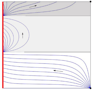
Streamlines for the induced flow solution (4.7) in a square box are plotted in figure 3 for (a) two-layer and (b) three-layer stratifications. The base layer is characterised by what may be regarded as a ‘smooth horizontal flush’: fluid entering through the lower opening moves nearly horizontally across the region (from right to left) thereby continuously flushing the layer. On approaching the left-hand wall, the induced flow tilts upwards before being entrained into the wall plume. Meanwhile, common to each layer above is an induced flow motion that is concentrated near the wall, adjacent to which is a region of near-stagnant fluid.

Figure 3. Induced flow patterns driven by a plane vertically distributed buoyancy source in a square emptying–filling box  $(\mathcal {A}=1)$ with the classic high- and low-level opening configuration. The equal-layer-depth stratification model of Linden et al. (Reference Linden, Lane-Serff and Smeed1990) and Cooper & Hunt (Reference Cooper and Hunt2010) is adopted. The step between two adjacent streamlines is $\Delta \psi =0.025$. Arrows indicate the general direction of flow. Dashed lines indicate interface positions. (a) Two-layer stratification, $n=1$. (b) Three-layer stratification, $n=2$.
Prior to exploring these flow patterns further, we proceed by questioning and subsequently relaxing the classic assumption of equal-depth layers (2.4). This allows for a refined prediction of the stratification whose induced flow we then evaluate and assess.
5. Ceiling flow regimes
Uncertainty regarding the precise details of the interaction between the wall plume and the ceiling necessitates the introduction of assumptions to model the outflow from the impingement region. The model for the classic stratification (Linden et al. Reference Linden, Lane-Serff and Smeed1990) implicitly assumes that, upon impingement with the ceiling (at  $y=1$), the entire body of buoyant fluid transported vertically in the wall plume is turned through a right angle to propagate as a horizontal current without further fluid exchange with the ambient. Although a useful model, the actual flow scenario near the ceiling may be quite different. Indeed, in the flow observations made by Cooper & Hunt (Reference Cooper and Hunt2010), layers of identical depth were not evident as the top layer was markedly thinner.
If one considers where the wall plume impinges with the ceiling, we note that the vertical momentum flux of the plume is reduced to zero and the volume flux transported by the plume provides the ‘source’ volume flux for the horizontal current. Hunt & Dyke (submitted), who consider the induced flow established by a localised line source at the base of an emptying–filling box, initially proposed to model the outflow from the impingement region into the ambient in two ways: first, in the spirit of a simplified model, as a potential flow source; however, this simplification means that the buoyant outflow need not remain attached to the ceiling as anticipated in practice; and second, as a turbulent ceiling jet, since entrainment can occur across the perimeter of the current if the shear is strong enough to overcome the stable stratification. Herein, we adopt the latter approach.
A final uncertainty we raise concerns the relative strengths of the ceiling current and the draining flow. If, for example, the upper opening area is too small to sustain the entire volume flux of the ceiling current, the excess fluid will impinge on the right-hand wall and potentially drive an overturning motion, as described by Kaye & Hunt (Reference Kaye and Hunt2007) for a current originating from the impingement of a point source plume. Remarkably little is currently known about overturning motions associated with steady flows in ventilated boxes and whilst ventilation flows driven by a range of different plume geometries have been investigated (Linden et al. Reference Linden, Lane-Serff and Smeed1990; Cooper & Linden Reference Cooper and Linden1996; Linden & Cooper Reference Linden and Cooper1996; Hunt & Linden Reference Hunt and Linden2001, Reference Hunt and Linden2005; Cooper & Hunt Reference Cooper and Hunt2010), to our knowledge these motions have not been reported in any detail. Moreover, acquiring meaningful experimental results on the ceiling flow scenarios is extremely difficult for a number of reasons. For example, when pumping saline solution through a porous wall to produce the plume in an aqueous environment (cf. Cooper & Hunt Reference Cooper and Hunt2010; Gladstone & Woods Reference Gladstone and Woods2014; Bonnebaigt et al. Reference Bonnebaigt, Caulfield and Linden2018) it is nearly impossible to maintain a uniform buoyancy flux. During the course of such an experiment the developing stratification reduces the flux of buoyancy from the wall and so the measurements made at a suitably large time are not those driven by the intended source conditions.
However, among the few, the experiments of Cooper & Hunt (Reference Cooper and Hunt2010) did suggest a representative ceiling flow regime. They observed that the ceiling current was well established without any indication of mixing associated with an energetic impingement at the ceiling, or evidence of overturning at the side wall opposite the plume source. Thus, in the flow regime they observed, the wall plume turned smoothly upon reaching the ceiling and the resulting current drained out totally through the upper opening without inducing an overturning motion.
In the modelling that follows (§ 6) we adopt this description of the flow, wherein we assume that net entrainment is present along the perimeter of the ceiling current. This assumption will be justified in § 7.6 on account of the high shear rate that we deduce from the induced flow solution.
6. Stratification with an entraining ceiling current
As proposed in § 5 and depicted in figure 1, for the top layer of the ceiling flow regime the sum of the volume fluxes entrained horizontally by the wall plume and vertically by the ceiling current over the interval  $[0,2a]$ must be equal to the ventilation flow rate $q_0$. Defining $q_{ce}(x)$ as the volume flow rate in the ceiling current, we therefore write
 \begin{equation} q_{ce}(x=2a)=q_0. \end{equation}
Continuity at the top-left corner requires
 \begin{align} q_{ce}(x=0)=q(y=1),\quad g'_{ce}(x=0)=g'(y=1),\quad d_{ce}(x=0)=b(y=1), \end{align}
where  $g'_{ce}(x)$ and $d_{ce}(x)$ denote the reduced gravity and the depth of the ceiling current. Thus, the depth-averaged horizontal velocity of the current $u_{ce}(x)=q_{ce}(x)/d_{ce}(x)$. To establish the dynamical condition of the ceiling current we define the ratio of the inertia and buoyancy forces at its source $(x=0)$ by means of the Froude number
 \begin{equation} Fr_s:=\frac{{u_{ce}(0)}}{\sqrt{g_{ce}^{'}(0)\,d_{ce}(0)}}. \end{equation}
With reference to (2.7a–d), (2.11) and (6.2a–c) we have
 \begin{equation} Fr_s=\left(\frac{4c_1}{3\alpha}\right)^{{3}/{2}}\approx 226. \end{equation}
Thus, given  $Fr_s \gg 1$ it is reasonable to neglect the role of the buoyancy force in the development of the ceiling current and proceed under the assumption that the dynamical aspects of the current are approximated by those of a horizontal wall jet.
The scalings and empirical relationships of Rajaratnam (Reference Rajaratnam1976) for a horizontal plane wall jet enable the local volume flux  $q_{ce}(x)$ and depth $d_{ce}(x)$ of the ceiling current to be expressed as
 \begin{equation} q_{ce}(x)=c_2q_{ce}(0)\sqrt{\frac{x-x_{vs}}{d_{ce}(0)}} \quad \text{and} \quad d_{ce}(x)=c_2^2(x-x_{vs}), \end{equation}
respectively. In (6.5a,b), the constant  $c_2=0.26$ (Rajaratnam Reference Rajaratnam1976) and $x_{vs}$ denotes the virtual source location of the ceiling current. By substituting $x=0$ into (6.5a,b), the location of the virtual source is
 \begin{equation} x_{vs}=-\frac{d_{ce}(0)}{c_2^2}= - \frac{3 \alpha h_1}{4 c_2^2}. \end{equation}
Substituting for (2.8) and (6.5a,b) into (6.1), and recalling that  $h_1=1-nh_0$, yields
 \begin{equation} (1-nh_0)^{{8}/{3}}+\left(4c_2^2a/(3 \alpha)\right) (1-nh_0)^{{5}/{3}} - h_0^{{8}/{3}}=0. \end{equation}
Re-deriving (2.10) without making the assumption of equal-depth layers gives
 \begin{equation} q_0=\frac{A}{\alpha H}\left(\int_0^1g'_e\,\mathrm{d} y\right)^{{1}/{2}}=\frac{A}{\alpha H}\left(\sum_{j=1}^{n} g'_{e,j}h_0+g'_{e,n+1}h_1\right)^{{1}/{2}}. \end{equation}
Substituting for (2.8) and (2.12) into (6.8) leads to the following cubic in  $h_0$:
 \begin{equation} 2c_1^3 \alpha^2\left(H/A\right)^2h_0^3+(n^2+n)h_0-2n=0. \end{equation}
To proceed, we note that on specifying  $n$ and $a=W/(2H)$, the two equations (6.7) and (6.9) form a closed system for the two unknowns $h_0$ and $A/H$.
At this stage it is useful to highlight some key distinctions between the classic model (1.1) and the approach taken herein. Distinct from other emptying–filling-box flows, whose steady states do not exhibit a dependence on the lateral dimension of the box (e.g. Linden et al. Reference Linden, Lane-Serff and Smeed1990; Linden & Cooper Reference Linden and Cooper1996; Gladstone & Woods Reference Gladstone and Woods2001; Hunt & Linden Reference Hunt and Linden2001, Reference Hunt and Linden2005), (6.7) clearly indicates such a dependence. Additionally, (1.1) only permits solutions for  $A/H$ that correspond to integer values of $n$. Our model overcomes this limitation given that a range of different $\{A/H,a\}$ corresponds to a given $n$ on account that the layer depths adjust due to entrainment by the ceiling current.
6.1. Predictions of layer depth and constraints on model
Before solving for the induced flow, it is informative to examine the refined stratification pattern and assess how it differs from the equal-depth-layer stratification. Figure 4 shows the correspondence between the number of layers  $n$ in a box with aspect ratio $\mathcal {A}=W/H$ and effective area $A/H$. A point of note is that $A/H$ cannot be prescribed a priori, but rather there is a unique value of $A/H$ that corresponds to a given number of interfaces for a box of aspect ratio $\mathcal {A}$. From a practical perspective, e.g. in a ventilated room, $A/H$ cannot be specified precisely, even if $a_l, a_u$ and $H$ can be. The underlying reason for this is that the discharge coefficient associated with the upper opening, $c_u$ in (1.2), has been shown by Hunt & Holford (Reference Hunt and Holford2000) and Holford & Hunt (Reference Holford and Hunt2001) to depend on the local Richardson number for flow through that opening – a quantity whose value is not known at the outset and would require a complex set of measurements in order to estimate. Moreover, on activating the wall plume, the value of $c_u$ will continuously adjust as the flow develops toward a steady state until ${(}\mathcal {A},A/H)$ falls onto a nearby contour of $n=\mathrm {constant}$ (figure 4); $c_l$ will also adjust as the Reynolds number of the flow through the lower opening increases (Ward-Smith Reference Ward-Smith1980). While for $n >2$ the stratification is insensitive to the box aspect ratio, decreasing the effective opening area $A/H$ tends to increase the number of layers. To achieve at least three layers requires $A/H<0.007$. Moreover, as the number of layers increases, the incremental reduction in $A/H$ that gives rise to an additional layer becomes increasingly small (figure 4).


Figure 5 illustrates how the layer depths,  $h_1$ (top layer) and $h_0$ (lower layers), vary with $n$ in a square box. The predictions of our model are shown ( $h_1$ solid line, $h_0$ dot-dashed line) together with those of Linden et al. (Reference Linden, Lane-Serff and Smeed1990) (dashed line). The depth of the lower layer we predict is greater than that predicted in Linden et al. (Reference Linden, Lane-Serff and Smeed1990) and the difference decreases with $n$. Evidently, the top layer is significantly thinner than the lower layers and thins on increasing $n$. The prediction of a markedly thinner top layer in this refined stratification model aligns well with the observations in Cooper & Hunt (Reference Cooper and Hunt2010). Our model predicts that $h_1 \rightarrow 0$ as $n \rightarrow \infty$. As such, for sufficiently large $n$, the top layer would only marginally exceed the depth of the ceiling current, turbulent entrainment into which could then erode the interface in practice. In such a case, our model breaks down and the potential coalescence of layers may offer a reason as to why the number of layers observed in experiments is limited to just a few. Insisting $d_{ce}(1)\ll h_1$, with reference to (6.5a,b), we obtain the following constraint:
 \begin{equation} h_1(\mathcal{A}=1)\gg\frac{c_2^2}{1-3\alpha/4} \approx 0.07. \end{equation}
Equivalently, an upper bound on the aspect ratio,  $\mathcal {A}=\mathcal {A}_{max}$, for which our model is valid may be acquired on letting $d_{ce}(\mathcal {A}_{max})=h_1$ in (6.5a,b), from which
 \begin{equation} \mathcal{A}_{max}=h_1 \left( \frac{1-3 \alpha/4 }{c_2^2} \right). \end{equation}
Substituting this and  $a=\mathcal {A}_{max}/2$ into (6.7), we obtain $\mathcal {A}_{max}(n=1)=3.25$ for a two-layer stratification and $\mathcal {A}_{max}(n=2)=1.83$ for a three-layer stratification.

Figure 5. The reduction in the dimensionless layer depth with the number of interfaces. The depths of lower layers  $h_0$ and top layer $h_1$ are plotted from the solution of (6.7) and (6.9). The Linden et al. (Reference Linden, Lane-Serff and Smeed1990) prediction, (1.1), is displayed for comparison. The red line, with scale given on the right-hand side vertical axis, plots the variation of $A/H$ with $n$: (a) $\mathcal {A}=1$; (b) $\mathcal {A}=1.46$, the aspect ratio used in the experiments of Cooper & Hunt (Reference Cooper and Hunt2010).
For a square box  $(\mathcal {A}=1)$, the constraint $h_1(\mathcal {A}=1) \gg 0.07$ (6.10) restricts the number of interfaces to no more than three (see $h_1$-curve in figure 5a). Cooper & Hunt (Reference Cooper and Hunt2010) used a box with dimensions $60\ \mathrm {cm}\times 41.2\ \mathrm {cm}\times 15\ \mathrm {cm}$ ( $W\times H\times L$) giving $\mathcal {A}=1.46$. For this geometry we require $h_1(\mathcal {A}=1.46) \gg 0.10$ which, with reference to figure 5(b), indicates that at most two interfaces should be possible – this is indeed what Cooper & Hunt (Reference Cooper and Hunt2010) observed.
7. Induced flow pattern
7.1. Solution for the refined stratification
The approach developed in §§ 2–4 remains valid for the new model of stratification (§ 6), but the boundary conditions for the top layer developed earlier need to be modified. Since the gradient of the streamfunction along the upper boundary is equal to the entrainment flux of the ceiling current, the boundary conditions for the top layer are
 \begin{equation}
\left.\begin{array}{cc@{}} \psi=-c_1 y^{{4}/{3}} &
\mathrm{on}\ x=-a\ \& \ 0\leqslant y\leqslant h_1 \\
\psi=-c_1c_2h_1^{{4}/{3}}\sqrt{\dfrac{2(x+a)}{3\alpha
h_1}+\dfrac{1}{c_2^2}} & \mathrm{on}\ -a\leqslant
x\leqslant a\ \& \ y=h_1 \\ \psi=-q_0 & \mathrm{on}\
\textrm{other boundaries}. \end{array}\right\}
\end{equation}
\begin{equation}
\left.\begin{array}{cc@{}} \psi=-c_1 y^{{4}/{3}} &
\mathrm{on}\ x=-a\ \& \ 0\leqslant y\leqslant h_1 \\
\psi=-c_1c_2h_1^{{4}/{3}}\sqrt{\dfrac{2(x+a)}{3\alpha
h_1}+\dfrac{1}{c_2^2}} & \mathrm{on}\ -a\leqslant
x\leqslant a\ \& \ y=h_1 \\ \psi=-q_0 & \mathrm{on}\
\textrm{other boundaries}. \end{array}\right\}
\end{equation}
On applying the conformal mapping (4.1), the physical boundaries map to the real axis of the  $w$-plane with the following boundary conditions
 \begin{equation} \varPsi=\left\{\begin{array}{@{}ll@{}}
-c_1c_2h_1^{{4}/{3}}\sqrt{\dfrac{2(C\,\mathrm{sn}^{-1}(u)+a-\textrm{i}h_1)}{3\alpha
h_1}+\dfrac{1}{c_2^2}} & u<-\dfrac{1}{k} \\
-c_1[-\textrm{i}(C\,\mathrm{sn}^{-1}(u)+a)]^{{4}/{3}} &
-\dfrac{1}{k}\leqslant u< -1 \\ -q_0 & -1\leqslant u<1/k \\
-c_1c_2h_1^{{4}/{3}}\sqrt{\dfrac{2(C\,\mathrm{sn}^{-1}(u)+a-\textrm{i}h_1)}{3\alpha
h_1}+\dfrac{1}{c_2^2}} & u\geqslant 1/k.
\end{array}\right\}
\end{equation}
\begin{equation} \varPsi=\left\{\begin{array}{@{}ll@{}}
-c_1c_2h_1^{{4}/{3}}\sqrt{\dfrac{2(C\,\mathrm{sn}^{-1}(u)+a-\textrm{i}h_1)}{3\alpha
h_1}+\dfrac{1}{c_2^2}} & u<-\dfrac{1}{k} \\
-c_1[-\textrm{i}(C\,\mathrm{sn}^{-1}(u)+a)]^{{4}/{3}} &
-\dfrac{1}{k}\leqslant u< -1 \\ -q_0 & -1\leqslant u<1/k \\
-c_1c_2h_1^{{4}/{3}}\sqrt{\dfrac{2(C\,\mathrm{sn}^{-1}(u)+a-\textrm{i}h_1)}{3\alpha
h_1}+\dfrac{1}{c_2^2}} & u\geqslant 1/k.
\end{array}\right\}
\end{equation} Substitution of (7.2) into (4.7) yields the solution for the induced flow in the top layer. Although now of an increased height, the solution for the flow in any of the lower layers is unchanged from that developed in § 4. The induced flow solution for the stratification in a square box with ceiling current is plotted in figures 6(a)–6(c) for  $n=1$, $2$ and $3$, respectively.

Figure 6. Induced flow patterns in a square emptying–filling box ( $\mathcal {A}=1$) driven by a plane vertically distributed buoyancy source with ceiling current; (a) $n=1$, (b) $n=2$, (c) $n=3$. The step between adjacent streamlines is $\Delta \psi =0.025$. Arrows indicate the general direction of flow. The position of each interface is shown as a horizontal line; the solid part of the line represents where the interface is predicted to be linearly stable (and the dotted part, unstable) based on the simplified analysis of § 7.6.
7.2. General flow pattern
A first point of note is that the general pattern of flow in each type of layer, types which we shall refer to as the top, intermediate and base layers, remains unchanged regardless of the number of interfaces  $n$ (figure 6). To assist the following discussion, the distribution of dimensionless flow velocity magnitude $U(x,y)$ for the three-layer case, corresponding to the streamline plot figure 6(b), is plotted in figure 7.

Figure 7. Colour map and contours showing the distribution of dimensionless velocity magnitude  $U(x,y)$ corresponding to the streamline pattern for $\mathcal {A}=1$ and $n=2$ shown in figure 6(b). (a) Top layer. (b) Intermediate layer. (c) Base layer. The velocity associated with each colour is indicated on the horizontal scale above (a).
Entering through the lower opening at ( $x=1,y=0$), the flow turns smoothly and is drawn near horizontally towards the buoyancy source (left wall, $y$-axis). Interestingly, the streamlines tend to tilt upwards at the left wall in response to the wall-plume entrainment. Evidently, the flow in the upper-right region of the base layer is relatively slow (figure 7c).
The flow in the bulk of the intermediate layer (figure 6b), or intermediate layers (figure 6c), is near stationary. The majority of the motion is confined to the region adjacent to the left wall. This motion is created as buoyant fluid, discharged into an intermediate layer from the outflow of the wall plume below, is re-entrained into the wall plume of the intermediate layer. The existence of the large-scale quiescent region (figure 7b) implies that, for the application of room ventilation, the air is stale at middle heights. As highlighted in appendix A, correctly locating the lower opening is crucial to avoid similar large-scale regions of stale air within the base layer. Designers should ensure that the stale region is above the height,  $H_l\,$ (m), of the living zone. The corresponding design criterion is $h_0(n,\mathcal {A})>H_l/H$.
The streamline pattern in the top layer is most easily appreciated in figure 6(a). Immediately above the interface and adjacent to the wall plume, the flow pattern is similar to that in any intermediate layer. While a portion of the volume flux supplied to the top layer from below is transported by entrainment towards the left wall, the bulk forms the ceiling current. The region near the upper opening (at  $x=1$, $y=1$) is relatively quiescent, cf. figure 7(a).
7.3. Velocity magnitude distribution
With reference to figure 7, the velocity magnitude  $U$ within each layer is the highest at the region of inflow, and gradually decays away from this region. In the base layer, the velocity magnitude in the central region is between $U=0.5$ and $U=0.6$, and relatively uniform; elsewhere, $U$ tends to increase towards the upper-left and lower-right corners, and decreases towards the other two corners. In the intermediate layer, at locations sufficiently far away from the inflow (here for $x \gtrsim 0.3$), $U$ varies little with height but primarily with the horizontal coordinate, as illustrated by the near-vertical iso-lines. Moving away from the left wall, $U$ declines so quickly that more than three-fifths of the layer has a velocity magnitude of less than $0.1$. Since, according to the scalings (2.5a–d), $U=0.1$ is equal to the plume velocity at the height $y=1/800$, the induced flow is generally weak compared with the primary plume motion. Though lacking immediate practical interest due to its location, the induced flow pattern in the top layer is distinct and worthy of comment. The bulk flow is the most rapid of the three layers and has a complex distribution of velocity. In the central and right sides of this layer, the velocity magnitude is mainly dependent on the horizontal coordinate (cf. the intermediate layer). Interestingly, along the ceiling, the velocity magnitude has a maximum at $x=0.15$ (to 2 s.f.), which results directly from the specific profile adopted that accounts for entrainment into the ceiling current, (6.5a,b).
To gain further insight into how the velocity magnitude varies spatially, figure 8 displays the variation of  $U(x=\text {const.},y)$ along three vertical sections in the box, $x=\{0.25,0.5,0.75\}$. For convenience, the depth of each layer is scaled so as to have unit height. The velocity magnitude in the base layer shows more vertical variation, but less horizontal variation than the intermediate and top layers; there is a velocity increase with height on the left side of the box ( $x=0.25$) and a decrease on the right side ( $x=0.75$). For the intermediate layer, all three profiles exhibit low velocity magnitudes (consistent with the large-scale, near-stagnant region reported in § 7.2) and little variation with height. The velocity magnitude in the top layer is generally high (exceeding $U=0.9$ on $x=0.25$) while the vertical variation is relatively slight.

Figure 8. Vertical profiles of dimensionless velocity magnitude  $U$ at a quarter ( $x=0.25$), a half ( $x=0.5$) and three quarters ( $x=0.75$) of the box width from the wall plume; $\mathcal {A}=1$, $n=2$. (a) Top, (b) intermediate and (c) base layer. Here, $\Delta y$ denotes the vertical distance from the base of each layer.
7.4. Controlling the induced flow
In practical terms, the area of the openings and the room aspect ratio,  $\{A/H,\mathcal {A}\}$, are the two key quantities that are available to a ventilation engineer at the design stage to control the induced flow. Since the number of interfaces can be estimated from figure 4, by experience, or by estimating $A/H$, the two controllable variables are chosen to be $n$ and $\mathcal {A}$ in the following discussion (as is consistent with § 6).
We note from figure 6 that the number of interfaces has little effect on the fundamental pattern of flow in any type of layer but significantly influences the dimensionless velocity magnitude  $U$ within the whole box. With more layers, $U$ declines rapidly, which results from the decreasing ventilation flow rate $q_0$. Take the base layer for instance. The spatially averaged velocity magnitude, $\bar {U}$, defined as the ventilation flow rate divided by layer depth, is
 \begin{equation} \bar{U}:= q_0/h_0\sim h_0^{{1}/{3}}. \end{equation}
The reduction of  $h_0$ with $n$ leads to overall slower motion with correspondingly sparser streamlines. Similar arguments may be applied to the top and intermediate layers.
When  $n$ increases from one to three, the velocity magnitude $U$ in the base layer declines almost by half. In the meantime, the stale air region in the intermediate layer widens considerably. Thus, to enhance the natural ventilation, $n$ should be as small as possible, which is primarily achieved with larger effective opening areas $A/H$.
Figure 9 highlights the role of box aspect ratio  $\mathcal {A}$ in the induced flow for (a) $\mathcal {A}=0.5$ and (b) $\mathcal {A}=1.5$. Evidently, the general flow pattern is weakly dependent on $\mathcal {A}$, which is relatively unchanged despite the factor of three increase in $\mathcal {A}$. There is, however, a marked decrease in the depth of the top layer and increase in the velocity magnitude within the layer. The latter increase is due to the reduced top layer depth transporting the increased volume flux that has resulted from the deepening of the lower layers. By comparison, the velocity magnitude in the lower layers only changes slightly. Interestingly, with increasing $\mathcal {A}$, the streamlines in the base layer indicate an increasingly uniform flow, a desirable characteristic for the ventilation of many rooms. Despite this, there is a widening of the near-stagnant region in the intermediate layer, which is undesirable.

Figure 9. Colour map of dimensionless velocity magnitude  $U(x,y)$ overlain with streamline pattern for the $n=2$ stratification; (a) $\mathcal {A}=0.5$, (b) $\mathcal {A}=1.5$. The step between two adjacent streamlines is $\Delta \psi =0.05$. The vertical colour bar indicates the magnitude of the dimensionless velocity.
7.5. A comment on box size and wall buoyancy flux
The box size, as fully specified by the box height  $H$
$H$  $(\mathrm {m})$ for a given aspect ratio $\mathcal {A}$, and the source buoyancy flux $\chi$ $(\mathrm {m}^2\ \mathrm {s}^{-3})$ have no effect on the dimensionless induced flow field since they both vanish in the non-dimensionalisation. Nevertheless, on dimensional grounds (2.5a–d), the velocity magnitude $U \propto H^{{1}/{3}}\chi ^{{1}/{3}}$ and the buoyancy $g'_e \propto H^{-{1}/{3}} \chi ^{{2}/{3}}$. For given $(n,\mathcal {A})$, there is no change to the pattern of flow on increasing $\chi$ or $H$. However, there will be an increase in the magnitude of the velocity. Moreover, the layer buoyancy and the buoyancy jump across each interface increase with $\chi$ and decrease with $H$.
$H$.
7.6. Stability of interfaces and instability of ceiling jet
All solutions above for the induced flow suggest a velocity jump and, thereby, a shear flow at each interface and between the perimeter of the ceiling current and its surroundings. The destabilising influence of the shear competes against the stabilising stratification, potentially leading to a breakdown of the flow through the Kelvin–Helmholtz mechanism. Previously, Cooper & Hunt (Reference Cooper and Hunt2010) suggested that interfacial instability might be the reason that fewer interfaces were observed than predicted. For this reason, it is prudent to assess the stability of the situation we predict via a simplified analysis. The corresponding linear stability criterion, developed by Taylor–Goldstein (Turner Reference Turner1979, Chapter 4), is well established as
 \begin{equation} \frac{{\rm \pi}\Delta u^2}{\lambda\Delta g_e'}<1, \end{equation}
where  $\Delta u$ and $\Delta g_e'$ denote the jump in the horizontal component of flow velocity and layer buoyancy, and $\lambda$ is the wavelength of a normal mode perturbation. For stability, the above criterion needs to be satisfied for the longest possible wavelength $\lambda =2a$, i.e. a wavelength equal to the width of the box.
For each interface  $\Delta g_e'=c_1^{-1}h_0^{-1/3}$ from (2.12), and hence (7.4) may be written in terms of an interfacial critical velocity jump, $\Delta u_{crit}$
 \begin{equation} \Delta u<\sqrt{\frac{2a}{{\rm \pi} c_1 h_0^{{1}/{3}}}}=\Delta u_{crit}. \end{equation}
As the velocity jump  $\Delta u$ varies with $x$ (figure 7), the stability situation may vary along each interface. For the ceiling current, stability would require $\Delta u< \Delta u_{crit,ce}$, and we take $\Delta u$ to be that at the source $(x=0,y=1)$ as here the velocity jump between current, with an average velocity of $q_{ce}(0)/d_{ce}(0)$, and ambient is the greatest.
The corresponding stability parameters for  $n=1$, $2$ and $3$ in a square box are given in table 1. Column three shows that an interface is stable on the right-hand side but linearly unstable on the left-hand side. With the stable locations being marked with solid lines in figure 6, the length of the unstable part increases markedly with decreasing $n$. While it is likely that viscosity and nonlinear effects stabilise the unstable part of an interface in practice, it should also be noted that criterion (7.4) fails at the left end of an interface because two of the assumptions underlying (7.4), i.e. potential flow and uniform streams, break down there. Comparing columns four and five, $\Delta u \gg \Delta u_{crit,ce}$ is consistent with a turbulent ceiling current.
Table 1. Entries (to 2 s.f.) relating to the stability, or otherwise, of the interfaces between layers and the ceiling current.  $\mathcal {A}=1$.

8. Discussion and conclusion
We considered the steady flow that a turbulent wall plume induces in an emptying–filling box where openings, slots made in the base and top of the box, connect the interior to a uniform, quiescent exterior. Previous developments focus, almost exclusively, on the stratification, modelling this as a stack of equal-depth layers. Our focus has instead been on the development of a simplified theoretical model for predicting the streamline pattern and velocity distribution within the layers. These important aspects of the flow had not been examined previously, either theoretically or experimentally, despite having important practical implications for achieving comfort in naturally ventilated buildings and for the indoor spread of airborne contagions, such as an influenza virus. These flows can be induced in a room by a wall or glass façade heated by the Sun (or for the vertical inversion of the case we consider, cooled by the exterior air) and our primary motivation has been to gain insights into the patterns of flow established in ventilated buildings, together with a grasp of the parameters that control them.
Our contribution is essentially fourfold. First, for the ‘classic’ stratification of equal-depth layers, we developed closed-form solutions for the streamfunction that describe the wall-plume-induced flow within each layer. Second, recognising that the classic stratification neglects the flow near the ceiling, we introduced an entraining ceiling current hypothesis and the corresponding theoretical description of the resulting stratification, removing the need to assume that all layers have equal depth. This re-evaluation of the stratification highlighted the dependence of the layer depths on the entraining current. Third, we solved for the induced flow for the refined stratification and, finally, assessed the implications of our predictions for stratified flows in ventilated rooms. Cooper & Hunt (Reference Cooper and Hunt2010) comment that persistent interfaces are hard to maintain in experiment and, whilst this could be attributed to the challenges of achieving and maintaining a source of uniform and constant buoyancy flux, this provided motivation for us to consider the stability of the interfaces. In principle, the simplified linearised analysis we present serves only to justify that the interfaces can be stable in general cases and, via this analysis, we can be more confident about the stratification model we present. A full investigation of the interfacial stability, including nonlinear effects and viscosity, would likely offer considerable additional insight although this falls outside the immediate scope of our work.
Working in the complex plane, conformal mapping techniques and Poisson's integral theorem were deployed to solve for the flow induced within each layer, with the boundary conditions established by treating the wall plume as a vertical line of sinks. Advantages of this approach over alternatives include the ability to rapidly re-evaluate the solution on altering the dimensions and locations of the openings (appendix A), and the ease with which multiple additional openings can be included.
In existing emptying–filling-box studies, where turbulent entrainment occurs solely over the vertical rise of the plume, layer depths depend exclusively on the dimensionless effective opening area. The inclusion of an entraining horizontal current reveals an additional dependence, namely, on the box aspect ratio  $\mathcal {A}=W/H$, taken herein as width relative to height, and a top layer that is thinner than the other layers and which adjusts in depth with effective opening area. According to our model, the layers can only have equal depth if there is no entrainment by the ceiling current. Increasing $\mathcal {A}$ causes a reduction in the depth of the top layer and an increase in the depth of the layers below, while the number of interfaces $n$ shows a weak tendency to increase with $\mathcal {A}$. Overlooking the ceiling current, which contributes significantly to overall entrainment, the classic model of stratification leads to an underestimation of the ventilation flow rate.
The flow patterns characterising the base layer, intermediate layer(s) and top layer that comprise the stratification each have distinguishing characteristics which vary only quantitatively with  $n$ and $\mathcal {A}$. The source buoyancy flux $\chi$ $(\mathrm {m}^2\ \mathrm {s}^{-3})$ and box size (referring to box height $H$
$H$  $(\mathrm {m})$ for a given aspect ratio) have no influence on the patterns of flow but determine the velocity magnitude, which scales as $\chi ^{{1}/{3}}$ and $H^{{1}/{3}}$. Consistent with the classic stratification, the dimensionless velocity magnitude declines significantly in each layer with $n$. Moreover, the buoyancy of the top and intermediate layers increases with $\chi$ but decreases with $H$.
$H$.
Although our wall-jet hypothesis excludes the effect of the stratification on the ceiling current, and thus may overestimate entrainment, this has little impact on the prediction of the induced flow pattern within the lower layers which is of paramount interest for the application to room ventilation. While there is evidence that a lateral ceiling current produces mixing along its perimeter (e.g. Kaye & Hunt Reference Kaye and Hunt2007), there are currently no detailed measurements that we are aware of that are specific to the wall-plume emptying–filling box considered herein. Beyond the unresolved complication of achieving a uniform source buoyancy flux and that specifying the effective opening area a priori is simply not possible, analogue experiments (cf. Cooper & Hunt Reference Cooper and Hunt2010) are notoriously difficult to conduct and so a more detailed quantitative validation of our predictions is not currently possible. Even so, we have smoothly varying predictions of stratification across a spectrum of effective opening areas and gained a first insight into the streamline pattern and velocity distribution. That stated, our approach is simplified, and although, according to Cooper & Hunt (Reference Cooper and Hunt2010), experimental difficulties lead to a departure from the target, idealised wall-plume boundary conditions, some of the previous experiments exhibited vertical density gradients within layers and evidence of detrainment from the wall plume (Gladstone & Woods Reference Gladstone and Woods2014). As such, we suggest that the current model be applied in cases when entrainment is dominant along the wall plume, i.e. for a wall plume with relatively high local Richardson numbers.
Finally, from the perspective of airflow in buildings, both in terms of achieving comfort for natural ventilation and with regards to the movement of passive airborne contaminants or fine aerosol mists by the induced flow, our results indicate that (i) the choice of location of the lower opening is crucial to successfully ventilating the lower layer given it can lead to a desirable smooth flushing of this region or to a large-scale region of near-stagnant air and (ii) intermediate layers are characterised by large-scale stagnant regions, irrespective of opening location. We end with a cautionary note regarding the direct application of our work to room ventilation where the movement of occupants, an external wind flow or variations in the solar heat gains received by a façade would cause a departure from the idealised, albeit already complex, steady situation we have considered. Whilst this idealisation has offered new insights into the airflow patterns induced and a simplified predictive capability, the situation in practice is unquestionably far more complex and such well-defined layers may not form.
Acknowledgements
The authors are grateful to three anonymous referees for their helpful comments on an earlier draft.
Funding
G.R.H. would like to express his gratitude to Dyson Technology Ltd for their ongoing support and to the EPSRC through grant no. EP/N010221/1, entitled Managing Air for Green Inner Cities (MAGIC).
Declaration of interests
The authors report no conflict of interest.
Appendix A. Wider applicability: general configurations and finite-width openings
By contrast with alternative methods of solution, e.g. separation of variables, the conformal mapping approach developed above can be applied with ease to obtain closed-form solutions for the streamline pattern in emptying–filling boxes with openings of arbitrary width and location. The general form of the induced flow solution (4.7), as expressed in terms of  $\varPsi (\xi ,0)$, for each layer in the mapped domain is unchanged. It is convenient here to express this solution as
 \begin{equation} \varPsi(u,v)=\frac{v}{\rm \pi}(I_1+I_2+I_3+I_4+I_5), \end{equation}
where  $I_k\,(k=1,\ldots , 5)$ refers, in order, to the five integrals in (4.7). In the classic configuration, $\varPsi (\xi ,0)$ is determined from the boundary conditions (4.4) for the base layer, (4.5) for an intermediate layer and (7.2) for the top layer.
For a lower opening centred on  $x=x_l$ with finite width $a_l$, with the stratification unaffected, only the boundary condition along the base of the box needs to be modified. With the classic high Reynolds number assumption of a uniform inflow velocity profile, the original boundary condition at the lower opening is replaced with a linearly varying streamfunction. Thus, only the solution for the base layer is altered and this change is
 \begin{equation} I_3=\int_{\xi_1}^{\xi_2} -\frac{q_0}{a_l}\left(C\,\mathrm{sn}^{-1}\xi-x_l+\frac{a_l+1}{2}\right)\mathrm{d}\xi +\int_{\xi_2}^1-q_0\,\mathrm{d}\xi, \end{equation}
where  $\xi _1=\mathrm {sn}((x_l-a_l/2)/C)$ and $\xi _2=\mathrm {sn}((x_l+a_l/2)/C)$. To acquire the solutions plotted in figure 10(a–c), one needs to substitute into (A2): (a) $x_l=0.5$ and $a_l=0$; (b) $x_l=0.925$ and $a_l=0.15$; and (c) $x_l=0.5$ and $a_l=0.15$, respectively.

Figure 10. Streamlines superimposed on a colour map of velocity magnitude for four opening configurations in a square box with  $n=2$. The buoyancy source is uniformly distributed along the left wall ( $y$-axis). The deviations from the opening configurations examined in §§ 6 and 7 are (a) lower opening moved to mid-point of base, (b) lower opening of finite width $0.15$, (c) lower opening of finite width $0.15$ centred at mid-point of base and (d) top opening moved to mid-point of ceiling. The black dots indicate opening location and width. The increment between adjacent streamlines is $\Delta \psi =0.05$.
For an upper opening centred at  $x=x_u$, the formulation of a practical boundary condition at the ceiling, accounting for the interaction of the current with buoyancy-driven flow toward the opening, would appear to be extremely complicated and beyond the scope of this study. Indeed, not only could the current horizontally overshoot the location of the upper opening but the variation of volume flux across the opening, affected by the outflow, is expected to deviate considerably from that of the ceiling jet. However, to demonstrate the applicability of our solution approach, we adopt the boundary condition for an ‘ideal’ ceiling current which drains out totally through a point opening without horizontal overshooting. The stratification needs to be re-determined by replacing (6.1) with $q_{ce}(x_u)=q_0$, thereby accounting for the reduction in entrainment along the ceiling current. Based on the updated stratification, the boundary condition at locations to the right of the upper opening becomes $\psi =-q_0$. Only the induced flow solution for the top layer is altered. Defining $\xi _3=\mathrm {sn}((x_u-1/2+\textrm {i}h_1)/C)$, the change, with reference to (A1), is
 \begin{equation} I_1=\int_{-\infty}^{\xi_3}-q_0\,\mathrm{d}\xi+\int_{\xi_3}^{-1}-c_2q_0 \sqrt{\frac{2(C\,\mathrm{sn}^{-1}(u)+a+1/2-\textrm{i}h_1)}{3\alpha h_1}+\frac{1}{c_2^2}}\,\mathrm{d}\xi, \end{equation}
when  $x_u\leqslant 0.5$, or
 \begin{equation} I_5=\int_{1}^{\xi_3}-q_0\,\mathrm{d}\xi+\int_{\xi_3}^{\infty}-c_2q_0\sqrt{\frac{2(C\, \mathrm{sn}^{-1}(u)+a+1/2-\textrm{i}h_1)}{3\alpha h_1}+\frac{1}{c_2^2}}\,\mathrm{d}\xi, \end{equation}
when  $x_u>0.5$. Substituting $x_u=0.5$ into (A3) leads to the solution shown in figure 10(d).
A few features of the induced flows generated with these opening configurations in figure 10 are worthy of mention. First is the appearance of a region of near-stagnant fluid forming to the right side of the opening in the base layer on moving the lower opening (figure 10a,c). Second, if not too wide ( $a_l\ll 1$), the width of a lower opening does not significantly alter the induced flow pattern (compare figure 10a with 10c), other than adjacent to the opening.


 Open access