


1. Introduction
Turbulent, buoyant plumes are flows that arise from isolated sources of buoyancy, which include sources of heat, as well as injections of buoyant fluid. The interaction of multiple turbulent plumes in close proximity occurs in a wide range of environmental and industrial applications, such as smoke from chimneys, ventilation flow in restricted spaces, hydrothermal vents and multiple air pollution sources. Plume interaction, either with other plumes or with domain boundaries, can give rise to significantly modified flow behaviour in the near-source region (Cenedese & Linden Reference Cenedese and Linden2014; Li & Flynn Reference Li and Flynn2021).
Extensive research has been carried out on the bulk movement of fluid by plume entrainment in the built environment. Natural ventilation models can be used to approximate plumes rising from multiple heat sources and act as guidance when designing a room with sufficient air movement for occupants to be comfortable (Linden, Lane-Serff & Smeed Reference Linden, Lane-Serff and Smeed1990; Durrani et al. Reference Durrani, Cook, McGuirk and Kaye2011). Additionally, the interaction of multiple plumes has been investigated in an unrestricted domain with applications to climate and atmospheric modelling (Mokhtarzadeh-Dehghan, König & Robins Reference Mokhtarzadeh-Dehghan, König and Robins2006; Rooney Reference Rooney2015).
Thus far, most studies have examined plume interaction from a common baseline, i.e. with multiple sources at the same height. The work to be presented here extends the plume-interaction model of Rooney (Reference Rooney2015, Reference Rooney2016) to the case of two sources with a vertical as well as a horizontal offset. This opens the way for quantification of the effects of vertical offsets on flow in the near field. This can certainly occur in building ventilation problems with heat sources at different levels, and also in atmospheric convection at different heights. Furthermore, plume interaction from sources with a vertical offset occurs between thermal vents in the ocean positioned at different heights above the ocean floor.
This study focuses on the morphology of the entrainment field in the plume environment. The entrainment flow is weak compared with the mean vertical velocities within the plume, but previous work (Rooney Reference Rooney2016) indicated the significance of entrainment for defining the plume boundary. This in turn affects the evolution of the other plume characteristics. For the cases studied here, the ambient flow structures provide a way to compare theory with numerical experiments.
The relative weakness of entrainment flows makes them potentially difficult to measure, either in experiments or in time-varying numerical simulations. They are, however, more accessible using computational fluid dynamics (CFD) simulations. In particular, time-averaged flows using the Reynolds-averaged Navier–Stokes (RANS) formulation provides a good representation of many aspects of single plume flow (Hargreaves, Scase & Evans Reference Hargreaves, Scase and Evans2012; Kumar et al. Reference Kumar, Mukherjee, Chalamalla, Dewan and Balasubramanian2022). Also, studies of multiple plumes using RANS (Durrani et al. Reference Durrani, Cook, McGuirk and Kaye2011; Lou et al. Reference Lou, He, Jiang and Han2019) have shown good comparison with the theoretical and experimental results of Kaye & Linden (Reference Kaye and Linden2004). However, the near-field entrainment of vertically offset sources has not been investigated. Therefore, RANS will be used to examine both the interacting plumes and their environment. Some possible indications of limits on the capability of RANS in this context will also be discussed.
We begin by presenting some background literature on the dynamics of a single plume in § 2, which is necessary to develop the new analytical theory in § 3. Details of the numerical simulation are presented in § 4. In § 5 we validate and verify our single plume and the no vertical offset case against existing theory and experiments, before comparing our theoretical model and RANS results for the case of vertically offset plumes.
2. Dynamics of a single plume
2.1. Similarity model of a pure plume
The fluid in a plume moves under gravity and is driven by a density difference between the plume fluid and its surrounding environment. The plume body exhibits significant mean vertical velocity  $w$ and reduced gravity $g'$. The reduced gravity $g'$ is defined as $g' = {g(\rho _a-\rho )}/{\rho _0}$, where $\rho _a$ and $\rho$ denote the density of the ambient fluid and the plume, respectively, $\rho _0$ is some reference density and $g$ is the acceleration due to gravity. The radial profiles of these time-averaged quantities are approximately Gaussian, and may be represented as
 \begin{gather} \tilde{w} = C_w{F_0}^{1/3} z^{{-}1/3}\exp{({-}r^2/\tilde{b}^2)}, \end{gather}
 \begin{gather}\widetilde{g'} = C_{g'}{F_0}^{2/3} z^{{-}5/3}\exp{({-}r^2/\tilde{b}^2)}, \end{gather}
where  $\tilde {w}(r,z)$ is the vertical velocity, $\widetilde {g'}(r,z)$ is the reduced gravity, $\tilde {b}(z)$ is the $e$-folding length, $r$ is the radial or cross-plume coordinate, $z$ is the vertical coordinate, and $C_w$ and $C_{g'}$ are constants. In the self-similar regime, $\tilde {b} \propto z$. A small difference in the $e$-folding length scale between the two profiles is often observed, but also often assumed negligible so that the approximation of a single length scale is made, as above.
Such buoyant plumes are typically modelled with integral models. The classical model of Morton, Taylor & Turner (Reference Morton, Taylor and Turner1956) comprises a set of three coupled ordinary differential equations, which are based on three main assumptions: self-similarity, Boussinesq approximation and the constant entrainment coefficient  $\alpha$. In an unstratified environment the equations for volume flux $Q$, momentum flux $M$ and buoyancy flux $F$ are
 \begin{equation} \frac{\text{d}Q}{\text{d}z}=2 \alpha M^{1/2} , \quad \frac{\text{d}M}{\text{d}z} = 2 \frac{QF}{M} , \quad \frac{\text{d}F}{\text{d}z} = 0. \end{equation}
The ‘top-hat’ formulation replaces the peak values of  $w$ and $g'$ and the Gaussian $e$-folding length scale with horizontally averaged values of $w$ and $g'$ and an associated mean radius $b$. The fluxes can then be expressed as
 \begin{equation} Q = b^{2}w, \quad M=b^{2}w^{2}, \quad F = b^{2}wg'. \end{equation}
From here on, we use  $w(z)$ and $g'(z)$ to denote the top-hat variables, replacing the Gaussian profiles of $\tilde {w}(r,z)$ and $\widetilde {g'}(r,z)$, respectively.
In the formulation of these equations it is assumed that the plume originates from a point source. In actuality, plumes will begin from a source with some finite radius. To account for the finite nature of the source, one can extrapolate the sides of the plume back to some point origin, as shown in figure 1(a). This virtual origin correction is made by taking the height as  $z+z_v$ (when calculating the plume radius by the similarity solution (2.5), for instance), where $z_v$ is the height of the finite source above the virtual point source. At larger heights when $z \gg z_v$, the virtual origin correction will be negligible.

Figure 1. The configuration of two plumes with vertical offset  $\zeta$ and horizontal source separation $\chi$ shown in the $(a)$
$(a)$  $xz$ plane and $(b)$
$(b)$  $xy$ plane. The ‘lower’ plume is on the left and the ‘upper’ plume is on the right. The origin of coordinates $O$ is positioned along the centreline of the lower plume at the height of the upper plume virtual origin such that the virtual origin of the lower plume is at $(0,0,-\zeta )$, and that of the upper is at $(\chi,0, 0)$. The shaded circular region shows the cross-sectional area of the lower plume at $z=0$.
Under the assumption that the ambient fluid is of uniform density ( $\rho _0 \equiv \rho _a$), Morton et al. (Reference Morton, Taylor and Turner1956) give a similarity solution for an axisymmetric pure plume as
 \begin{gather} b = \frac{6\alpha}{5}z, \end{gather}
 \begin{gather}w = \frac{5}{6\alpha}\left(\frac{9}{10}\alpha F\right)^{1/3}z^{{-}1/3} , \end{gather}
 \begin{gather}g' = \frac{5F}{6\alpha}\left(\frac{9}{10}\alpha F\right)^{{-}1/3} z^{{-}5/3}. \end{gather}
2.2. The sink model of entrainment
A line sink of strength  $-m(z)$ positioned at the origin has complex potential
 \begin{equation} \varOmega ={-}\frac{m}{2{\rm \pi}}\ln Z, \end{equation}
where  $Z = x+{\rm i}y = r\text {e}^{\text {i}\theta }$. Since the flow induced by plume entrainment is horizontal and irrotational, Kaye & Linden (Reference Kaye and Linden2004) used line sinks to represent the flow exterior of two interacting plumes.
The principle of superposition implies that the complex potentials of individual line sinks can be summed to give a total complex potential representing the entrainment field of an equivalent configuration of interacting plumes. The real part of the resulting complex potential  $\varOmega = \phi + \text {i}\psi$ corresponds to the velocity potential.
As described previously by Rooney (Reference Rooney2015) and Rooney (Reference Rooney2016), contours of equal velocity potential can be used to approximate the mean plume boundaries at any height. Outside the plume boundaries, the streamfunction from the complex potential yields the combined horizontal entrainment field of multiple plumes. The vertical evolution of the system is controlled by the buoyancy of the plumes and the entrainment along the perimeter of the plume system. The distortion and merging of the plume boundaries is mirrored by that of the velocity-potential contours (e.g. Rooney Reference Rooney2016, figure 7).
3. Sink model for vertically offset sources
A diagram of two equal strength plumes emerging from point sources with horizontal separation  $\chi$ and vertical offset $\zeta$ is shown in figure 1. We will assume that the lower plume is unaffected by the upper plume until it reaches the height of its source. Under this assumption, the plume will rise as an axisymmetric plume and will have some radius $R$ when it reaches the upper plume source at height $z=0$. As such, its entrainment field cannot be approximated by a line sink. Instead, the flow on a horizontal cross-section taken at this height could be approximated by a circular sink of radius $R$ at the origin next to the line sink of the upper plume at a distance $\chi$ along the $x$ axis, as emphasised in figure 1(b). To represent this plume configuration, the existing circle theorem of Milne-Thomson (Reference Milne-Thomson1940) may be adapted such that a circle inserted into the flow is identified as a velocity-potential contour, rather than a streamline. In this way, the circle can be identified as the lower plume boundary at $z=0$. To produce net entrainment into the lower plume, a second line sink concentric with the circular boundary must also be incorporated.
3.1. A modified circle theorem
The circle theorem of Milne-Thomson (Reference Milne-Thomson1940) expresses how an irrotational, two-dimensional flow of incompressible and invisid fluid is altered upon the insertion of a circular cylinder into the flow. The circle of radius  $R$ obtained from a cross-section of the cylinder is denoted $C$ and has the equation $\lvert Z \rvert = R$. The theorem applies when the complex potential of the initial flow $f(Z)$ has no rigid boundaries and no singularities in the region $\lvert Z \rvert \leqslant R$ for $R \in \mathbb {R}$. Placing the circle into this flow changes the complex potential to
 \begin{equation} \varOmega(Z) = f(Z) + \overline{f\left({R^2}/{\bar{Z}}\right)}, \end{equation}
where the bar denotes the complex conjugate. Since  $R^2/\bar {Z}$ is the reflection of $Z$ in $C$ and $\lvert Z \rvert > R$ implies $\lvert R^2/\bar {Z}\rvert < R$, it follows that the additional, perturbing term has no singularities outside of $C$. Furthermore, the circle is a streamline. This can easily be illustrated by considering $Z=R\text {e}^{\text {i}\theta }$ such that the complex potential becomes
 \begin{equation} \varOmega(R\text{e}^{\text{i}\theta}) = f(R\text{e}^{\text{i}\theta}) + \overline{f\left(\frac{R^2}{R\text{e}^{-\text{i}\theta}}\right)} = f(R\text{e}^{\text{i}\theta}) + \overline{f(R\text{e}^{\text{i}\theta})}, \end{equation}
and, hence, is entirely real.
To instead identify the circle as a velocity-potential contour, the theorem must be modified to ensure a purely imaginary potential on  $C$. Similar to the original theorem, we require the perturbing term to have all its singularities within the circle. The complex potential
 \begin{equation} \varOmega(Z) = f(Z) - \overline{f\left({R^2}/{\bar{Z}}\right)} \end{equation}
satisfies this condition, and is entirely imaginary on  $C$.
$C$.
As a first example, we consider uniform flow around a circle of radius  $R$ centred at the origin. Taking $f(Z) = Z$, the complex potential given by the original circle theorem is
 \begin{align} \varOmega &= f(Z) + \overline{f(R^2/\bar{Z})} \nonumber\\ &= r\text{e}^{\text{i}\theta} + \frac{R^2}{r}\text{e}^{-\text{i}\theta} \end{align}
using  $Z = r\text {e}^{\text {i}\theta }$. The imaginary part of the complex potential corresponds to the streamfunction $\psi$, where
 \begin{equation} \psi(r, \theta) = \sin\theta\left( r - R^2/r\right). \end{equation}
A streamline is a line everywhere tangent to the local fluid velocity and, hence,  $\psi$ remains constant along streamlines. The streamlines corresponding to the streamfunction in (3.5) are plotted in figure 2(a). As expected, the boundary $\lvert Z \rvert = R$ corresponds to a level set of the streamfunction as the potential is entirely real on the circle (imaginary part is constant).

Figure 2. Streamlines for uniform flow around a circle of unit radius calculated with the Milne–Thomson circle theorem and the adapted theorem are shown in (a,b), respectively.
Applying the adapted circle theorem, the streamfunction becomes
 \begin{equation} \psi(r, \theta) = \sin\theta\left( r + R^2/r\right), \end{equation}
and the corresponding streamlines are plotted in figure 2(b). The streamlines demonstrate that there is now flow both into and out of the circle perpendicular to its boundary such that the total net flow is zero due to symmetry. Since streamlines are orthogonal to velocity-potential contours, this flow pattern highlights the circular velocity-potential contour at  $\lvert Z \rvert = R$ that forms as the complex potential is entirely imaginary on the circle.
3.2. Vertically offset sources
A line (or point) sink may be used to represent a plume from a point source. To represent sources with a vertical as well as a horizontal offset, a model is developed to represent a two-plume system like that shown in figure 1(b). This requires two additions to the domain containing the line sink. The first is the insertion of a circular velocity-potential contour as the boundary of the lower plume, using the adapted circle theorem. This aligns the streamlines normal to the boundary, as in figure 2(b). The second is to represent the entrainment of the lower plume via a second sink, concentric with the circle. The additional sink being concentric means that the streamline alignment at the circle boundary does not change due to its presence. However, there is now a net inflow across the boundary, representing entrainment of the lower plume. The magnitude of the inflow is determined by the strength of the second sink.
Coelho & Hunt (Reference Coelho and Hunt1989) discussed the related topic of the flow field external to a jet in a crossflow, and described that as being similar to potential flow around a cylinder with suction. This method of modelling the lower plume may be described likewise.
To insert a circular potential contour, we can apply the adapted theorem to the aforementioned cross-section at  $z=0$. The complex potential for a line sink of strength $-m(z)$ at distance $\chi$ along the $x$ axis is given as
 \begin{equation} f(Z) ={-}\frac{m}{2{\rm \pi}}\ln(Z-\chi). \end{equation}
The adapted circle theorem requires that  $R<\chi$ such that the singularity of $f(Z)$ lies outside of the circle. Under this assumption, the total complex potential is
 \begin{equation} \varOmega(Z) ={-}\frac{m}{2{\rm \pi}}(\ln(Z-\chi) - \ln(R^2/Z-\chi)), \end{equation}
using  $\overline {\ln (Z)} = \ln \bar {Z}$. Non-dimensionalisation by the horizontal source separation $\chi$ yields
 \begin{equation} \varOmega(Z^{*}) ={-}\frac{m}{2{\rm \pi}}\ln\left(\frac{Z^{*}(Z^{*}-1)}{\gamma^2-Z^{*}}\right), \end{equation}
where  $Z^{*} = Z/\chi$ and $\gamma =R/\chi$ is a dimensionless constant representing the ratio of the lower plume radius at $z=0$ to the horizontal source separation. For $Z \in \mathbb {C}$ with $Z = x + \text {i}y$,
 \begin{equation} \ln Z = \frac{1}{2}\ln{(x^2+y^2)}+\text{i}\arctan\left(\frac{y}{x}\right). \end{equation}
Hence, the complex potential in (3.9) can be written as
 \begin{equation} \varOmega(Z^{*}) ={-}\frac{m}{2{\rm \pi}}\ln\left(\frac{x^{*}(x^{*}-1)-y^{*2}+\text{i}\left(y^{*}(x^{*}-1)+x^{*}y^{*}\right)}{\gamma^2-x^{*}-\text{i}y^{*}}\right). \end{equation}
The streamfunction is obtained from the imaginary part as
 \begin{equation} \psi(x^{*},y^{*}) ={-}\frac{m}{2{\rm \pi}}\arctan\left(\frac{y^{*}\left(\gamma^2(2x^{*}-1)-(x^{*2}+y^{*2})\right)}{\gamma^2(x^{*}(x^{*}-1)-y^{*2})-x^{*}(x^{*2}+y^{*2})+x^{*2}+y^{*2}}\right), \end{equation}
where asterisks are used to denote non-dimensional quantities.
The corresponding streamlines plotted in figure 3(a) demonstrate that flow leaves the circle in the direction of the upper plume source. To increase the flow into the circle and, hence, create a circular sink, an additional sink is required at the centre of the circle to represent the entrainment of the lower plume. We label the sinks such that the original sink at a distance  $\chi$ along the $x$ axis has strength $-m_1(z)$ whilst the further sink at the origin has strength $-m_2(z)$.

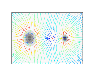
Figure 3. Streamlines for sink flow around a circle calculated by the adapted circle theorem for (a) no additional sink at the origin, and (b) an additional sink of equal strength placed at the origin. The black circles represent the radii of the plumes given by (2.5) at height  $z^{*}=0$. At this height, the lower plume has radius $R$ and the upper plume is a point source (not to scale). The stagnation point in (b) is marked with a red cross.
Upon addition of the second sink, the complex potentials in (3.8) and (3.9) become
 \begin{equation} \varOmega(Z) ={-}\frac{m_1}{2{\rm \pi}}\left[\ln(Z-\chi) - \ln(R^2/Z-\chi)\right] - \frac{m_2}{2{\rm \pi}}\ln Z \end{equation}
and
 \begin{equation} \varOmega(Z^{*}) ={-}\frac{m_2}{2{\rm \pi}}\ln\Bigg[\left(\frac{(Z^{*}-1)Z^{*}} {\gamma^2-Z^{*}}\right)^MZ^{*}\chi\Bigg], \end{equation}
respectively, where  $M=m_1/m_2$ is the ratio of sink strengths. The equation for the streamfunction changes similarly as
 \begin{align} \psi(x^{*},y^{*})
&={-}\frac{m_1}{2{\rm \pi}}\arctan\left(\frac{y^{*}(\gamma^2(2x^{*}-1)-(x^{*2}+y^{*2}))}{\gamma^2(x^{*}(x^{*}-1)-y^{*2})-x^{*}(x^{*2}+y^{*2})+x^{*2}+y^{*2}}\right)
\nonumber\\ &\quad - \frac{m_2}{2{\rm \pi}}
\arctan\left({\frac{y^{*}}{x^{*}}}\right).
\end{align}
\begin{align} \psi(x^{*},y^{*})
&={-}\frac{m_1}{2{\rm \pi}}\arctan\left(\frac{y^{*}(\gamma^2(2x^{*}-1)-(x^{*2}+y^{*2}))}{\gamma^2(x^{*}(x^{*}-1)-y^{*2})-x^{*}(x^{*2}+y^{*2})+x^{*2}+y^{*2}}\right)
\nonumber\\ &\quad - \frac{m_2}{2{\rm \pi}}
\arctan\left({\frac{y^{*}}{x^{*}}}\right).
\end{align}
An example with equal sink strengths ( $M=1$) is plotted in figure 3(b). The additional sink at the origin means that a greater proportion of the flow is now directed into the lower plume. As a result, a stagnation point forms between the two plumes and its position is controlled by the ratio of sink strengths $M$.
$M$.
As mentioned above, Coelho & Hunt (Reference Coelho and Hunt1989) also pointed out the similarity between an entraining jet or plume and a cylinder with suction at the surface. The method presented above (applying the modified circle theorem plus an additional sink to represent a circular sink of known strength) has applications for modelling other situations. One example would be the insertion of a porous cylinder into a two-dimensional flow for the purpose of extracting fluid. For example, a sink concentric with the circular boundary in figure 2(b) would have the effect of drawing some of the ambient flow into the cylinder, altering the flow field accordingly. If the additional sink were replaced by a source, that would alternatively represent fluid extrusion through a porous cylinder. Sucking or blowing at the boundary of cylindrical obstacles is one method of modifying fluid–structure interaction to reduce drag or to increase flow stability for instance (Fransson, Konieczny & Alfredsson Reference Fransson, Konieczny and Alfredsson2004; Chen et al. Reference Chen, Huang, Chen, Yu and Gao2022). It is possible that a suitable coordinate transformation may allow application of this method using the circle theorem to represent a sink of non-circular geometry (for example, this would be straightforward for an elliptical sink).
3.3. Entrainment in offset sources
To calculate the sink strengths at any given height, we take the sink strength to be equal to the entrainment across any velocity-potential contour, which is shown by the entrainment-flux integral calculations of Rooney (Reference Rooney2016). Since the entrainment constant  $\alpha$ is selected as in Morton et al. (Reference Morton, Taylor and Turner1956), the entrainment flux into the plume at any particular height is equivalent to the sink strength and is defined by (Kaye & Linden Reference Kaye and Linden2004)
 \begin{equation} m = 2{\rm \pi}\alpha b w. \end{equation}
 Up until height  $z=0$, the lower plume is assumed to be unaffected by the upper plume source. Therefore, it is axisymmetric and the total entrainment into its circular area at this height can be calculated simply with (3.16). The similarity solution of Morton et al. (Reference Morton, Taylor and Turner1956) implies that
 \begin{gather} b \sim \alpha z \end{gather}
 \begin{gather}w \sim \alpha^{{-}2/3}F^{1/3}z^{{-}1/3}, \end{gather}
where  $F$ is the buoyancy flux of the plume.
When a small height above the upper plume point source is considered, both plumes can be assumed to remain approximately axisymmetric (Li & Flynn Reference Li and Flynn2021). As the height above the plume source increases, the plumes will distort so that there is no single value of radius. However, in the region under consideration, this distortion is initially small (as will be evident from RANS results in later sections) and the plumes will be assumed to have a circular cross-section, the radius of which can be calculated by the similarity solution (2.5).
Using the subscripts  $1$ and $2$ to correspond to the values of the upper and lower plumes, respectively, the entrainment of the upper plume at a height $z$ above the upper plume is given as
 \begin{equation} m_1 \sim \alpha^{4/3}F_1^{1/3} z^{2/3}. \end{equation}
For a vertical offset of  $\zeta$, the entrainment of the lower plume at this height is
 \begin{equation} m_2 \sim \alpha^{4/3}F_2^{1/3}(z + \zeta)^{2/3}, \end{equation}
and, hence, the ratio of entrainment is
 \begin{equation} M = \left(\frac{F_1}{F_2}\right)^{1/3}\left(\frac{z }{z + \zeta }\right)^{2/3}. \end{equation}
This indicates that  $M$ is zero at $z=0$, i.e. at the level of the point source. Additionally, in an unstratified environment it is assumed that the buoyancy flux does not vary with height and, hence, the ratio $F_1/F_2$ at all heights $z$ is equal to the initial ratio of buoyancy fluxes for the two plumes, so $M \rightarrow (F_1/F_2)^{1/3}$ for large $z$.
$z$.
3.4. Flow speed on contours
From the complex potential in (3.14), the velocity field may be obtained as  $\text {d}{\varOmega }/\text {d}Z = U-\text {i}V$. For vertically offset plumes, this is
 \begin{align} \frac{\text{d}{\varOmega}}{\text{d}{Z}} &= \frac{1}{\chi}\frac{\text{d}{\varOmega}}{\text{d}{Z^{*}}} \end{align}
 \begin{align} &={-}\frac{m_2}{2{\rm \pi}\chi} \frac{(M+1)Z^{*2}-(\gamma^2(2M+1)+1)Z^{*}+(M+1)\gamma^2}{(Z^{*}-\gamma^2)(Z^{*}-1)Z^{*}}, \end{align}
so that
 \begin{equation} U ={-}\frac{m_2}{2{\rm \pi}\chi}\frac{N}{D} \text{,} \end{equation}
where
 \begin{align} N &= (M+1)[(\gamma^{2}+x^{*2}-y^{*2})(1-x^{*})(\gamma^{2}-x^{*})x^{*}] \nonumber\\ &\quad -x^{*2}(\gamma^{2}-x^{*})(1-x^{*})(\gamma^{2}(2M+1)+1)\nonumber\\ &\quad +y^{*2}(M+1)(\gamma^{2}+1-3x^{*})(\gamma^{2}+x^{*2}-y^{*2})\nonumber\\ &\quad -x^{*}y^{*2}(\gamma^{2}+1-3x^{*}) (\gamma^{2}(2M+1)+1)+ 2x^{*2}y^{*2}(M+1)(3x^{*}-2\gamma^{2}-2)\nonumber\\ &\quad +2x^{*}y^{*2}(M+1)(\gamma^{2}-y^{*2})-x^{*}y^{*2}(3x^{*}-2\gamma^{2}-2)(\gamma^{2}(2M+1)+1) \nonumber\\ &\quad -y^{*2}(\gamma^{2}(2M+1)+1)(\gamma^{2}-y^{*2}), \end{align}
 \begin{align} D &= x^{*2}\gamma^4 - 2x^{*3}\gamma^2(\gamma^2+1)+x^{*4}(1+4\gamma^2+\gamma^4)-2x^{*5}(\gamma^2+1)+x^{*6} \nonumber\\ &\quad+y^{*4}(\gamma^4+1)+ x^{*2}y^{*2}(3(x^{*2}+y^{*2})+2\gamma^2(\gamma^2+1)+2(\gamma^2+1)-4x^{*}(1+\gamma^2)) \nonumber\\ &\quad-2x^{*}y^{*4}(\gamma^2+1)-2\gamma^2x^{*}y^{*2}(\gamma^2+1)+y^{*2}(y^{*4}+\gamma^4). \end{align}
To find the position of the stagnation point between the two plumes at height  $z=0$, we note that the velocity component $V$ goes to zero along the line $y^{*}=0$ that connects the two plumes. Hence, the flow speed along this line is entirely in the $x$ direction and can be found by evaluating
 \begin{equation} U|_{y^{*}=0} = \frac{(M+1)(\gamma^2+x^{*2})-x^{*}(\gamma^2(2M+1)+1)}{x^{*}(x^{*}-1)(x^{*}-\gamma^2)}. \end{equation}
To find the non-dimensional distance of the stagnation point from the lower plume centreline  $x_{s}^{*}$, $U_{y^{*}=0}$ is set equal to zero and the equation is solved for $x^{*}$ to obtain
 \begin{equation} x^{*}_{s} = \frac{\gamma^2(2M+1)+1\pm \sqrt{(\gamma^2(2M+1)+1)^2 - 4\gamma^2(M+1)^2}}{2(M+1)}. \end{equation}
Physically, the stagnation point must lie between the two plumes, otherwise one plume would be forced to behave as a source rather than a sink. Additionally, the stagnation point is valid only when it lies outside of the radii of the plumes. The solution given by the negative square root of (3.28) lies inside the radius of the lower plume and can therefore be disregarded. If the stagnation point given by the positive square root also lies within the lower plume radius, then plume detrainment occurs. The limiting case is defined where the stagnation point lies at  $x^{*}_{s} = \gamma$, i.e. on the radius of the circular sink at the point closest to the upper plume source. This value can be substituted into the positive square root case of (3.28) to find the corresponding critical ratio of sink strengths $M_c$ as
 \begin{equation} M_c = \frac{1-\gamma}{2\gamma}. \end{equation}
The value  $M_c$ describes the maximum ratio of sink strengths that can be reached before detrainment of the lower plume occurs and the flow field becomes unrealistic. If $M \leqslant M_c$, the sink at the origin is sufficiently strong to overcome detrainment and the lower plume continues to act as a sink at all points on its boundary. In this case, a valid stagnation point forms and its position is given by taking the positive square root in (3.28). Letting $(M+1)^{-1} = \phi \leqslant 1$, then (3.28) may be rewritten as
 \begin{equation} x^{*}_{s} = \frac{\phi}{2} + \gamma^2 \left(1 - \frac{\phi}{2} \right) \pm \sqrt{ \left( \frac{\phi}{2} + \gamma^2 \left(1 - \frac{\phi}{2} \right) \right)^2 - \gamma^2 }, \end{equation}
which helps demonstrate that  $x^{*}_{s} \rightarrow 1$ as $M \rightarrow 0$.
When  $M>M_c$, there is no stagnation point and the flow from the lower plume is directed into the upper plume such that the lower plume will eventually be absorbed by the upper plume. This is more likely to occur if the upper plume is ‘stronger’ (has a greater buoyancy flux) than the lower plume. In this case, the lower plume cannot maintain its own structure. The model therefore indicates the conditions under which the lower plume loses its integrity, and detrains into the upper plume. It should be noted that, at and beyond this point, the model described here will no longer represent the plume flow structure, since the flow has undergone a qualitative change. Streamlines for examples of different sink strength ratios $M$ are shown in figure 4.

Figure 4. Streamlines calculated by the adapted circle theorem with an additional sink positioned at the origin and  $M_c = 2$. The ratio of sink strengths are (a) $M = 1$, (b) $M = 2$ and (c) $M = 3$. The stagnation point is marked with a red cross in (a,b), but does not exist outside of the plume boundaries in (c). Therefore, (c) depicts a flow field that would be unrealistic for merging offset plumes.
4. Numerical simulation
4.1. The governing equations
We used ANSYS Fluent Academic Research Mechanical and CFD Release 2020 R2 (ANSYS Inc., Canonsburg, PA, USA) to perform RANS simulations. The steady RANS equations for mass and momentum conservation in an incompressible fluid, solved in a three-dimensional Cartesian coordinate system are
 \begin{gather} \frac{\partial (\rho u_i)}{\partial x_i} = 0, \end{gather}
 \begin{gather}\frac{\partial (\rho u_i u_j)}{\partial x_j} ={-}\frac{\partial p}{\partial x_i} + \frac{\partial}{\partial x_j}\left(\tau_{ij} - \rho \overline{u^{\prime}_{i} u^{\prime}_{j}} \right) + (\rho - \rho_a) g_i, \end{gather}
where  $u_i$ are the mean velocity components, $u_i^\prime$ are the fluctuating velocity components, $p$ is pressure, $\rho$ is density, $\rho _a$ is ambient density and $g_i = (0,0,-g)$ in the $x$,
$x$,  $y$ and $z$ directions, where $g$ is the magnitude of acceleration due to gravity. The Reynolds stresses $\rho \overline {u^{\prime }_{i} u^{\prime }_{j}}$ are modelled using turbulence models to close the system of equations. The deviatoric stress tensor $\tau _{ij}$ is defined as
 \begin{equation} \tau_{ij} = \mu\left(\frac{\partial u_j}{\partial x_i} + \frac{\partial u_i}{\partial x_j}\right) - \frac{2}{3}\mu\frac{\partial u_k}{\partial x_k}\delta_{ij}, \end{equation}
where subscript  $i,j,k= 1,2\text { and }3$ and $\mu$ is dynamic viscosity.
Using the Boussinesq approximation, we assume small temperature differences and consider only density variations in the buoyancy term in the momentum equation
 \begin{equation} (\rho - \rho_a)g \approx{-}\rho_a\beta(T-T_a)g, \end{equation}
where  $\beta$ is the coefficient of thermal expansion, $T$ is a reference temperature and $T_a$ is the constant ambient temperature. Therefore, the density $\rho$ can be expressed as
 \begin{equation} \rho = \rho_a \left (1-\beta(T-T_a) \right ) . \end{equation}
 To close the system of equations, we use a  $k$-
$k$- $\epsilon$ turbulence model that is known to be robust in modelling a range of turbulent flows. In particular, we use the renormalisation group (RNG) $k$-
$k$- $\epsilon$ turbulence model, based on its success in modelling a single plume (Cook & Lomas Reference Cook and Lomas1998) and multiple plumes (e.g. Mokhtarzadeh-Dehghan et al. Reference Mokhtarzadeh-Dehghan, König and Robins2006; Durrani et al. Reference Durrani, Cook, McGuirk and Kaye2011). The turbulent kinetic energy $k$ and dissipation rate $\epsilon$ transport equations for the RNG $k$-
$k$- $\epsilon$ turbulence model are given as
 \begin{gather} \frac{\partial (\rho k u_i)}{\partial x_i} =\frac{\partial }{\partial x_j} \left(\alpha_k \mu_{t} \frac{\partial k }{\partial x_j} \right) +G_k +G_b - \rho \epsilon, \end{gather}
 \begin{gather}\frac{\partial (\rho \epsilon u_i)}{\partial x_i} =\frac{\partial }{\partial x_j} \left(\alpha_\epsilon \mu_{t} \frac{\partial \epsilon }{\partial x_j} \right) + C_{1\epsilon} \frac{\epsilon}{k}(G_k+ C_{3 \epsilon} G_b)- C_{2 \epsilon}^* \frac{\epsilon^2}{k} , \end{gather}
with turbulent viscosity  $\mu _t = \rho C_\mu k^2/\epsilon$. The inverse effective Prandtl numbers $\alpha _k$ and $\alpha _\epsilon$ correspond to the turbulent kinetic energy $k$ and dissipation rate $\epsilon$, respectively, and their values are obtained from the RNG theory by Orszag et al. (Reference Orszag, Yakhot, Flannery, Boysan, Choudhury, Maruzewski and Patel1993).
Here  $G_k$ is the generation of turbulent kinetic energy $k$ due to the mean velocity gradients and is defined as
 \begin{equation} G_k = \mu_t(2S_{ij}S_{ij})^{1/2} , \end{equation}
where the strain rate tensor  $S_{ij}$ is
 \begin{equation} S_{ij} = \frac{1}{2} \left( \frac{\partial{u_i}}{\partial{x_j}} + \frac{\partial{u_j}}{\partial{x_i}} \right) . \end{equation}
 The effect of buoyancy on turbulence was established to be significant by Nam & Bill (Reference Nam and Bill1993). Therefore, the generation of turbulent kinetic energy due to buoyancy  $G_b$ in (4.6) and (4.7) is modelled as
 \begin{equation} G_b = \beta g \frac{\mu_t}{\textit{Pr}_t} \frac{\partial T}{\partial x_i} , \end{equation}
with turbulent Prandtl number for energy  $\textit {Pr}_t = 0.85$.
The values for the model constants are  $C_{1\epsilon }=1.42$, $C_{2\epsilon }^*=2.0$ and $C_\mu =0.0845$. The constant that controls the effect of buoyancy in (4.7) is modelled according to Henkes, Van Der Vlugt & Hoogendoorn (Reference Henkes, Van Der Vlugt and Hoogendoorn1991) and is defined as
 \begin{equation} C_{3\epsilon} = \tanh{| v/u |}, \end{equation}
where  $v$ is the vertical velocity component parallel to the gravitational vector and $u$ is the horizontal velocity component perpendicular to the gravitational vector.
Finally, the energy transport equation is modelled as
 \begin{equation} \frac{\partial (\rho u_i h)}{\partial x_i} =\frac{\partial }{\partial x_j} \left[\left( \kappa + \frac{c_p \mu_t}{{\textit{Pr}}_t}\right) \frac{\partial T}{\partial x_j} \right] , \end{equation}
where the thermal conductivity  $\kappa =0.0248\ \text {W}\ (\text {m} \text {K})^{-1}$, specific heat capacity at constant pressure $c_p=1006.43 \text {J}\ (\text {kg}\ \text {K})^{-1}$ and $h$ is the specific enthalpy.
4.2. Computational domain and boundary conditions
A schematic of the computational domain and mesh for two vertically offset plume sources is shown in figure 5. The mesh shown is indicative of the Cartesian mesh used, but is much more coarse. Additionally, the actual source is much smaller compared with the domain, but was enlarged to make its geometry and the boundary conditions visible on the figure. To reduce the number of grids and computational complexity, we use an  $xz$ symmetry plane at $y=0$ and only model half of the plumes since the problem is symmetric about $y=0$. The two plumes are in close proximity to each other, therefore allowing for plume interaction in the domain. Both plumes have the same source length scale $d=0.02$ m, and the lower plume source is located at the bottom boundary $z= -\zeta$, where $\zeta$ is the vertical offset. To model the higher plume, we extrude a prism of dimensions $d \times d/2 \times \zeta$ from the base domain, which is located at a horizontal distance $\chi$ from the lower plume. The size of the domain measured in multiples of the plume source length scale is $30d\times 15d \times 50 d$ in the $x$,
$x$,  $y$ and $z$ directions, respectively. To prevent large-scale recirculation and instabilities, the size of the domain is relatively large compared with the length scale of the plume source. The horizontal extent of the domain in the $x$ direction of $30d$ is comparable to the set-up for two interacting plumes used by Durrani et al. (Reference Durrani, Cook, McGuirk and Kaye2011), where their domain is $40d$ in the $x$ and $y$ directions. Our domain has a ratio of $z_{max} / x_{max} =1.6$, which is similar to Pham, Plourde & Doan (Reference Pham, Plourde and Doan2007). We also ensured that the domain is high enough to allow the plumes to merge, thus preventing the influence of the top boundary conditions on the near-field region.

Figure 5. Computational domain and mesh with  $xz$ symmetry plane at $y=0$. The boundary conditions are colour coded. Grey, pressure inlet at ambient temperature for the bottom and side planes; red, pressure inlet at source temperature for plume sources; blue, pressure outlet for top plane; green, no-slip wall for plume offset. (Note: this is not to scale, the grid cells and plume sources have been scaled up for better visualisation)
Although the theory presented above assumes a point source, we can only model the plumes with a finite source. Therefore, we compare the results from both methods by estimating the virtual point source  $z_v$ of our plumes with finite sources. We model the plumes with square sources instead of a circular source because of the advantages of using a structured grid and the challenges associated with meshing in the case of a higher plume with a circular source inside a Cartesian domain. A structured grid provides a high level of quality and control for a mesh independence study, faster convergence because the elements are aligned to the flow, and lesser computational time due to less memory for storing mesh structure. Most importantly, if the source size is relatively small compared with the domain (as is the case for our set-up), the effect of source shape on the steady behaviour of an axisymmetric plume can be neglected because the cross-section quickly transitions to a circular cross-section, as observed by Marjanovic, Taub & Balachandar (Reference Marjanovic, Taub and Balachandar2017). In our simulations the cross-section becomes circular over heights of less than $3d$. Moreover, square sources in a Cartesian rectangular domain have been successfully used to model single axisymmetric plumes (e.g. Mokhtarzadeh-Dehghan et al. Reference Mokhtarzadeh-Dehghan, König and Robins2006; Yan Reference Yan2007; Marjanovic et al. Reference Marjanovic, Taub and Balachandar2017), and multiple axisymmetric plumes (e.g. Durrani et al. Reference Durrani, Cook, McGuirk and Kaye2011; Lou et al. Reference Lou, He, Jiang and Han2019).
The computational mesh is a structured grid with quadrilateral (two-dimensional) and hexahedral (three-dimensional) elements. A constant grid spacing  $\varDelta$ in the $x$ and $y$ directions and a stretched grid clustered at the sources with a growth rate of $1.02$ (i.e. $2\,\%$ increase in neighbouring cells) in the $z$ direction was implemented to capture the high turbulent kinetic energy that exists off-axis and away from the source (Pham et al. Reference Pham, Plourde and Doan2007). Table 1 provides the number of grid points $N_x$, $N_y$ and $N_z$ in the $x$,
$x$,  $y$ and $z$ directions for three different meshes used for the mesh independence study, which will be presented later. The details of the mesh used for all simulations are given under mesh M1 in table 1, where $\varDelta =0.1d$ in the $x$ and $y$ directions was found to be sufficient.
Table 1. Number of grid points  $N$ in $x, y$ and $z$ directions for three different meshes.

To closely model ‘interacting plumes’ in an unrestricted domain, we impose a Dirichlet boundary condition on the side, top and bottom boundaries, allowing for ambient fluid to enter at temperature  $T_a= 300\ {\rm K}$ and leave the domain. This was implemented using a pressure inlet boundary condition on the sides and bottom boundaries and imposing a pressure outlet condition on the top boundary. The sources were modelled using a pressure inlet condition at $T_0 = 800\ {\rm K}$, where $T_0>T_a$. Transition to turbulence occurs at about Grashof number $Gr\approx 10^9$ (Bill & Gebhart Reference Bill and Gebhart1975), where $Gr$ is defined as
 \begin{equation} Gr = { \left ( \frac{\mu_a}{\rho _a} \right ) } ^2 g z^3 \frac{(T_0-T_a)}{T_a}, \end{equation}
and  $\mu _a$ is the ambient dynamic viscosity.
Therefore,  $T_0$ is chosen such that the plume is turbulent relatively quickly at a height $z/\chi \approx 1$ in the computational domain. The gauge pressure for all boundaries was set to zero. A no-slip condition was imposed on the side walls of the higher plume source with length $\zeta$ for representing vertically offset plumes. The horizontal separation $\chi$ is such that the lower plume is unaffected by the no-slip side wall of the higher plume i.e. $z<0$, consistent with the assumption made in our analytical model.
4.3. Numerical method
The transport equations are discretised using a finite-volume-based method. A second-order upwind scheme was used for all convective terms. The least square method was used to compute the scalar values at the cell faces, velocity derivatives and secondary diffusion. We used the SIMPLE-consistent (SIMPLEC) scheme to solve the pressure–velocity coupling. A multigrid algorithm that computes corrections on a series of coarse grid levels was implemented to accelerate convergence. At the start of each simulation run, the entire domain was initialised to a temperature  $T=T_a + \delta {T}$ to improve convergence, where $\delta {T}$ is a small, uniform perturbation. The ratio $\delta {T}/T_a \approx 0.016$; however, the results were observed to be independent with respect to changes in $\delta T$. All simulations ran until the convergence criteria is satisfied, such that the residual of the conservation and transport equations is less than $10^{-5}$.
Since we only specify gauge pressure at the source and the source does not exhibit self-similarity, we calculate the dimensional source volume  $Q_0$, momentum $M_0$ and buoyancy $F_0$ fluxes by summing the flux of each grid cell at the square source, where the fluxes for each grid cell are defined as
 \begin{equation} Q_0= {\varDelta}^2 w, \quad M_0 = {\varDelta}^2w^{2}, \quad F_0 = {\varDelta}^2wg' , \end{equation}
and  $\varDelta =0.1d$ is the constant grid spacing.
Assuming the plume is axisymmetric and self-similar, we determine the dimensional fluxes at different heights above the source by integrating as follows:
 \begin{equation} \left.\begin{gathered} Q(z) = 2{\rm \pi}\int_{0}^{ \tilde{b}(z)} \tilde{w}(r,z)r \, \text{d}r, \quad M(z) = 2{\rm \pi}\int_{0}^{ \tilde{b}(z)} {\tilde{w}(r,z)}^2r \, \text{d}r, \\ F(z) = 2{\rm \pi}\int_{0}^{ \tilde{b}(z)} \tilde{w}(r,z) \widetilde{g'}(r,z)r \, \text{d}r . \end{gathered}\right\} \end{equation}
Here  $r$ is the radial coordinate relative to the local plume centre, and $\tilde {w}(r,z)$ and $\widetilde {g'}(r,z)$ correspond to the vertical velocity and buoyancy profiles, respectively.
The boundary conditions allow ambient fluid into the domain that leads to a component of vertical flow within the domain. Therefore, we only integrate within the plume by defining a plume radius  $\tilde {b}(z)$ to accurately quantify the fluxes. According to Cook & Lomas (Reference Cook and Lomas1998), the Gaussian plume radius $\tilde {b}(z)$ is estimated as the radial distance from the plume axis to the point at which the vertical velocity $\tilde {w}$ has fallen to $1/e$ of its axial value. We evaluate the accuracy of this approximation by comparing the volume flux $Q$ scaling with theory (Morton et al. Reference Morton, Taylor and Turner1956) in § 5.2. In the case of two interacting plumes, the flux for each independent plume is summed since we only compare results in the region where the plumes can be referred to as independent, as described by Cenedese & Linden (Reference Cenedese and Linden2014). Finally, to compare numerical results with theory, we use the approximation proposed by Cook (Reference Cook1998) that links the Gaussian profile to the top-hat profile
 \begin{equation} w = \tilde{w}_c/2, \quad b = \sqrt{2} \tilde{b}, \end{equation}
where  $\tilde {w}_c$ is the vertical centreline (peak) velocity of the Gaussian profile, and $w$ and $b$ are the top-hat velocity and top-hat radius, respectively.
5. Results
Simulations were performed at a fixed horizontal separation for a range of vertical offsets. To non-dimensionalise results, we take the characteristic length to be the horizontal source separation  $\chi = 0.2$ m, and the characteristic velocity is $(F_0/\chi )^{1/3}$. In this paper an asterisk is used to distinguish dimensional quantities from their dimensionless equivalents. We begin by simulating the single plume case to obtain the entrainment constant $\alpha$ and virtual origin $z_v$ used in the theory. We then verify the no offset case with existing theory and results. Finally, we extend the model to the case of vertically offset merging plumes described above, concentrating on the entrainment field at different heights in the region between the upper source and the initial merger of plumes. In order to compare the predictions made by the theoretical and numerical models in this paper, the virtual origin correction will be added into all heights from now on, i.e. we map $z \rightarrow z + z_v$.
5.1. Single plume
The source fluxes are estimated by summing the fluxes for each grid cell at the source using (4.14a–c). Therefore, the source volume  $Q_0$, momentum $M_0$ and buoyancy $F_0$ correspond to $1.21\times 10^{-4} \ \textrm {m}^3\ \textrm {s}^{-1}$, $3.73\times 10^{-5}\ \textrm {m}^4\ \textrm {s}^{-2}$ and $1.92\times 10^{-3}\ \textrm {m}^4\ \textrm {s}^{-3}$, respectively. The boundary conditions that impose the source fluxes lead to non-ideal conditions around the source, i.e. the plume around the source does not exhibit self-similarity. This behaviour can be characterised by the source parameter $\varGamma _0$ according to Hunt & Kaye (Reference Hunt and Kaye2001) as
 \begin{equation} \varGamma_0 = \frac{5Q_0^2F_0}{2^{7/2}\alpha {\rm \pi}^{1/2}M_0^{5/2}}. \end{equation}
 The behaviour of a plume close to the source depends on the balance between  $M_0$ and $F_0$. Excess momentum ( $\varGamma _0 <1$) is referred to as a forced plume, momentum deficit ( $\varGamma _0 >1$) is a lazy plume and $\varGamma _0 =1$ is a pure plume. Lazy and forced plumes tend toward a pure plume far field from the source, thus becoming self-similar away from the source. Based on the estimated source fluxes, we obtain a lazy plume of $\varGamma _0 = 6.77$, causing a narrowing of the plume radius $b$ close to the source over a distance of $4d$, which is close to the results of Marjanovic et al. (Reference Marjanovic, Taub and Balachandar2017).
The radial profiles of vertical velocity  $\tilde {w}$ and reduced gravity $\widetilde {g'}$ at two heights $z/d =15$ and $30$ above the source are presented in figure 6 where the $\tilde {w}$ and $\widetilde {g'}$ are non-dimensionalised by $F_0^{-1/3} z^{1/3}$ and $F_0^{-2/3} z^{5/3}$, respectively. The relative closeness of the radial curves at $z/d$ of $15$ and $30$ for both $\tilde {w}$ and $\widetilde {g'}$ shows the self-similar behaviour of the plume. They also show good comparison with direct numerical simulation (DNS) results by Marjanovic et al. (Reference Marjanovic, Taub and Balachandar2017) and experimental results by Rouse, Yih & Humphreys (Reference Rouse, Yih and Humphreys1952). However, there is a larger difference at the plume's centreline ( $x=0$). The velocity underpredicts both experimental and DNS results, showing about a $10\,\%$ error, while the reduced gravity slightly overpredicts the experimental results with about a $2\,\%$ error.

Figure 6. Gaussian profile showing self-similarity at  $z/d = 15$ and $30$, and compared with DNS results by Marjanovic et al. (Reference Marjanovic, Taub and Balachandar2017) and experimental results by Rouse et al. (Reference Rouse, Yih and Humphreys1952). (a) Reduced gravity $\widetilde {g'}$ radial profile. (b) Vertical velocity $\tilde {w}$ radial profile.
The most reliable method to estimate  $z_v$ according to Devenish, Rooney & Thomson (Reference Devenish, Rooney and Thomson2010) uses the centreline reduced gravity $\widetilde {g'}_c$ scaling defined as ${\widetilde {g'}_c}{}^{3/5} z = {\widetilde {g'}_c}{}^{3/5} z_v + c$. Therefore, the virtual origin can be estimated by the magnitude of the slope of ${\widetilde {g'}_c}{}^{3/5} z$ against ${\widetilde {g'}_c}{}^{3/5}$ in the fully developed region ( $\widetilde {g'}_c \sim z^{-5/3}$). Figure 7 shows the curve of ${\widetilde {g'}_c}{}^{3/5} z$ against ${\widetilde {g'}_c}{}^{3/5}$, and in the fully developed region, where ${\widetilde {g'}_c}{}^{3/5} < 3$, the equation of the line is given as
 \begin{equation} \widetilde{g'}_c z ={-}0.011\ \text{m}\ \widetilde{g'}_c + 0.365\ \text{m}. \end{equation}
Hence, the dimensionless virtual origin  $z^{*}_v=0.011/ \chi$ is 0.055. This value is used to represent the virtual origin of each plume in both the offset and no-offset cases to follow.

Figure 7. Virtual origin correction using centreline reduced gravity  $\widetilde {g'}_c$. Equation of the linear fit in the fully developed region is given as $\widetilde {g'}_c z = -0.011\ \textrm {m}\ \widetilde {g'}_c + 0.365\ \textrm {m}$.
According to the jet-length-based correction by Morton (Reference Morton1959), the virtual origin can be estimated as  $z_v = 1.057 L_m$, where $L_m$ is a momentum jet length defined as
 \begin{equation} L_m=2^{{-}5/4} \alpha^{{-}0.5} {\rm \pi}^{{-}1/4}\frac{M_0^{3/4}}{F_0 ^{1/2}}. \end{equation}
Based on their formulation, the dimensionless virtual origin  $z^{*}_v=0.053$ shows good agreement with our prediction from the reduced gravity scaling.
A mesh independence study was conducted using three meshes with varying grid points as shown in table 1. The centreline scaling of vertical velocity  $\tilde {w}_c$ and reduced gravity $\widetilde {g'}_c$ with $z^{*}$ are presented in figure 8 for the three meshes, and the $\tilde {w}_c$ and $\widetilde {g'}_c$ are non-dimensionalised by $F_0^{-1/3} \chi ^{1/3}$ and $F_0^{-2/3} \chi ^{5/3}$, respectively. The initial velocity increase is due to the non-ideal conditions (i.e. laziness) at the source. Away from the source, at $z^{*} > 1$, $\widetilde {g'}_c$ and $\tilde {w}_c$ approximately scale by $z^{*-5/3}$ and $z^{*-1/3}$, respectively, which is consistent with the scaling of turbulent plumes (Morton et al. Reference Morton, Taylor and Turner1956). Around the source, the meshes converge as the grid points increase from M3 to M1, thus showing mesh independence.

Figure 8. Mesh independence study showing the centreline scaling of the dimensionless  $\tilde {w}_c$ and $\widetilde {g'}_c$ with $z^{*}$ for three meshes. Here $\tilde {w}_c$ and $\widetilde {g'}_c$ scales by $z^{*-1/3}$ and $z^{*-5/3}$, respectively. The number of grid points increases from M3 to M1 with mesh details shown in table 1.
Based on the centreline velocity  $\tilde {w}_c$ where $r=0$, the constant value $C_w$ from the Gaussian profile of $\tilde {w}$ in (2.1) can be calculated to determine the vertical velocity scaling with height $z$. We express this as a top-hat velocity using (4.16a,b), therefore, the non-dimensionalised top-hat velocity $w^*$ scaling is
 \begin{equation} w^* = 1.92 {z^{*}}^{{-}1/3}. \end{equation}
 Entrainment is a key characteristic of a turbulent plume, and the entrainment constant  $\alpha$ is estimated using the same definition as given in Marjanovic et al. (Reference Marjanovic, Taub and Balachandar2017),
 \begin{equation} \alpha = \frac{\sqrt{2}\dfrac{\text{d}}{\text{d}z} \displaystyle\int\nolimits_{0}^{\tilde{b}} \tilde{w} r \, \text{d}r}{2 \left [\displaystyle\int\nolimits_{0}^{\tilde{b}} \tilde{w}^2 r \, \text{d}r \right]^{1/2} }. \end{equation}
 By computing (5.5) within the plume radius, the values of  $\alpha$ at different heights are shown in figure 9. We observe increasing entrainment as we move away from the source and as the plume approaches self-similarity. The entrainment variation with height becomes relatively constant ( $\alpha \approx 0.12$) in the self-similar/fully developed region, i.e. $z^{*} > 1$. The slight reduction in $\alpha$ at the top is attributed to the influence of the pressure outlet boundary condition; however, this is beyond the region of interest in the case of interacting plumes. The momentum deficit at the source leads to a lazy plume, causing an acceleration of the plume and increasing $\alpha$ before it becomes relatively constant in the self-similar region, as seen in figure 9. By contrast, the DNS results of Marjanovic et al. (Reference Marjanovic, Taub and Balachandar2017) show a larger value of $\alpha$ around the source region (as high as $0.2$) before it reduces, tending towards a constant $\alpha$. A possible reason for this could be that they use a different boundary condition for the source by specifying the source velocity, which will impose different flow behaviour in close proximity to the source. Another plausible reason for the lack of large entrainment near the source in our RANS simulation could indicate a limitation of the steady-state method in capturing the turbulent flow behaviour around the source, as discussed by Pham et al. (Reference Pham, Plourde and Doan2007). Although plumes exhibit variation in entrainment as seen here, we adopt a constant entrainment model for comparison with theory. We use the value of $\alpha$ in the self-similar region, i.e. $\alpha = 0.12$, which is within the range of $\alpha$ seen in the literature (e.g. Devenish et al. Reference Devenish, Rooney and Thomson2010; Marjanovic et al. Reference Marjanovic, Taub and Balachandar2017).

Figure 9. Variation of entrainment with height  $z^{*}$ by using (5.5) to estimate $\alpha$.
5.2. No vertical offset
When the plumes have no vertical offset, they will rise from point sources positioned at equal heights and the analytical model presented in this paper reduces to that of Rooney (Reference Rooney2016). Whilst it has been noted that the entrainment of each plume can affect the centreline velocity of its neighbour (Kaye & Linden Reference Kaye and Linden2004), the theoretical model neglects this deflection and takes the centreline separation as approximately constant and equal to  $\chi$ at all heights. The attraction of both plumes within the region of interest in the RANS simulation was observed to be small enough to justify its neglect.
The complex potential in (3.13) can be adapted to the case of no vertical offset by assuming that  $R \rightarrow 0$ such that the complex potential in terms of dimensionless quantity $Z^{*}$ becomes
 \begin{equation} \varOmega(Z^{*}) ={-}\frac{m_1}{2{\rm \pi}}\ln{(1-Z^{*})} - \frac{m_2}{2{\rm \pi}}\ln{( Z^{*}\chi)}, \end{equation}
and the streamfunction is given by
 \begin{equation} \psi(x^{*}, y^{*}) ={-}\frac{m_1}{2{\rm \pi}} \arctan\left(\frac{y^{*}}{x^{*}-1}\right) -\frac{m_2}{2{\rm \pi}}\arctan\left(\frac{y^{*}}{x^{*}}\right). \end{equation}
This is symmetric about the midpoint, so the plumes will have equal radii at any height. Hence, the equal strength plumes give a sink strength ratio  $M=1$ and, at any given height, the stagnation point lies directly between the two plumes at $x^{*}_{s} = 0.5$.
Contours of vertical velocity,  $w$, from the RANS simulation for two interacting plumes with no vertical offset are non-dimensionalised by a characteristic velocity $(F_0/\chi )^{1/3}$ and presented in figure 10. Initially there is relatively little deflection of the plumes from the vertical, but as they rise, the independent plumes attract and entrain each other, eventually merging to form a merged single plume far from the source (Baines Reference Baines1983). However, to compare both theory and numerical simulation, we only focus on the region before the plumes merge.

Figure 10. Contour plot of non-dimensional vertical velocity for two symmetric plumes with no vertical offset.
The variation of total volume flux  $Q^*$ with height $z^{*}$ for two interacting and non-interacting plumes are shown in figure 11. Here $Q$ is calculated for the interacting plumes by integrating across each of the independent plumes using (4.15), while the volume flux for the single plume set-up is doubled to obtain $Q$ for the non-interacting case. Since the $Q$ scaling for both results is similar, we conclude that two interacting plumes have little to no effect on the total volume flux within the region of interest, i.e. before the plumes start to merge. The results are compared with the equation for total volume flux carried by two plumes as defined by Cenedese & Linden (Reference Cenedese and Linden2014),
 \begin{equation} Q = 2\left ( \frac{9}{10} \right ) ^{1/3} \frac{6}{5} {\rm \pi}^{2/3} \alpha ^{4/3} F_0 ^{1/3} z^{5/3}. \end{equation}
Our result underestimates the total volume flux but has a similar scaling. The reason we underpredict the volume flux is attributed to the method of approximating the Gaussian radius  $\tilde {b}$ defining the region of integration. Nevertheless, this difference in flux is relatively small.

Figure 11. Non-dimensional total volume flux  $Q^*$ scaling from RANS simulations for two interacting and non-interacting plumes with no vertical offset, compared with Cenedese & Linden (Reference Cenedese and Linden2014) using (5.8). Here $Q$ is non-dimensionalised by $\chi ^{-5/3} F_0^{-1/3}$. The non-interacting result is twice the volume flux for a single plume.
Figure 12 shows the streamlines predicted by the numerical simulation at a height of  $z^{*}=0.75$ and coloured with a non-dimensional velocity magnitude of $u$ and $v$. Due to the respective entrainment of both plumes, a stagnation point $x^{*}_{s}$ forms between the plumes. The dimensionless vertical velocity contour across the plane further reveals the radii of the plumes to be slightly distorted due to the entrainment field. The stagnation point between the plumes is represented by the red cross at $x^{*}_{s} = 0.5$. The dimensionless horizontal velocity $u^{*} = u / (F_0/\chi )^{1/3}$ along the line $y^{*}=0$ is plotted for different heights in figure 13. As this is the horizontal velocity, flow towards the centre is positive at the left edge and negative at the right edge of each panel. Since the entrainment of each plume is of equal strength, the dimensionless horizontal velocity $u^{*}$ between the plumes will be negative when $x^{*}<0.5$ and positive when $x^{*}>0.5$. Therefore, a stagnation point exists where the velocity is zero, which occurs at $x^{*}=0.5$. The dimensionless centreline horizontal velocity predicted by the RANS simulation shows good agreement with the results of the theoretical model that are plotted in red alongside the RANS results in figures 13(b)–13(d). Each plume seeks to draw fluid in toward the plume axis through entrainment. As a result, the horizontal flow speeds between the two plumes are lower than those outside the plumes since the flow induced by the two plumes is acting in opposite directions.

Figure 12. The RANS streamlines on the  $xy$ plane at $z^{*} = 0.75$ for no vertical offset $\zeta ^{*}= 0$, coloured by the velocity magnitude and non-dimensionalised by the source velocity $(F_0 / \chi )^{1/3}$. The grey contours show the dimensionless vertical velocity $w^{*}$, and the red cross denotes the location of the stagnation point at $x^{*}_{s} = 0.5$.

Figure 13. (a) Dimensionless horizontal velocity  $u^{*}$ predicted by CFD simulation along $y^{*}=0$ for two plumes with no vertical offset. Comparison to the velocity predicted by the theoretical model (red) is shown for each of the heights $z^{*} = 0.5, 1.0$ and $1.5$ in (b–d), respectively. Shaded regions represent the area within the radius of each plume for which the theoretical model does not apply.
The dynamics of two merging plumes can be divided into three regions according to Cenedese & Linden (Reference Cenedese and Linden2014). The first region of the merging process, which is the focus of our work, is referred to as the independent region. The upper bound of this region is defined as the touching height  $z_t$, where the radius of the plumes touch. Using the top-hat formulation as defined in (4.16a,b), figure 14 plots the axes of the plumes at increasing heights, defined by the positions of maximum vertical velocity, and shows that the axes move inwards as the plumes interact. This indicates that the horizontal separation between plumes decreases with height, but this effect is small (less than 5 % of the horizontal separation $\chi$), and therefore validates the use of a constant horizontal separation in the theoretical model. The radii of both plumes at different heights are also plotted as data points. Our result is compared with the prediction of Cenedese & Linden (Reference Cenedese and Linden2014) taking mutual entrainment into account, and to the Morton et al. (Reference Morton, Taylor and Turner1956) model assuming no interaction. The touching height $z^{*}_t$ is obtained as the height where the radii coincide, i.e. $z^{*}_t=2.65$. Due to the inward movement of the plumes’ axes, the sum of the radii is $2b=0.92\chi$, which is less than the initial source separation. Cenedese & Linden (Reference Cenedese and Linden2014) predicted that $z^{*}_t = 0.35/\alpha$. By taking $\alpha =0.12$, as obtained from the single plume results earlier, $z^{*}_t=2.92$. Therefore, there is a $10\,\%$ difference compared with our results, which is relatively small. Assuming no interaction between the plumes (Morton et al. Reference Morton, Taylor and Turner1956), $z^{*}_t = 0.42/\alpha = 3.5$, which shows a larger difference of $32\,\%$ compared with our result.

Figure 14. Comparison of increasing the left and right plume radius  $b$ with height $z^{*}$ against Cenedese & Linden (Reference Cenedese and Linden2014) and Morton et al. (Reference Morton, Taylor and Turner1956). Inward movement of the plumes’ axes from the RANS case are shown, starting at $x^{*}=0$ and 1 for $z^{*}=0.5$. Plume axis is determined by the $x$ position of maximum $w$ velocity at a given $z^{*}$, while plumes radii $b$ is estimated using (4.16a,b).
Figure 13(a) appears to show two effects superimposed; a domain-wide convergence centred on the middle of the domain, with two local plumes converging on top. The implication of the horizontal velocity not going to zero at the points where the vertical velocity is maximum, as shown in figure 14, is that there may be a residual flow inside each local plume, which has the effect of reducing its lateral movement in the entrainment field. A qualitatively similar feature was discussed by Coelho & Hunt (Reference Coelho and Hunt1989), in the context of jet deflection being less than that of an equivalent solid body in a background current. (Internal plume circulations due to background flow are also evident in the data of Jordan et al. (Reference Jordan, Rooney, Devenish and van Reeuwijk2021) for instance.)
5.3. Vertically offset plumes
Figures 10 and 14 in the previous subsection show some evidence of plume distortion out of axisymmetry due to the effects of plume merging. The modelling of Rooney (Reference Rooney2016) and Li & Flynn (Reference Li and Flynn2021) accounts for this through the use of ‘generalized’ plume equations, which do not prescribe a simple shape for the horizontal plume cross-sections. This also requires specification of an entrainment assumption to close the system, which may then be integrated in the vertical ( $z$) direction to the point of merging and beyond.
One previous approach for modelling the internal properties of merging plumes has been simply to superimpose several, spatially offset copies of the trajectory and Gaussian profiles of a single plume, and sum up the fields within the plume boundaries (e.g. Davidson, Papps & Wood Reference Davidson, Papps and Wood1994; Yannopoulos Reference Yannopoulos2010). To examine the near field of merging offset plumes, we make the approximation here that, not far above the upper plume source, the plumes are similar to axisymmetric plumes. In particular, for each plume, the axisymmetric similarity solution gives both the radius and the entrainment. Hence, an approximation for the height evolution of  $M$ is obtained without the requirement for numerical integration of the generalized equations. This is a more approximate model than that of Rooney (Reference Rooney2016) and Li & Flynn (Reference Li and Flynn2021) and, unlike the ‘overlapping Gaussians’ approach, is not expected a priori to apply near to the point of merging (or beyond). The results presented below give an indication of the extent of its validity.
We investigate four vertical source offsets  $\zeta ^{*} = 0.25$, 0.5, $0.75$ and $1$ for a fixed horizontal source separation $\chi = 0.2$ m. Since we only consider the case where the two plumes have equal source fluxes, the value of $M$ in our experiments does not exceed $1$ such that $M \leqslant M_c$ and the theoretical model is valid for all considered configurations. We compare our results for heights $z^{*}\geq 0.5$ due to the ‘laziness’ of the simulated plume sources that leads to an initial acceleration of the buoyant fluid.
To obtain theoretical results with which to compare the RANS simulations, we require the entrainment constant  $\alpha$ and virtual origin $z_v$ calculated from the single plume as described previously. We assume both plumes have the same virtual origin. The radii of both plumes can subsequently be calculated from the similarity solution in (2.5), where the height $z$ takes into account $z_v$, i.e. $z \rightarrow z + z_v$.
From the equation for vertical velocity variation for a single plume given in (5.4), the non-dimensional top-hat vertical velocity  $w^*$ for the upper and lower plumes can be expressed as
 \begin{equation} w^*_1 = 1.92 z^{*-1/3} \quad \text{and} \quad w^*_2 = 1.92 (z^{*}+\zeta^{*})^{{-}1/3}, \end{equation}
respectively. Hence, the theoretical streamfunction in (3.15) can be calculated and used to find the velocity field components as
 \begin{equation} U = \frac{1}{\chi}\frac{\text{d}{\psi}}{\text{d}y^{*}} \quad \text{and} \quad V ={-}\frac{1}{\chi}\frac{\text{d}{\psi}}{\text{d}x^{*}}. \end{equation}
In each configuration the plumes were taken to have equal strengths such that the ratio of plume buoyancy fluxes is  $1$. Accounting for a virtual origin correction, the scaling of sink strength given in (3.21) can be adjusted for numerical simulation as
 \begin{equation} M = \left(\frac{z^{*}}{z^{*}+ \zeta^{*}}\right)^{2/3}. \end{equation}
Figure 15 validates this  $M$ scaling against the RANS simulation. The crosses represent the entrainment ratio $M$ predicted by the simulation at each height $z^{*}$, and each panel corresponds to a different vertical offset $\zeta ^{*}$. A line of best fit is plotted through the points for each offset, and the gradient of each line is very close to $1$, showing good agreement with the analytical solution (5.11).

Figure 15. The  $M$ scaling predicted by the analytical model is validated against the RANS simulation for different vertical offsets $\zeta ^{*}$. The crosses correspond to values of $M$ predicted by the simulation at heights $z^{*} \in \{0.5, 0.75, 1, 1.25, 1.5, 1.75, 2, 2.25, 2.5 \}$ above the numerical upper plume, and the dashed line represents a linear model fit to the data using ordinary least squares regression. All lines have a gradient equal to 1 when rounded to 8 decimal places.
Results obtained by the theoretical model can be further validated against RANS simulations. The first two rows of figure 16 give a comparison of the streamlines predicted by each method at two different heights. The cross-sections generated by the numerical simulation at heights  $z^{*} = 0.5$ and $z^{*} = 1.5$ are shown in figures 16(a) and 16(b), respectively. The plots show a greyscale contour plot of $w^{*}$ overlayed on the streamlines predicted by the simulation. The entrainment fields are similar to their theoretical equivalents in (c,d), and stagnation points form between the two plumes in each case. The entrainment flow field qualitatively agrees better between theory and RANS nearer the sources compared with higher up, as might be expected. Both stagnation points predicted by the theoretical model form closer to the lower plume, but the absolute error between predicted values is small: $0.012$ and $0.067$ for heights $z^{*} = 0.5$ and $z^{*} = 1.5$, respectively.

Figure 16. Results for two plumes with vertical source offset  $\zeta ^{*} = 0.75$ are taken from cross-sections of the $xy$ plane at heights $z^{*} = 0.5$ (a,c,e) and $z^{*} = 1.5$ (b,d,f). The first row shows a greyscale contour plot of $w^{*}$ overlayed on the streamlines predicted by the RANS solution, and the second shows the equivalent results predicted by the theoretical model. Stagnation points are marked with red crosses on the streamline plots in (a–d). Figures (e,f) show the velocity-potential contours produced by the theoretical model, where the grey shaded region represents the circular radii predicted by the similarity solution of Morton et al. (Reference Morton, Taylor and Turner1956).
The plume boundaries predicted by the radius similarity solution of Morton et al. (Reference Morton, Taylor and Turner1956), plotted as black circles in (c,d), are of a similar size to those predicted by the  $w^{*}$ contour plots generated by numerical simulation. The plumes exhibit a circular cross-section for $z^{*}=0.5$ with the lower plume having a larger radius. As the height above the plume source increases, the plume boundary deviates from a circular shape. This effect is also evident in the predictions of the theoretical model, as shown by the velocity-potential contour plots in figures 16(e) and 16(f). The circular radius predicted by the similarity solution of Morton et al. (Reference Morton, Taylor and Turner1956) is shaded in grey over contours of equal velocity potential. At height $z^{*}=0.5$, the circular radius aligns well with the plume radius predicted by velocity-potential contours. However, as the height increases, the plumes become more distorted and their boundaries less circular.
To obtain a quantitative comparison of theoretical and numerical results, we can compare the stagnation point position predicted between the two plumes. For the theoretical model, this is calculated by taking the positive square root in (3.28). To obtain the equivalent measurement from the numerical simulations, we find the position outside of the radii of the plumes along the  $x$ axis at which the velocity changes sign. Table 2 contains the locations of stagnation points predicted by each method for vertical offset $\zeta ^{*} = 0.25$. The numerical stagnation point is positioned closer to the upper plume than the theoretical stagnation point. Additionally, as the height above the upper plume is increased, the stagnation point moves towards the lower plume as the ratio of sink strengths $M$ increases. Similar observations were made for larger vertical offsets, and the average absolute error increased with an increase in the vertical offset.
Table 2. Comparison of the stagnation points predicted at different heights  $z^{*}$ above the numerical upper plume for vertical offset $\zeta ^{*} = 0.25$. The theoretical values are calculated by (3.28) and the ratio of sink strengths $M$ is given for each height.

Figure 17(a) shows example plots of the  $u^{*}$ velocity profiles along the line $y^{*}=0$ for a vertical offset $\zeta ^{*}=0.75$. The stagnation point $x^{*}_{s}$ moves towards the lower plume with increasing height; it is positioned at 0.643, 0.595 and 0.570 for $z^{*} = 0.5$, 1.0, and 1.5, respectively. We also see a domain-wide convergence and the presence of residual flow inside the plume, similar to the case of no vertical offset (figure 13). As in that case, these results are compared with the corresponding values of $u^{*}$ predicted by the theoretical model in figures 17(b)–17(d). These panels also show the prediction for equal-height plume sources from Rooney (Reference Rooney2016). That model assumes the same strength in all plumes, which is here taken as equal to that of the upper plume.

Figure 17. (a) Dimensionless horizontal velocity  $u^{*}$ from RANS simulation along $y^{*}=0$ for vertical offset $\zeta ^{*}=0.75$ is given at different heights $z^{*}$. Comparison to the velocity predicted by our theoretical model (red) is shown for each of the heights $z^{*} = 0.5, 1.0$ and $1.5$ in (b–d), respectively. This shows better agreement with RANS, particularly in the near field, in comparison with the model of Rooney (Reference Rooney2016) (blue).
Overall, the results exhibit good agreement and, although the comparison becomes worse as the height above the upper plume source is increased, the current theory shows a considerable improvement in the prediction of the near-field horizontal velocity between plumes when compared with the equal-height theory of Rooney (Reference Rooney2016). In particular, the equal-height theory becomes increasingly inaccurate as the vertical offset becomes larger, whilst the discrepancy of the proposed model remains small.
6. Conclusions
The results presented in previous sections show good correspondence between the analytical model and the results of RANS simulations. These two approaches represent different approximations to the real system. Their agreement provides encouragement for the use of these methods, while bearing in mind their possible limitations. In particular, we do not necessarily expect these methods to extend into the region of full merger without further development.
The model of Rooney (Reference Rooney2015, Reference Rooney2016) predicts that the cross-sections of merging plumes from point sources should distort out of circularity during merging. Figures 10 and 14 show evidence of this for plumes without vertical offset, in the asymmetry of plume profiles and in a touching height lower than that predicted by a non-interacting model, respectively. For offset plumes, the greyscale  $w^{*}$ contours in figure 16(a,b) shows that plume distortion is minimal at $z^{*}=0.5$ but more evident at $z^{*}=1.5$. This appears to be in broad agreement with that shown by the velocity-potential contours in figure 16(e,f), although the effect is less pronounced in the RANS results than in the analytical model. One possible reason for the difference may be that some internal plume circulation (discussed at the end of § 5.2) reduces deformation of the plume boundary. This is not yet allowed for in the analytical model, but could be an area for further development.
For the analytical model, the use of the axisymmetric similarity solution appears sufficient when the plumes are still approximately circular. However, at greater heights, it may be necessary to calculate the area etc. of the distorted plumes and solve the plume equations after the manner of Rooney (Reference Rooney2016) and Li & Flynn (Reference Li and Flynn2021) for example. This would also allow consideration of the effects of ambient stratification. Reynolds-averaged Navier–Stokes simulations may be challenged by the turbulent structures in the merging region, which is perhaps indicated here by the small variation of the estimated touching height compared with previous studies. Turbulence-resolving models could be used in future to obtain more detailed results. Time averaging such data over a long period would be required to examine entrainment flow, and this may present its own challenges (Devenish et al. Reference Devenish, Rooney and Thomson2010).
While there remains the potential for further work, the results and techniques herein have identified features of interest in the merger of offset plumes, as well as indicating that plume detrainment may occur in certain circumstances. As discussed above, the adapted circle theorem may also prove useful in the simulation of various other two-dimensional flows.
Acknowledgements
The authors would like to thank G. Keevil, A. Khan and S. Pegler for advising on different aspects of the project.
Funding
M.R., O.C., R.N., J.F. were supported in this work by the EPSRC-funded CDT in Fluid Dynamics, University of Leeds, grant EP/S022732/1. G.G.R. gratefully acknowledges the support of the Cheney Fellowship scheme at the University of Leeds. The numerical simulations were undertaken on ARC4, part of the High-Performance Computing facilities at the University of Leeds, UK.
Declaration of interests
The authors report no conflict of interest.


 Open access