


1. Introduction
The controlled production of tiny fluid entities such as drops, bubbles, emulsions and capsules has been extensively investigated over the last three decades because of its enormous relevance for a great variety of applications (Christopher & Anna Reference Christopher and Anna2007). In tip streaming (Montanero & Gañán-Calvo Reference Montanero and Gañán-Calvo2020) the dispersed phase is directed by some external actuation of either an electrical (Taylor Reference Taylor1964) or hydrodynamic nature (Suryo & Basaran Reference Suryo and Basaran2006) towards the tip of a suspended droplet (Eggleton, Tsai & Stebe Reference Eggleton, Tsai and Stebe2001) or fluid meniscus lifted above a fluid film (Cohen et al. Reference Cohen, Li, Hougland, Mrksich and Nagel2001) or attached to a feeding capillary (Zhang Reference Zhang2004). This tip emits quasi-monodisperse collections of drops/bubbles/emulsions either directly or through the breakage of a very thin jet. These fluid entities are smaller or even much smaller than any characteristic length of the microfluidic device. Tip streaming is frequently an elusive phenomenon, only found under particular conditions, which results from a delicate balance between the forces driving and opposing the flow (Montanero & Gañán-Calvo Reference Montanero and Gañán-Calvo2020).
Tip streaming can be produced by the hydrodynamic focusing caused by an outer stream moving faster than the dispersed phase when crossing a discharge orifice or tube. In this case, the drop of hydrostatic pressure and/or the viscous traction exerted by the outer stream collaborate in gently shaping a steady tapering meniscus to form a fluid converging ‘nozzle’. Tiny droplets can be directly ejected at the end of this fluid nozzle. Under certain conditions, the outer stream also sweeps away the capillary waves responsible for the breakup of the emitted fluid thread, thus allowing the formation of a thin jet (Huerre & Monkewitz Reference Huerre and Monkewitz1990). The jet eventually breaks up owing to the capillary instability (Rayleigh Reference Rayleigh1878), giving rise to a collection of droplets with an acceptable degree of monodispersity. Tip streaming is technologically advantageous even if that jet does not form because the droplets formed in the tip of the meniscus are still smaller than the characteristic length of the microfluidic device and exhibit a very high degree of monodispersity.
Several microfluidic configurations have been proposed to implement the hydrodynamic focusing principle in liquid–liquid systems. Figure 1 shows the main geometrical parameters governing the focusing effect. Table 1 shows the choices for those parameters leading to the different configurations: flow focusing (Gañán-Calvo & Riesco-Chueca Reference Gañán-Calvo and Riesco-Chueca2006), confined flow focusing (Cabezas et al. Reference Cabezas, Rubio, Rebollo-Muñoz, Herrada and Montanero2021), selective withdrawal (Cohen et al. Reference Cohen, Li, Hougland, Mrksich and Nagel2001), confined selective withdrawal (Evangelio, Campo-Cortés & Gordillo Reference Evangelio, Campo-Cortés and Gordillo2016), Raydrop (Dewandre et al. Reference Dewandre, Rivero-Rodriguez, Vitry, Sobac and Scheid2020), counter flow focusing (Utada et al. Reference Utada, Lorenceau, Link, Kaplan, Stone and Weitz2005) and opposed flow focusing (Dong et al. Reference Dong, Meissner, Faers, Eggers, Seddon and Royall2018). The focusing orifice/tube can be cylindrical or can have a converging shape, as indicated in the figure. The distance  $\hat {H}$ between the feeding capillary and the focusing orifice is a control parameter in all the configurations, which affects the flow stability and, therefore, the minimum size of the emitted droplets. We have coined the term ‘stretched flow focusing’ to refer to one of the two configurations studied in the present work. As can be observed, this geometry is a hybrid between flow focusing and confined selective withdrawal, in which the focusing effect is produced by a very long orifice or a very thick tube.

Figure 1. Microfluidic configurations based on the hydrodynamic flow focusing principle. The dashed line represents the nozzle used in confined flow focusing and counter flow focusing.
Table 1. Parameter relations corresponding to the microfluidic configurations which implement the hydrodynamic flow focusing principle. The last column indicates the shape of the focusing orifice.

Flow focusing (Gañán-Calvo & Riesco-Chueca Reference Gañán-Calvo and Riesco-Chueca2006) and confined selective withdrawal (Evangelio, Campo-Cortés & Gordillo Reference Evangelio, Campo-Cortés and Gordillo2015; Evangelio et al. Reference Evangelio, Campo-Cortés and Gordillo2016; Muñoz-Sánchez et al. Reference Muñoz-Sánchez, Silva, Pinho, Vega and Lima2016; He et al. Reference He, Campo-Cortés, Goral, López-León and Gordillo2019) are similar techniques to produce several microfluidic entities based on the hydrodynamic focusing principle. As shown in figure 1, the only difference between them is the shape of the discharge orifice located in front of the feeding capillary. While flow focusing uses an orifice located in a plate, the focusing effect in confined selective withdrawal is produced by a discharge tube. The applications of the axisymmetric liquid–liquid flow focusing configuration include the fabrication of flow cytometers (Lee et al. Reference Lee, Hung, Ke, Huang, Hwei and Lai2001), encapsulation and release of different actives (Takeuchi et al. Reference Takeuchi, Garstecki, Weibel and Whitesides2005; Utada et al. Reference Utada, Lorenceau, Link, Kaplan, Stone and Weitz2005; Sun et al. Reference Sun, Shum, Holtze and Weitz2010; Nabavi, Vladisavljevic & Manovic Reference Nabavi, Vladisavljevic and Manovic2017), and production of monodisperse cell-encapsulating microgel beads (Tsuda, Morimoto & Takeuchi Reference Tsuda, Morimoto and Takeuchi2010) and biodegradable poly(lactic acid) particles (Vladisavljevic et al. Reference Vladisavljevic, Henry, Duncanson, Shum and Weitz2012). Other applications are the fabrication of multiple emulsions as microreactors or fine templates for synthesizing advanced particles (Wang, Wang & Han Reference Wang, Wang and Han2011), single-step fabrication of multicompartment Janus microcapsules (Wu et al. Reference Wu, Yang, Liu, Xu, Zhu, Si and Xu2017), pesticide-loaded microcapsules (Zhong et al. Reference Zhong, Yang, Wu, Wang, Cheng, Dwivedi, Zhu, Si and Xu2020), as well as the production of polydimethylsiloxane (PDMS) microcapsules with tunable elastic properties (do Nascimento et al. Reference do Nascimento, Avendaño, Mehl, Moura, Carvalho and Duncanson2017) and multicompartment polymeric microcapsules (Wu et al. Reference Wu, Yang, Yang, Huang, Liu, Zhu, Si and Xu2018; Zhu et al. Reference Zhu, Wu, Han, Xu, Zhong, Yuan, Dwivedi, Si and Xu2018). The confined selective withdrawal geometry has been used to produce bubbles (Evangelio et al. Reference Evangelio, Campo-Cortés and Gordillo2015), emulsions (Evangelio et al. Reference Evangelio, Campo-Cortés and Gordillo2016), double emulsions and nematic shells (He et al. Reference He, Campo-Cortés, Goral, López-León and Gordillo2019), as well as micro-sized PDMS particles (Muñoz-Sánchez et al. Reference Muñoz-Sánchez, Silva, Pinho, Vega and Lima2016). Dewandre et al. (Reference Dewandre, Rivero-Rodriguez, Vitry, Sobac and Scheid2020) have recently engineered a new device, called Raydrop, with a vanishing disperse flow rate, and in which dripping to jetting transition was found as a function of the outer flow rate.
Both in flow focusing (Gañán-Calvo & Riesco-Chueca Reference Gañán-Calvo and Riesco-Chueca2006) and confined selective withdrawal (Evangelio et al. Reference Evangelio, Campo-Cortés and Gordillo2016), the size of the droplets produced via tip streaming critically depends on the ratio between the flow rates at which the inner (dispersed) and outer (continuous) phases are injected/withdrawn. In fact, the smallest droplets are always produced when the disperse-phase flow rate takes its smallest value compatible with the tip streaming stability (the so-called minimum flow rate stability limit) (Cabezas et al. Reference Cabezas, Rubio, Rebollo-Muñoz, Herrada and Montanero2021). This stability limit, in turn, is expected to depend on the specific geometry used to produce the hydrodynamic focusing. The role played by the geometrical parameters in the stability of the tapering meniscus is not well understood yet. Some studies have considered this problem in the gas–liquid flow focusing configuration (Vega et al. Reference Vega, Montanero, Herrada and Gañán-Calvo2010; Mu et al. Reference Mu, Qiao, Guo, Yang, Wu and Si2021). In the liquid–liquid case the results reduce to those of the experimental analysis by Evangelio et al. (Reference Evangelio, Campo-Cortés and Gordillo2016). In this paper we will study the influence of the hydrodynamic focusing geometry on both the tip streaming stability and size of the produced emulsions. Special attention will be paid to the distance  $\hat {H}$ between the feeding capillary and the discharge orifice/tube, which is probably the main control parameter of the microfluidic device. Another important aspect of the focusing geometry is the outer flow around the discharge orifice/tube. Pan, Nunes & Stone (Reference Pan, Nunes and Stone2020) have recently shown how the outer flow upstream of the tube's orifice affects the ratio of the two phases being withdrawn in selective withdrawal. In this work we will consider and compare both the flow focusing and confined selective withdrawal configurations.
Soluble surfactants play a fundamental role in many microfluidic applications (Anna Reference Anna2016). In hydrodynamic focusing the dispersed phase is injected or withdrawn from a reservoir at equilibrium with uniform monomer and micelle concentrations. Those concentrations are convected by the incompressible fluid particles, and they remain constant throughout most of the dispersed phase domain. The interface with the continuous phase constitutes a source/sink of surfactant molecules during the system evolution, and, therefore, spatial variations of surfactant concentration arise in the sublayer next to that surface. The adsorption/desorption kinetics and/or diffusion within the sublayer essentially govern the transfer of surfactant molecules from the bulk to the fresh interface created during the atomization. In hydrodynamic focusing the surfactant molecules adsorbed on the interface are convected towards the tip of the tapering liquid meniscus/film/droplet. The surface convection driven by the focusing stream can overcome the opposite Marangoni convection caused by the surface tension gradient. This results in the accumulation of surfactant molecules in the meniscus/film/droplet tip, which lowers the surface tension in that region, thus facilitating the tip streaming phenomenon. The effects of soluble surfactants on the tip streaming produced by hydrodynamic focusing have been studied in suspended droplets (De Bruijn Reference De Bruijn1993; Eggleton et al. Reference Eggleton, Tsai and Stebe2001) and bubbles (Booty & Siegel Reference Booty and Siegel2005) subject to extensional and shear flows, two-dimensional flow focusing (Anna, Bontoux & Stone Reference Anna, Bontoux and Stone2003; Lee, Walker & Anna Reference Lee, Walker and Anna2011) and selective withdrawal (Cohen Reference Cohen2004). To the best of our knowledge, this aspect of the problem has not yet being considered either in axisymmetric flow focusing or in confined selective withdrawal. In this paper we will examine the effect of soluble surfactants on both the stability of tip streaming and the size of the resulting droplets.
The calculation of the linear global modes (Theofilis Reference Theofilis2011) is an adequate tool to describe the instability mechanisms which limit the appearance of tip streaming. In this calculation one assumes that a long jet steadily tapers from the liquid meniscus and interrogates this basic flow about its response to small-amplitude perturbations (Sauter & Buggisch Reference Sauter and Buggisch2005; Tammisola, Lundell & Soderberg Reference Tammisola, Lundell and Soderberg2012; Gordillo, Sevilla & Campo-Cortés Reference Gordillo, Sevilla and Campo-Cortés2014; Cruz-Mazo et al. Reference Cruz-Mazo, Herrada, Gañán-Calvo and Montanero2017). If the largest growth rate of the eigenfrequency spectrum is positive, the jetting regime is unstable. In this case, one may analyse the interface perturbation amplitude of the eigenfunction responsible for the instability. If the amplitude almost vanishes in the tapering meniscus, the system is assumed to adopt a tip streaming mode, in which the droplets are produced right in front of the steady meniscus. On the contrary, if the amplitude is noticeable on the meniscus surface then we conclude that tip streaming does not occur. In this case, the growth of the unstable mode leads either to the interruption of the ejection or to self-sustained oscillations depending on the role played by the nonlinear terms. This paper will theoretically analyse the destabilizing mechanism when the dispersed phase flow rate is reduced just below the minimum flow rate stability limit. We will compare the predictions obtained from the global stability analysis with the experimental observations. The stability analysis will allow us to gain insight into the physical mechanisms responsible for the instability of the tip streaming in confined selective withdrawal.
2. Formulation of the problem
Consider the hydrodynamic focusing configuration sketched in figure 2. A liquid (the dispersed phase) of density  $\rho _i$ and viscosity $\mu _i$ is injected through a feeding capillary of radius $\hat {R}_c$ at a constant flow rate $Q_i$. The outer bath (the continuous phase) is another liquid of density $\rho _o$ and viscosity $\mu _o$ immiscible with the former. The dimensions of this bath are much larger than the rest of the lengths involved in the problem. The surface tension of the liquid–liquid interface in the absence of surfactant is $\gamma _0$. The two liquids are sucked at a constant flow rate $Q_s$ through a discharge tube of diameter $D$ and thickness $e$ placed at a distance ${\hat H}$ from the feeding capillary. The discharge tube is very long in terms of $D$, and, therefore, its length has little influence on both the stability of the tapering meniscus and the size of the emitted droplets. The above configuration corresponds to stretched flow focusing and confined selective withdrawal for $e\gg D$ and $e\lesssim D$, respectively. As explained below, monodisperse collections of droplets of diameter $\hat {d}$ are produced in the tip streaming modes of these configurations. When surfactants are added to one of the liquid phases, the formulation of the problem must be completed with the parameters characterizing the bulk diffusion of surfactant molecules, the adsorption–desorption kinetics at the interface and the dependency of surface tension upon the surface surfactant concentration. We do not introduce these parameters because this aspect of the problem will not be studied theoretically.

Figure 2. Sketch of the fluid configuration.
In the absence of surfactant, the problem can be formulated in terms of dimensionless geometrical parameters  $R_c=\hat {R}_c/D$, $H=\hat {H}/D$ and $\varepsilon =e/D$, the density and viscosity ratios $\rho =\rho _i/\rho _o$ and $\mu =\mu _i/\mu _o$, the Reynolds and capillary numbers,
 \begin{equation} \mbox{Re}=\frac{\rho_o U D}{\mu_o} \quad \text{and} \quad \mbox{Ca}=\frac{\mu_o U}{\gamma_0}, \end{equation}
where  $U=4 Q_s/({\rm \pi} D^{2})$ is the mean velocity in the discharge tube, and the flow rate ratio $Q=Q_i/Q_s$. As mentioned above, we consider experimental realizations in which $\varepsilon \gg 1$ and $\varepsilon \lesssim 1$, which corresponds to the stretched flow focusing and confined selective withdrawal configurations, respectively.
In the absence of surfactant, the mode adopted by the system, the droplet diameter  $d=\hat {d}/D$ and the droplet production frequency $f=\hat {f}D/U=3Q/(2d^{3})$ depend on the set of governing parameters $\{\varepsilon$, $R_c$, $H$;
$H$;  $\rho$, $\mu$, $\mbox {Re}$, $\mbox {Ca}$, $Q\}$. The density ratio $\rho$ takes values around unity in most liquid–liquid systems, and, therefore, it can be ruled out from the analysis. The dimensionless parameters $\mu$, $\mbox {Re}$ and $\mbox {Ca}$ vary when the outer viscosity changes in our experiments and simulations. To simplify the description of our results, we will categorize the simulations and experiments in terms of the outer viscosity or the viscosity ratio instead of the above-mentioned dimensionless numbers.
We distinguish the following flow modes: (i) jetting via tip streaming in which a jet is extruded from the tip of a steady liquid meniscus hanging on the feeding capillary (mode I), (ii) dripping via tip streaming (microdripping) in which droplets are periodically produced right in front of the tip of a steady meniscus (mode II), and (iii) unstable ejection in which the meniscus emits trains of droplets (modes IIIa and IIIb). As can be seen, and to simplify the analysis, experimental realizations are identified as modes I, II or III regardless of the size of the emitted jet or droplets. figure 3 shows examples of all these modes. As can be observed, only modes I and II lead to monodisperse collections of droplets.

Figure 3. Flow regimes: mode I (jetting), mode II (microdripping), modes IIIa and IIIb (intermittent ejection of drops trains).
3. Experimental method
The experimental set-up is sketched in figure 4. The focused (inner) and focusing (outer) liquids are withdrawn through a glass discharge tube (A) inserted into a transparent cell (B) across its bottom. The focused liquid is supplied through a sharpened steel capillary (C) around 300  $\mathrm {\mu }$m in inner diameter located in front of the discharge tube around 200 (450) $\mathrm {\mu }$m in inner (outer) diameter by using a high-precision orientation–translation system. The outer cell square section is 10 mm in width, more than 15 times the feeding capillary outer diameter (600 $\mathrm {\mu }$m). The cell is filled with the focusing liquid to form a reservoir open to the atmosphere. We withdraw the liquids with a syringe pump (KD Scientific Legato 210) (D). The dispersed phase is injected with another syringe pump (KD Scientific, KDS120) (E). The focusing liquid withdrawn from the cell is continuously replaced to keep the free surface level approximately constant.

Figure 4. Experimental set-up: glass discharge tube (A), transparent cell (B), steel capillary (C), syringe pumps (D,E), high-speed CMOS camera (F) and optical fibre (G).
We chose to suck the focusing liquid instead of pumping it (Evangelio et al. Reference Evangelio, Campo-Cortés and Gordillo2016) because this procedure allows for conveniently varying the control parameter  $\hat {H}$. However, the maximum value of the withdrawn flow rate $Q_s$ is limited by the maximum pressure drop of 1 bar across the discharge circuit. This limitation is minimized by reducing the length of that circuit. The alternative to this configuration is to close and seal the liquid bath so that we can impose an arbitrarily large positive gauge pressure to pump the outer liquid (Evangelio et al. Reference Evangelio, Campo-Cortés and Gordillo2016). This method has no limitation in terms of the pressure gradient driving the flow. However, it requires dissembling, re-assembling, re-aligning and re-sealing the experimental cell every time we change the distance $\hat {H}$.
Digital images of the fluid configuration were acquired using a high-speed CMOS camera (Photron, Fastcam SA5) (F), which allowed us to acquire images at  $10^{4}$ f.p.s. with an exposure time of 6.944 $\mathrm {\mu }$s. The camera was equipped with optical lenses with a magnification ranging from 1.92 to 4.71 $\mathrm {\mu }$m pixel $^{-1}$. The camera could be displaced horizontally and vertically using a triaxial translation stage to focus the interface. The fluid configuration was illuminated from the backside by cool white light provided by an optical fibre (G) connected to a light source. We also acquired images using an auxiliary CCD camera (not shown in figure 4) with an optical axis perpendicular to that of the CMOS camera to check that the capillaries were correctly aligned. All these elements were mounted on an optical table with a pneumatic anti-vibration isolation system, which prevents errors in determining the stability limits caused by finite-amplitude vibrations coming from the building.
We used distilled water as inner liquid and two silicone oils as outer (focusing) streams. Their properties are shown in table 2. The surface tension of the water–silicone oil interface was measured with the theoretical image fitting analysis (TIFA) method (Ferrera, Montanero & Cabezas Reference Ferrera, Montanero and Cabezas2007), while the density and viscosity were taken from the manufacturer's specifications.
Table 2. Properties of the working liquids at 25  $^{\circ }$C. $\gamma$ is the interfacial tension of the interface between distilled water and the corresponding liquid.

In each experimental run we fixed the flow rate  $Q_s$ at which the two liquids were suctioned. For 10-cSt silicone oil, we started the experiment by setting a dispersed phase flow rate $Q_i$ sufficiently high to establish the steady jetting regime (mode I). Then, this flow rate was progressively reduced until the meniscus became unstable (mode III). The images allowed us to determine whether microdripping (mode II) was established during the experimental run. For 100-cSt silicone oil, the outer flow rate was not sufficiently high to produce steady jetting. We started the experiment by setting a flow rate $Q_i$ sufficiently high to establish the microdrippng mode. Then, $Q_i$ was progressively reduced until the meniscus became unstable. In all the experiments the diameter $d$ of the ejected droplets was determined with pixel resolution. We verified that the optical distortion caused by the cell and discharge tube was negligible. To this end, we checked that there was good agreement between the droplet diameter measured from the image and that calculated from the inner flow rate and the frequency at which the drops were ejected.
4. Governing equations and numerical method
In this work we calculate the base flow and its eigenmodes in the absence of surfactant to explain some of the effects observed in the experiments. In this section we present the governing equations and the numerical method used to conduct the above-mentioned calculation. Here, all the variables are made dimensionless with the diameter  $D$ of the discharge tube, the mean velocity $U=4Q_s/({\rm \pi} D^{2})$ in that tube and the focusing liquid viscosity $\mu _o$. The dimensionless, axisymmetric, incompressible Navier–Stokes equations for the velocity $\boldsymbol {v}^{(k)}(r,z;t)$ and pressure $p^{(k)}(r,z;t)$ fields are
 $$\begin{gather} (ru^{(k)})_r+rw^{(k)}_z=0, \end{gather}$$
 $$\begin{gather}\rho^{\delta_{ki}} \mbox{Re}\, (u^{(k)}_t + u^{(k)} u^{(k)}_r+ w^{(k)} u^{(k)}_z)={-}p^{(k)}_r+\mu^{\delta_{ki}} (u^{(k)}_{rr}+(u^{(k)}/r)_r+u^{(k)}_{zz}), \end{gather}$$
 $$\begin{gather}\rho^{\delta_{ki}} \mbox{Re}\, (w^{(k)}_t + u^{(k)} w^{(k)}_r+ w^{(k)}w^{(k)}_z) ={-}p^{(k)}_z+\mu^{\delta_{ki}\,} (w^{(k)}_{rr}+w^{(k)}_r/r+w^{(k)}_{zz}), \end{gather}$$
where  $t$ is the time, $r$ (
$r$ ( $z$) is the radial (axial) coordinate, $u^{(k)}$ ( $w^{(k)}$) is the radial (axial) velocity component and $\delta _{ij}$ is the Kronecker delta. In the above equations and henceforth, the superscripts $k=i$ and $o$ refer to the inner (disperse) and outer (continuous) phases, respectively. In addition, the subscripts $t$,
$t$,  $r$ and $z$ denote the partial derivatives with respect to the corresponding variables. The action of the gravitational field has been neglected due to the smallness of the fluid configuration.
The kinematic compatibility and the velocity field continuity at the interface  $r=F(z,t)$ yields
 \begin{equation} {F_t+F_z w^{(i)}-u^{(i)}=0, \quad u^{(i)}=u^{(o)}, \quad w^{(i)}=w^{(o)}.} \end{equation}
The equilibrium of both tangential and normal stresses on that surface leads to
 $$\begin{gather} \mu[(1-F_z^{2})(w^{(i)}_r+u^{(i)}_z)+2F_z(u^{(i)}_r-w^{(i)}_z)] =(1-F_z^{2})(w^{(o)}_r+u^{(o)}_z)+2F_z(u^{(o)}_r-w^{(o)}_z), \end{gather}$$
 $$\begin{gather} p^{(i)}+\mbox{Ca}^{{-}1}\frac{FF_{zz}-1-F_z^{2}}{F(1+F_z^{2})^{3/2}}-\frac{2\mu[u^{(i)}_r-F_z(w^{(i)}_r+u^{(i)}_z)+F_z^{2}w^{(i)}_z]}{1+F_z^{2}} \nonumber\\= p^{(o)}-\frac{2u[u^{(o)}_r-F_z(w^{(o)}_r+u^{(o)}_z)+F_z^{2}w^{(o)}_z]}{1+F_z^{2}}. \end{gather}$$
 We integrate the Navier–Stokes equations in the numerical domain sketched in figure 5. The red lines correspond to the contours of the feeding capillary and discharge tube used in the experiments of confined selective withdrawal, while the blue and black lines have been added to close the numerical domain. The cylindrical shape of the outer cylinder has a negligible influence on the results given the large distance between the cylinder wall and the interface. The discharge tube length is equal to  $2H$, and the feeding capillary length is $H$. The feeding capillary end is assumed to be infinitely thin to facilitate the numerical calculations, which may constitute a significant difference with respect to the experiments. The edge of the discharge tube has been rounded to eliminate numerical singularities associated with the vertex.

Figure 5. Sketch of the computational domain.
We impose a parabolic velocity distribution at the inlet section of the feeding capillary. A uniform velocity profile is prescribed on the lateral surface of the outer cylinder. The constant pressure and  $F_z=0$ conditions are imposed at the outlet section (the pressure in the inner phase equals the pressure in the outer phase plus the capillary pressure). The non-slip boundary condition is prescribed at the solid walls (red and blue lines in figure 5). The anchorage condition of the triple contact line, $F=1$, is prescribed at the edge of the feeding capillary. We impose the standard regularity conditions $u^{(i)}=w^{(i)}_r =0$ at the symmetry axis.
To calculate the linear global modes, we assume the temporal dependence
 \begin{equation} \left. \begin{aligned} U(r,z;t) & =U_0(r,z)+\delta U(r,z)\, {\rm e}^{-{\rm i}\omega t} \quad (\delta U\ll U), \\ F(z;t) & =F_0(z)+\delta F(z)\, {\rm e}^{-{\rm i}\omega t} (\delta F\ll F_0), \end{aligned} \right\} \end{equation}
where  $U(r,z;t)$ represents the velocity and pressure fields, $U_0(r,z)$ and $\delta U(r,z)$ stand for the base flow (steady) solution and the spatial dependence of the eigenmode, respectively, while $\omega =\omega _r+\textrm {i}\omega _i$ is the eigenfrequency characterizing the perturbation evolution. Special attention will be paid to the perturbation amplitude $\delta F(z)$ of the interface position $F(z;t)$ around the base flow solution $F_0(z)$. If the growth rate $\omega _i$ of the dominant mode (i.e. that with the largest $\omega _i$) is positive then the base flow is asymptotically unstable under small-amplitude perturbations (Theofilis Reference Theofilis2011). In this work we will determine the critical value of the flow rate ratio $Q$ for which the base becomes asymptotically unstable as a function of the rest of the governing parameters.
The growth of the linear perturbations makes the system enter into the nonlinear regime. The nonlinear terms of the Navier–Stokes equations and interface boundary conditions may stabilize the system. In this case, self-sustained oscillations, continuously fed by the growth of unstable infinitesimal perturbations, can be observed. Otherwise, the linear instability of the jetting (mode I) base flow is assumed to lead either to the microdripping mode (mode II) or intermittent liquid ejection (mode III). The outcome adopted by the system cannot be predicted from the linear stability analysis.
The governing equations are integrated with the numerical method proposed by Herrada & Montanero (Reference Herrada and Montanero2016). In this method the inner and outer fluid domains are mapped onto fixed numerical domains through a non-singular mapping with a quasi-elliptic transformation (Dimakopoulos & Tsamopoulos Reference Dimakopoulos and Tsamopoulos2003). The equations expressed in terms of  $t$ and the transformed spatial coordinates are discretized in the mapped radial direction with Chebyshev spectral collocation points (Khorrami, Malik & Ash Reference Khorrami, Malik and Ash1989). Fourth-order finite differences with equally spaced points are used to discretize the mapped axial direction.
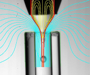
The accurate calculation of the dominant mode eigenvalue at the marginal stability demands very fine meshes, probably due to the complex base flow arising at the stability limit. In fact, and as will be shown in § 6, large velocity gradients can be found next to the interface. The resulting viscous forces affect the focusing stability and, therefore, must be accurately calculated to determine the critical conditions. It is worth noting that the minimum jet diameter was 6  $\mathrm {\mu }$m, around 50 times smaller than the inner diameter of the feeding capillary. We tried different grid configurations with different numbers of domains. The configuration shown in figure 6 was the only one producing good convergence. In this sense, the simulation is not a straightforward extension of that recently used for the confined flow focusing configuration (Cabezas et al. Reference Cabezas, Rubio, Rebollo-Muñoz, Herrada and Montanero2021). We verified that the results did not significantly depend on the mesh size. For instance, for $\{\varepsilon =0.59$, $R_c=1.69$, $H=1.66$; $\rho =1.07$, $\mu =0.107$; $\mbox {Re}=11.8$, $\mbox {Ca}=0.15$, $Q=0.059\}$, an increase of 40 % in the number of points produced errors in the critical flow rate ratio below 5 %. In each simulation the outer domain radius is selected so that the meniscus interface remains in the grid's cyan domain of figure 6. That value ranged from 4 to 7.5 times that of feeding capillary. We verified that the solution did not significantly depend on this choice. We also verified that the minimum flow rate ratio and the jet diameter did not depend on the cut-off length of the numerical domain. More precisely, a variation of 50 % of the discharge tube length produced a difference smaller than 0.5 % and 1.5 % in the minimum flow rate and the jet diameter, respectively.

Figure 6. Details of the grid used in the simulations. The grid consists of four blocks corresponding to the inner liquid (red) and the outer stream (cyan, green and magenta). Panel (b) shows details of the grid around the edge of the discharge tube.
5. Experimental results
This section presents experimental results on the stability of confined selective withdrawal and the diameter of the produced droplets in tip streaming realizations. We consider as a tip streaming realization that in which a steady liquid meniscus periodically emits droplets, regardless of whether a jet is formed in the discharge tube (mode I, jetting) or the droplets are ejected from the meniscus tip (mode II, microdripping). In our experiments with  $\mu =0.1$ (10-cSt silicone oil), tip streaming ejections were produced via the jetting and microdripping regimes. However, the jetting regime was not observed for $\mu =0.01$ (100-cSt silicone oil) due to the limited speed of the jet in the discharge tube, which makes the jet absolutely unstable (Huerre & Monkewitz Reference Huerre and Monkewitz1990).
In the jetting regime the droplet diameter can be estimated from that of the precursor jet by considering the wavelength of the most unstable capillary mode (Tomotika Reference Tomotika1936). In turn, the jet diameter can be estimated from continuity arguments in terms of the flow rate ratio. The dependence of the droplet diameter on the flow rate ratio in the microdripping mode is analysed for  $\mu =0.01$ in figure 7. The power law that best fits the experimental data is $d=1.14\, Q^{0.45}$. As can be observed, the experimental results are also accurately fitted by the law $d=1.35\, Q^{1/2}$, which leads to the production frequency $f=0.61 Q^{-1/2}$. Interestingly, the reduction of the flow rate ratio in the microdripping mode does not affect the shape of the tapering meniscus (figure 8). The meniscus tip sharpens as $Q$ decreases, which lowers the size of the droplets ejected in that region. The scaling law reported here is the same as that obtained by Evangelio et al. (Reference Evangelio, Campo-Cortés and Gordillo2016) for both the microdripping (short jets) and jetting (long jets) modes. In that work, the authors rationalize their experimental observations using arguments based on mass conservation. The collection of produced droplets exhibits a high degree of monodispersity. The standard deviation of the drop diameter is below 10 % in all the cases.

Figure 7. Drop diameter  $d$ vs the flow rate ratio $Q$ in the absence of surfactant for $\varepsilon =0.52$, $R_c=1.7$, $H=2.9$, $\rho =1.03$, $\mu =0.010$, $\mbox {Re}=0.40$ and $Ca=0.53$. The symbols and the solid line correspond to the experimental results and the scaling law $d=1.35\, Q^{1/2}$, respectively.

Figure 8. Images acquired for (a)  $Q=0.042$ and (b) $Q=0.001$. The rest of the governing parameters are the same as those in figure 7. The yellow line in the image (b) is the meniscus contour in case (a).
In this work we pay special attention to the influence on the flow stability and droplet diameter of two factors of the problem not systematically studied in previous works: (i) the geometry of the microfluidic configuration through the parameters  $H$ and $\varepsilon$, and (ii) the role played by the surfactant monolayer formed on the interface when a soluble surfactant is added to the inner liquid.
5.1. Influence of the feeding capillary-to-discharge tube distance
figure 9 shows the minimum value of the flow rate ratio,  $Q_{{min}}$, as a function of the capillary number $\mbox {Ca}$ for the smallest value of the viscosity ratio $\mu =0.01$ considered in our experiments. We conducted the experiments for three values of the distance $H$ between the feeding capillary and the discharge tube. For flow rate ratios larger than $Q_{{min}}$, the system adopts the microdripping regime (mode II), while unsteady ejection (mode III) is produced otherwise. The force driving the inner liquid ejection increases with the capillary number, stabilizing the tapering meniscus and increasing the range of $Q$ for which microdripping is obtained. There is a significant influence of the distance $H$ on the system stability for small values of $\mbox {Ca}$. However, this distance becomes irrelevant as the capillary number increases. In fact, the microdripping mode destabilizes for $Q\lesssim 10^{-3}$ regardless of the $\mbox {Ca}$ and $H$ values. Unfortunately, and due to the limitations of our experimental set-up, we could not analyse the system stability for $\mbox {Ca}\gtrsim 0.63$. As $H$ decreases, the stress exerted by the outer stream on the inner liquid increases, which stabilizes the liquid ejection in most cases. However, the dependence of $Q_{{min}}$ on $H$ is non-monotonic for some values of $\mbox {Ca}$.

Figure 9. Minimum value of the flow rate ratio,  $Q_{{min}}$, vs the capillary number, $\mbox {Ca}$, in the absence of surfactant for $\varepsilon =0.64$, $R_c=1.75$, $\rho =1.03$, $\mu =0.010$, and different values of the distance $H$ between the feeding capillary and the discharge tube. The Reynolds number took values smaller than 0.5.
The role played by  $H$ in the meniscus stability for a fixed value of $\mbox {Ca}$ is analysed in figure 10. As mentioned above, this parameter becomes irrelevant for the largest value of $\mbox {Ca}$ considered in our experiments. For $\mbox {Ca}=0.22$, the meniscus stabilizes as $H$ decreases. However, the diameter of droplets ejected in the microdripping mode depends only slightly on $Q$ at the stability limit. Therefore, the distance $H$ considerably affects the ejection frequency but not the droplet diameter. This is a reminiscence of the behaviour in quasi-static dripping, which takes place for a small disperse flow rate. For $H\simeq 0.5$ and $\mbox {Ca}=0.63$, we observe an instability mechanism consisting in the depinning of the triple contact line from the edge of the feeding capillary. In this case, the contact line climbs on the inner wall of the feeding capillary and remains still at a certain distance from the capillary end. This phenomenon is associated with the large extensional stress exerted by the viscous outer stream for small $H$, and has also been observed in similar configurations, such as gaseous flow focusing of viscoelastic jets (Ponce-Torres et al. Reference Ponce-Torres, Montanero, Vega and Gañán-Calvo2016). For $H\gtrsim 4.5$ and $\mbox {Ca}=0.22$, the triple contact line climbs on the outer wall of the feeding capillary. This occurs because the contact angle reaches the threshold value leading to the contact line depinning at the outer edge of the feeding capillary end. When the triple contact line is depinned, the system behaviour downstream is essentially the same as that taking place with pinned contact lines: if the flow rate ratio is greater/smaller than the critical one, then mode II/III is obtained. The tapering meniscus became unstable for $H\lesssim 2$ and $\mbox {Ca}=0.22$. As can be observed in figure 10, the sharp decrease of $Q_{{min}}$ when $\mbox {Ca}$ is increased translates into a reduction of one order of magnitude of the droplet diameter $d_{{min}}$ at the stability limit.

Figure 10. Minimum value of the flow rate ratio,  $Q_{{min}}$ (a), and the corresponding droplet diameter, $d_{{min}}$ (b), vs the distance $H$ between the feeding capillary and the discharge tube in the absence of surfactant for $\varepsilon =0.64$, $R_c=1.85$, $\rho =1.03$, $\mu =0.010$, and different values of $\mbox {Ca}$ and $\mbox {Re}$. For $H\simeq 0.5$ and $\mbox {Ca}=0.63$, the triple contact line climbs on the inner wall of the feeding capillary (open symbols). For $H\gtrsim 4.5$ and $\mbox {Ca}=0.22$, the triple contact line climbs on the outer wall of the feeding capillary (open symbols). The dashed line is a guide to the eye.
When the outer liquid viscosity  $\mu _o$ is reduced, the suction flow rate $Q_s$ must be increased to produce tip streaming. As a consequence, the outer liquid speed in the discharge tube increases, and so does the velocity of the liquid thread ejected by the meniscus tip. This allows the system to sweep away the capillary waves growing on the thread surface (convective instability) (Huerre & Monkewitz Reference Huerre and Monkewitz1990), and the jetting regime (mode I) can be produced. Thus, for $\mu =0.107$ and $Q>Q_{{min}}$, steady jetting was found in most of our experiments, while (as mentioned above) microdripping was always obtained for $\mu =0.010$. This occurred due to the limited outer flow rate produced by our experimental set-up for the high outer viscosity case. In fact, for a given suction flow rate, the jetting regime is more likely to occur for higher outer viscosity.
To fix the capillary and Reynolds numbers, one must fix the outer viscosity and total (suction) flow rate. Then, one must change the inner viscosity and inner flow rate so that the dependency of the critical flow rate ratio on the viscosity ratio can be analysed. The inner viscosity cannot be significantly reduced below that of water. Therefore, the only possibility is to use a viscous outer bath (e.g. 100 cSt silicone oil) and inner liquids with viscosities in the range, say, 1–10 cSt. In this case, the system is so viscous that the jetting regime cannot be produced with our experimental configuration, as explained above. For this reason, we considered water as the inner liquid and changed the bath viscosity. Unfortunately, this implies that the Reynolds and capillary numbers cannot be fixed simultaneously.
The comparison between the minimum flow rates measured for  $\mu =0.010$ and 0.107 (figure 11) shows that there is a significant interval of $H$ within which the outer viscosity hardly affects the stability limit (it must be noted that the Reynolds and capillary numbers did not take the same values for the two cases). However, the droplet diameter was considerably smaller in the lesser viscous case because those droplets were produced in the jetting regime.

Figure 11. Minimum value of the flow rate ratio,  $Q_{{min}}$ (a), and the corresponding droplet diameter, $d_{{min}}$ (b), vs the distance $H$ between the feeding capillary and the discharge tube in the absence of surfactant for $\varepsilon =0.62$ and $R_c=1.7$. The black symbols correspond to $\rho =1.03$, $\mu =0.010$, $\mbox {Ca}=0.22$ and $\mbox {Re}=0.15$, while the blue symbols correspond to $\rho =1.07$, $\mu =0.107$, $\mbox {Ca}=0.15$ and $\mbox {Re}=12$. For $H\lesssim 0.7$ and $\mbox {Ca}=0.15$, the triple contact line climbs on the inner wall of the feeding capillary (open symbols). For $H\gtrsim 4.5$ and $\mbox {Ca}=0.22$, the triple contact line climbs on the outer wall of the feeding capillary (open symbols). The dashed line is a guide to the eye.
5.2. Confined selective withdrawal vs stretched flow focusing
In confined selective withdrawal a tube with a thickness smaller than or similar to the tube diameter ( $\varepsilon \lesssim 1$) is placed in front of the feeding capillary to focus the inner liquid current and to collect the jet/droplets ejected by the tapering meniscus. When the tube thickness is much larger than the diameter ( $\varepsilon \gg 1$), the outer flow streamlines considerably change in the focusing region, which may significantly affect the outcome of the process. We conducted experiments with a very thick discharge tube to investigate this possible effect. As mentioned in the introduction, we have coined the expression ‘stretched flow focusing’ to refer to this configuration, which can be regarded as a hybrid between confined selective withdrawal and flow focusing.
figure 12 shows the minimum value of the flow rate ratio and the corresponding droplet diameter obtained for  $\mu =0.01$ with both the confined selective withdrawal and stretched flow focusing configurations. As can be observed, confined selective withdrawal considerably enhances the stability of the microdripping mode by reducing the minimum value of the flow rate ratio and by enlarging the interval of $H$ within which microdripping is produced. In fact, stable ejection was obtained with stretched flow focusing only for $2\lesssim H\lesssim 3$ when the capillary number was reduced to 0.22. For $\mbox {Ca}=0.63$ and $H\lesssim 1$, the meniscus became unstable in the stretched flow focusing configuration. The decrease of $Q_{{min}}$ achieved by confined selective withdrawal entails a significant reduction of the minimum value of the droplet diameter (figure 12b). The comparison between the images (a) and (b) in figure 13 shows that the upwards flow of the outer liquid around the discharge tube reduces the volume of the tapering meniscus and stretches the liquid thread formed at its tip. This effect seems to be responsible for the meniscus stabilization in confined selective withdrawal and allows one to reduce the droplet diameter by lowering the inner flow rate (figure 13c).

Figure 12. Minimum value of the flow rate ratio,  $Q_{{min}}$ (a), and the corresponding droplet diameter, $d_{{min}}$ (b), vs the distance $H$ between the feeding capillary and the discharge tube in the absence of surfactant for $\varepsilon =0.64$ (confined selective withdrawal) (squares) and $\varepsilon =22.2$ (stretched flow focusing) (triangles). The black and red symbols correspond to ( $Ca=0.63$, $Re=0.41$) and ( $\mbox {Ca}=0.22$, $Re=0.15$), respectively. The rest of the governing parameters are $R_c=1.8$, $\rho =1.03$ and $\mu =0.010$. For $H\lesssim 0.5$ and $\mbox {Ca}=0.63$, the triple contact line climbs on the inner wall of the feeding capillary in the confined selective withdrawal configuration. For $H\gtrsim 4.5$ and $\mbox {Ca}=0.22$, the triple contact line climbs on the outer wall of the feeding capillary in the confined selective withdrawal configuration.

Figure 13. Images of the ejection mode in the absence of surfactant for ( $\varepsilon =10.6$, $Q=Q_{{min}}=0.021$) (a), ( $\varepsilon =0.64$, $Q=0.021$) (b) and ( $\varepsilon =0.64$, $Q=0.012$) (c). The rest of the governing parameters are $R_c=1.9$, $H=3.3$, $\rho =1.03$, $\mu =0.010$, $Re=0.41$ and $\mbox {Ca}=0.63$.
figure 14 shows the results obtained when the outer viscosity is reduced ( $\mu =0.1$). In this case, the minimum flow rate ratio reached by the two configurations for large values of $H$ is practically the same, although the jet (and, therefore, the droplets) emitted by confined selective withdrawal is slightly thinner (figure 14b). The difference between the values of $Q_{{min}}$ becomes noticeable as $H$ decreases. In fact, stretched flow focusing ceases to produce a stable ejection for $H\lesssim 1.3$, while confined selective withdrawal keeps running for smaller values of the capillary-to-orifice distance. This result may be expected because the tapering meniscus is ‘compressed’ between the feeding capillary and the discharge tube as $H$ decreases in the two configurations. For this reason, the meniscus stability becomes more sensitive to variations of the outer flow in the focusing region.

Figure 14. Minimum value of the flow rate ratio,  $Q_{{min}}$ (a), and the corresponding droplet diameter, $d_{{min}}$ (b), vs the distance $H$ between the feeding capillary and the discharge tube in the absence of surfactant for $\varepsilon =0.64$ (confined selective withdrawal) (squares) and $\varepsilon =10.6$ (stretched flow focusing) (triangles). The rest of the governing parameters are $R_c=1.8$, $\rho =1.07$, $\mu =0.107$, $\mbox {Re}=11$ and $\mbox {Ca}=0.15$. For $H\lesssim 0.7$, the triple contact line climbs on the inner wall of the feeding capillary in the confined selective withdrawal configuration.
We investigated the difference between the two configurations at the stability limit  $Q=Q_{{min}}$ for a relatively large value of $H$, for which the minimum flow rate is practically the same in the two cases (figure 15). Interestingly, the length of the jet emitted by confined selective withdrawal is considerably larger than that produced by stretched flow focusing even though the inner and outer flow rates are practically the same in the two cases. This comparison shows the role played by the shape of the outer flow next to the emission point. The difference between the two configurations becomes more noticeable when the value of $H$ is decreased (figure 16). In this case, and as mentioned above, the inner flow rate in confined selective withdrawal can be reduced beyond the minimum value for stretched flow focusing, which significantly reduces the droplet diameter.

Figure 15. Images of the ejection mode in the absence of surfactant for ( $\varepsilon =10.6$, $R_c=1.93$, $Re=10.3$) (a), ( $\varepsilon =0.60$, $R_c=1.66$, $Re=11.8$) (b). The rest of the governing parameters are $H=3.3$, $\rho =1.07$, $\mu =0.107$, $\mbox {Ca}=0.15$ and $Q=Q_{{min}}=0.1$.

Figure 16. Images of the ejection mode in the absence of surfactant for ( $\varepsilon =10.6$, $R_c=1.68$, $H=1.7$ $Re=10.3$, $Q=Q_{{min}}=0.051$) (a), ( $\varepsilon =0.60$, $R_c=1.46$, $H=1.43$, $Re=11.8$, $Q=Q_{{min}}=0.029$) (b). The rest of the governing parameters are $\rho =1.07$, $\mu =0.107$ and $\mbox {Ca}=0.15$.
5.3. Influence of the surfactant
In the last part of our experimental analysis, we pay attention to the role played by a surfactant monolayer in the confined selective withdrawal technique. Specifically, we examine the effect of sodium dodecyl sulfate (SDS) and TWEEN 80 on the microdripping stability and the droplet diameter in the viscous case  $\mu =0.01$. Sodium dodecyl sulfate and TWEEN 80 are two commonly used surfactants in microfluidics. Sodium dodecyl sulfate and TWEEN 80 are ionic and non-ionic surfactants, respectively, characterized by different adsorption/desorption times. To the best of our knowledge, the adsorption times of SDS and TWEEN have not been reported for the interface considered in our experiments. The adsorption time of SDS and TWEEN is of the order of 100 ms and 1 s, respectively, for the air–water interface and the concentrations in our experiments (Qazi et al. Reference Qazi, Schlegel, Backus, Bonn, Bonn and Shahidzadeh2020). We determined the critical micelle concentration (CMC) from surface tension measurements and obtained $0.0089\,\textrm {mol}\,\textrm {l}^{-1}$ and $0.0012\,\textrm {mol}\,\textrm {l}^{-1}$ for SDS and TWEEN 80, respectively, in good agreement with the literature (Chou et al. Reference Chou, Krishnamurthy, Randolph, Carpenter and Manning2005; Motin, Hafiz-Mia & Nasimul-Islam Reference Motin, Hafiz-Mia and Nasimul-Islam2015). The concentrations were chosen close to or larger than the CMC to obtain appreciable effects on the stability while maintaining a standard capillary jet breaking. As can be observed in figure 17, SDS dissolved in the inner liquid at 0.8 CMC and TWEEN at 1.3 CMC, which correspond to the same concentration (0.2 % wt), produce similar effects even though the adsorption time of SDS is much shorter than that of TWEEN. When the TWEEN concentration is increased up to 3.4 CMC (0.5 % wt), a significant reduction of both the minimum flow rate ratio and the corresponding droplet diameter is obtained.

Figure 17. Minimum value of the flow rate ratio,  $Q_{{min}}$ (a), and the corresponding droplet diameter, $d_{{min}}$ (b), vs the capillary number $\mbox {Ca}$ for different surfactant concentrations and $\varepsilon =0.64$, $R_c=1.9$, $H=3$, $\rho =1.03$ and $\mu =0.010$. The Reynolds number took values smaller than 0.5.
The stabilization mechanism associated with the SDS surfactant monolayer is analysed in figure 18. The flow rate ratio corresponds to the minimum value in the absence of surfactant. The tip of the surfactant-free meniscus enters the discharge tube. However, when a small amount of SDS is added, the tapering meniscus retracts, and the short liquid thread formed at the meniscus tip adopts a quasi-cylindrical shape in front of the discharge tube. The system reaches a quasi-jetting regime in which considerably smaller droplets are ejected at a higher frequency.

Figure 18. Images of the droplet emission in the absence of surfactant (a) and with SDS at 0.8 CMC (b). The values of the governing parameters are  $\varepsilon =0.64$, $R_c=1.80$, $H=3$, $\rho =1.03$, $\mu =0.010$, $\mbox {Re}=0.44$, $\mbox {Ca}=0.63$ and $Q=0.0012$.
We compare in figure 19 the ejection modes obtained with and without surfactant for the corresponding minimum value of the flow rate ratio. Microdripping was obtained in the absence of surfactant. The addition of SDS produced a change in the meniscus shape, especially at the entrance of the extraction tube. This surfactant monolayer stabilized the emitted jet for a slightly lower flow rate than that necessary without surfactant. When TWEEN was dissolved at the smaller concentration, the meniscus shape did not significantly change, but a short jet formed inside the discharge tube even for a lower flow rate than the minimum value for microdripping in the absence of surfactant. The addition of TWEEN at a higher concentration produced a fully established jetting regime for a flow rate much lower than the minimum value for microdripping in the absence of surfactant. Overall, the presence of a surfactant monolayer stabilizes the meniscus and promotes the transition from microdripping to jetting. A similar conclusion was obtained for  $\mbox {Ca}=0.235$ (figure 20) and 0.548 (figure 21). In this latter case, the surfactant monolayer makes the meniscus retract, and the jet tapers in front of the discharge tube for a sufficiently large surfactant concentration.

Figure 19. Images of the ejection mode for  $\mbox {Ca}=0.157$ and (no surfactant, $Q=0.117$) (a), (0.8 CMC SDS, $Q=0.100$) (b), (1.4 CMC TWEEN, $Q=0.075$) (c) and (3.4 CMC TWEEN, $Q=0.017$) (d). The values of the rest of the governing parameters are the same as those in figure 18: $\varepsilon =0.64$, $R_c=1.80$, $H=3$, $\rho =1.03$, $\mu =0.010$ and $\mbox {Re}=0.44$.

Figure 20. Images of the ejection mode for  $\mbox {Ca}=0.235$ and (no surfactant, $Q=0.067$) (a), (0.8 CMC SDS, $Q=0.056$) (b), (1.4 CMC TWEEN, $Q=0.040$) (c) and (3.4 CMC TWEEN, $Q=0.009$) (d). The values of the rest of the governing parameters are the same as in figure 18: $\varepsilon =0.64$, $R_c=1.80$, $H=3$, $\rho =1.03$, $\mu =0.010$ and $\mbox {Re}=0.44$.

Figure 21. Images of the ejection mode for  $\mbox {Ca}=0.548$ and (no surfactant, $Q=0.0019$) (a), (0.8 CMC SDS, $Q=0.0014$) (b), (1.4 CMC TWEEN, $Q=0.0017$) (c) and (3.4 CMC TWEEN, $Q=0.00048$) (d). The values of the rest of the governing parameters are the same as in figure 18: $\varepsilon =0.64$, $R_c=1.80$, $H=3$, $\rho =1.03$, $\mu =0.010$ and $\mbox {Re}=0.44$. The jet breakup in (c) occurs downstream, outside the region shown in the image.
6. Numerical results
In this section we present the results of the global stability analysis. These results allow us to rationalize the experimental observations discussed in the previous section.
The transport of surfactant across the system critically depends on the volumetric diffusion coefficient and the adsorption–desorption rates. Therefore, a quantitative comparison between experimental and numerical results requires knowledge of those parameters. Besides, the isotherm relating the surfactant surface concentration and surface tension must be known as well. To the best of our knowledge, this experimental information is not available for SDS and TWEEN. For this reason, we will leave the modelling of the surfactant effects aside.
When the end of the feeding capillary is rounded or flat, the triple contact line slides over the solid surface until the contact angle adopted by the steady meniscus lies in the interval defined by the advancing and receding contact angles. In our experiments we sharpened the end of the feeding capillary, as explained in § 3. In many experimental realizations this allows the system to verify the above condition with minimal displacements of the triple contact line (pinned contact line). We only simulated those experimental realizations. To calculate the steady base flow corresponding to a pinning case, we simply imposed the anchorage condition at the feeding capillary edge, regardless of the value of triple contact angle selected by the interface (as explained in § 4).
The instabilities arising in tip streaming configurations such as confined selective withdrawal or flow focusing can be categorized as follows (Montanero & Gañán-Calvo Reference Montanero and Gañán-Calvo2020).
(a) Global instability. The instability originates in or affects the tapering meniscus. As a result, the system adopts the mode III described in § 2 (intermittent ejection of trains of drops).
(b) Local instability. The instability originates in and affects only the emitted jet. The flow in the tapering meniscus remains steady. In turn, this type of instability can be classified as follows.
(i) Convective instability. The perturbations responsible for the instability are convected by the jet. As a result, the system adopts the mode I described in § 2 (jetting).
(ii) Absolute instability. The perturbations responsible for the instability originate in the jet emission point or move upstream along the jet and break it before reaching the tapering meniscus. As a result, the system adopts the mode II described in § 2 (microdripping).
The linear stability analysis correctly captures the global instability described above because it affects the entire fluid system and, therefore, is influenced neither by the numerical cut-off imposed downstream nor by the boundary conditions prescribed there. On the contrary, flows with convectively unstable jets correspond to stable or unstable numerical realizations depending on the cut-off position. In principle, one could predict the jet breakup length (the so-called intact region length) in the experiments by determining the numerical cut-off length at which the base flow becomes unstable. However, previous attempts to make these predictions have failed (Cruz-Mazo et al. Reference Cruz-Mazo, Herrada, Gañán-Calvo and Montanero2017). There are at least two possible explanations for this failure: (i) the short-term, non-exponential growth of small-amplitude perturbations (Schmid Reference Schmid2007; Cruz-Mazo et al. Reference Cruz-Mazo, Herrada, Gañán-Calvo and Montanero2017; Hwang, Moin & Hack Reference Hwang, Moin and Hack2021), and (ii) the existence of a ‘self-destabilizing loop’ in which the energy of the perturbations responsible for the breakup comes from earlier breakup events (Umemura Reference Umemura2016).
When the jet is absolutely unstable, the perturbations grow on time at the jet emission point, and, therefore, the numerical cut-off is not expected to play an important role. However, absolutely unstable jets in the experiments might correspond to stable base flows in the stability analysis. This failure of the linear stability analysis would occur if the experimental instability originated outside the numerical domain propagated upstream over the jet and entered into the numerical domain. This possibility is not contemplated by the linear stability analysis, which does not take into account any instability occurring beyond the cut-off length.
6.1. Confined selective withdrawal for  $\mu =0.107$

figure 22 shows a comparison between the experimental and numerical interface contours for several experimental realizations in the case of the smallest outer viscosity ( $\mu =0.107$). The red line corresponds to the interface location of the steady base flow. This line must coincide only with the experimental contour of the liquid meniscus if the microdripping mode is adopted by the system (figure 22a). If the jetting regime is established in the experiment, the numerical prediction must fit both the meniscus and jet contours (figure 22b,c). As can be observed, the numerical simulation remarkably agrees with the experiment in all the cases. The small differences observed in figure 22(b,c) are caused by the slight bending of the discharge tube used in the experiments. We have plotted the outer streamlines in figure 22(a) to show the upward flow. As can be observed, the outer fluid is forced to surround the end of the discharge tube. The streamlines are similar to those of flow focusing with a smaller value of $H$. The flow becomes more stable as $H$ decreases, which may explain the higher stability of confined selective withdrawal.

Figure 22. Comparison between the experimental and numerical (red lines) interface contours for (a)  $R_c=1.44$ and $H=1.08$, (b) $R_c=1.70$ and $H=3.07$, and (c) $R_c=1.70$ and $H=4.36$. The values of the rest of the governing parameters are $\varepsilon =0.59$, $\rho =1.07$, $\mu =0.107$, $\mbox {Ca}=0.147$, $Re=11.8$. The length of the numerical contour indicates the length of the numerical domain. The yellow lines are the streamlines of the base flow in the inner recirculation cells. The cyan blue streamlines in (a) show the outer flow.
figure 23 shows the spectrum of eigenvalues for different flow rate ratios in the case of the lowest outer viscosity ( $\mu =0.107$). We have plotted the results in the interval $0\leq \omega _r^{*}<6$, which includes the dominant mode. Here, $\omega ^{*}=\omega _r^{*}+\textrm {i}\omega _i^{*}$ is the eigenfrequency in terms of the inverse of the meniscus inertio-capillary time $t_c=(\rho _i \hat {R}_c^{3}/\gamma _0)^{1/2}$. As can be observed, the growth rate of the dominant mode becomes positive at $Q\simeq 0.118$, which corresponds to the stability limit. The critical eigenvalue can be easily identified and does not mix up with the rest of the spectrum. This is not the case in similar problems, in which special caution must be taken to track the critical eigenmode (Cabezas et al. Reference Cabezas, Rubio, Rebollo-Muñoz, Herrada and Montanero2021). The loss of stability occurs through a Hopf bifurcation ( $\omega ^{*}_r\neq 0$), i.e. it is caused by the growth of an oscillatory (periodic) perturbation.

Figure 23. Spectrum of eigenvalues for  $0\leq \omega _r^{*}<6$ and different values of the flow rate ratio $Q$ as indicated in the figure. The values of the rest of the governing parameters are $R_c=1.69$, $\varepsilon =0.59$, $H=3.09$, $\rho =1.07$, $\mu =0.107$, $\mbox {Ca}=0.147$ and $Re=11.8$. The eigenfrequency $\omega _r^{*}+\textrm {i}\omega _i^{*}$ has been made dimensionless with the inverse of the inertio-capillary time $t_c$.
The interface moved sufficiently fast to sweep the growing capillary waves downstream in the experiments with the lowest outer viscosity ( $\mu =0.107$) and large enough outer flow rates. For this reason, we observed the steady jetting regime (mode I) (figure 3) for flow rate ratios larger than the minimum critical value $Q_{{min}}$. Below that critical value, the system adopted the unstable ejection mode (mode III) in most cases. In this mode the unsteady meniscus intermittently ejected trains of droplets (figure 3). The transition from jetting to unstable ejection in the experiments is expected to correspond to the stability transition predicted by the linear stability analysis. figure 24 shows the good agreement between the numerical predictions and the experimental results. The simulation results slightly overestimate the experimental data for small $H$. This discrepancy is partially due to small differences between the numerical and experimental geometries (figure 5), such as the sharpness of the feeding capillary edge. In addition, some of the experimental realizations for $Q\gtrsim Q_{{min}}$ and small $H$ may be classified as microdripping. Therefore, the experimental curve corresponding to the jetting instability may be shifted upwards for small $H$. In some experiments, the jetting regime became unstable owing to the convective-to-absolute instability transition (Huerre & Monkewitz Reference Huerre and Monkewitz1990). In this case, the meniscus remained stable while ejecting droplets from its tip (see, e.g. figure 22a). This kind of transition from mode I to mode II was not always detected by the global stability analysis. For instance, the experimental realization shown in figure 22(a) corresponds to a linearly stable configuration. There were some experimental realizations in which we observed a transition between mode II and mode III. However, this transition does not correspond to a stable-to-unstable transition in the stability analysis. It is a transition between two types of instabilities, and, therefore, it cannot be detected by our analysis.

Figure 24. Minimum flow rate  $Q_{{min}}$ as a function of the distance $H$ between the feeding capillary and the discharge tube. The values of the rest of the governing parameters are $R_c=1.69$, $\varepsilon =0.59$, $\rho =1.07$, $\mu =0.107$, $\mbox {Ca}=0.15$ and $Re=11.8$.
One of the key aspects of the global stability analysis is the interface perturbation associated with the critical eigenmode. This quantity allows us to anticipate whether the transition resulting from the instability leads to mode II or III. Specifically, if the interface perturbation takes relatively small values in the tapering meniscus, one expects the system to adopt the microdripping regime (mode II). On the contrary, if the critical eigenmode considerably perturbs the meniscus surface, the system is expected to evolve towards Mode III. As mentioned above, in most of the experiments with the lowest outer viscosity ( $\mu =0.107$), the steady jetting regime (mode I) turned into the unstable ejection mode (mode III) when the inner flow rate decreased below the critical value. In this mode the meniscus tip advances and recedes while ejecting trains of droplets (global instability). This meniscus behaviour is predicted by the stability analysis as well. figure 25 shows the streamlines and the magnitude of the interface perturbation, $|\delta F(z)|$, for slightly different values of $H$ corresponding to stable, marginally stable and unstable configurations. As can be observed, $|\delta F(z)|$ reaches its maximum value at the meniscus tip when the flow becomes unstable, which indicates the transition to mode III mentioned above. The figure also shows the growth of the recirculation cell as $H$ increases.

Figure 25. Streamlines of the base flow and magnitude of the interface perturbation,  $|\delta F(z)|$, for $H=2.85$ (green, stable), 3.09 (blue, marginally stable) and 3.32 (red, unstable). The values of the rest of the governing parameters are $R_c=1.69$, $\varepsilon =0.59$, $\rho =1.07$, $\mu =0.107$, $\mbox {Ca}=0.147$ and $\mbox {Re}=11.8$. The magnitude of the interface perturbation has been normalized with its maximum value.
figure 26 shows the streamlines and the magnitude of the interface perturbation,  $|\delta F(z)|$, for very different values of $H$ at the corresponding stability limit. As can be observed, $|\delta F(z)|$ takes relatively large values in the liquid meniscus for the cases (b) and (c), which indicates that this part of the fluid configuration becomes unsteady below the minimum flow rate ratio, as observed in the experiments (figure 22b,c). In the case (a), $|\delta F(z)|$ reaches its maximum value at the end of the computational domain and takes relatively small values in the meniscus. This result suggests that the system adopts the microdripping mode (mode II) when the flow becomes unstable (figure 22). figure 26 also shows how the size of the recirculation cell increases in terms of the meniscus size as $H$ decreases. For the smallest value of $H$, the cell sharply increases in size and enters the feeding capillary. We hypothesize that any injection method altering that recirculation pattern can significantly affect the stability of confined selective withdrawal for small $H$.
$H$.

Figure 26. Streamlines of the base flow and magnitude of the interface perturbation,  $|\delta F(z)|$, for (a) $H=1.42$ and $Q=0.041$, (b) $H=2.61$ and $Q=0.105$, and (c) $H=4.42$ and $Q=0.147$. The values of the rest of the governing parameters are $R_c=1.69$, $\varepsilon =0.59$, $\rho =1.07$, $\mu =0.107$, $\mbox {Ca}=0.15$ and $\mbox {Re}=11.8$. The magnitude of the interface perturbation has been normalized with its maximum value.
6.2. Confined selective withdrawal for $\mu =0.01$

As mentioned in § 5, all the tip streaming realizations with the highest outer viscosity ( $\mu =0.010$) corresponded to microdripping (mode II) (figure 3b), in which a steady meniscus periodically emits droplets right behind its tip. This mode occurs under a twofold condition: (i) the inner flow rate is sufficiently large for the tapering meniscus to remain stable, and (ii) the outer flow rate is sufficiently small for the interface to move slower than the growing capillary waves, which renders the emitted jet absolutely unstable. This absolute instability is detected by our linear stability analysis, which shows the existence of at least one unstable eigenmode in all the simulations for $\mu =0.010$. The experimental shape of the steady meniscus in microdripping practically coincides with the numerical results for the corresponding steady jetting regime (figure 27). Interestingly, the frequency $f$ of the droplet emission approximately coincides with that of the dominant eigenmode. Specifically, $f=4.4$ and 3.5 in the experiments for the cases (a) and (b) in figure 27, respectively, while the corresponding numerical values are 4.1 and 3.8. Therefore, the global stability analysis allows one to predict the droplet emission frequency in the microdripping mode.

Figure 27. Comparison between the experimental and numerical (red lines) interface contours for (a)  $Q=0.013$ and (b) $Q=0.035$. The values of the rest of governing parameters are: $R_c=1.82$, $\varepsilon =0.67$, $H=2.98$, $\rho =1.03$, $\mu =0.010$, $\mbox {Ca}=0.622$, and $\mbox {Re}=0.44$. The yellow lines are the streamlines of the base flow in the inner recirculation cells.
In figure 27 we superimpose the streamlines calculated in the simulations for  $\mu =0.010$ on the corresponding experimental images. As mentioned above, the linear stability analysis predicts that these two base flows are unstable, as in the experiments. The images 27(a,b) correspond to the microdripping mode for flow rate ratios much larger than that of the experimental stability limit for mode II. In the two cases, the liquid supplied by the feeding capillary exits the tapering meniscus across a very thin passage formed between the interface and the recirculation cells. This passage shrinks next to the capillary edge due to the growth of the recirculation cells when $Q$ is decreased. In addition, the stagnation point enters the discharge tube approaching the emission point. Either of these two effects can constitute a destabilizing mechanism of the microdripping mode.
For  $\mu =0.010$, the magnitude of the interface perturbation, $|\delta F(z)|$, is much smaller in the meniscus than in the jet, even though the latter is confined by the discharge tube (figure 28). This result may suggest that the system will adopt a dripping mode in which the meniscus remains practically stable after the jetting destabilization, as observed in the experiments. It is worth mentioning that no oscillation is observed in the meniscus during the experimental microdripping even though $|\delta F(z)|\neq 0$ in that region. This means that the system in the experiment adopts an ejection mode in which (i) the meniscus shape is practically the same as that of the corresponding unstable jetting regime (figure 27), and (ii) perturbations are completely eliminated in that part of the system.

Figure 28. Streamlines of the base flow and magnitude of the interface perturbation,  $|\delta F(z)|$, for $R_c=1.82$, $\varepsilon =0.67$, $H=2.98$, $\rho =1.03$, $\mu =0.010$, $\mbox {Ca}=0.622$ and $\mbox {Re}=0.44$. The magnitude of the interface perturbation has been normalized with its maximum value.
6.3. Confined selective withdrawal vs stretched flow focusing
To elucidate the role played by the focusing configuration, we calculated the base flows and eigenmodes corresponding to the experimental realizations shown in figure 15. These two realizations may be classified as jetting; the only difference between them is the length and diameter of the emitted jet. As mentioned above, the global stability analysis frequently produces the same prediction regardless of the length of the jet emitted in the experiment. In fact, for the cases considered in figure 15, the numerical analysis correctly predicts that the jetting regime is stable. figure 29 shows the slight differences between the flow patterns induced in the inner phase by confined selective withdrawal and stretched flow focusing. Interestingly, these differences are at the root of the significant differences between the diameters of the droplets produced with the two configurations (figure 14).

Figure 29. Streamlines of the base flow in confined selective withdrawal (CSW) and stretched flow focusing (SFF) for the experimental realizations shown in figure 15. The calculations were conducted for ( $\varepsilon =10.6$, $R_c=1.93$, $\mbox {Re}=10.3$) (SSF) and ( $\varepsilon =0.60$, $R_c=1.66$, $\mbox {Re}=11.8$) (CSW). The rest of the governing parameters are $H=3.3$, $\rho =1.07$, $\mu =0.107$, $\mbox {Ca}=0.15$ and $Q=Q_{{min}}=0.1$.
6.4. Influence of the surfactant
We have calculated the residence time of an interface element between the feeding capillary end and the discharge tube edge in the simulation of the surfactant-free case. This quantity is obtained as
 \begin{equation} t_r=\int_{z_i}^{z_f} \frac{\sqrt{1+F_z^{2}}}{v_s}\, {\rm d}z, \end{equation}
where  $z_i$ and $z_f$ are the axial coordinates of the feeding capillary end and discharge tube edge, respectively, while $v_t$ is the tangential velocity component on the interface. The residence time ranges from 116 to 837 ms for the flow rate ratios and capillary numbers considered in our analysis.
As mentioned in § 5.3, the adsorption time is estimated to be of the order of 0.1 and 1 s for SDS and TWEEN, respectively. The comparison between the residence and adsorption times for SDS suggests that the interface element is exposed to the surfactant sublayer over sufficient time for the surfactant molecules to adsorb onto the interface in the tapering meniscus. This does not probably occur in the case of TWEEN for large capillary numbers, which may explain the differences between the SDS and TWEEN effects described in § 5.3.
7. Conclusions
In this work we have studied experimentally and numerically the stability of hydrodynamic focusing for producing microemulsions via tip streaming. The experimental results have shown that confined selective withdrawal became more stable for small capillary numbers  $Ca$ as the distance $H$ between the feeding capillary and the focusing orifice decreased. However, this distance became much less important as $Ca$ increased. For small $H$, the extensional stress exerted by the outer stream unpinned the triple contact line from the edge of the feeding capillary. For the highest outer viscosity, the emitted jet was always absolutely unstable due to the limited outer flow rate produced by our experimental set-up, and, therefore, tip streaming occurred in the form of microdripping. On the contrary, the jetting regime was established when the outer viscosity was decreased. The droplets were considerably smaller in this lesser viscous case because they were produced via jetting at the stability limit.
Interestingly, the outer upward flow around the discharge tube in confined selective withdrawal considerably enhances the stability of the microdripping mode for the highest outer viscosity. In fact, the minimum flow rate is significantly smaller than its counterpart in stretched flow focusing, which significantly reduces the minimum droplet diameter. This geometrical effect is less important for the smallest value of the outer viscosity because it only occurs for small  $H$. The addition of surfactants to the dispersed phase leads to a significant decrease in both the minimum flow rate leading to tip streaming and the droplet diameter. The surfactant monolayer not only stabilizes the meniscus but also favours the transition from microdripping to jetting.
Our numerical analysis has shown that the loss of the tip streaming stability occurs through the growth of an oscillatory perturbation. For the lowest outer viscosity, the unstable perturbation affects the tapering meniscus, which explains the meniscus behaviour when the jetting mode becomes unstable in the experiments. The global stability analysis accurately predicts the critical flow rate ratio in most experiments. However, it fails to detect the jetting-to-microdripping transition when the jet becomes absolutely unstable in some experimental realizations. The simulation of the marginally stable flows shows the sharp increase of the recirculation cells as  $H$ decreases. For the highest outer viscosity, the global stability analysis correctly predicts the microdripping mode observed in the experiments. In this mode, the meniscus shape is practically the same as that of the meniscus that would form in the corresponding (unstable) jetting. In addition, the stability analysis provides good predictions for the droplet emission frequency in the microdripping mode. The simulations show very small differences between the flow patterns induced in the inner phase by confined selective withdrawal and stretched flow focusing, even though the diameters of the droplets produced by confined selective withdrawal are significantly smaller than their counterparts in stretched flow focusing. The residence time of the interface element in the meniscus can be commensurate with or be even smaller than the surfactant molecule adsorption time depending on the parameter conditions. Therefore, the adsorption kinetics can affect the meniscus behaviour.
Most of the simulations were conducted for the same set of parameters as those of the experiments. In some cases, we considered marginally stable numerical solutions whose parameter conditions do not exactly correspond to the experimental ones (see figure 24). The experimental images correspond to the mode selected by the system following the linear instability analysed in the simulations. Therefore, it is impossible to establish a quantitative comparison between the critical eigenmode responsible for the instability and the experimental image. This comparison requires the experimental analysis of the system evolution at the initial phase of the transition between two modes using high-speed imaging. Although this study would provide interesting information, it is beyond the scope of this paper. In this work we only relate the features of the critical (linear) eigenmode responsible for the transition with those of the final (nonlinear) flow mode. Specifically, we link the shape of the small-amplitude interface perturbation with the mode (II or III) selected by the system.
Overall, our analysis shows that confined selective withdrawal may be more appropriate to produce monodisperse microemulsions than stretched flow focusing. The distance between the feeding capillary and the discharge tube should be as small as possible, avoiding the depinning of the triple contact line. Surfactants dissolved at concentrations higher than the CMC considerably improve the technique's performance.
Funding
Support from the Spanish Ministry of Science and Education (grant no. PID2019-108278RB-C32/ AEI/10.13039/501100011033), Gobierno de Extremadura (grant no. GR18175), Junta de Andalucía (grant no. P18-FR-3623) is gratefully acknowledged.
Declaration of interests
The authors report no conflict of interest.


 Open access