


1. Introduction
The focus of this study is on material transport by mesoscale eddies, which are defined here as geostrophic currents with length scales shorter than approximately 200–500 km. These currents have a significant influence on the distributions of various oceanic tracers. Eddy tracer transport has been conventionally quantified by turbulent eddy diffusion – this study describes the lateral eddy-induced tracer fluxes using an inhomogeneous and time-dependent, two-dimensional  $K$-tensor. We call it the ‘transport tensor’ because it parametrises both diffusive and advective effects. From a practical point of view, the eddy transport tensor can be used to represent eddy-induced fluxes in ocean models that either completely miss the mesoscales or only partially resolve them. The approach is based on the assumption of the flux-gradient relation: the eddy tracer flux is proportional to (minus) the large-scale tracer gradient. It is implicitly assumed that the transport tensor is uniquely determined by the turbulent flow and stratification, and is independent of the tracer field itself. Relying on this assumption, one can then obtain meaningful transport tensor estimates using a variety of Eulerian and Lagrangian methods. If, however, the transport tensor is not unique for each physical flow field and is instead a function of the tracer field, the utility of the model becomes questionable. This non-uniqueness is the focus of the present study.
Previous studies have accumulated significant evidence of the inherent complexity of the eddy transport tensor. Observation-based estimates exhibit strong dependence on depth and geographical location (Lumpkin, Treguier & Speer Reference Lumpkin, Treguier and Speer2002; Marshall et al. Reference Marshall, Shuckburgh, Jones and Hill2006; Zhai & Greatbatch Reference Zhai and Greatbatch2006; Abernathey & Marshall Reference Abernathey and Marshall2013; Klocker & Abernathey Reference Klocker and Abernathey2014; Canuto et al. Reference Canuto, Cheng, Howard and Dubovikov2019). The transport tensor is also anisotropic, which means that all components of the tensor are significantly different and the magnitude of the eddy flux depends on the orientation of the tracer gradient. For example, Lagrangian statistics for real-ocean and model-simulated floats and drifters predict a direction of maximal dispersion (Freeland, Rhines & Rossby Reference Freeland, Rhines and Rossby1975; O'Dwyer et al. Reference O'Dwyer, Williams, LaCasce and Speer2000; McClean et al. Reference McClean, Poulain, Pelton and Maltrud2002; Sallée et al. Reference Sallée, Speer, Morrow and Lumpkin2008; Kamenkovich, Berloff & Pedlosky Reference Kamenkovich, Berloff and Pedlosky2009; Rypina et al. Reference Rypina, Kamenkovich, Berloff and Pratt2012; Kamenkovich, Rypina & Berloff Reference Kamenkovich, Rypina and Berloff2015). Recent tracer-based Eulerian estimates also exhibit significant inhomogeneity and anisotropy of the transport tensor (Berloff Reference Berloff2016; Bachman, Fox-Kemper & Bryan Reference Bachman, Fox-Kemper and Bryan2020). Note, despite the similar findings, differences exist in the transport tensors from Lagrangian and Eulerian methods and such differences are poorly understood. Our study focuses only on the Eulerian eddy transport tensor, and any connections to the Lagrangian counterpart are beyond the scope of our study.
The origins of transport anisotropy remain unclear, but several mechanisms can be at play, including eddy propagation along mean currents (Killworth Reference Killworth1997; Abernathey et al. Reference Abernathey, Marshall, Mazloff and Shuckburgh2010; Ferrari & Nikurashin Reference Ferrari and Nikurashin2010; Klocker, Ferrari & LaCasce Reference Klocker, Ferrari and LaCasce2012a), shear dispersion (Smith Reference Smith2005) and partial transport barriers in strong currents (Samelson Reference Samelson1992; Dritschel & McIntyre Reference Dritschel and McIntyre2008; Berloff, Kamenkovich & Pedlosky Reference Berloff, Kamenkovich and Pedlosky2009; Rypina, Pratt & Lozier Reference Rypina, Pratt and Lozier2011). In addition to the time-mean currents, the transport anisotropy can be explained by propagating elongated transients (Kamenkovich et al. Reference Kamenkovich, Rypina and Berloff2015; Rudko et al. Reference Rudko, Kamenkovich, Iskadarani and Mariano2018). Eddy-induced transport along mean currents can be dwarfed by strong mean advection, which can justify the focus on the cross-flow (‘effective’) diffusivities (Nakamura Reference Nakamura1996; Marshall et al. Reference Marshall, Shuckburgh, Jones and Hill2006; Shuckburgh et al. Reference Shuckburgh, Jones, Marshall and Hill2009; Abernathey et al. Reference Abernathey, Marshall, Mazloff and Shuckburgh2010; Klocker et al. Reference Klocker, Ferrari and LaCasce2012a; Abernathey & Marshall Reference Abernathey and Marshall2013). However, weaker mean flows, typical of most of the ocean, will render the two-dimensionality (and anisotropy) of the transport important. In particular, Kamenkovich et al. (Reference Kamenkovich, Rypina and Berloff2015) demonstrated that the eddy-induced transport in the along-stream direction is as important as the mean advection in most of the North Atlantic and, therefore, must be taken into account in eddy parametrisations.
In recent studies, a broad agreement on the isopycnal diffusivity (a scalar transfer coefficient quantifying down-gradient fluxes), its magnitude and its spatial structure, has been demonstrated by the comparisons among the scalar estimates from the Lagrangian and the Eulerian approaches (e.g. the effective diffusivity, Lagrangian dispersion approaches and multiple tracer inversion) (Klocker et al. Reference Klocker, Ferrari, LaCasce and Merrifield2012b; Abernathey, Ferreira & Klocker Reference Abernathey, Ferreira and Klocker2013; Wolfram & Ringler Reference Wolfram and Ringler2017). Moreover, a relative equivalence of the Eulerian diffusivities was also approved among different tracers, such as potential vorticity and passive tracers, even though Eulerian methods are sensitive to the tracer choices (Abernathey et al. Reference Abernathey, Ferreira and Klocker2013). These studies strongly indicate that the eddy diffusivity is a real object and thus unique.
However, the transport tensor estimates from a direct tracer-based method expose its inherent non-uniqueness, that is, dependence on the tracer fields. This direct tracer-based method was initially introduced by Plumb & Mahlman (Reference Plumb and Mahlman1987) for the atmosphere and then applied to oceanic models by Bachman & Fox-Kemper (Reference Bachman and Fox-Kemper2013), Bachman, Fox-Kemper & Bryan (Reference Bachman, Fox-Kemper and Bryan2015), Bachman et al. (Reference Bachman, Marshall, Maddison and Mak2017) and Bachman et al. (Reference Bachman, Fox-Kemper and Bryan2020). For a channel flow, Bachman & Fox-Kemper (Reference Bachman and Fox-Kemper2013), Bachman et al. (Reference Bachman, Fox-Kemper and Bryan2015) and Bachman et al. (Reference Bachman, Marshall, Maddison and Mak2017) computed a two-dimensional transport tensor which relates the zonal-mean eddy fluxes and tracer gradients via the inversion method. This approach has been recently extended to the lateral diffusivity in a realistic three-dimensional ocean flow (Bachman et al. Reference Bachman, Fox-Kemper and Bryan2020). These studies reported a significant sensitivity of their tensor estimates to the tracer groups of multiple sizes, and this non-uniqueness was attributed to the inaccuracy of the inversion method. Constraints on the choice of the tracers were discussed by Bachman et al. (Reference Bachman, Fox-Kemper and Bryan2015, Reference Bachman, Fox-Kemper and Bryan2020) with the aim to ensure the accuracy of the inversion method and obtain a more universal fit. Considerations included the number of tracers used in the linear system (2.18), the initialisation of the tracer profiles and the strength of relaxation of the tracers. Our study adapts the inversion method for passive tracers in a two-dimensional framework and analyses these options.
The importance of rotational fluxes in eddy transport requires further investigation. Plumb (Reference Plumb1979) suggested that the non-divergent part of an eddy potential vorticity (PV) flux should be removed because it does not influence the dynamics. This flux, which is associated with the spatial growth or decay of eddies, is also considered dynamically unimportant because it balances the advection of the mean flow (Marshall & Shutts Reference Marshall and Shutts1981). Furthermore, Marshall & Shutts (Reference Marshall and Shutts1981) argued that negative diffusivities of heat – which are often undesirable owing to model stability issues – arise from the rotational component of the heat flux. However, more recent results from Haigh et al. (Reference Haigh, Sun, Shevchenko and Berloff2020) and Mak, Maddison & Marshall (Reference Mak, Maddison and Marshall2016) using active and passive tracers showed that the negative diffusivities persist after removing the rotational flux. In contrast, Bachman et al. (Reference Bachman, Fox-Kemper and Bryan2015) posed that any flux decomposition should not be combined with the tracer-independent inversion method because the rotational flux is tracer-dependent. The separation of the flux into the rotational and divergent components is also not unique and depends on the choice of boundary conditions for each of these flux components. Furthermore, additional boundary conditions applied to (2.21) and the large numerical errors caused by the decomposition will reduce the reliability of the results. However, if the large rotational component is not removed from the total tracer flux (as by Bachman et al. Reference Bachman, Fox-Kemper and Bryan2020), multi-tracer transport tensor fits can lead to even larger biases in the estimates of the eddy-flux divergence. In our study, the transport tensor and its divergent counterpart are compared to enable an interpretation of the effects of the rotational flux.
A precursor to the present study is that of Haigh et al. (Reference Haigh, Sun, Shevchenko and Berloff2020), hereafter HSSB20, in which essential statistics pertaining to the eddy transport tensor were presented. HSSB20 used a quasigeostrophic (QG) double-gyre model with a spatial filter – as opposed to a Reynolds average – to separate the flow and tracer field scales. The study considered the eigenvalues of the symmetric (i.e. diffusive) part of the transport tensor and found polar, i.e. opposite-signed, eigenvalues to be a dominant feature at all depths. The amplitudes of the eigenvalues were typically two orders of magnitude smaller after removal of the rotational part of the eddy tracer flux, owing to the dominance of such fluxes (Marshall & Shutts Reference Marshall and Shutts1981). In general, the transport tensor considered by HSSB20 was tracer-dependent. The aim of the present study is to discuss this dependence in depth.
In addition to the eddy tracer flux, non-advective eddy terms, which are filtered out in a Reynolds decomposition, remain in the large-scale tracer equation owing to our spatial filtering, and thus need to be parametrised. One way of doing this is to absorb the terms into the flux-gradient relation so that the resulting  $K$-tensor corresponds to the total eddy term. We diagnose this new tensor and complete the discussion of the tracer dependence initiated in HSSB20.
The paper is organised as follows. In § 2, we describe the tracer experiments, which are set up in a double-gyre QG model. Section 3 discusses the numerical accuracy of the methodology, the effects of the rotational flux and the tracer-dependence of  $K$-tensors under multiple circumstances. Finally, we conclude and discuss the direction of future studies in § 4.
2. Problem formulation
In this section, we outline the ocean model and the  $K$-tensors on which this study focuses. We describe the three-layer QG model in which passive tracers are advected in § 2.1. In § 2.2, we introduce the scale-aware flow decomposition, the $K$-tensor inversion method and $K$-tensor ( ${\boldsymbol{\mathsf{K}}}_{f}$) for the eddy tracer flux. In § 2.3, we describe the Helmholtz decomposition used to remove the rotational flux and introduce the $K$-tensor ( ${\boldsymbol{\mathsf{K}}}_{div}$) for the divergent part of the eddy tracer flux. In § 2.4, we apply the flux-gradient relation to non-advective eddy terms and introduce the $K$-tensor ( ${\boldsymbol{\mathsf{K}}}_{g}$) for these terms. Finally, we present the details of the experiments in § 2.5.
2.1. Ocean model
A three-layer QG model for double-gyre, mid-latitude circulation, driven by wind forcing, is configured in a square basin with rigid lateral boundaries and flat bottom topography. The governing equations for the potential vorticity (PV) anomalies  $q_l$ are
 \begin{equation} \frac{\partial q_l}{\partial t} + \frac{\partial (u_l q_l )}{\partial x} +\frac{\partial(v_l q_l) }{\partial y} = \delta_{1l} \,f_{wind} - \beta v_l - \delta_{3l} \mu_{bot} \nabla^2 \psi_l + \mu_{eddy} \nabla^4 \psi_l,\end{equation}
where  $l=1,2,3$ denotes the index for the top, intermediate and bottom layers which have depths $H_1 = 0.25$ km, $H_2=0.75$ km and $H_3 = 3$ km, respectively, and $\delta _{kl}$ is the Kronecker symbol. The PV anomalies are related to the velocity streamfunctions $\psi _l$ through the elliptic equations:
 \begin{equation} \left.\begin{array}{c@{}} q_1=\nabla^2 \psi_1 - s_1 (\psi_1-\psi_2),\\ q_2=\nabla^2 \psi_2 -s_{21}(\psi_1-\psi_2)-s_{22}(\psi_2-\psi_3),\\ q_3=\nabla^2 \psi_3 - s_3(\psi_3-\psi_2) . \end{array}\right\} \end{equation}
The wind forcing is chosen to be asymmetric with respect to the middle latitude of the basin to avoid artificial symmetry of the gyres:
 \begin{equation} \left.\begin{array}{c@{}} f_{wind} (x,y) = \left\{ \begin{array}{@{}ll} \displaystyle A \sin\left(\dfrac{{\rm \pi} y}{y_0}\right), & 0 \leq y < y_0,\\ \displaystyle -A \sin\left(\dfrac{{\rm \pi} (y-y_0)}{L -y_0}\right), & y_0\leq y < L, \end{array} \right . \\ \displaystyle y_0 = \frac{L}{2}+ 0.2\cdot \left(x- \frac{L}{2}\right),\\ \displaystyle A={-} 2 \frac{{\rm \pi} \tau }{(0.9 L \rho_1)}, \quad 0 \leq x,y \leq L . \end{array}\right\} \end{equation}
The notation and the values of other parameters are listed in table 1, and readers can refer to HSSB20 for the model details.
Table 1. Parameters of the QG model.

The velocity  $\boldsymbol {u}_l = (u_l,v_l)^T$ is given by
 \begin{equation} u_l={-} \frac{\partial \psi_l}{\partial y},\quad v_l=\frac{\partial \psi_l}{\partial x} . \end{equation}
On the lateral boundaries, we use a partial-slip boundary condition given by
 \begin{equation} \alpha \frac{\partial^2 \psi_l}{\partial n^2} - \frac{\partial \psi_l}{\partial n} = 0 , \end{equation}
where  $\alpha = 120$ km.
Equations (2.1)–(2.4a,b) are solved using the CABARET scheme (Karabasov, Berloff & Goloviznin Reference Karabasov, Berloff and Goloviznin2009) on a uniform Cartesian grid of size  $G = 1025 \times 1025$ with grid spacing $\varDelta _x=\varDelta _y = 3.75$ km. The potential vorticities are saved at each grid point every day for 183 days.
2.2. Tracer inversion and the  ${\boldsymbol{\mathsf{K}}}_{f}$ tensor

In this section, we introduce the scale-aware spatial filtering to decompose the tracer equation and describe the inversion method by which we can obtain a  $K$-tensor for quantifying the eddy tracer flux. Consider the advection–diffusion equation on a fine grid:
 \begin{equation} \frac{\partial C}{\partial t} + \boldsymbol{\nabla} \boldsymbol{\cdot} (\boldsymbol{u} C) = \nu \nabla^2 C + F , \end{equation}
where  $C$ is the tracer advected by the non-divergent flow $\boldsymbol {u}$, $F$ represents tracer sources or sinks and $\nu$ is the small-scale diffusivity. The tracer evolution equation has the same form in all three layers, so we have omitted the layer subscript for brevity. A common way to obtain a governing equation for the large-scale tracer is to decompose the velocity and tracer fields into large-scale/small-scale components by a localised filtering:
 $$\begin{gather} \boldsymbol{u} = \bar{\boldsymbol{u}} + \boldsymbol{u}^{\prime}, \end{gather}$$
 $$\begin{gather}C = \bar{C} + C^{\prime}. \end{gather}$$
Substituting the decomposed quantities into (2.6) and filtering the equation on the large scales in space yields:
 \begin{equation} \frac{\partial \bar{C}}{\partial t} + \boldsymbol{\nabla} \boldsymbol{\cdot} (\bar{\boldsymbol{u}} \bar{C}) + \boldsymbol{\nabla} \boldsymbol{\cdot} (\overline{\bar{\boldsymbol{u}} \bar{C} + \bar{\boldsymbol{u}} C^\prime + \boldsymbol{u}^\prime \bar{C} + \boldsymbol{u}^\prime C^\prime} - \bar{\boldsymbol{u}} \bar{C}) = \nu \nabla^2 \bar{C} + \bar{F}, \end{equation}
where the eddy terms  ${\partial C^\prime }/{\partial t}, \nu \nabla ^2 C^\prime$ and $F^\prime$ are filtered out. Here the filtering is assumed to commute with the divergence operator. To model (2.9) on a coarse grid, the small-scale variations under the second divergence operator need to be parametrised by some large-scale quantities. We denote the divergent term as the eddy forcing of $C$,
$C$,
 \begin{equation} E^{(1)} := \boldsymbol{\nabla} \boldsymbol{\cdot} (\overline{\bar{\boldsymbol{u}} \bar{C} + \bar{\boldsymbol{u}} C^\prime + \boldsymbol{u}^\prime \bar{C} + \boldsymbol{u}^\prime C^\prime} - \bar{\boldsymbol{u}} \bar{C}) , \end{equation}
and label (2.10) as the first expression of the eddy forcing. Here,  $E^{(1)}$ can not be directly parametrised by the flux-gradient relation because it is not in the form of the divergence of an eddy flux. Additionally, the physical meaning of this expression is unclear. The issue can be solved by choosing a suitable filtering such as the Reynolds averaging. However, the Reynolds averaging is not suitable for our study because we want to consider the full spatio-temporal evolution of the eddy tracer flux, and the interactions between the large-scale and eddy flows. Therefore, instead of the mean-fluctuation decomposition in time, we determine the large/small scales of a variable by applying a spatial decomposition. This method of eddy filtering is also motivated by the practicality of eddy parametrisations in ocean models.
Consider a variable  $A(t,\boldsymbol {x})$ on a Cartesian grid $G$. A running-average spatial filter $G^s$ is applied to its instantaneous fields. The large-scale component $\bar {A}_{ij}$ at a grid point $G_{ij}$ is defined as the mean of $A$ evaluated over the region covered by the filter $G^s$ centred at this point. That is,
 \begin{equation} \bar{A}_{ij}(t) := \frac{1}{d^2} \sum_{k=i-r}^{i+r}\sum_{p=j-r}^{j+r} A_{kp}(t), \quad r = \frac{d-1}{2}, \end{equation}
where  $d$ is the discrete side length of the filter, which is set to be odd to avoid any interpolation. Dropping the grid point indices, the small-scale part of $A(t,\boldsymbol {x})$ is $A^\prime (t,\boldsymbol {x}) = A(t,\boldsymbol {x}) - \bar {A}(t,\boldsymbol {x})$. For grid points near the boundaries, where the distance between the grid point and the nearest boundary is $d_{b} < d$, we set $d = d_b$. In this case, the square shape of the filter is maintained, and $A^\prime$ is zero on the boundaries. Note, in general for a spatial filter, $\bar {\bar {A}} \neq \bar {A}$ and $\overline {A^\prime } \neq 0$, which is not the case with Reynolds averaging.
Using the spatial filter, decomposing the terms in the tracer equation (2.6) yields
 \begin{equation} \frac{\partial \bar{C}}{\partial t} - \nu \nabla^2\bar{C} - \bar{F} ={-} E^{(2)}, \end{equation}
where  $E^{(2)}$ is the equivalent eddy forcing
 \begin{equation} E^{(2)} := \boldsymbol{\nabla} \boldsymbol{\cdot}( \bar{\boldsymbol{u}} C^{\prime} + \boldsymbol{u}^{\prime}\bar{C} + \boldsymbol{u}^{\prime} C^{\prime}) + \frac{\partial C^\prime}{\partial t} -\nu \nabla^2 C^\prime - F^\prime . \end{equation}
Unlike in the Reynolds decomposition approach, we do not filter/average the tracer equation. The physical meaning of each eddy term is clear in  $E^{(2)}$. The advection operators for $\bar {\boldsymbol {u}}$ and $\boldsymbol {u}^\prime$ are preserved in the divergence term, so we define the corresponding eddy tracer flux as
 \begin{equation} \boldsymbol{f}: = \bar{\boldsymbol{u}} C^{\prime} + \boldsymbol{u}^{\prime} \bar{C} + \boldsymbol{u}^{\prime} C^{\prime} . \end{equation}
The eddy tendency  ${\partial C^\prime }/{\partial t}$, the explicit diffusion $\nu \nabla ^2 C^\prime$ and the forcing $F^\prime$ are each present in $E^{(2)}$, but are filtered out when deriving $E^{(1)}$. These non-advective terms contribute to the eddy forcing, and thus need to be parametrised. We will discuss this in more detail in § 2.4.
We now present the inversion method for obtaining a transport tensor for  $\boldsymbol {f}$. Because $\boldsymbol {u}^\prime$ and $C^\prime$ are zero on the boundaries, there is no flux through and along the boundaries,
 \begin{equation} \boldsymbol{f}_{\partial \varOmega} = 0 . \end{equation}
The transport tensor  ${\boldsymbol{\mathsf{K}}}_{f}$ can then be locally estimated from the flux-gradient relation
 \begin{equation} \boldsymbol{f}={-}{\boldsymbol{\mathsf{K}}}_{f} \boldsymbol{\cdot} \boldsymbol{\nabla} \bar{C} ,\end{equation}
where
 \begin{equation} {\boldsymbol{\mathsf{K}}}_{f}(t,\boldsymbol{x})= \left[\begin{array}{@{}cc@{}} K_{11} (t,\boldsymbol{x}) & K_{12} (t,\boldsymbol{x}) \\ K_{21} (t,\boldsymbol{x}) & K_{22} (t,\boldsymbol{x}) \end{array} \right] . \end{equation}
Because the system (2.16), with four unknowns and two equations, is under-determined for a single tracer, we use two tracers  $C^{p}$ and $C^q$. This gives
 \begin{equation} \left\{ \begin{array}{@{}c@{}} \boldsymbol{f}^p ={-} {\boldsymbol{\mathsf{K}}}_{f} \boldsymbol{\cdot}\boldsymbol{\nabla} \bar{C}^p, \\ \boldsymbol{f}^q ={-} {\boldsymbol{\mathsf{K}}}_{f} \boldsymbol{\cdot}\boldsymbol{\nabla} \bar{C}^q \end{array}\right\},\end{equation}
where  $\boldsymbol {f}^{p,q} = (\,f_u^{p,q}, f_v^{p,q})^{T}$ is the eddy flux for tracer $C^{p,q}$. Then, the tensor is obtained by inverting (2.18):
 \begin{equation} {\boldsymbol{\mathsf{K}}}_{f}(C^p,C^q)= \frac{1}{\partial_x \bar{C}^p \partial_y \bar{C}^q - \partial_y \bar{C}^p \partial_x \bar{C}^q} \left[\begin{array}{@{}cc@{}} f_u^p & f_u^q \\ f_v^p & f_v^q \end{array} \right] \left[\begin{array}{@{}cc@{}} -\partial_y \bar{C}^q & \partial_x \bar{C}^q \\ \partial_y \bar{C}^p & - \partial_x \bar{C}^p \end{array}\right] .\end{equation}
 To summarise, here we have derived the eddy forcing  $E^{(2)}$ for a spatial filtering decomposition, which we show is distinct from the eddy forcing obtained with the Reynolds averaging. The eddy forcing $E^{(2)}$ is contributed to by an eddy tracer flux divergence and non-advective terms. We have presented a method for computing the transport tensor for eddy tracer fluxes for a pair of tracers.
2.3. Helmholtz flux decomposition and the ${\boldsymbol{\mathsf{K}}}_{div}$ tensor

In the previous section, we presented the method for computing the  $K$-tensor ( ${\boldsymbol{\mathsf{K}}}_{f}$) for a pair of eddy tracer fluxes. In this section, we describe the Helmholtz decomposition which is necessary to compute the $K$-tensor ( ${\boldsymbol{\mathsf{K}}}_{div}$) for the divergent part of two eddy tracer fluxes. We are only interested in these purely divergent fluxes as the rotational part does not contribute to the tracer dynamics, as shown in HSSB20.
For an eddy tracer flux  $\boldsymbol {f}$, its Helmholtz decomposition is
 \begin{equation} \boldsymbol{f} = \boldsymbol{\nabla} \varPhi_f + \boldsymbol{\nabla} \times \varPsi + \boldsymbol{H} . \end{equation}
Here,  $\boldsymbol {\nabla } \varPhi _f$ is the divergent flux, $\boldsymbol {\nabla } \times \varPsi$ is the rotational flux and $\boldsymbol {H}$ is the non-divergent and irrotational gauge term (Maddison, Marshall & Shipton Reference Maddison, Marshall and Shipton2015). The decomposition can be achieved by solving the Poisson equations of $\varPhi$ and $\varPsi$ (Lau & Wallace Reference Lau and Wallace1979; Roberts & Marshall Reference Roberts and Marshall2000; Maddison et al. Reference Maddison, Marshall and Shipton2015; Mak et al. Reference Mak, Maddison and Marshall2016), i.e.
 $$\begin{gather} \boldsymbol{\nabla} \boldsymbol{\cdot} \boldsymbol{f}= \nabla^2 \varPhi_f , \end{gather}$$
 $$\begin{gather}\boldsymbol{\nabla} \times \boldsymbol{f}= \nabla^2 \varPsi . \end{gather}$$
The decomposition is not, however, unique in a bounded or singly periodic domain owing to a dependence on boundary conditions (Fox-Kemper, Ferrari & Pedlosky Reference Fox-Kemper, Ferrari and Pedlosky2003; Maddison et al. Reference Maddison, Marshall and Shipton2015). For example, although the total flux through all solid boundaries must be zero, the rotational and divergent components separately need not be zero on the boundaries. Maddison et al. (Reference Maddison, Marshall and Shipton2015) provided a decomposition by using the example of a three-dimensional eddy PV flux: the horizontal divergent component was minimised by introducing an eddy force function  $\varPhi _e$ with a zero tangential boundary condition. We adopt this boundary condition so that the rotational component can be removed as much as possible. We let the boundary condition for $\varPhi _f$ be
 \begin{equation} {\varPhi_{f}}_{\partial \varOmega} = 0 , \end{equation}
because there is no flux on the boundaries, as in (2.15). Then, the Poisson (2.21) can be solved uniquely, and  $\boldsymbol {\nabla } \varPhi$ is minimised (Maddison et al. Reference Maddison, Marshall and Shipton2015). We define the divergent component of the eddy flux as
 \begin{equation} \boldsymbol{f}_{div}=\boldsymbol{\nabla} \varPhi_f . \end{equation}
Then, the total eddy flux is conveniently split into the divergent  $\boldsymbol {f}_{div}$ and the non-divergent $\boldsymbol {f}_{rot}$ parts:
 \begin{equation} \boldsymbol{f}=\boldsymbol{f}_{div}+\boldsymbol{f}_{rot} . \end{equation}
The non-divergent flux is obtained by subtracting  $\boldsymbol {f}_{div}$ from $\boldsymbol {f}$, and it contains the rotational flux $\boldsymbol {\nabla } \times \varPsi$ and the gauge term $H$. We denote it as $\boldsymbol {f}_{rot}$ and do not extract the gauge term because the gauge term does not affect the interpretation of the rotational component. We will call it the rotational flux for simplicity.
The divergent tensor  ${\boldsymbol{\mathsf{K}}}_{div}$ is associated with the divergent flux via the flux-gradient relation, i.e.
 \begin{equation} \boldsymbol{f}_{div} ={-}{\boldsymbol{\mathsf{K}}}_{div} \boldsymbol{\cdot} \boldsymbol{\nabla} \bar{C} . \end{equation}
We consider it as part of the transport tensor  ${\boldsymbol{\mathsf{K}}}_f$, denoting the part corresponding to $\boldsymbol {f}_{rot}$ as ${\boldsymbol{\mathsf{K}}}_{rot}$.
The divergent tensor, and other  $K$-tensors, can be separated into a symmetric component,
 \begin{equation} {\boldsymbol{\mathsf{S}}} = \left[ \begin{array}{@{}cc@{}} K_{div,11} & S_{12} \\ S_{12} & K_{div,22} \end{array}\right], \quad S_{12} = (K_{div,12} + K_{div,21})/2 , \end{equation}
and an antisymmetric component,
 \begin{equation} {\boldsymbol{\mathsf{A}}} = \left[ \begin{array}{@{}cc@{}} 0 & A_{12} \\ - A_{12} & 0 \end{array}\right], \quad A_{12} = (K_{div,12} - K_{div,21})/2 . \end{equation}
We refer to  $\boldsymbol {S}$ as the diffusion tensor because its eigenvalues $\lambda _1,\lambda _2$ are the diffusivities in the directions of their eigenvectors (Plumb & Mahlman Reference Plumb and Mahlman1987). Here, $\lambda _1$ is assigned to the eigenvalue with the most positive value such that $\lambda _1 \geq \lambda _2$. The method of computing the eigenvalues is specifically described in HSSB20. We refer to ${\boldsymbol{\mathsf{A}}}$ as the advection tensor, where the component $A_{12}$ quantifies the advection of the large-scale tracer field in the direction perpendicular to the tracer gradient. Our study only focuses on the tracer-dependence of the eigenvalues and does not discuss the interpretation of ${\boldsymbol{\mathsf{S}}}$ and ${\boldsymbol{\mathsf{A}}}$.
2.4. Non-advective eddy terms and the ${\boldsymbol{\mathsf{K}}}_{g}$ tensor

In the Reynolds decomposition approach, non-advective eddy terms do not contribute to the mean eddy transport. On the non-advective terms in the spatial filter approach (2.13), the explicit eddy diffusion is negligible, but the eddy tendency and the external forcing terms make leading-order contributions to the eddy forcing. This motivates incorporating their effects into a  $K$-tensor ( ${\boldsymbol{\mathsf{K}}}$) that parametrises all eddy effects. To do this, we use the fact that the non-advective eddy terms can be quantified using a purely divergent eddy flux $\boldsymbol {g}$, where
 \begin{equation} \boldsymbol{\nabla} \boldsymbol{\cdot} \boldsymbol{g}: = \frac{\partial C^\prime}{\partial t} -\nu \nabla^2 C^\prime - F^\prime . \end{equation}
As with the divergent flux  $\boldsymbol {f}_{div}$, we obtain $\boldsymbol {g}$ by inverting its corresponding Poisson equation with zero normal and tangent flux boundary conditions. (This requires choosing a suitable tracer forcing with $F^\prime _{\partial \varOmega } = 0$.)
We apply the flux-gradient relation to  $\boldsymbol {g}$ and obtain a $K$-tensor ${\boldsymbol{\mathsf{K}}}_g$ for the non-advective eddy terms. Then the eddy forcing can be expressed in terms of the full tensor ${\boldsymbol{\mathsf{K}}}$,
 \begin{equation} E^{(2)} = \boldsymbol{\nabla} \boldsymbol{\cdot} (- {\boldsymbol{\mathsf{K}}} \boldsymbol{\cdot} \boldsymbol{\nabla} \bar{C}) ,\end{equation}
where
 \begin{equation} {\boldsymbol{\mathsf{K}}} := {\boldsymbol{\mathsf{K}}}_{f} + {\boldsymbol{\mathsf{K}}}_{g} . \end{equation}
The tensors  ${\boldsymbol{\mathsf{K}}}_{f}$ and ${\boldsymbol{\mathsf{K}}}_{g}$ both vary on the small scales, because they are determined by eddy terms. Their sum ${\boldsymbol{\mathsf{K}}}$, however, will not contain such small-scale variability because in (2.30), we relate it to strictly large-scale terms. The $E^{(2)}$ only varies on the large scale as it is equal to the left-hand side of (2.12), which includes only large-scale quantities. As a result, any tracer dependence in the full tensor ${\boldsymbol{\mathsf{K}}}$ cannot be caused by small-scale variability.
2.5. Numerical experiment set-up
In the previous subsections, we outlined the method for computing four  $K$-tensors, ${\boldsymbol{\mathsf{K}}}_{f}$, ${\boldsymbol{\mathsf{K}}}_{div}$, ${\boldsymbol{\mathsf{K}}}_{g}$ and ${\boldsymbol{\mathsf{K}}}={\boldsymbol{\mathsf{K}}}_{f}+{\boldsymbol{\mathsf{K}}}_{g}$. In this section, we outline the experiments in which we test the non-uniqueness of these tensors and their ability to reproduce their corresponding fluxes.
We prepare two sets of passive tracers with different forms of initialisation for the experiments. For each set, six tracers are chosen to provide a sufficient variety to the initial profiles, and are simulated for half a year. The first set is initialised with linear profiles:
 \begin{equation} C_{B}^p = \frac{A_c}{\sqrt{a^2+b^2}} (ax+by+\gamma), \quad p =1,\ldots,6 ,\end{equation}
where the gradient  $(a,b) \in (\mathbb {Z},\mathbb {Z})$ and the amplitude $A_c \in \mathbb {Z}^{+}$. The constant $\gamma$ is set to be positive, so that $C_{B}^p \geq 0$. The second set is initialised with sinusoidal wave profiles:
 \begin{equation} C_{B}^p= \frac{1}{n_p} \sum_{n=1}^{n_p} A_c \cos (k_n x + l_n y + \varphi_n), \quad p=7,\ldots,12 , \end{equation}
where the number of waves  $n_p \in \mathbb {Z}^{+}$ and the phase angle $\varphi _n \in [0,2{\rm \pi} ]$. The wavenumber for each sinusoidal wave is set to be $k = |(k_n,l_n)| = 6$, where $k_n,l_n$ are randomly determined. Then the wavelength of the nonlinear $C_B^p$ is approximately the basin size.
For every pair of tracers in a set (15 pairs per set of 6), we carry out a test that computes the transport tensor  ${\boldsymbol{\mathsf{K}}}_{f}$, its divergent counterpart ${\boldsymbol{\mathsf{K}}}_{div}$, the corresponding ${\boldsymbol{\mathsf{K}}}_{g}$ and consequently the full tensor ${\boldsymbol{\mathsf{K}}}$. To avoid the singularity in (2.19) when diagnosing the transport tensors, it is required that the large-scale gradients of each tracer pair remain misaligned. We maintain this misalignment by setting $F$ to be a restoring force,
 \begin{equation} F = \frac{C-C_B}{T}, \end{equation}
with a relaxation time scale of  $T=10$ days. The velocity and the tracer fields are decomposed into large scales and small scales by a spatial filter with $d = 31$, the distance given by which is approximately 112.5 km.
For the set of tracers initialised linearly, we refer to this experiment as RL, and for the set of those initialised with sinusoidal waves, we refer to it as RN. The two experiments RL and RN, as described above, are repeated but with the tracer relaxation switched off, and we denote these experiments as UL and UN. For reference, the letters R, U, L, N stand for relaxed, unrelaxed, linear and nonlinear, respectively. In summary, we have presented the methods to obtain four  $K$-tensors in four different experiments.
3. Results
In this section, we present the results from the four experiments described in § 2.5 and focus on the conditions for obtaining unique tensors. We begin by diagnosing the accuracy of  $K$-tensors in § 3.1. Then, in § 3.2, we present the $K$-tensors for linearly initialised tracers and discuss the effects of the rotational flux. Finally, in § 3.3, we examine the tracer dependence of $K$-tensors for different tracer sets.
3.1. Numerical experiment errors
In this section, we analyse the accuracy of  $K$-tensors in terms of reproducing the eddy fluxes and eddy forcing. First, we measure the accuracy of the transport tensor ${\boldsymbol{\mathsf{K}}}_f$ by reconstructing the tracer flux $\boldsymbol {f}$. The relative error $Err(\,\boldsymbol {f})$ of the inversion is given by
 \begin{equation} Err (\,\boldsymbol{f}) := \frac{\|\,\boldsymbol{f}+{\boldsymbol{\mathsf{K}}}_{f}\boldsymbol{\cdot} \boldsymbol{\nabla} \bar{C}\|_2}{\|\,\boldsymbol{f}\|_2} \times 100\,\% . \end{equation}
The ensemble-averaged  $Err(\,\boldsymbol {f})$ for the experiments RL, RN, UL and UN are presented in figure 1. Bachman et al. (Reference Bachman, Fox-Kemper and Bryan2015) suggested to over-determine the tracer flux-gradient relation to balance the removal of a large number of degrees of freedom owing to Reynolds decomposition. However, our linear system (2.18) is successfully solved with two tracers, with relative errors for all experiments almost always less than $10^{-4}$. Therefore, we deduce that using more tracers is not necessary, because the scale-aware decomposition can preserve sufficient spatial and temporal information of the flow. Panel (a) compares the spatial averages of $Err(\,\boldsymbol {f})$. Overall, the errors do not increase in time after 25 days when the total amount of fluxes have reached equilibrium, and the error amplitudes are likely determined by the tracer initial conditions. Comparing the results from experiments RL and RN, we find that ${\boldsymbol{\mathsf{K}}}_{f}$ for linearly initialised tracers gives an order of magnitude better reconstruction, compared with the case of nonlinear tracers. The effect of relaxation on the accuracy of the method is investigated using the nonlinear tracers set – the error for the unrelaxed tracers is larger than that for the relaxed tracers. The large peak in panel (a) arises from an instantaneous near-alignment of the large-scale tracer gradients. Our results confirm that such alignment can be restrained if tracers are weakly relaxed to their initial profiles.

Figure 1. Ensemble averages of the relative error  $Err(\,\boldsymbol {f})$ for experiments RL, RN, UL and UN in the top layer. The spatially averaged errors are shown in panel (a), and the temporally averaged over half a year errors are in panels (b,c,d,e). Logarithmic scales are used for all panels and the colour bar is shared among (b,c,d,e). The figure shows that the fluxes are successfully reconstructed by the transport tensor ${\boldsymbol{\mathsf{K}}}_{f}$, for tracers with both linear and nonlinear initial profiles, with and without the relaxation.
The spatial distributions of  $Err(\,\boldsymbol {f})$ are shown in panels (b), (c), (d) and (e) of figure 1. When the tracers are relaxed in experiments RL and RN, the relative errors are more pronounced in the jet region because the energetic flow accelerates alignment of the tracer gradients. Some additional curves of large errors are found for tracers with nonlinear initial profiles. As their locations correlate with the distribution of the gradient fields $\boldsymbol {\nabla } \bar {C}$, we argue a steep change in the tracer gradient arising from the random combination of cosine waves can cause a large numerical error. As shown in panels (d) and (e), for the case of unrelaxed tracer profiles, the error increases globally (except in the south-east corner), thus, in agreement with results shown in panel (a).
We now measure the accuracy of the divergent tensor  ${\boldsymbol{\mathsf{K}}}_{div}$, noting that the Helmholtz decomposition can introduce large numerical errors (Bachman et al. Reference Bachman, Fox-Kemper and Bryan2015). To estimate these errors, we reconstruct the flux divergence by using ${\boldsymbol{\mathsf{K}}}_{f}$ and ${\boldsymbol{\mathsf{K}}}_{div}$, and then compare the relative errors:
 \begin{equation} Err(\boldsymbol{\nabla} \boldsymbol{\cdot} \boldsymbol{f}) := \frac{|\boldsymbol{\nabla} \boldsymbol{\cdot} \boldsymbol{f} + \boldsymbol{\nabla} \boldsymbol{\cdot} ({\boldsymbol{\mathsf{K}}}^\ast \boldsymbol{\cdot} \boldsymbol{\nabla} \bar{C})|}{|\boldsymbol{\nabla} \boldsymbol{\cdot} \boldsymbol{f}|} \times 100\,\% , \end{equation}
where  ${\boldsymbol{\mathsf{K}}}^\ast \in \{{\boldsymbol{\mathsf{K}}}_f, {\boldsymbol{\mathsf{K}}}_{div}\}$. Figure 2 shows the fields of $\boldsymbol {\nabla } \boldsymbol {\cdot } \boldsymbol {f}$ reconstructed by ${\boldsymbol{\mathsf{K}}}_{f}$ and ${\boldsymbol{\mathsf{K}}}_{div}$ for a single test in experiment RN. It also shows histograms of the range of the relative errors. From the panels in the first two columns, we see that both tensors are able to reproduce the flux divergence in all layers. The error distributions are roughly Gaussian, as illustrated in panels (c), (f) and (i). Even though the divergence fields obtained via the two tensors are visually indistinguishable, the errors associated with ${\boldsymbol{\mathsf{K}}}_{div}$ are, on average, three orders of magnitude larger than those for ${\boldsymbol{\mathsf{K}}}_{f}$ ( $10^{-1}$ versus $10^2$). These increased numerical errors are injected by the divergence operators during the calculation of $\boldsymbol {\nabla } \boldsymbol {\cdot } \boldsymbol {f}$ in (2.21) and $\boldsymbol {\nabla } \varPhi$ in (2.25), similar to what was observed by Bachman et al. (Reference Bachman, Fox-Kemper and Bryan2015). Specifically, we hypothesise that the second-order finite-difference method used in the Helmholtz decomposition can shift ‘correct’ values to neighbouring grid points, which leads to large point-wise errors. This can explain why the two reconstructed flux divergences are visually indistinguishable, but have average errors three orders of magnitude apart. Because any tensor needs to be coarse-grained before being applied to a coarse-resolution model, it is unclear whether or not use of ${\boldsymbol{\mathsf{K}}}_{f}$ over ${\boldsymbol{\mathsf{K}}}_{div}$ would lead to a more accurate parametrisation, despite the large errors associated with ${\boldsymbol{\mathsf{K}}}_{div}$.

Figure 2. Temporal averages of the flux divergence associated with  ${\boldsymbol{\mathsf{K}}}_{f}$ (a,d,g) and ${\boldsymbol{\mathsf{K}}}_{div}$ (b,e,h) in the three layers. (c,f,i) The histograms of the relative errors $Err(\boldsymbol {\nabla } \boldsymbol {\cdot } \boldsymbol {f})$ together with the spatial averages marked by the vertical lines. The solid vertical lines represent the domain-mean errors, while the dashed lines only include the 95 % of grid points with the smallest errors. Transparent red and blue bars represent ${\boldsymbol{\mathsf{K}}}_{f}$ and ${\boldsymbol{\mathsf{K}}}_{div}$, respectively. These results are from experiment RN. It is shown that both tensors reconstruct the flux divergence well, but the latter introduces much larger numerical errors. The same observations are made for linear cases.
Finally, we analyse the accuracy of  ${\boldsymbol{\mathsf{K}}}$ and ${\boldsymbol{\mathsf{K}}}_g$ by measuring the reconstruction error of the eddy forcing $E$. (Hereafter, we drop the superscript of $E^{(2)}$ and denote the eddy forcing as just $E$.) figure 3 shows the temporally averaged $E$ and the relative errors $Err(E)$ for ${\boldsymbol{\mathsf{K}}}_{f}$ and ${\boldsymbol{\mathsf{K}}}$. Even though $\boldsymbol {\nabla } \boldsymbol {\cdot } \boldsymbol {f}$ dominates $E$ in the top layer by accounting for 73 % of the total, in the intermediate and bottom layers, the non-advective eddy terms become comparably large by accounting for 45 % of the total. This implies that the non-advective eddy terms are not negligible and the associated ${\boldsymbol{\mathsf{K}}}_g$ should be included in the reconstruction of the eddy forcing. We illustrate this by comparing $Err(E)$ given by ${\boldsymbol{\mathsf{K}}}_f$ and ${\boldsymbol{\mathsf{K}}}$. The latter, being of order $10^1$, lies between $Err(\boldsymbol {\nabla } \boldsymbol {\cdot } \boldsymbol {f})$ for ${\boldsymbol{\mathsf{K}}}_f$ and ${\boldsymbol{\mathsf{K}}}_{div}$, so it is purely numerical. This is because the divergence operator is used once during the computation of $\boldsymbol {g}$, unlike zero times or twice for the other two cases. However, the former is on average one order of magnitude larger owing to the absence of the non-advective eddy terms. Hence, we deduce that it is not sufficient to reproduce the eddy forcing by ${\boldsymbol{\mathsf{K}}}_f$ but is sufficient by the full tensor ${\boldsymbol{\mathsf{K}}}$.

Figure 3. (a,d,g) Time-mean fields of the eddy forcing  $E$ in the three layers. The relative errors of their reconstructions by ${\boldsymbol{\mathsf{K}}}_{f}$ (b,e,h) and ${\boldsymbol{\mathsf{K}}}$ (c,f,i). They are in the range of 10–300 % and 0.1–10 % at 90 % grid points, respectively.
Overall, the results show that  $K$-tensors computed by the inversion method can successfully reproduce the eddy tracer flux, its divergence and then the eddy forcing. Although the transport and the divergent tensors lead to visually indistinguishable flux convergences, the Helmholtz decomposition introduces non-negligible errors in the latter that need to be addressed. As the non-advective eddy terms make considerable contributions to the eddy forcing, the corresponding $K$-tensor needs to be included in the reconstruction.
3.2. $K$-tensors

In this section, we diagnose the representative properties of  $K$-tensors and discuss the influence of the rotational eddy flux on tensor components. Because ${\boldsymbol{\mathsf{K}}}_g$ is given by a purely divergent flux $\boldsymbol {g}$, it is sufficient to discuss the influence of the rotational flux by using ${\boldsymbol{\mathsf{K}}}$ instead of ${\boldsymbol{\mathsf{K}}}_f$.
Figure 4 presents the time-mean entries of  ${\boldsymbol{\mathsf{K}}}$, ${\boldsymbol{\mathsf{K}}}_{div}$ and ${\boldsymbol{\mathsf{K}}}_g$ in the top layer for a tracer pair in experiment RL. The magnitudes of their components for the three layers are listed in tables 2–4. The inclusion/exclusion of the rotational flux leads to notable distinctions between ${\boldsymbol{\mathsf{K}}}$ and ${\boldsymbol{\mathsf{K}}}_{div}$. A comparison of them between tables 2 and 3 shows that the former is approximately two orders of magnitude larger than the latter in all layers, which means that the eddy transport given by the dynamically active flux $\boldsymbol {f}_{div}$ is only 1 % of the total. Additionally, from $\boldsymbol{\mathsf{K}}_{div}$, we see that diffusion outside the energetic jet region is relatively strong, that is, in comparison to the disparity inside and outside the jet region with ${\boldsymbol{\mathsf{K}}}_{f}$.

Figure 4. Temporally averaged  ${\boldsymbol{\mathsf{K}}}$ (a–d), ${\boldsymbol{\mathsf{K}}}_{div}$ (e–h) and ${\boldsymbol{\mathsf{K}}}_{g}$ (j–l), all evaluated over half a year in the top layer for a test in experiment RL. The values of ${\boldsymbol{\mathsf{K}}}$ (as well as the indistinguishable ${\boldsymbol{\mathsf{K}}}_{f}$) are found to be generally two orders of magnitudes larger than those for ${\boldsymbol{\mathsf{K}}}_{div}$ and ${\boldsymbol{\mathsf{K}}}_{g}$. The magnitudes of the tensor components in the three layers are listed in tables 2–4.
Table 2. Magnitudes of  ${\boldsymbol{\mathsf{K}}}$ shown in figure 4 in three layers. The components $K_{11},K_{12},K_{21},K_{22}$ have the same order of magnitude in each layer, and their values are roughly reduced by one order of magnitude in the layer below.

Table 3. Magnitudes of  ${\boldsymbol{\mathsf{K}}}_{div}$ shown in figure 4 in three layers. The components $K_{11},K_{12},K_{21},K_{22}$ have the same order of magnitude in each layer, and their values are roughly reduced by one order of magnitude in the layer below.

Table 4. Magnitudes of  ${\boldsymbol{\mathsf{K}}}_{g}$ shown in figure 4 in three layers. The components $K_{11},K_{12},K_{21},K_{22}$ have the same order of magnitude in each layer, and their values are roughly reduced by one order of magnitude in the layer below.

It is worth comparing  ${\boldsymbol{\mathsf{K}}}_{div}$ and ${\boldsymbol{\mathsf{K}}}_g$, as both are computed for divergent fluxes. They have the same orders of magnitudes, but ${\boldsymbol{\mathsf{K}}}_{div}$ is approximately three times larger than ${\boldsymbol{\mathsf{K}}}_g$. Additionally, the spatial patterns of their components are very different. We further illustrate the differences by presenting the velocity potentials of $\boldsymbol {f}$ and $\boldsymbol {g}$ in the three layers in figure 5. As expected,
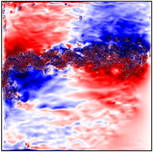
  $\phi _g$ shows more pronounced small-scale patterns in the subtropical regions. However, it also generates mesoscale components along the jet, similarly to $\varPhi _f$, thus, contradicting the assumption that the non-advective terms do not contribute as much to the mean flow and thus can be filtered out. The sign of $\varPhi _g$ is distributed differently from that of $\varPhi _f$. Their distributions are roughly perpendicular in the top layer and are the opposite in the lower two layers. Overall, the results presented highlight the necessity of interpreting the velocity potential by depth, but this is beyond the scope of this study.

Figure 5. Temporally averaged velocity potentials of divergent fluxes  $\boldsymbol {g}$ (a–c) and $\boldsymbol {f}_{div}$ (d–f) in the three layers. Units for all panels are $\times 10^2$ m $^2$ s $^{-1}$. The black solid/dashed lines represent the time-mean streamlines of the large-scale $\bar {\psi }$ with positive/negative values.
Despite the distinctions in the magnitudes and spatial patterns, negative values appear in the fields of  $K_{11,12,21,22}$ for all tensors. They are more pronounced in ${\boldsymbol{\mathsf{K}}}_{div}$, but also exist in ${\boldsymbol{\mathsf{K}}}_g$, which naturally has no relation with the rotational flux. Therefore, the removal of the rotational flux does not eliminate the negative values in the tensor components. Furthermore, the second eigenvalues of the symmetric parts of ${\boldsymbol{\mathsf{K}}}_f$ and ${\boldsymbol{\mathsf{K}}}_{div}$ are most often negative (HSSB20).
To summarise, we have presented  ${\boldsymbol{\mathsf{K}}}$, ${\boldsymbol{\mathsf{K}}}_{div}$ and ${\boldsymbol{\mathsf{K}}}_g$, and the velocity potentials $\varPhi _f$ and $\varPhi _g$. Owing to the dominance of the rotational flux $\boldsymbol {f}_{rot}$, there are major differences in the magnitudes and spatial structures of ${\boldsymbol{\mathsf{K}}}$ when compared with the other two tensors. The inclusion of $\boldsymbol {f}_{rot}$ is not responsible for the negative values or negative diffusion eigenvalues (HSSB20), as these persist for all $K$-tensors.
3.3. Non-uniqueness of diffusivity
In this section, we investigate the tracer-dependence of  $K$-tensors. We start by obtaining tracer-independent tensors for the linearly initialised tracers by exploiting the linearity of the flux-gradient relation. We then measure their relative distances to use as a reference for purely numerical discretisation errors. Next, we analyse the tracer-dependence by comparing this reference case with the relative distances of the $K$-tensors corresponding to the nonlinearly initialised tracers.
The linearity of the tracer equation and the flux-gradient relation have important consequences for the non-uniqueness of the  $K$-tensor. That is, a tensor obtained for any two tracers, $C^p$ and $C^q$, is the same as would be obtained for any other tracer that is a linear combination of $C^p$ and $C^q$. Consider two solutions $C^p$, $C^q$ of the tracer (2.6) with initial conditions $C^p(t_0)$, $C^q(t_0)$. Then, any tracer $C$ initialised as $C(t_0) = m C^p(t_0) + n C^q(t_0)$ is a solution in the form
 \begin{equation} C(t) = m C^p (t) + n C^q(t) , \end{equation}
where  $m$ and $n$ are arbitrary constants. Because the spatial filter is a linear operator, the large- and small-scale components can also be written as the above linear combination. Then, the eddy tracer flux and the large-scale tracer gradient are given by
 $$\begin{gather} \boldsymbol{f} = m \boldsymbol{f}^p + n \boldsymbol{f}^q , \end{gather}$$
 $$\begin{gather}\boldsymbol{\nabla} \bar{C} = m \boldsymbol{\nabla} \bar{C}^p + n \boldsymbol{\nabla} \bar{C}^q . \end{gather}$$
Suppose  ${\boldsymbol{\mathsf{K}}}_{f}$ is the transport tensor obtained with $C^p$ and $C^q$, then the linearity of the flux-gradient relation gives
 \begin{equation} m \boldsymbol{f}^p + n \boldsymbol{f}^q ={-} {\boldsymbol{\mathsf{K}}}_{f} \boldsymbol{\cdot} (m \boldsymbol{\nabla} \bar{C}^p + n \boldsymbol{\nabla} \bar{C}^q) , \end{equation}
and implies that  ${\boldsymbol{\mathsf{K}}}_{f}$ is also a transport tensor for $C$. Because the same linear combination as in (3.4) can be applied to the non-advective eddy terms, the associated flux divergence can be written as
 \begin{equation} \boldsymbol{\nabla} \boldsymbol{\cdot} \boldsymbol{g} = m \boldsymbol{\nabla} \boldsymbol{\cdot} \boldsymbol{g}^p + n\boldsymbol{\nabla} \boldsymbol{\cdot} \boldsymbol{g}^q . \end{equation}
Therefore, the same conclusion can be inferred for  ${\boldsymbol{\mathsf{K}}}_g$. Overall, any tracer pairs that are linear combinations of $C^p$ and $C^q$ share the same ${\boldsymbol{\mathsf{K}}}_f$ and ${\boldsymbol{\mathsf{K}}}_g$, and, thus, the same full tensor ${\boldsymbol{\mathsf{K}}}$.
It is not necessary to linearly initialise tracers to obtain the same tensor. In fact, the tracers with linear initial profiles do not always have the same tensor. Recall the initialisation of the linear profiles  $C_B$ in (2.32). Even though every linear profile has a constant gradient $(a,b)$, it can only be written as a linear combination of other pairs of linear profiles with an additional constant owing to the scalar term $\gamma$. This $\gamma$ is included in the large-scale tracer component and causes the tensors for linearly initialised tracers to be distinct. Even though it does not affect the large-scale gradient in (3.5), the eddy fluxes cannot, in general, be written as the linear combinations of those given by the linearly initialised tracers, as in (3.4), because of an additional flux component $\boldsymbol {u}'\gamma$. Thus, ${\boldsymbol{\mathsf{K}}}_{f}$ can not be unique in our linear tracer experiments, as part of the tensor component ${\boldsymbol{\mathsf{K}}}_\gamma$ depends on the scalar constant,
 \begin{equation} \boldsymbol{u}'\gamma ={-} {\boldsymbol{\mathsf{K}}}_\gamma \boldsymbol{\cdot} \boldsymbol{\nabla} \bar{C} . \end{equation}
Note that  ${\boldsymbol{\mathsf{K}}}_\gamma$ is not, in general, equal to ${\boldsymbol{\mathsf{K}}}_{rot}$, even though $\boldsymbol {u}'\gamma$ only contributes to $\boldsymbol {f}_{rot}$. Nonetheless, the transport tensor for initially linear tracers cannot be tracer-independent or unique, unless the rotational flux is removed. However, ${\boldsymbol{\mathsf{K}}}_g$ is always unique, because it only depends on $C^\prime$.
To verify this, we measure the relative distance between respective tensor components. That is, for a pair of components (denoted with superscripts  $p$ or $q$), the relative distance between them is
 \begin{equation} d_r(K^p,K^q) = \frac{1}{N_{\varOmega}}\sum_{\varOmega}\frac{|K^p - K^q |}{|\langle K \rangle|} , \end{equation}
where  $K^{p,q} \in \{K_{11}, K_{12}, K_{21}, K_{22}\}$, and the ensemble-average $\langle K \rangle$ is the global reference. For each of ${\boldsymbol{\mathsf{K}}}_f$, ${\boldsymbol{\mathsf{K}}}_{div}$ and ${\boldsymbol{\mathsf{K}}}_g$, we have 15 ensembles from RL, so in total we can measure the relative distances for 105 pairs. The standard deviation is not used as a measure owing to the large differences in magnitudes among $K$-tensors.
Figure 6 presents the relative distances for  ${\boldsymbol{\mathsf{K}}}_{f}$ and ${\boldsymbol{\mathsf{K}}}_{div}$. We see that $d_r$ for ${\boldsymbol{\mathsf{K}}}_{f}$ typically varies between 0.7 and 3, while for ${\boldsymbol{\mathsf{K}}}_{div}$ it is mainly between 0.8 and 1.25. Furthermore, more than 70 % of tensor pairs have larger distances for the former, despite the additional numerical errors induced in the latter. According to the linearity of the flux-gradient relation, ${\boldsymbol{\mathsf{K}}}_{div}$ for the linearly initialised tracers should be unique, because the tracer-dependent components ${\boldsymbol{\mathsf{K}}}_{\gamma }$ are excluded by removing the rotational fluxes. The non-zero $d_r$ for ${\boldsymbol{\mathsf{K}}}_{div}$ is attributed to numerical errors in the flux decomposition, as well as to some unavoidable alignments of gradients during the simulation. Moreover, $d_r$ can be uncommonly large for some pairs, because the ensemble-average $\langle K \rangle$ is used as a global reference in (3.9), instead of considering only $K^p$ and $K^q$. Overall, it is evident that the greater relative distances in ${\boldsymbol{\mathsf{K}}}_f$ arise from the tracer-dependent ${\boldsymbol{\mathsf{K}}}_{rot}$.

Figure 6. The relative distance  $d_r$ of components $K_{11},K_{12},K_{21},K_{22}$ (a–d) in the top layer in experiment RL. One dot represents one comparison between ${\boldsymbol{\mathsf{K}}}_{f}$ and ${\boldsymbol{\mathsf{K}}}_{div}$ given by the same tracer pairs. A total of 105 comparisons are carried out amongst the 15 tracer pairs. The $x$-values are the temporal averages of $d_r$ for ${\boldsymbol{\mathsf{K}}}_{f}$, while the $y$-values are for ${\boldsymbol{\mathsf{K}}}_{div}$.
Because  ${\boldsymbol{\mathsf{K}}}_g$ is not associated with the tracer-dependent $\gamma$, it is unique for linearly initialised tracers. This is shown in figure 7, where the relative distances for ${\boldsymbol{\mathsf{K}}}_g$ are in the range similar to those for ${\boldsymbol{\mathsf{K}}}_{div}$. As both tensors are unique, we determine the relation between them by fitting linear regression models to the comparisons for each component ( $x$ for ${\boldsymbol{\mathsf{K}}}_{div}$ and $y$ for ${\boldsymbol{\mathsf{K}}}_g$). We find that the regression lines are closely aligned with $x=y$, especially for the diagonal elements $K_{11}$ and $K_{22}$. Therefore, $d_r$ for the tensors ${\boldsymbol{\mathsf{K}}}_g$ and ${\boldsymbol{\mathsf{K}}}_{div}$ are very similar, with slight differences caused by numerical errors. This rough similarity shows that the non-uniqueness of the tensors is caused by the linearity of the flux-gradient relation and linear tracers, and may not be a property inherent to all transport tensors.

Figure 7. The relative distance  $d_r$ of components $K_{11},K_{12},K_{21},K_{22}$ (a–d) in the top layer in experiment RL. One dot represents one comparison between ${\boldsymbol{\mathsf{K}}}_{div}$ and ${\boldsymbol{\mathsf{K}}}_{g}$ given by the same tracer pairs. A total of 105 comparisons are carried out amongst the 15 tracer pairs. The $x$-values are the temporal averages of $d_r$ for ${\boldsymbol{\mathsf{K}}}_{div}$, while the $y$-values are for ${\boldsymbol{\mathsf{K}}}_{g}$. The red solid lines are the linear regression lines, and the corresponding coefficients are 1.01, 0.9, 0.79, 0.99.
To investigate if the uniqueness holds for all the passive tracers, we repeat the analyses for  ${\boldsymbol{\mathsf{K}}}_{div}$ and ${\boldsymbol{\mathsf{K}}}_g$ using the ensembles from RN. In figure 8, we scatter plot $d_r$ for the RN ensemble against $d_r$ for the RL ensemble. Most $d_r$ values for ${\boldsymbol{\mathsf{K}}}_{div}$ from RN are greater than 1.5, and all of them are larger than those from RL. The same is observed for the sum of ${\boldsymbol{\mathsf{K}}}_{div}$ and ${\boldsymbol{\mathsf{K}}}_g$. Because we have shown (analytically) that all linearly initialised tracers generate the same ${\boldsymbol{\mathsf{K}}}_{div}$ and ${\boldsymbol{\mathsf{K}}}_g$, we deduce that they are different and, thus, tracer-dependent, when the tracers are initialised with sinusoidal – or more generally, nonlinear – profiles.

Figure 8. The relative distance  $d_r$ of components $K_{11},K_{12},K_{21},K_{22}$ (a–d) in the top layer for comparisons between experiments RL and RN. The tensors are for the divergent fluxes: blue dots represent ${\boldsymbol{\mathsf{K}}}_{div}$ and orange dots represent ${\boldsymbol{\mathsf{K}}}_{div} +{\boldsymbol{\mathsf{K}}}_{g}$. The $x$- and $y$-values are the relative distances for the nonlinear and linear tracer profiles, respectively. The vertical dashed lines are located at the maximum $d_r$ for RL on $x$-axes. If a dot is to the right of its corresponding line, then $d_r$ of this tensor in RN is larger than all ensembles of $d_r$ in RL. The clouds of dots clearly show the non-uniqueness of both ${\boldsymbol{\mathsf{K}}}_{div}$ and ${\boldsymbol{\mathsf{K}}}_{div} +{\boldsymbol{\mathsf{K}}}_{g}$ for nonlinearly initialised tracers.
Until now, our conclusions are based on tracers that are relaxed towards their initial profiles. To test these conclusions for freely evolving tracers, in figure 9, we present time series of the ensemble-averaged  $d_r$ from all four experiments. For initially linear tracers, the relative differences $d_r$ increase, when the tracers are not relaxed, and this agrees with our findings regarding the numerical errors, as shown in figure 1. For nonlinear tracers, though, $d_r$ does not notably depend on the use of relaxation. Therefore, even though the relaxation effect can affect the numerical accuracy, it is irrelevant for the non-uniqueness of ${\boldsymbol{\mathsf{K}}}_{div}$. Similar observations are made for the other $K$-tensors, so we opt to not show them for brevity.

Figure 9. Evolution of  $d_r$ in the top layer for all experiments. See the legend in the upper panel for details. The panels correspond to $K_{11}$ (a), $K_{12}$ (b), $K_{21}$ (c) and $K_{22}$ (d). The difference between RL and RN, and the difference between UL and UN, are shaded in pink and purple, respectively. The relative distance increases rapidly from zero for RL and UL owing to the initial linear dependence, until the total fluxes in the domain reach equilibrium after 25 days. The black and purple lines fluctuate more, because of the higher frequency of the gradients being nearly aligned.
Because the diffusion and advection tensors have different physical interpretations, they are often separately parametrised. Therefore, it is necessary to investigate whether they are also individually tracer-dependent. To examine this, we compare the eigenvalues  $\lambda _1$, $\lambda _2$ of the diffusion tensor ${\boldsymbol{\mathsf{S}}}$ and the off-diagonal component $A_{12}$ of the advection tensor ${\boldsymbol{\mathsf{A}}}$ between the experiments RL and RN. We measure the differences by the relative ensemble standard deviation $\delta _r (\langle \cdot \rangle )$, which divides the ensemble standard deviation by the ensemble mean $\langle \cdot \rangle$. For example, $\delta _r (\langle \lambda _1 \rangle )$ is given by
 \begin{equation} \delta_r (\langle \lambda_1 \rangle ) = \frac{1}{\langle \lambda_1 \rangle} \sqrt{\frac{1}{14} \sum_{p = 1}^{15} (\lambda_1^p - \langle \lambda_1 \rangle )^2} , \end{equation}
where  $\lambda _1^p$, $p =1,\ldots , 15$, are the eigenvalues for 15 cases in one experiment.
Figure 10 shows the instantaneous fields of the relative ensemble standard deviations of the eigenvalues  $\lambda _1$, $\lambda _2$ ( $\lambda _1 \geq \lambda _2$) and of the off-diagonal element $A_{12}$. The first and second columns of panels are for RL and RN, respectively. Because the denominator of $\delta _r$ is the ensemble-mean, rather than its absolute value, the signs of the components are preserved in the figure. For both experiments, $\lambda _1$ is mostly positive in the domain and $\lambda _2$ is mostly negative. This polarity of the eigenvalues is also observed for ${\boldsymbol{\mathsf{K}}}_g$ (not shown). Therefore, we deduce that two eigenvalues are often of opposite signs in the domain even without the existence of the rotational flux, which is consistent with HSSB20. The first column shows that the ensembles of three variables for initially linear tracers do not differ much from the ensemble-means, as $\delta _r$ is predominantly less than 0.2 in the domain. This observation shows that for both ${\boldsymbol{\mathsf{S}}}$ and ${\boldsymbol{\mathsf{A}}}$, the ensembles are close to each other in distances, and agrees with our argument that ${\boldsymbol{\mathsf{K}}}_{div}$ is unique, up to numerical errors, if tracers are initially linear. For the case when tracers are initialised with nonlinear profiles, the relative ensemble standard deviations are much larger, by at least an order of magnitude. Therefore, the diffusion and the advection tensors are also tracer-dependent, that is, they are non-unique for nonlinearly initialised tracers.

Figure 10. Snapshots of the relative ensemble standard deviation  $\delta _r$ of the eigenvalues $\lambda _1$ (a,b), $\lambda _2$ (c,d) of ${\boldsymbol{\mathsf{S}}}$ and of the off-diagonal element $A_{12}$ (e,f) of ${\boldsymbol{\mathsf{A}}}$, all at day 183. Panels (a,c,e) are for RL, where tracers are linearly initialised, while (b,d,f) are for RN (nonlinearly initialised tracers). The non-uniqueness of $\lambda _1,\lambda _2$ and $A_{12}$ is observed, as the standard deviation for the latter is much larger than for the former. For both experiments, $\delta _r (\langle \lambda _1 \rangle )$ is mainly positive, as shown in (a) and (b), but $\delta _r (\langle \lambda _2 \rangle )$ is mainly negative, as shown in (c) and (d). This indicates that the eigenvalues tend to have opposite signs.
Overall,  ${\boldsymbol{\mathsf{K}}}_{div}$ and ${\boldsymbol{\mathsf{K}}}_g$ are unique for linearly initialised tracers, and any tracer dependence can serve as a measure of the numerical errors in our approach. The comparison with more general, nonlinearly initialised tracers demonstrates the inherent dependence of the $K$-tensor on the tracer pairs, and, thus, its non-uniqueness. This conclusion is not affected by a relaxation forcing. The same argument also applies to the eigenvalues of the diffusion tensor and to the off-diagonal element of the advection tensor. It is worth noting that the non-uniqueness of $K$-tensors is not limited to the idealised QG model but is also found in a more comprehensive general circulation model (GCM) of the entire Atlantic Ocean (Kamenkovich et al. Reference Kamenkovich, Berloff, Haigh, Sun and Lu2021).
4. Conclusions and discussion
This work aimed to investigate the uniqueness of the transport  $K$-tensor in an eddy-resolving model, with the long-term motivation of parametrising eddy tracer fluxes in coarse-resolution ocean models. Our objective here was to calculate $K$-tensors from high-resolution flow and tracer distributions, to investigate the resulting errors in the eddy flux reconstructions and to examine the $K$-tensors’ dependencies on the passive tracers. The main conclusion is that the $K$-tensors depend on the tracer and are, therefore, non-unique. This non-uniqueness is strongly influenced by the rotational (non-divergent) component of the eddy tracer flux.
A double-gyre, mid-latitude QG model was used in the study. Tracers were initialised with either linear or nonlinear (sinusoidal wave) profiles, and were advected by the flow for half a year. The flow and tracer fields were decomposed into large- and small-scale components using a spatial filtering method. The resulting eddy forcing  $E$ consisted of the divergence of the eddy tracer flux $\boldsymbol {f}$ and non-advective eddy terms. We assumed a flux-gradient relation to link $\boldsymbol {f}$ to the large-scale tracer gradient $\boldsymbol {\nabla } \bar {C}$ via a transport tensor ${\boldsymbol{\mathsf{K}}}_f$. By quantifying the non-advective eddy terms using a divergent flux $\boldsymbol {g}$, we obtained the corresponding $K$-tensor ${\boldsymbol{\mathsf{K}}}_g$. Then, the full tensor ${\boldsymbol{\mathsf{K}}}$ corresponding to the eddy forcing was given by the sum of ${\boldsymbol{\mathsf{K}}}_f$ and ${\boldsymbol{\mathsf{K}}}_g$. The divergent tensor ${\boldsymbol{\mathsf{K}}}_{div}$ – that is, the portion of ${\boldsymbol{\mathsf{K}}}_f$ corresponding to the divergent eddy flux $\boldsymbol {f}_{div}$ – was obtained by applying the Helmholtz decomposition to $\boldsymbol {f}$. The non-advective eddy forcing terms were comparable in size to $\boldsymbol {\nabla } \boldsymbol {\cdot } \boldsymbol {f}=\boldsymbol {\nabla } \boldsymbol {\cdot } \boldsymbol {f}_{div}$, and similarly the $K$-tensor ${\boldsymbol{\mathsf{K}}}_g$ was as large as ${\boldsymbol{\mathsf{K}}}_{div}$. Therefore, we deduce that the non-advective terms should be parametrised along with the advective eddy terms.
The accuracy of the inversion method for computing the  $K$-tensors was measured by reconstructing $\boldsymbol {f}$, $\boldsymbol {\nabla } \boldsymbol {\cdot } \boldsymbol {f}$ and $E$. Generally, ${\boldsymbol{\mathsf{K}}}$ is two orders of magnitude larger than ${\boldsymbol{\mathsf{K}}}_{div}$, owing to the dominant rotational fluxes (Marshall & Shutts Reference Marshall and Shutts1981). Despite this difference, both tensors were shown to be capable of reconstructing the eddy tracer flux convergence, with their parametrised flux convergences being visually indistinguishable from each other. The largest errors were typically found in the eastward jet region where the eddies were most energetic, but for initially nonlinear tracers, they also occurred in regions where the tracer profiles exhibited sharp spatial gradients (a consequence of the randomly selected nonlinear profiles).
Large errors in the reconstructed flux divergence are introduced by the Helmholtz decomposition, more precisely by the divergence operator, and hence errors associated with  ${\boldsymbol{\mathsf{K}}}_{div}$ are much larger than those for ${\boldsymbol{\mathsf{K}}}$. This is despite the fact that the corresponding flux convergences are visually indistinguishable from each other. As the transport tensor component associated with the rotational flux is eliminated automatically under the divergence operator in the tracer evolution equation, it seems more suitable to use ${\boldsymbol{\mathsf{K}}}_f$ rather than ${\boldsymbol{\mathsf{K}}}_{div}$ for a parametrisation, given the errors associated with the latter. However, the additional model errors induced by simplifications in parametrisations may be as large as the errors induced by the flux decomposition. Therefore, the question of whether the difference in errors remains significant after smoothing the fields for coarse-grid models needs to be answered.
For each  $K$-tensor, the tracer-dependence was quantified by measuring the relative distances among its ensembles given by different tracer pairs. We analysed how the tracer-dependence of the $K$-tensors was affected by various factors such as the initial tracer profiles, the rotational flux and the relaxation forcing. We found that ${\boldsymbol{\mathsf{K}}}_{div}$ and ${\boldsymbol{\mathsf{K}}}_g$ were unique, up to numerical errors, if the tracers were initialised with linear profiles, owing to the linearity of the flux-gradient relation. However, ${\boldsymbol{\mathsf{K}}}_f$ and, thus, the full tensor ${\boldsymbol{\mathsf{K}}}$ were found to be tracer-dependent because the dominant rotational component (i.e. that corresponding to the rotational flux) was tracer-dependent. For nonlinearly initialised tracer profiles, the uniqueness of ${\boldsymbol{\mathsf{K}}}_{div}$ and ${\boldsymbol{\mathsf{K}}}_g$ was lost, and the non-uniqueness of ${\boldsymbol{\mathsf{K}}}$ was further amplified by the presence of the tracer-dependent rotational flux. Therefore, in general, $K$-tensors are non-unique for passive tracers. The conclusion can be extended to diffusion tensor ${\boldsymbol{\mathsf{S}}}$ and advection tensor ${\boldsymbol{\mathsf{A}}}$, separately. Finally, switching off the relaxation forcing did not affect the non-uniqueness for nonlinear tracers.
The effect of the non-uniqueness of the eddy transport tensor on parametrisations needs to be investigated. Generally, the estimation of the eddy flux for a tracer is different when using different tensors. A question then arises: does it make a fundamental difference whether one uses the tensor given by a tracer pair including this tracer or any tensor from any tracer pair? If not, can these tensors be implemented for the stochastic estimations of the eddy flux patterns? Stochastic closures have been employed in the past (Berloff & McWilliams Reference Berloff and McWilliams2003; Grooms Reference Grooms2016), and our study suggests that treating the eddy transport tensor as a random process may be consistent with its inherent non-uniqueness. In situations when the large-scale flow varies much slower than the eddies, a deterministic solution can be obtained as the tensor given by the flux-gradient relation between  $\overline {\boldsymbol {u}^\prime C^\prime }$ and the steady large-scale gradient $\bar {C}$, where $\bar {\cdot }$ denotes the Reynolds averaging. Whether the difference between such tensors and our non-unique transport tensor (which is supposed to be given by the variations of the large-scale terms in the eddy flux) can be treated as stochastic variations still needs to be investigated.
Acknowledgements
We are grateful to Dr S. Bachman and the anonymous reviewers for their valuable and helpful comments.
Funding
P.B. gratefully acknowledges funding by the NERC, UK grants NE/R011567/1 and NE/T002220/1, and by the Moscow Center for Fundamental and Applied Mathematics (supported by the Agreement 075-15-2019-1624 with the Ministry of Education and Science of the Russian Federation). I.S. and P.B. were also supported by the Leverhulme Trust grant RPG-2019-024. M.H. is gratefully supported by the ‘Imperial CoA NERC’ covid-extension grant. Igor Kamenkovich acknowledges support by the NSF, grant 1849990.
Declaration of interests
The authors report no conflict of interest.


 Open access