


1. Introduction
The propagation of a lock-release gravity current (GC) over a downslope is a topic of active investigation (Maxworthy Reference Maxworthy2010; Dai Reference Dai2013; van Reeuwijk, Holzner & Caulfield Reference van Reeuwijk, Holzner and Caulfield2019; Zemach et al. Reference Zemach, Ungarish, Martin and Negretti2019; Gadal et al. Reference Gadal, Mercier, Rastello and Lacaze2023; Han et al. Reference Han, He, Lin, Wang, Guo and Yuan2023). The counterpart propagation over a horizontal surface has been successfully covered by the classical shallow-water (SW) model (with no entrainment and zero drag) which predicts analytically the important stages of slumping ( $x_N \propto t$, i.e. a constant speed of propagation $u_N$) and large-time self-similar behaviour (with $x_N \propto t^{2/3}$), as summarized by Ungarish (Reference Ungarish2020); here $x_N$ is the position of the nose, and $t$ the time. The use of the SW formulation for the inclined GC is more problematic because (a) there is an additional (slope-driving) term in the momentum equation, and (b) the modelling of a realistic flow in this case must take into account entrainment and drag from an early stage (see Zemach et al. Reference Zemach, Ungarish, Martin and Negretti2019). These additional effects have defied reliable analytical solutions of the SW equations.
An analytical propagation formula of the inclined GC was derived by Beghin, Hopfinger & Britter (Reference Beghin, Hopfinger and Britter1981). This approximation, called thermal theory, postulates that the GC is a self-similar box of oval shape. Entrainment and drag are taken into account as global contributions to the box balances, but a front-jump condition (which is an essential component in the flow of the inertia–buoyancy GC, see Benjamin (Reference Benjamin1968)) is not, and cannot be, imposed. The solution predicts a  $t^{2/3}$ propagation for large time, but the quantitative result depends on adjustable constants that must be calibrated for each individual system. In any case, the $x_N \propto t^{2/3}$ trend has been confirmed by reliable experiments (e.g. Maxworthy Reference Maxworthy2010; Dai Reference Dai2013), and seems to describe a physical pattern of the GC on a slope. This raises the question if the more reliable SW formulation also predicts this type of behaviour in analytical form.
Here we attempt to close this gap of knowledge by developing and testing a self-similar solution for the large-time GC inclined flow with drag and entrainment. The conclusion is that, under some plausible simplifying assumptions, a closed solution exists that displays physically acceptable profiles for the flow-field variables and  $x_N \propto t^{2/3}$ propagation.
The structure of the paper is as follows. The formulation of the SW equations and boundary conditions is presented in § 2. The self-similarity solution is developed in § 3. In § 4 we show some test-case comparisons with experimental data, and discuss the insights of the results and the need for future work for a sharper assessment of the predictions.
2. Formulation
We use dimensional variables unless stated otherwise. The variables of the ambient fluid are denoted by the subscript  $a$, while those of the current are without subscript (or with subscript $c$ when emphasis is needed).
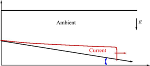
The system is sketched in figure 1. We use a Cartesian  $xz$ two-dimensional (2-D) system with $x$ horizontal and $z$ vertically upward, and corresponding $u,w$ velocity components. Gravity $g$ acts in the $-z$ direction. For simplicity, and in accord with typical laboratory systems, the slope $\gamma$ of the bottom is constant. The lock is defined by the backwall $x=0$, dam (gate) at $x=x_0$ and is of height $h_0$ above the bottom. The height of the ambient is $H(x)$, assumed large as compared with $h_0$. Consequently (a) the return flow $u_a = - u h /H$ in the ambient is negligible, which justifies the use a one-layer SW model, and (b) the details of the top (open surface or solid lid) are unimportant. (We consider the propagation in the horizontal $x$ direction. The switch to the slope-aligned ground coordinate (subscript $S$ is $(x_S, u_S)=(x, u)/\cos \gamma$ and the corresponding perpendicular height of the GC is $h_S = h(x,t) \cos \gamma$. The change is typically small because we assume that $\gamma$ is small ( $\tan \gamma \lesssim 0.2$, say) otherwise $D w/ D t$ violates the hydrostatic approximation used in the SW model.) In these cases $1-\cos \gamma < 2\,\%$. The experimental data of Maxworthy (Reference Maxworthy2010), Dai (Reference Dai2013), Gadal et al. (Reference Gadal, Mercier, Rastello and Lacaze2023) and Han et al. (Reference Han, He, Lin, Wang, Guo and Yuan2023) satisfy this restriction.

Figure 1. Sketch of the system. The GC is initially ( $t=0$) in the lock (dashed line) of dimensions $x_0, h_0$. Here $x_S = x/\cos \gamma$ is the along-slope coordinate. (The top is usually a free surface; in the present analysis this detail is unimportant.)
The ambient fluid is of constant density  $\rho _{a}$. The current is, initially, of homogeneous density $\rho _{c}(t=0) >\rho _{a}$. Due to entrainment this is diluted to $\rho _{c}(x,t)$. The dilution is expressed by the concentration function
 \begin{equation} \phi(x,t) = \frac{\rho_{c}(x,t) - \rho_{a}}{\rho_{c}(t=0) - \rho_{a}}, \end{equation}
with the initial condition  $\phi = 1$ in the lock. After release, $\phi (x,t) \le 1$. The initial reduced gravity is $g' = [ \rho _{c}(t=0)/ \rho _{a} - 1 ] g$ and the effective reduced gravity is $g'_e = \phi g'$, where $g$ is the gravity acceleration.
We consider a Boussinesq inertial–buoyancy (large-Reynolds-number) GC, affected by entrainment (of rate  $E |u|$) and drag (of form $c_D \rho _{c} u|u|$) where $E$ and $c_D$ are dimensionless coefficients, typically small.
The equations for the volume of the current, mass of the dense component (represented by  $g'_e$) and momentum of the current (see Ungarish (Reference Ungarish2020), § 11.2) in dimensional form are
 $$\begin{gather} \frac{\partial h}{\partial t} + \frac{\partial}{\partial x} (uh) = E |u|, \end{gather}$$
 $$\begin{gather}\frac{\partial g_e' h}{\partial t} + \frac{\partial}{\partial x} (g'_e uh) = 0, \end{gather}$$
 $$\begin{gather}\frac{\partial}{\partial t} (uh) + \frac{\partial}{\partial x} \left(u^2 h+ \frac{1}{2} g'_e h^2\right) = g'_e h \tan \gamma -c_D u |u|. \end{gather}$$
The calculation of  $g'_e(x,t)$ is a part of the problem. The condition at the nose $x=x_N(t)$ is
 \begin{equation} u_N = \dot{x}_N = Fr [(g'_e )_N h_N]^{1/2} = Fr [g' \phi_N h_N]^{1/2}, \end{equation}
where the upperdot denotes time derivative and the subscript  $N$ denotes the nose (front) position. Here $Fr$ is the nose-jump Froude number, whose value is expected to be close to $\sqrt {2}$. (Actually, slightly smaller. This is justified by a control-volume analysis, e.g. Ungarish (Reference Ungarish2020), § 4.3, for an inclined channel. In a deep ambient, the thin jump is dominated by the instantaneous driving force $g'_e h_N$ and dynamic reaction $(u_N/ \cos \gamma )^2 /2$. The details are cumbersome and outside the scope of this paper.)
To facilitate the analysis, hereafter we switch to dimensionless variables:  $x$ is scaled with $x_0$, $h$ with $h_0$, velocity with $U_{ref} = (g' h_0)^{1/2}$ and time with $T_{ref} = x_0/U_{ref}$. Next, we introduce the stretched horizontal coordinate
 \begin{equation} \xi = x/x_N(t) \quad (0 \le \xi \le 1) \end{equation}
and transform the flow-field variables to dependency on  $\xi,t$ (instead of $x,t$) (see Ungarish Reference Ungarish2020). The transformed system of equations, in dimensionless form reads
 \begin{align} & \left[\begin{array}{c} h\\ \phi \\ u \end{array}\right]_t +\frac{1}{x_N} \left[\begin{array}{lll} u - \dot{x}_N \xi & 0 & h \\ 0 & u -\dot{x}_N \xi & 0 \\ \phi & \dfrac{1}{2} h & u -\dot{x}_N \xi \end{array}\right] \left[\begin{array}{c} h \\ \phi \\ u \end{array}\right]_\xi \nonumber\\ &\quad = \lambda \left[\begin{array}{c} E |u| \\ -\phi E \dfrac{|u|}{h} \\ \phi \tan \gamma - (c_D + E )\dfrac{u|u| }{h} \end{array}\right], \end{align}
where  $\lambda = x_0/h_0$ is the lock aspect ratio of the order of unity. The system is subject to
 \begin{equation} \dot{x}_N = Fr (\phi_N h_N)^{1/2} \quad \text{and}\quad x_N \int_0^1 \phi(\xi,t) h(\xi,t)\,{\rm d} \xi = 1. \end{equation}
The first equation of (2.8a,b) is the nose-jump condition and the second equation expresses the global conservation of the dense component (and hence of the initial buoyancy). The position of the nose is  $\xi = 1$. We keep in mind that $E$ and $c_D$ are small (of the order of 0.01), $\gamma \lesssim 0.2$, $Fr \approx \sqrt {2}$, and $\lambda$ is of the order of unity. These values are not relevant for the derivation of the mathematical solution, but are important for the interpretation of the results.
3. Similarity solution
For progress we assume that  $Fr, E, c_D$ and $\gamma$ are constants. For brevity of notation, we shall use $\gamma$ instead of $\tan \gamma$ (this can be corrected in the final results if needed).
We seek a similarity solution of the form  $x_N = K t^\beta$ while the $h,\phi,u$ fields vary as $t^a, t^b, t^c$, where $K,\beta,a,b,c$ are constants (see also Ross, Dalziel & Linden (Reference Ross, Dalziel and Linden2006), appendix B). After some algebra we find that the only non-trivial solution requires $\beta = 2/3, a = 2/3, b = -4/3, c = -1/3$. It is convenient to express this dependency as follows:
 \begin{align} x_N = Kt^{2/3},\quad \dot{x}_N = \tfrac{2}{3} K t^{{-}1/3},\quad h = \mathcal{H}(\xi) \cdot \dot{x}_N^{{-}2},\quad \phi = \mathcal{P} (\xi) \cdot \dot{x}_N^4,\quad u = \mathcal{U}(\xi) \cdot \dot{x}_N, \end{align}
with the boundary condition  $\mathcal {U}(0) = 0,\ \mathcal {U}(1) = 1$. The task is to calculate the profile functions $\mathcal {H}, \mathcal {P}, \mathcal {U}$ and the value of $K$. To this end, we substitute these relationships into the governing equations (2.7). We obtain, after some algebra, the reduced equations of volume continuity, dense mass continuity and momentum, as follows:
 $$\begin{gather} \mathcal{H} + (\mathcal{U} - \xi) \mathcal{H}' + \mathcal{H} \mathcal{U}' = \lambda \varOmega E \mathcal{U}, \end{gather}$$
 $$\begin{gather}- 2 \mathcal{P} + (\mathcal{U} - \xi) \mathcal{P}' ={-} \lambda \varOmega E \mathcal{P} \mathcal{U}/ \mathcal{H}, \end{gather}$$
 $$\begin{gather}- \frac{1}{2} \mathcal{U} + (\mathcal{U} - \xi) \mathcal{U} ' + \mathcal{H} ' \mathcal{P} + \frac{1}{2} \mathcal{H} \mathcal{P} ' = \lambda \varOmega E \left[\mathcal{P} \frac{\gamma}{E} -\left(\frac{c_D}{E}+1\right) \frac{\mathcal{U}^2}{\mathcal{H}}\right], \end{gather}$$
where the prime denotes  $\xi$ derivative, and
 \begin{equation} \varOmega = (2/3)^2K^3. \end{equation}
Equations (2.8a,b) yield
 $$\begin{gather} Fr^2 \mathcal{P}(1) \mathcal{H}(1) =1, \end{gather}$$
 $$\begin{gather}\varOmega \int_0^1 \mathcal{P}(\xi) \mathcal{H}(\xi)\,{\rm d} \xi = 1. \end{gather}$$
For the verification of the reduction note the relations:  $x_N \dot {x}_N^2 = \varOmega$ and $\ddot {x}_N = -(1/2) \dot {x}_N^4/\varOmega$.
By inspection we find that the volume and mass continuity equations (3.2) and (3.3) are solved by
 \begin{equation} \mathcal{U} = \xi,\quad \mathcal{H} = \tfrac{1}{2} \lambda \varOmega E \xi, \end{equation}
and this solution reduces (3.4) to
 \begin{equation} \hat{\mathcal{P}}' \xi + \sigma \hat{\mathcal{P}} ={-} (6 + 8 c_D/E)\xi, \end{equation}
where
 \begin{equation} \mathcal{P} = \frac{1}{\lambda \varOmega E}\hat{\mathcal{P}}(\xi),\quad \sigma = 2 - 4 \gamma/E. \end{equation}
Assume  $\sigma < 0$, i.e. $\gamma > E/2$, which is a plausible and mild restriction. This restriction is necessary because for $\gamma \le E/2$ the solution $\hat {\mathcal {P}}$ diverges at $\xi = 0$. The solution of (3.8), subject to the boundary condition (3.6a) (i.e. $\hat {\mathcal {P}}(1) = 2/Fr^2$), is as follows:
(a) for  $\sigma \ne -1$ (i.e, $\gamma \ne\ (3/4) E$)
 \begin{equation} \hat{\mathcal{P}} ={-} \frac{6+ 8 c_D/E }{1 + \sigma} ( \xi - \xi ^{- \sigma}) + \frac{2}{Fr^2} \xi^{- \sigma}, \end{equation}
 (b) for  $\sigma = -1$ (i.e, $\gamma = (3/4) E$)
 \begin{equation} \hat{\mathcal{P}} ={-}(6+ 8 c_D/E) \xi \ln \xi + \frac{2}{Fr^2} \xi. \end{equation}
We note that (3.10) is a good approximation to (3.9) in the interval  $\pm 0.02$ about $\sigma = -1$ which means that $\max \hat {\mathcal {P}}$ is bounded by $(3 + 4 c_D/E)$, roughly, in spite of the large leading coefficient in (3.9) near $\sigma = -1$. In other words, $\sigma = -1$ is not a problematic point in this solution.
The boundary conditions  $\mathcal {U}(0) =0,\ \mathcal {U}(1) = 1$ and (3.6a) are satisfied, and $\hat{\mathcal{P}}$ is positive for $\xi \in (0,1]$. To close the solution we must calculate the constants $\varOmega$ and $K$. The values are provided by (3.6b) and (3.5). After some algebra we obtain, for $\gamma > E/2$,
 $$\begin{gather} \varOmega =4 \frac{\gamma}{E} \left(1 + \frac{1}{Fr^2} + \frac{4} {3}\frac{c_D}{E}\right)^{{-}1}, \end{gather}$$
 $$\begin{gather}K =\left ( \frac{9}{4} \varOmega \right )^{1/3} = \left (9 \frac{ \gamma}{E} \right ) ^{1/3} \left (1 + \frac{1}{Fr^2} + \frac{4} {3}\frac{c_D}{E} \right )^{{-}1/3}. \end{gather}$$
We recall that  $\gamma$ stands for $\tan \gamma$. Since $K$ and $\varOmega$ are positive, the results (3.7a,b) and (3.9)–(3.10) for the profiles $\mathcal {U}, \mathcal {H}$ and $\mathcal {P}$ are physically acceptable. The solution satisfies the equations of motion, boundary conditions at $\xi = 0$ and $1$, and conservation of the dense component.
Finally, the solution must satisfy the condition  $\phi \le 1$ which reads
 \begin{equation} \max \phi = (\lambda \varOmega E)^{{-}1} \max [ \hat{\mathcal{P}}(\xi)] \cdot \dot{x}_N^4 =\left(\frac{2}{3}\right)^2 \frac{K}{\lambda E} \max [ \hat{\mathcal{P}}(\xi) ] \cdot t^{{-}4/3} \le 1. \end{equation}
The leading coefficient  $K/E$ behaves like $(\gamma /E^4)^{1/3}$, which is typically a large number. Therefore, the condition (3.13) provides an estimate for the time $t_{min}$ (of the order of $\gamma ^{1/4} E^{-1} \gg 1$) after which the similarity solution is physically acceptable. As expected, this is a long-time behaviour. The volume of the GC is
 \begin{equation} V = V(t) = x_N \dot{x}_N^{{-}2} \int_0^1 \mathcal{H}(\xi)\,{\rm d} \xi = \frac{1}{4} \lambda E K^2 t^{4/3}. \end{equation}
We expect  $V(t)>1$. This is fulfilled when $\phi <1$ (i.e. $t>t_{min}$) because the volume-integral of the diluted dense fluid is conserved (equals 1) according to the imposed condition (b) of (2.8a,b). The entrainment which causes the decay of $\phi$ increases the volume of the GC.
4. Discussion
The similarity solution derived here is meaningful for propagation downslope,  $\gamma > E/2 >0$. The solution is clearly non-physical for $\gamma \le E/2$. This explains why the analysis of Johnson & Hogg (Reference Johnson and Hogg2013) for a horizontal ( $\gamma = 0$) GC with entrainment and drag did not indicate this type of long-time pattern.
The profiles  $\mathcal {U}$ and $\mathcal {H}$ are simple lines. Typical profiles of $\hat{\mathcal{P}}(\xi )$, which represent the concentration of the dense component, are shown in figure 2. The prediction is that $\hat{\mathcal{P}}(\xi )$ depends on $Fr^2, \gamma /E$ and $c_D/E$. In the figure, all lines are for $Fr^2 = 2$, and various pairs of $\gamma /E, c_D/E$ as shown on the lines. All the profiles (for $\gamma > E/2$) vary from 0 to 1 at the edges of the GC, but in some cases with large $c_D/E$ a pronounced maximum is attained. The dilution is a complex process, dominated by entrainment and convection, and constrained by the conservation of the dense component. This explains why $\hat{\mathcal{P}}$ is a non-linear function of the input parameters. Since $\mathcal {H} = c \xi$ it is evident that, typically, the mass of the dense component is concentrated in the frontal part of the GC, $\xi >0.6$, say.

Figure 2.  $\hat {\mathcal {P}}$ vs $\xi$ for ( $\gamma /E, c_D/E)$ pairs shown on the lines. Here $Fr^2 = 2$.
We think that the major importance of the results is the propagation behaviour  ${x_N = K t^{2/3}}$. First, we emphasize that this is a rigorous (exact solution) prediction of the SW equations. Second, we give a simple and insightful analytical result for the dimensionless coefficient $K$. The driving effect is $\gamma ^{1/3}$. When the drag is not large ( $c_D/E <10$, say), the slope driving is balanced by entrainment, $K \propto (\gamma /E)^{1/3}$. When the drag is more significant than entrainment, $K \propto (\gamma /c_D) ^{1/3}$. The dimensionless propagation coefficient $K$ is of the order of unity for typical cases ( $\gamma \sim 0.1,\ E \sim 0.01,\ c_D/E \sim 1$). For dimensional $x^\ast _N$ and time $t^\ast$ the similarity propagation is
 \begin{equation} x^\ast_N = K (g' x_0 h_0)^{1/3} (t^\ast)^{2/3}. \end{equation}
As expected, at large times only the buoyancy  $g' x_0 h_0$ of the initial lock determines the coefficient of the $t^{2/3}$ propagation, for any aspect ratio $\lambda$. The result (4.1) is formally the same as for the classical horizontal GC, but (a) the coefficient $K$ is of course different ( $[27 Fr^2/(6 - Fr^2)]^{1/3}$, see Ungarish (Reference Ungarish2020) § 3.4.1), and (b) the classical similarity appears soon after the slumping stage (during which the nose velocity $u_N$ is constant).
Another interesting result is the angle  $\alpha$ of the triangle profile of the current. We note that in dimensional form (3.7a,b) yields
 \begin{equation} h^{\ast} = \tfrac{1}{2} E x^\ast,\quad (0 \le x^\ast \le x_N^\ast). \end{equation}
Surprisingly,  $\alpha$ is independent of $\gamma, c_D$ and $Fr$.
$Fr$.
The self-similar solutions of the classical lock-release GCs display a virtual-origin difficulty, which also shows up in the present solution. Indeed, our solution does not satisfy initial conditions at  $t=0$, and the solution remains valid when we shift $t$ by an arbitrary time-shift constant, $\tau$, to $t+\tau$. This gives rise to the question which initial conditions will produce convergence of the solution of the SW system to the similarity solution. There is no formal answer (to our knowledge) but various tests indicate that numerical (finite-difference) solutions for lock-release from rest in simple-shaped reservoirs approach the self-similar behaviour for large $t$ (see Ungarish Reference Ungarish2020). This is supported by experimental evidence that the long-time propagation of GCs is in accord with the similarity-solution predictions, for various systems; this is also valid for the present configuration, as shown below. Consequently, in spite of the mathematical rigour, this solution is not a self-contained quantitative prediction tool. On the other hand, this undetermined time-shift constant $\tau$ can be used to match $x_N(t_m)$ of a realistic GC to the self-similar $K (t_m + \tau )^{1/3}$, under the expectation that this is a good approximation for $t>t_m$. Since a realistic GC at a given $t$ after release is bound to be influenced (to some degree) by the initial conditions, the value of $\tau$ is expected to depend on the aspect ratio of the lock $\lambda$ and on the initial depth of the lock.
The mathematical rigour does not guarantee physical accuracy. The assumption of constant  $E$ and $c_D$ for the entire process lacks physical justification, but we argue that the use of some proper representative values is expected to produce a good approximation to the more complex behaviour. The verification requires accurate experimental or Navier–Stokes simulation data, which is presently unavailable.
Published experimental studies for lock-release GCs over a slope (e.g. Maxworthy Reference Maxworthy2010; Dai Reference Dai2013) have reported the tendency for  $t^{2/3}$ propagation at long times after release (typically $t>20$, dimensionless). These qualitative agreements are an encouraging support to the SW similarity solution. However, it is not possible to make a sharp comparison of our results with the data, because there are too many uncertainties, in particular, the adjustable time-shift $\tau$ of the virtual time origin, and the values of $c_D$ and $E$. Moreover, the available data cover only a limited distance of propagation in the validity domain of our solution (because experiments with long slopes require deep and expensive tanks). We illustrate this with the following test case.
We consider the experiments of Dai (Reference Dai2013) for propagation on slopes of Boussinesq GCs with the following properties:  $x_0 = 10\,\mathrm {cm},\ h_0 = 8\,\mathrm {cm}$, $g'= 17.11\,\mathrm {cm}\,{\rm s}^{-2}$. The data used here, shown by the symbols in figure 3, were taken by digitization and scaling of the figures 4(a) and 9(b) of Dai (Reference Dai2013). For the SW predictions (green lines) we use the theoretical $Fr = \sqrt {2}$ and the experimentally based tentative estimates $E = 0.015$ and $c_D/E = 7$ (Negretti, Flor & Hopfinger Reference Negretti, Flor and Hopfinger2017; Gadal et al. Reference Gadal, Mercier, Rastello and Lacaze2023).

Figure 3. The  $x_N$ vs $t$ experiment (symbols) and prediction (line) for (a) $\gamma = 9^\circ$ and (b) $\gamma = 6^\circ$. The matching point is marked by $X$. Here $c_D/E = 7$ for green lines, $c_D/E = 5$ for the dash-dot black line in (b).
First, we consider the slope  $\gamma = 9^\circ$. This yields $K = 2.06$, see (3.12). We fit the prediction $x_N(t) = K (t +\tau )^{2/3}$ to the measured point $x_m = 14.0$ at $t_m=20.53$, and we obtain $\tau = -2.84$. We see in figure 3(a) a remarkably good agreement between data and theory for this case for $10 < t <36$ (end of available data). Surprisingly, the agreement starts well before the matching point. This is most likely just a coincidence, because at $t= 10$ the experimental GC is barely at the end of the slumping stage (the transition from the initial stagnant rectangle into a long moving current), and we do not expect this type of agreement in general. Next, we consider the slope $\gamma = 6^\circ$. We obtain $K = 1.80$, and matching at $x_m = 17.47,\ t_m = 27.1$ yields $\tau = 2.45$ We see in figure 3(b) a fair-to-good agreement. However, the discrepancy is larger than for the $\gamma = 9^\circ$ case. Since the green line is systematically below the symbols as $t$ increases, we infer that a smaller $c_D$ may improve the result. We change to $c_D/E=5$, obtain the new $K=1.98$ and $\tau = -1.53$. The corresponding prediction, displayed as the black dash-dot line in figure 3(b), is in good agreement with the data. Figure 4 shows the log–log plots of the propagations of the previous figure, and also the $2/3$-slope line. The slight deviation from the ideal slope is due to the virtual-origin shift $\tau$.

Figure 4. The  $x_N$ vs $t$ experiment (symbols) and prediction (line) log–log plot. Details as in caption of figure 3.
The long-time  $t^{2/3}$ propagation has also been detected by the experiments of Maxworthy (Reference Maxworthy2010), but the data have been reported in an implicit form that precludes a detailed comparison. Moreover, the experiments of Dai (Reference Dai2014) demonstrate that the $t^{2/3}$ pattern applies also to non-Boussinesq systems.
These comparisons are encouraging, but not sharp. The values of  $E$ and $c_D/E$ are uncertain (these coefficients are expected to depend on a local Richardson number, and perhaps also on a Reynolds number, but the details are still under investigation, e.g. van Reeuwijk et al. (Reference van Reeuwijk, Holzner and Caulfield2019)). We note in passing that the bulk Richardson number, $g'_e h/u^2$ (dimensional variables), is a function of $\xi$ only, which may facilitate the choice of the averaged constant $E$ and $c_D$ when more information becomes available. The choice of the matching point (time $t_m$ or distance $x_m$) is debatable. The experimental data cover a non-large length of propagation, and some disagreements at larger propagation cannot be ruled out. Special care may be needed to separate the drag and entrainment contributions from the hindering effect of the viscous terms (discarded in the SW equations) which is also enhanced with propagation. Johnson & Hogg (Reference Johnson and Hogg2013) emphasize that the effects of turbulent entrainment (essential in the present solution) occur at long times, which are of relevance in large-scale flows in nature and environment, but cannot be well reproduced in typical laboratory experiments before the flow becomes contaminated by viscous effects. The conclusion is that the present theory can be used for tentative predictions, but conclusive tests must wait for future work. In any case, the long-time similarity solution is expected to point out a tendency to an asymptotic behaviour also for small-scale GCs. There may be some hybrid cases in which the similarity solution and the viscous effects coexist, resulting in a $t^{2/3}$ propagation although the other details of the similarity solution (such as the triangular height profile) are obscured by viscous smoothing.
The present similarity solution indicates a non-physical behaviour of  $\mathcal {P}(\xi )$ for $\gamma < E/2$. The reason is unclear. The experiments of Dai (Reference Dai2013) show a change of long-time behaviour for $\gamma = 2^\circ$ (as compared with the $6^\circ$ and $9^\circ$ cases) which may be a manifest of the failure of the present similarity balances for small slopes. We keep in mind that for $\gamma =0$ the SW equations admit a $x_N \propto t^{2/3}$ similarity based on different balances (zero entrainment and drag). The gap $0<\gamma \lesssim 2^\circ$ between these different balances may defy a similarity approach.
The  $x_N \propto t^{2/3}$ long-time propagation is also predicted by the ‘thermal theory’ (Beghin et al. Reference Beghin, Hopfinger and Britter1981). This approximation models the dense fluid as a box of oval shape, and does not use the front-jump condition. It is therefore interesting that, nevertheless, there are some agreements between this solution and the SW rigorous result, in particular, the propagation is with $t^{2/3}$ and admits a virtual-origin time-shift, and the coefficient of $t^{2/3}$ is ${\propto }$ $\gamma ^{1/3}$. However, the thermal theory $x_N(t)$ formula contains some postulated shape-factors and $x$-virtual-origin adjustable parameters that preclude a conclusive comparison. We argue that the SW similarity solution is a more reliable prediction. First, it has been derived from a clear-cut set of governing equation; the only additional restrictions are that $E$ and $c_D$ are constants, which are clear-cut physical assumptions. Second, the profiles of $h$,
$h$,  $u$ and $\phi$ have been calculated, not postulated. Third, the self-similar solution is a generic tool in the theory of GCs, which works well for many different systems (with and without stratification, in Cartesian and cylindrical geometries), while the thermal theory is an ad hoc patch. We hope that future work will provide more information about the merits and deficiencies of the SW exact solution, and also theoretical or empirical improvements. A formally straightforward assessment of the analytical solution can be achieved by the numerical integration of the SW equations with plausible initial conditions. This is a non-trivial task because small parameters ( $E,c_D,\gamma$) and long times are involved, and hence special high-accuracy codes (e.g. Skevington & Hogg Reference Skevington and Hogg2024) must be employed. We hope that this paper will motivate such studies.
Acknowledgements
The author thanks an anonymous referee for clarifications concerning the range of applicability of the solution  $\hat{\mathcal{P}}(\xi )$.
Declaration of interests
The author reports no conflict of interest.


 Open access