


1. Introduction
Porous obstructions in water flows can be arranged in various configurations. For example, transplanted mangrove shoots in restoration programmes are normally arranged into parallel inline rows (figure 1a); jacket structures are designed as a three-dimensional (3-D) truss with elements often having different orientation depending on the local load they withstand (figure 1b); foundation piles can be organised in a concentric ring (figure 1c); and tidal turbines are often arranged in staggered or inline patterns (figure 1d). The arrangement of these systems is often driven by hydrodynamic factors. For instance, arranging turbines in an inline arrangement leads to lower power generation due to stronger wake interaction at the scale of individual turbines in comparison with a staggered arrangement (Draper & Nishino Reference Draper and Nishino2014). Aquatic vegetation tends to self-organise into parallel rows of shoots normal to the flow direction which leads to reduction in hydrodynamic forces on individual shoots and velocity between adjacent rows; the force reduction makes the shoots less vulnerable to bending and the velocity reduction contributes to stabilising mobile bed loads within the vegetated region (Fonseca, Koehl & Kopp Reference Fonseca, Koehl and Kopp2007). These applications highlight the importance of investigating the hydrodynamic influences of arrangement.

Figure 1. Arrangements of natural and engineered porous obstructions in aquatic environments. (a) Parallel rows of transplanted mangrove shoots for restoration programmes (Marchand Reference Marchand2008); (b) jacket structure representative of a 3-D truss (Bradshaw et al. Reference Bradshaw, Story, Perepelitsa, Baxter, Partovi-Mehr, Moaveni and Hines2024); (c) foundation piles arranged in a concentric ring (Wang et al. Reference Wang, Yan, Liu, Yu and Zhang2022); (d) an arrangement of tidal turbines (Walker & Cappietti Reference Walker and Cappietti2017) (all figures reproduced with permission).
Although their geometries vary widely, arrangement effects in these porous systems can be investigated by examining the simpler problem of an arrangement of vertical cylinders and the wake interaction between these cylinders (see figure 2). When the total number of cylinders is small ( $N \lesssim 9$) or cylinders align in a single line, the arrangement effect on flow patterns and cylinder forces has been the focus of extensive studies. For example, researchers have investigated the simplest, classical, two-cylinder system, with ‘inline’ (figure 2a) and ‘side-by-side’ (figure 2b) configurations formed when the line joining the cylinder centres is aligned with (θ = 0°) and perpendicular to (θ = 90°) the incident flow, respectively (Zdravkovich Reference Zdravkovich1977); a ‘staggered’ pattern is formed when 0° < θ < 90° (figure 2c). In addition, studies have also investigated the scenarios of three cylinders with equilateral configuration (figure 2d) (Bao, Zhou & Huang Reference Bao, Zhou and Huang2010; Chen et al. Reference Chen, Ji, Alam, Williams and Xu2020) and four, six and nine cylinders with an inline pattern at different θ (figure 2e) (Lam, Li & So Reference Lam, Li and So2003; Wang et al. Reference Wang, Gong, Liu, Zhang and Tan2013; Gao et al. Reference Gao, Chen, Wang and Wang2020; Yin et al. Reference Yin, Jia, Gao and Xiao2020). More recently, a single line of cylinders (figure 2f) has been investigated in an attempt to understand variation in hydrodynamic force and flow characteristics along the line (Hosseini, Griffith & Leontini Reference Hosseini, Griffith and Leontini2020; Zhu, Zhong & Zhou Reference Zhu, Zhong and Zhou2021; Eizadi et al. Reference Eizadi, An, Zhou, Zhu and Cheng2022).

Figure 2. A summary of cylinder arrangements used in previous studies. (a–c) Two cylinders with different arrangements; (d) three cylinders arranged in an equilateral-triangle with arbitrary flow angle; (e) 4–9 cylinders arranged in rectangular configuration; (f) a single line of cylinders. ‘C1’ represents the first cylinder in the line. (g) a circular array of cylinders arranged in multiple lines. Here U∞ is the velocity of the incident flow, d is the cylinder diameter, G is the centre-to-centre distance between two nearest cylinders, θ is the orientation angle of incident flow relative to the primary axis of the array, D is the array diameter and α is the intrinsic angle defined based on the three nearest cylinders. The array-to-element scale ratio D/d is important in influencing flow through a circular array in (g), which is not considered in earlier studies with configurations in (a–f).
Across this body of research, the hydrodynamics of a small cluster of cylinders (figure 2a–e) and a single line of cylinders (figure 2f) has been shown to be primarily governed by the gap ratio G/d (G is the centre-to-centre distance between two nearest cylinders and d is the cylinder diameter; see figure 2a), the orientation angle θ (figure 2c) and the Reynolds number  $R{e_d} = {U_\infty }d/\nu$ (in which ν is the kinematic viscosity of the fluid and U∞ is the upstream velocity of the array) (Lam et al. Reference Lam, Li and So2003; Sumner Reference Sumner2010; Chen et al. Reference Chen, Ji, Alam, Williams and Xu2020; Yin et al. Reference Yin, Jia, Gao and Xiao2020). Through varying G/d, θ and Red, flow regimes have been mapped out based on a variety of element-scale flow patterns and force coefficients (Sumner Reference Sumner2010; Zhou & Alam Reference Zhou and Alam2016; Chen et al. Reference Chen, Ji, Alam, Williams and Xu2020; Gao et al. Reference Gao, Chen, Wang and Wang2020). A general conclusion from these studies is that as G/d decreases, the element-scale vortex structures become less dominant, and the cylinders collectively behave as effectively a single body to form large-scale vortex shedding. The threshold of G/d for the transition from an element-scale-dominant to ‘single-body’-dominant flow pattern depends on θ and Red.
In comparison with the studies mentioned above, a large number  $(N\gtrsim 9)$ of cylinders are normally considered in the form of a circular array (see figure 2g), which has the advantage of eliminating the influence of array circumferential shape on flow and drag characteristics when varying θ (Chang & Constantinescu Reference Chang and Constantinescu2015). A key distinction from the other scenarios reviewed above is that the ratio of array diameter D to element diameter d, and the solid volume fraction ( $\phi = ({\rm \pi}/4)n{d^2}$, where n is the number of cylinders per unit area) have been used to parameterise the finite array of cylinders (e.g. Nicolle & Eames Reference Nicolle and Eames2011; Chang & Constantinescu Reference Chang and Constantinescu2015). For a circular array, previous studies have mainly focused on flow structures behind the array (array scale) (e.g. Zong & Nepf Reference Zong and Nepf2012), the velocity of bulk flow through it (bleeding flow) (e.g. Chen et al. Reference Chen, Ortiz, Zong and Nepf2012) and the total drag on the array (e.g. Cheng et al. Reference Cheng, Hui, Wang and Tan2019) when varying the array arrangement. It has been shown that a denser array (lower ϕ) coincides with lower averaged drag coefficient for the individual cylinders $\overline {{C_d}} $ (Chang & Constantinescu Reference Chang and Constantinescu2015; Cheng et al. Reference Cheng, Hui, Wang and Tan2019), and lower bleeding velocity, thus a more unstable array-scale wake behind the array (Ball et al. Reference Ball, Stansby, Allison and Strouhal1996; Zong & Nepf Reference Zong and Nepf2012). Additionally, as shown by the data in Zhao et al. (Reference Zhao, Cheng, An and Tong2015) (for square arrays), the $\overline {{C_d}} $ value can decrease by 36 %, and the von Kármán vortex street behind the array may be suppressed by changing the cylinder arrangement from staggered to inline (i.e. changing θ and α simultaneously). These results highlight the significant effects of cylinder arrangement on the array-scale flow and drag characteristics for an array of a large number of cylinders. However, there is no quantitative guidance to determine if arrangement effects are critical for a given porous array. More importantly, the physical mechanisms for these arrangement effects have yet to be investigated.
A possible mechanism is associated with the element-scale flow characteristics within an array. This idea is informed by the similarities of flow structures between a single line of cylinders (Hosseini et al. Reference Hosseini, Griffith and Leontini2020; Zhu et al. Reference Zhu, Zhong and Zhou2021; Eizadi et al. Reference Eizadi, An, Zhou, Zhu and Cheng2022) and an array of multiple lines of cylinders (Ziada Reference Ziada2006; Zhao et al. Reference Zhao, Cheng, An and Tong2015). Research on a small number of cylinders and a single line of cylinders has revealed that the drag on individual cylinders depends on the local flow characteristics around these cylinders. For instance, the formation of characteristic flow structures such as two-row structure (TRS) and shear-layer reattachment (SLR) can cause significant element drag reduction (e.g. Sumner Reference Sumner2010; Hosseini et al. Reference Hosseini, Griffith and Leontini2020). It is suspected that a similar correlation between local drag and flow characteristics should also exist in a multiple-line array. It is therefore hypothesised that varying the cylinder arrangement (both array geometry and array orientation relative to the incident flow) will result in variations in the local flow and the drag characteristics of individual elements. Consequently, this may result in changes in the overall drag force on the array, the bulk flow through the array and hence the array-scale wake characteristics. One of the motivations of the present study is to examine this hypothesis based on the well-established knowledge of the flow physics for a small number of cylinders  $(N\lesssim 9)$ and a single line of cylinders.
To account for the array-scale effects, previous studies have defined the array-induced flow modifications through the dimensionless flow blockage parameter (Rominger & Nepf Reference Rominger and Nepf2011; Chang & Constantinescu Reference Chang and Constantinescu2015). This parameter is derived from the two-dimensional (2-D) streamwise momentum equation that applies to the array:
 \begin{equation}\underbrace{{\bar{u}\frac{{\partial \bar{u}}}{{\partial x}}}}_{\textrm{i}} + \,\bar{v}\frac{{\partial \bar{u}}}{{\partial y}} ={-} \frac{1}{\rho }\frac{{\partial \bar{p}}}{{\partial x}} - \underbrace{{\frac{1}{2}\frac{{\overline {{C_d}} aD}}{{(1 - \phi )}}\bar{u}{{({{\bar{u}}^2} + {{\bar{v}}^2})}^{1/2}}}}_{{\textrm{ii}}},\end{equation}
where u and v are, respectively, the velocity components in the streamwise (x) and transverse (y) directions for which an overbar represents the time-average operation, p is the pressure, ρ is the fluid density and a = nd is the frontal area of cylinders per unit area within the array. Note that the Reynolds stress term is omitted from this equation since this term is negligible compared with the drag term (ii) within the array (Rominger & Nepf Reference Rominger and Nepf2011). The bulk bleeding flow velocity is dependent on the ratio of term ‘ii’ in (1.1) of drag on the array elements retarding the flow and the advection term ‘i’ describing the flow deceleration through the array (Chang & Constantinescu Reference Chang and Constantinescu2015). Using the characteristic values
 \begin{equation}x\sim D,\quad u\sim {U_\infty }\end{equation}
to scale the ratio of these two terms yields the important non-dimensional flow blockage parameter:
 \begin{equation}{\varGamma ^{\prime}_D} = \frac{{\overline {{C_d}} aD}}{{(1 - \phi )}}.\end{equation}
Application of (1.3) to describe the flow requires an estimate of  $\overline{C_{d}}$, and hence a range of assumptions have been made in previous studies to form this estimate. Arguably, the most common approach is to assume this coefficient to be unity (Zong & Nepf Reference Zong and Nepf2012), in which case the flow blockage parameter is termed ΓD (i.e. the prime is dropped when $\overline{C_{d}} = 1$). The geometric flow blockage ΓD therefore differs from the effective flow blockage parameter ${\varGamma ^{\prime}_D}$ where $\overline {{C_d}} $ is from direct measurement. The parameter ${\varGamma _D}$ captures the variation of bleeding velocity due to the changes in the solid volume fraction ϕ (a parameter characterising the array configuration in a spatially averaged sense) but not the changes in the local element arrangement (local positioning between individual elements relative to the incident flow, e.g. staggered and inline) (Chen et al. Reference Chen, Ortiz, Zong and Nepf2012; Nair et al. Reference Nair, Kazemi, Curet and Verma2023). For instance, at the same ΓD (and ϕ), the bleeding velocity can be decreased by approximately 20 % when the array changes from the inline to staggered arrangement, as seen in the data from Takemura & Tanaka (Reference Takemura and Tanaka2007). This implies that $\mathit{\Gamma_{D}}$ provides an insufficient description of the blockage because the cylinder arrangement significantly influences $\overline {{C_d}} $, as shown in previous studies (e.g. Takemura & Tanaka Reference Takemura and Tanaka2007; Zhao et al. Reference Zhao, Cheng, An and Tong2015). Over a wide range of ΓD, it is not clear how $\overline {{C_d}} $ varies due to changes in arrangement. Therefore, another motivation of the present work is to systematically explore the variability of $\overline {{C_d}} $ with the cylinder arrangement to investigate the appropriateness of assuming $\overline{C_{d}} = 1$.
In light of the motivations outlined above, the main goal of this paper is to investigate flow through a circular array with D/d ~ O(10−100) through 3-D direct numerical simulations (DNS) and complementary 2-D numerical simulations, with three major objectives: (i) to interpret, at the element scale, the physical mechanisms associated with different cylinder arrangements; (ii) to identify the parameter range where arrangement effects are critical; and (iii) to develop a universal framework for describing flow through a finite circular array of any arrangement.
2. Methodology
2.1. Numerical approach
Three-dimensional DNS of the incompressible continuity and Navier–Stokes equations have been performed, in which:
 \begin{gather}\boldsymbol{\nabla }\boldsymbol{\cdot }\boldsymbol{u} = 0\textrm{,}\end{gather}
 \begin{gather}\frac{{\partial \boldsymbol{u}}}{{\partial t}} + \boldsymbol{u}\boldsymbol{\cdot }\boldsymbol{\nabla }\boldsymbol{u} ={-} \frac{1}{\rho }\boldsymbol{\nabla }p + \nu {\nabla ^2}\boldsymbol{u}\textrm{,}\end{gather}
where u = (u, v, w)(x, y, z, t) is the velocity field and t is the time. Equations (2.1) and (2.2) were solved by using a spectral/hp element method embedded in the open-source software package Nektar++ (Cantwell et al. Reference Cantwell2015). A second-order time integration method was applied, together with a velocity correction scheme, as detailed in previous work (e.g. Guermond & Shen Reference Guermond and Shen2003; Blackburn & Sherwin Reference Blackburn and Sherwin2004; Vos et al. Reference Vos, Eskilsson, Bolis, Chun, Kirby and Sherwin2011).
A quasi-3-D approach is employed in Nekter++ as detailed in Cantwell et al. (Reference Cantwell2015). Specifically, the spectral/hp element method was employed in the (x, y) plane and a Fourier expansion was used in the spanwise direction (z direction) to resolve 3-D structures. Only a 2-D mesh was therefore required for this quasi-3-D approach. The solution of the velocity and pressure fields can be expressed through  ${N_z}/2$ Fourier modes in the spanwise direction, where ${N_z}$ is the total quadrature points (Fourier planes) of the z-direction expansion basis.
The mesh resolution in the spectral/hp element method is determined by both the distribution of the h-type elements and the interpolation order Np for the p-type refinement. Specifically, a polynominal expansion of order  $N_{p}$ is applied to each h-type element such that each element (in black in figure 3d) consists of a $(N_{p}-1) \times (N_{p}-1)$ array of p-type cells (in grey in figure 3d). In this study, fifth-order Lagrange polynomials were used on Gauss–Lobatto–Legendre quadrature points (Np = 5). The number of macro-elements used to discretise the cylinder surface was Nc = 48, and the radial thickness of the first macro-element next to each cylinder surface was Δ/d ≈ 0.03. These parameters are determined based on other spectral element studies of flow interaction with multiple cylinders at comparable Red (e.g. Ren et al. Reference Ren, Cheng, Tong, Xiong and Chen2019; Reference Ren, Cheng, Xiong, Tong and Chen2021a,Reference Ren, Lu, Cheng and Chenb). The mesh expansion ratios are kept below 1.2 throughout the domain. The number of cells in the x–y plane varies from 210 000 to 3 375 000 as N increases from 7 to 109.

Figure 3. Mesh topology for an array of cylinders with N = 31. (a) Global view of entire computational domain; (b) close-up view of h-type mesh distribution for the cylinder array; (c) close-up view of detailed h-type mesh distribution around seven cylinders around the array centre; (d) close-up view of a hp-refined mesh around the central cylinder for which the h-type element is in black and the p-type expanded element is in grey. The overall mesh resolution is defined by both the distribution of the h-type meshes and the expansion order Np (= 5) for the p-type refinement.
A circular computational domain was used, with detailed mesh configurations shown in figure 3. A porous array of diameter D was placed at the centre of the domain, i.e. (x, y) = (0, 0). The radius of the domain is r = 20D, with the wall blockage ratio D/2r = 0.025. This blockage ratio has been shown to have negligible effects on the hydrodynamic forces on similar arrays modelled in 2-D simulations in Nicolle & Eames (Reference Nicolle and Eames2011).
For the selection of spanwise length Lz and resolution Nz for 3-D simulations, different strategies are performed owing to the distinct wake characteristics of the array.
(i) When the elements are sparsely distributed within the array $(G/d\gtrsim 3)$, existing research implies that the three-dimensionality develops directly in the wakes of individual elements. Hence, a spanwise length of 1D with a resolution ($L_{z}/N_{z}$) of ~0.2d is employed to ensure adequate resolution of element-scale 3-D flow structures (see table 1). This choice of length and resolution were found to be adequate to resolve the 3-D flow structures for an isolated solid cylinder (e.g. Jiang & Cheng Reference Jiang and Cheng2021) and two side-by-side cylinders (Ren et al. Reference Ren, Liu, Cheng, Tong and Xiong2023).
(ii) When the elements are closely packed
$(G/d\lesssim 3)$, the element-scale vortex shedding is expected to be suppressed due to limited gaps between individual cylinders, whereas the array-scale vortex shedding develops behind the array. To examine the three-dimensionality in the array-scale wake behind the array, the spanwise length is doubled to 2D with a spanwise resolution of ~0.2d.


Table 1. Summary of mesh and simulation statistics at Red = 200 for 3-D and 2-D cases. Parameters  ${L_z}$, ${N_z}$, ${\varDelta _z}$ and ${N_{total}}$ represent the spanwise length of the array, the number of Fourier planes, the spanwise resolution and the total number of mesh cells in the domain, respectively.

When doubling the spanwise length or the Fourier plane number for the sparsest array 2* and the densest array 16* in table 1, a relatively small statistical difference in the average drag coefficient and bleeding velocity was observed (e.g. relative differences in  $\overline {{C_d}} $ are within 3 %). This suggests that the spanwise lengths and resolutions used here are sufficient to resolve the full 3-D flow structures. The spanwise lengths and resolutions outlined in (i, ii) have also been shown to be adequate to resolve the 3-D flow structures of a porous array in Chang & Constantinescu (Reference Chang and Constantinescu2015).
A Dirichlet velocity boundary condition ( $u = {U_\infty }$ and v = 0) was specified on the inlet boundary (front half of the circumference of the computational domain), while on the outlet boundary (back half of the circumference) a Neumann velocity boundary condition (∂u/∂ n = 0 and ∂v/∂ n = 0, where n is the normal vector to the outlet boundary) was applied. A no-slip boundary condition was enforced on all cylinder walls. As suggested by Blackburn & Sherwin (Reference Blackburn and Sherwin2004) and Karniadakis, Israeli & Orszag (Reference Karniadakis, Israeli and Orszag1991), a high-order Neumann pressure condition was specified across domain boundaries, with the exception of the Dirichlet pressure condition employed at the outlet boundary, which was set to zero as a reference. The time step $\Delta tU_{\infty}/d $ varies from 0.001 to 0.004 to ensure a Courant–Friedrichs–Lewy limit of 0.5.
The present computations were performed on a Cray XC40 system supercomputer. For each case, parallel simulation was conducted on multiple computing nodes with scalability checks. The computational costs of 3-D simulations with 10 000 non-dimensional time units (defined as  $d/U_{\infty}$) are summarised in table 1. The cost for 3-D simulation surged extraordinarily due to the extremely large number of mesh cells in the domain. For instance, for the array 19* with 109 cylinders, the total number of mesh cells is approximately 0.18 billion; the parallel computation for this case was done with 5120 cores, with 3.8 million core hours for 10 000 $d/U_{\infty}$ (see table 1). The total computational cost of wall-clock time for these 3-D simulations is 31.7 million core hours.
Due to the high computational costs for 3-D simulations, 2-D simulations were conducted, serving as complement to the 3-D simulations to conduct a parametric study across a wide and well resolved parameter space. The 2-D DNS has been used for examining arrangement effects on the array-scale wake at  $(R{e_d},R{e_D}) = (100,2100)$ in Nicolle & Eames (Reference Nicolle and Eames2011) and on the drag and wake characteristics at (500, 2500) in Nair et al. (Reference Nair, Kazemi, Curet and Verma2023) $(R{e_D} = {U_\infty }D/\nu )$. More importantly, it was shown in figure 18(c) of Chang, Constantinescu & Tsai (Reference Chang, Constantinescu and Tsai2017) that there is good agreement in average drag coefficient $\overline {{C_d}} $ among 2-D simulations with $(R{e_d},R{e_D}) = (100,2100)$ in Nicolle & Eames (Reference Nicolle and Eames2011), 3-D simulations with (480, 10 000) in Chang & Constantinescu (Reference Chang and Constantinescu2015) and 3-D simulations with (2010, 67 000) and (2010, 37 500) in Chang et al. (Reference Chang, Constantinescu and Tsai2017). These results support the applicability of 2-D DNS in exploring the arrangement effects. Besides the above justification based on the literature, independent evaluation about the applicability of 2-D simulations was made through comparison to the 3-D simulations presented later in this paper. For a 2-D case, the computational cost ranged from approximately 3000 core hours for the smallest array with N = 7 cylinders to 60 000 core hours for the largest array with N = 109 (see table 1).
Each 2-D flow was simulated for at least 2000 non-dimensional time units to reach a fully developed state. The 2-D simulation was then continued for at least 5000 time units (called full length) for statistical analysis. As the three-dimensionality in the system is weak, it took a longer time to reach a fully developed 3-D state. Each 3-D flow was simulated for at least 5000 time units to reach a fully developed state, after which the 3-D simulation was run for at least another 5000 time units for statistical analysis. The good agreement between the results (average drag coefficient, bleeding velocity) calculated with the full simulated duration and only the second half of the simulated duration for both the 2-D and 3-D cases (e.g. relative differences in  $\overline {{C_d}} $ are within 0.1 %) suggests that the data is sufficient to ensure statistical convergence.
Following Chang & Constantinescu (Reference Chang and Constantinescu2015), the numerical validation in the present study was conducted based on the simulations of flow past an isolated cylinder. The simulations represented two limiting conditions: (1) when the cylinders within the array are spaced far enough apart to have no wake effect (ϕ ≈ 0) and (2) when the array becomes very dense to be a solid body (ϕ ≈ 1). Whilst the case for ϕ ≈ 0 was run at Red = 200 for both 2-D and 3-D simulations, the case for ϕ ≈ 1 was run at ReD = 1500 for 3-D simulations where the diameter of the isolated cylinder is equal to the array diameter. This Reynolds number of 1500 is close to the array Reynolds number (1469) for the densest array in the present study, and is expected to manifest strongest three-dimensionality in the flow. Detailed numerical validations are shown in Appendices A1 and A2.
2.2. Quantification of flow and force characteristics
Drag forces, the vorticity field and the flow through the array (bleeding flow) are analysed to quantify the influence of arrangement on hydrodynamics of a porous array. Definitions of these variables are given in this section.
2.2.1. Force quantification
The force acting on the ith cylinder is characterised by drag and lift coefficients, which are defined as follows:
 \begin{equation}{C_{d,i}} = \frac{{{F_{d,i}}}}{{{\textstyle{1 \over 2}}\rho \,{d}U_\infty ^2}},\quad {C_{l,i}} = \frac{{{F_{l,i}}}}{{{\textstyle{1 \over 2}}\rho \,{d}U_\infty ^2}},\end{equation}
where Fd ,i and Fl ,i are the drag (in the streamwise direction) and lift (normal to the streamwise direction) forces on the ith cylinder (per unit length), respectively. The time-mean drag and lift coefficients are denoted as  $\overline {{C_{d,i}}} $ and $\overline {{C_{l,i}}} $, respectively. The averaged drag force exerting on cylinders within the array is characterised by the average drag coefficient, which can be written as
 \begin{equation}\overline {{C_d}} = \frac{{\left( {\sum_{i = 1}^N {\overline {{C_{d,i}}}}}\right)}}{N}\textrm{.}\end{equation}
The averaged fluctuating components of the drag and lift coefficients are quantified by the average root-mean-square drag and lift coefficients as
 \begin{align}\overline {{C_{d,rms}}} = \frac{1}{N}\sum_{i = 1}^N {\sqrt {\frac{1}{M}\sum _{j = 1}^M {{({C_{d,i}^j - \overline {{C_{d,i}}} \; } )}^2}} } ,\quad \overline {{C_{l,rms}}} = \frac{1}{N}\sum_{i = 1}^N {\sqrt {\frac{1}{M}\sum _{j = 1}^M {{({C_{l,i}^j - \overline {{C_{l,i}}} \; } )}^2}} } ,\end{align}
where M is the whole number of discrete values of the time histories of  ${C_{d,i}}$ and ${C_{l,i}}$.
2.2.2. Flow quantification
The vortex structures formed in the system can be identified through visualising the dimensionless vorticity field in the spanwise and streamwise directions,  ${\omega _z}$ and ${\omega _x}$, defined respectively as
 \begin{equation}{\omega _z} = \frac{{\partial v}}{{\partial x}} - \frac{{\partial u}}{{\partial y}},\quad {\omega _x} = \frac{{\partial w}}{{\partial y}} - \frac{{\partial v}}{{\partial z}}.\end{equation}
The bulk bleeding flow through a porous array is quantified using the time-mean streamwise velocity  ${\bar{u}_p}$ over the fraction of the array circumference for which $\boldsymbol{U}\boldsymbol{\cdot }\boldsymbol{n} > 0$ (where $\boldsymbol{U}$ is the vector of time-mean velocity and $\boldsymbol{n}$ is the outward pointing normal vector for the cylindrical surface enclosing the array and shown as dashed circles in figure 4), i.e.:
 \begin{equation}{\bar{u}_p} = \frac{1}{{P\; }}\oint {\bar{u}\,\textrm{d}p} ,\end{equation}
where P is summation of integrating arc segments for  $\boldsymbol{U}\boldsymbol{\cdot }\boldsymbol{n} > 0$. Note that the integrating arc segments for which calculating ${\bar{u}_p}$ are case-dependent and only part of the array perimeter. In 3-D simulations, $\bar{u}$ is post processed on a spanwise-averaged flow field.

Figure 4. The cylinder configuration for different numbers of cylinders (N = 7, 19, 31, 55, 109). The dot-dashed lines represent the circumferences of arrays.
2.3. Dimensional analysis and non-dimensional parameter space
In 3-D simulations, the time-mean drag  ${F_{d,i}}$ and lift ${F_{l,i}}$ forces on each cylinder are related to both the flow and array characteristics, which can be described by a function of eight dimensional variables as
 \begin{gather}{F_{d,i}} = {\textstyle{1 \over 2}}\overline {{C_{d,i}}} \rho \,{d}U_\infty ^2 = f(G, d,D,\alpha ,\theta ,\rho ,\mu ,{U_\infty }),\end{gather}
 \begin{gather}{F_{l,i}} = {\textstyle{1 \over 2}}\overline {{C_{l,i}}} \rho \,{d}U_\infty ^2 = f(G, d,D,\alpha ,\theta ,\rho ,\mu ,{U_\infty }),\end{gather}
where μ is the dynamic viscosity. The Buckingham  ${\rm \pi}$ theorem suggests the drag and lift coefficients in this system are governed by five independent non-dimensional parameters as
 \begin{gather}\; \overline {{C_{d,i}}} = f(G/d, D/d,\theta ,\; \alpha ,R{e_d}),\end{gather}
 \begin{gather}\; \overline {{C_{l,i}}} = f(G/d, D/d,\theta ,\; \alpha ,R{e_d}).\end{gather}
Following (2.10), the average of drag coefficients of all cylinders within an array can be expressed by
 \begin{equation}\overline {{C_d}} = \frac{\textrm{1}}{N}\sum _{i = 1}^N \overline {{C_{d,i}}} \textrm{\; } = f(G/d,D/d,\theta,\alpha ,R{e_d}).\end{equation}
From the momentum balance, the bleeding velocity  ${\bar{u}_p}$ through a cylinder array with regular arrangement is controlled by the flow blockage parameter, which can be expressed in terms of these independent dimensionless parameters (He Reference He2023) as
 \begin{equation}\frac{{{{\bar{u}}_p}}}{{{U_\infty }}} = f({\varGamma ^{\prime}_D}) = f\left( {\frac{{\overline {{C_d}} aD}}{{(1 - \phi )}}} \right) = f\left( {\frac{{2\overline {{C_d}} (D/d)}}{{{{(G/d)}^2}\tan \alpha - {\rm \pi}/4}}} \right).\end{equation}
 It appears that changes to independent arrangement parameters in (2.13) not only mathematically alter  ${\varGamma ^{\prime}_D}$ on the part of $aD/(1 - \phi )$, but also vary it through the hydrodynamic response of $\overline {{C_d}} $ as described in (2.12). The latter is, however, missed in the geometric flow blockage parameter ${\varGamma _D}$ often used in previous studies (e.g. Zong & Nepf Reference Zong and Nepf2012).
Similar relationships for the lift and drag coefficients with arrangement, as described in (2.8)–(2.12), are expected for the 2-D simulations. However, there would be an additional parameter  $\varOmega $ on the right-hand side of these equations in the 2-D analogue, which would represent the influence of three-dimensionality associated with the spanwise flow variation. This three-dimensionality influence $\varOmega $ is quantified through the root mean square error, which is defined as
 \begin{equation}\textrm{RMS}{\textrm{E}_\varOmega
} = \sqrt {\frac{{\sum_{k = 1}^M {{{({\varPi _{k \cdot
\textrm{2\hbox{-}D}}} - {\varPi _{k \cdot \textrm{3\hbox{-}D}}})}^2}}
}}{M}}
\textrm{,}\end{equation}
\begin{equation}\textrm{RMS}{\textrm{E}_\varOmega
} = \sqrt {\frac{{\sum_{k = 1}^M {{{({\varPi _{k \cdot
\textrm{2\hbox{-}D}}} - {\varPi _{k \cdot \textrm{3\hbox{-}D}}})}^2}}
}}{M}}
\textrm{,}\end{equation}
where  ${\varPi _{k \cdot \textrm{2\hbox{-}D}}}$ and ${\varPi _{k \cdot \textrm{3\hbox{-}D}}}$ are the corresponding variables (e.g. $\overline {{C_d}} $) in 2-D and 3-D simulations, respectively. In the comparison of global quantities (e.g. $\overline {{C_d}} $, ${\bar{u}_p}$, $\bar{u}$), M is the total number of data points from either 2-D or 3-D simulations conducted in both the present and previous studies; in the comparison of local quantities for individual cylinders (e.g. $\overline {{C_{d,i}}} $), M is the total number of cylinders within the array.
Using 3-D simulations with complementary 2-D simulations, arrangement effects are systematically investigated by varying the values of G/d (in the range 1.2–18), D/d (3.6–200) and θ (0°–30°). For a given G/d, varying D/d is achieved by changing the total number of cylinders N. The geometries for arrays with different N are shown in figure 4. In total, 20 3-D cases and 300 2-D cases are simulated to investigate the arrangements, with testing conditions detailed in table 3 of Appendix B. The Reynolds number of individual elements is fixed at Red = 200. A constant intrinsic angle α = 60° is used, which is representative of a porous obstruction with isotropic configuration. Note that, for an array with α = 60°, the flow field repeats after every θ interval of 30° such that numerical results in the range θ = 0°–30° can be extended to flows with θ = 30°–360°.
3. Results
3.1. Overview of flow through an array of cylinders
In this section, an overview of 3-D flow through an array of cylinders is presented for the four wake regimes observed in He et al. (Reference He, Draper, Ghisalberti, An, Branson, Cheng and Ren2022, Reference He, Ghisalberti, An, Draper, Branson, Ren and Cheng2024b). In presenting this, comparison with results from 2-D simulations is made, which provides insights into the applicability of 2-D DNS in modelling flow through an array of cylinders.
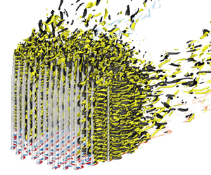
The four wake regimes are: (i) the coupled individual wake (CI), in which the array shear layers are stabilised, and the array wake behind the array is dominated by the element-scale wakes of individual cylinders (figure 5a,e); (ii) the Kelvin–Helmholtz instability wake (KH), where the array shear layers are susceptible to Kelvin–Helmholtz instability and form two rows of KH vortices (figure 5b,f); (iii) the ‘steady + shedding’ wake (SS), in which the two array shear layers remain independent in the steady region, before interacting to result in a von Kármán vortex street downstream (figure 5c,g); and (iv) the vortex street wake (VS), where a von Kármán vortex street forms immediately behind the array (figure 5d,h). As the flow transitions from regime CI through to VS, the formation of element-scale vortices in the wake of individual cylinders is progressively suppressed within the array, coinciding with the increasingly dominant array-scale vortices developed behind the array.

Figure 5. Flow characteristics for four regimes of the array-scale wake. (a–d) Cross-sectional instantaneous flow field (at z/D = 0) from 3-D DNS, visualised by spanwise vorticity  ${\omega _z}d/{U_\infty } = [ - 0.4,0.4]$ for (a) coupled individual wake (CI), (b) Kelvin–Helmholtz instability wake (KH), (c) steady + shedding wake (SS) and (d) vortex street wake (VS). Isosurfaces of ${\omega _x}d/{U_\infty } ={\pm} 0.5$ (coloured by ${\omega _x}$) for (e) CI, (f) KH, (g) SS and (h) VS. The four cases in regimes CI, KH, SS and VS have G/d = 8, 4.5, 2.5, 1.2 and N = 31, 109, 31, 31, respectively. As the flow transitions from regime CI through to VS, the vortex structures behind the array progressively evolve from the element scale to the array scale, and the flow exhibits 3-D features largely behind the array rather than within the array.
Figure 5 shows that the flow exhibits 3-D features and that 3-D flow structures can arise behind individual cylinders or the array depending on the wake regime. For instance, in regime CI (see figure 5a,e), it is seen that 3-D vortices develop in the wakes of cylinders at either side of the array. These vortices will merge and be dissipated rapidly in the near wake of the array as they are convected downstream. As the flow transitions into regime KH (see figure 5b,f), whilst there is no 3-D flow structures forming within the array, the array-scale streamwise vortices form when the two rows of KH vortices, associated with each array shear layer, interact with each other to form a vortex street further downstream. In comparison to regimes CI and KH, the flow in regime SS exhibits relatively weak 3-D flow features (figure 5c,g), occurring where the two array shear layers interact to form vortex shedding. Finally, in regime VS, the porous array behaves similarly to an isolated solid cylinder in terms of the formation of a 3-D von Kármán vortex street immediately behind the array (figure 5d,h).
The distribution of three-dimensionality in the system can be further illustrated by examining the time-mean spanwise kinetic energy, which is defined as
 \begin{equation}{E_z} = \frac{1}{T}\int_0^T {\frac{1}{2}{w^2}/U_\infty ^2\,\textrm{d}t} ,\end{equation}
where T (5000 time units) is the sample duration associated with the fully developed flow and  ${w^2}/U_\infty ^2$ is post-processed on a spanwise-averaged flow field. This quantity has been used previously to check the three-dimensionality in the cylinder wake (e.g. Tong et al. Reference Tong, Cheng, Zhao, Zhou and Chen2014; Jiang et al. Reference Jiang, Cheng, Draper, An and Tong2016).
Whilst in regime CI, non-zero  ${E_z}$ values are distributed behind the array and around a few cylinders in the rear of the array (figure 6a). Alternatively, in regimes KH, SS and VS non-zero ${E_z}$ values are only observed behind the array (figure 6b–d). Clearly, the flow exhibits 3-D features largely behind rather than within the array. This is consistent with figure 5 where the three-dimensionality is visualised by isosurfaces of streamwise vorticity.

Figure 6. Distribution of time-mean spanwise kinetic energy  ${E_z}$ (defined in (3.1)) for an array of 31 cylinders. The four cases are the same as in figure 5: (a) CI, (b) KH, (c) SS and (d) VS. Non-zero ${E_z}$ values are mostly distributed behind rather than within the array, indicating the development of three-dimensionality predominantly behind the array.
Although 3-D structures form within the array in regime CI (figures 6a and 5a), the three-dimensionality of the element-scale wakes is relatively weak at  $R{e_d} = 200$, and this is expected given that this Reynolds number is close to the critical Reynolds number (194) for onset of three dimensionality for an isolated cylinder (Williamson Reference Williamson1996; Jiang et al. Reference Jiang, Cheng, Draper, An and Tong2016). Furthermore, at $R{e_d} = 200$ the maximum difference in the average drag coefficient $\overline {{C_d}} $ for two tandem cylinders across the range of G/d = 1.5–8 is only 1 % (Koda & Lien Reference Koda and Lien2013), which suggests limited influence of element-scale three-dimensionality on the element drag. More importantly, studies have found that around 90 % of the total mean drag is associated with the shear layers attached to the cylinder surface, with less dependence on the flow structure in the far wake (e.g. Fiabane, Gohlke & Cadot Reference Fiabane, Gohlke and Cadot2011). This suggests that the array-scale three-dimensionality behind the array, far from most of element wakes, has limited influence on the element drag.
The influence of three-dimensionality on the drag of a single cylinder near a wall is limited when  ${E_z}$ has magnitude less than or equal to 10−2 (Jiang et al. Reference Jiang, Cheng, Draper and An2017). In the present study, each cylinder is confined by surrounding cylinders. Figure 6 shows that the magnitude of ${E_z}$ within the array is between 10−3 and 10−2 for all the regimes. With reference to Jiang et al. (Reference Jiang, Cheng, Draper and An2017), the three-dimensionality in the system should therefore have limited influence on the total drag force of the array.
To further confirm the applicability of 2-D simulations, a comparison of velocity profiles is made between 3-D and 2-D simulations in figure 7. In the streamwise direction (figure 7a–d), for all the regimes, the streamwise velocity decreases with x/D in the upstream of the array and then continuously decreases throughout the array though some velocity fluctuations are observed due to the flow heterogeneity induced by individual cylinders; downstream of the array, the velocity shows complex variation but eventually increases towards the upstream velocity  ${U_\infty }$. As the flow transitions from regime CI to VS, the transverse profile indicates a larger wake deficit in the array wake (at x/D = 1) (figure 7e–h).

Figure 7. Profiles of time-mean streamwise velocity along  $y = 0$ in 3-D simulations compared with 2-D results: (a) CI, (b) KH, (c) SS and (d) VS. Profiles of time-mean streamwise velocity along $x/D = 1$: (e) CI, (f) KH, (g) SS and (h) VS. Whilst there is good agreement of velocity profiles upstream of and within the array, there are differences in the downstream velocity profiles due to the generation of 3-D flow structures.
Upstream of and within the array  $(x/D \le 0.5)$, there is a good agreement between the streamwise velocity profiles (figure 7a–d), with $\textrm{RMS}{\textrm{E}_\varOmega }$ of $\bar{u}/{U_\infty }$ between 3-D and 2-D simulations of 0.2 %, 0.3 %, 0.8 % and 3.3 % for the four regimes, respectively. This suggests that the flow upstream of and within the array modelled in the 2-D simulation is representative of that in the 3-D simulation.
Downstream of the array (x/D > 0.5), the level of agreement between 3-D and 2-D results depends on the wake regime. In regime CI, the profiles in 3-D and 2-D simulations are in excellent agreement for both streamwise and transverse profiles (see figure 7a,e), respectively with  $\textrm{RMS}{\textrm{E}_\varOmega } = 1.8\,\%$ and 1.0 %. In regimes KH and SS, 3-D and 2-D transverse profiles agree reasonably well (see figure 7f,g), both with $\textrm{RMS}{\textrm{E}_\varOmega }$ less than 3.0 %. However, the 3-D and 2-D streamwise profiles show a similar trend but start to deviate in the KH and SS regimes, with higher $\textrm{RMS}{\textrm{E}_\varOmega } = 12.7\,\%$ and 31.3 %, respectively (figure 7b,c). In regime VS (figure 7d,h), both the 3-D and 2-D streamwise and transverse profiles start to deviate, with $\textrm{RMS}{\textrm{E}_\varOmega } = 33.4\,\%$ and 22.4 %, respectively.
The differences in values of  $\bar{u}/{U_\infty }$ downstream of the array are generated due to the following reasons. Firstly, due to missing turbulent diffusion in the 2-D simulation, the 2-D vortex structures in the array wake persist in strength as they travel downstream (not shown) and hence cause stronger wake entrainment. The streamwise velocity is, in turn, recovered in a faster rate relative to that in the 3-D simulation. This faster rate becomes obvious when large-scale 3-D vortex structures are generated at the wake centreline (comparing figures 7b–d and 5b–d). Furthermore, without vortex stretching 2-D array shear layers are much stronger and interact to form vortex shedding closer to the array (not shown), which hence induces wake entrainment earlier than in the 3-D simulation. This is consistent with earlier recovery of $\bar{u}/{U_\infty }$ in the streamwise profile (see figure 7c,d).
The focus of the present study is arrangement effects on the bulk flow through and bulk drag on the array, which are associated with the variation of element-scale flow and drag characteristics with arrangement (demonstrated later). Therefore, no further attempt was made to demonstrate the differences in the array wake between 2-D and 3-D simulations.
The discussions based on figures 5–7 as a combination suggest that 2-D simulations may be a reasonable tool that helps us increase the resolution of the parameter space in investigating the arrangement effects on the drag on the array elements and the bulk velocity through the array, though caution is needed in interpretation of 2-D array-scale wake.
3.2. Arrangement effects: gap ratio and array-to-element diameter ratio
To interpret the arrangement effects at the element scale, a first step is to understand the element-scale flow and drag characteristics within a finite circular array. Since the array is a combination of multiple lines of cylinders, the scenario of flow past a line of cylinders is studied first.
The key findings of flow past a single line of cylinders from existing literature (Hosseini et al. Reference Hosseini, Griffith and Leontini2020; Zhu et al. Reference Zhu, Zhong and Zhou2021; Eizadi et al. Reference Eizadi, An, Zhou, Zhu and Cheng2022) can be summarised as: (i) the flow evolution along the line is chiefly controlled by G/d when  $R{e_d} \le 200$ and $N \ge 3$; (ii) the flow transitions from shear layer reattachment (SLR) and two-row structure (TRS) occurring at $G/d \approx 3.7$; and (iii) SLR and TRS can cause significant drag reduction to the elements covered by these characteristic flow structures.
Two typical cases at G/d = 2 and 4.5 with N = 11 from 3-D simulations are used to illustrate the two characteristic flow structures and drag reduction mechanisms associated with them (see cross-sectional flow fields in figure 8). The flow for G/d = 2 remains 2-D, while the flow is 3-D for G/d = 4.5 (details are not shown). For G/d = 2 (see figure 8a) the two (positive, negative) separated shear layers from the upstream cylinder reattach on the downstream cylinder from C2 to C3 and SLR develops downstream into regular vortex shedding; these vortices develop a unique pattern downstream where the positive and negative vortices are separated into two parallel rows spanning from C8 to C11, i.e. TRS. For G/d = 4.5 (figure 8b), von Kármán vortices develop from C1; these vortices develop TRS downstream spanning from C2 to C4. Further downstream the flow becomes chaotic.

Figure 8. Flow and drag characteristics of a single line of 11 cylinders for θ = 0° in 3-D DNS. Instantaneous cross-sectional (z/D = 0) flow fields for G/d = 2 (a) and G/d = 4.5 (b). (c) Distribution of drag coefficient along the line. Cylinders with TRS or SLR are marked in dark grey in (a–c).
In the wake of a single cylinder, the primary von Kármán vortices were found to develop downstream into TRS when Ly/Lx > 0.365, where Ly is the cross-wake spacing between centres of positive and negative wake vortices and Lx is the distance between centres of adjacent vortices of the same sign (vortex centre is defined by the maximum of spanwise vorticity  ${\omega _z}d/{U_\infty }$). This threshold has been theoretically identified based on inviscid theory and validated through both experiments (Durgin & Karlsson Reference Durgin and Karlsson1971; Karasudani & Funakoshi Reference Karasudani and Funakoshi1994) and numerical simulations (Thompson et al. Reference Thompson, Radi, Rao, Sheridan and Hourigan2014). In the present study, TRS is similarly developed from primary von Kármán vortices from C1 in a line. Therefore, this threshold Ly/Lx > 0.365 is adopted here to quantitatively classify TRS, with the two length scales Ly, Lx illustrated in figure 8(a).
The distribution of drag coefficient along the line for the two gap ratios are plotted in figure 8(c). It is seen that the cylinders within either SLR (C2, C3, C8–C11 marked in dark grey in figure 8a) or TRS (C2–C4 in figure 8b) have very small drag coefficients relative to other cylinders without these typical flow structures.
Figure 9 illustrates how the characteristic element-scale wake varies with increasing G/d (and hence D/d) for a circular array with a fixed total number of cylinders (N = 109) in 3-D DNS. The element-scale wake structure within a multiple-line array exhibits three flow states: (i) SLR develops for a number of cylinders within an array; (ii) the element-scale wake in the array is characterised by TRS, which covers at least two cylinders within a line; and (iii) over the entire array no downstream cylinders are within a region of TRS or SLR (termed ‘non-covered’, or NOC, here). Two cases with SLR are presented in figure 9(a,b). For (G/d, D/d) = (2, 22.2) (figure 9a), SLR fully occupies the three lines of cylinders in the middle of the array (lines 1−, 0, 1+). The SLR is progressively broken down as the array edges are approached (figure 9a). The resultant wakes of individual cylinders remain steady but form a staggered pattern. The formation of the staggered pattern is attributed to flow diversion towards either side of the array, as indicated by diverging streamlines (figure 9a). At larger G/d = 2.5, SLR can develop downstream into vortex shedding (lines 2−, 1−, 0, 1+, 2+ in figure 9b). With further increases in G/d, it is seen that TRS develops for a number of cylinders (figure 9c). The TRS covers from C3 to C5 in four lines (the filled circles in lines 2−, 1−, 1+, 2+) and up to C6 in the middle line (line 0). Finally, NOC is observed for the array with the largest G/d = 8 (figure 9d), where TRS is confined between C2 and C3 in the three lines (0, 1−, 2−) without covering any downstream cylinder in each line. With increasing G/d, SLR or TRS covers a smaller number of cylinders within a line (see figure 9a–d).

Figure 9. Cross-sectional instantaneous flow field (at z/D = 0) for arrays of 109 cylinders with various gap ratios in 3-D DNS. Cylinder lines are numbered, and the cylinders covered by TRS are marked in dark grey in (c,d), which is classified based on the criterion Ly/Lx > 0.365. With increasing G/d, the extent of elements covered by SLR or TRS over the array is reduced.
Flow transition processes similar to those of a single line of cylinders are observed in multiple-line arrays. A transition from SLR to vortex shedding is seen in both a single line and an array for small gap ratio (figures 8a and 9b); for large gap ratio, a downstream transition from primary vortex to secondary vortex and eventually to a chaotic wake is observed in both the single line and the array. Comparisons of spectra of lift coefficient combined with the instantaneous flow field for the array (G/d = 8, N = 109) with those of the counterpart single-line case are used to demonstrate this (see figure 10). The flow and lift spectra for different lines within the array show similar evolution, such that only lines 0 and 4− are presented for demonstration. The primary frequency dominates the first two cylinders in each line within the array (figure 10a 1,a 2,c 1,c 2). This shows that the von Kármán vortex shed from C1 governs the frequency of the TRS occurring behind C2 (see figure 10b). The secondary frequency emerges on the spectrum of C2 and then becomes dominant over C3 to C6 (figure 10a 3–a 6,c 3–c 6). Further downstream, no dominant frequency is observed (figure 10a 8,c 8), which characterises the chaotic flow (see figure 10b,d). Such downstream evolution of lift spectrum and vortex structures is similar to that for the single line (see figure 10e 1–e 8,f), demonstrating the similarity of flow evolution within the array to that for a single line of cylinders.

Figure 10. Similarity of downstream evolution of the lift coefficient spectrum and instantaneous flow between an array of 109 cylinders and a single line of 11 cylinders (both at G/d = 8) in 3-D DNS. Here ‘P’ and ‘S’ represent primary and secondary frequencies, which are indicative of the element-scale primary vortex and secondary vortex, respectively.
Similarity is also seen in the distribution of drag coefficients of cylinders along the line. This is demonstrated in figure 11 for an array of cylinders with N = 109, G/d = 4.5, for which the instantaneous flow field is shown in figure 9(c). It is seen that the drag distributions along lines of cylinders are very similar to that of the single line especially in the middle of the array (comparing figure 11 with figure 8c), with a sharp decrease of  $\overline {{C_{d,i}}} $ through the first three cylinders, followed by an increase and a decrease over downstream cylinders.

Figure 11. Distribution of drag coefficient of cylinders within an array of cylinders with N = 109, G/d = 4.5 in both 3-D and 2-D DNS. The cross-sectional instantaneous flow field for this case is shown in figure 9(c). The distributions of  $\overline {{C_{d,i}}} $ along the line of cylinders within the array in both 3-D and 2-D simulations are similar to that of the single line of cylinders shown in figure 8(c), especially in the middle of the array, suggesting the applicability of using 2-D DNS in characterising the element drag.
The variation of  $\overline {{C_{d,i}}} $ along each row of cylinders within the array in 2-D simulations follows the trend of that in 3-D simulations. Values of $\overline {{C_{d,i}}} $ for some cylinders in 3-D simulations are slightly lower than those in 2-D simulations. For all the cases in the present study, the $\textrm{RMS}{\textrm{E}_\varOmega }$ for $\overline{C_{d, i}}$ is less than 8 %. This level of discrepancy of $\overline {{C_{d,i}}} $ between 3-D and 2-D simulations is comparable to that of flow past two tandem cylinders (e.g. Reference Koda and LienKoda & Lien 2013). This demonstrates the minor effect of using the 2-D assumption to simulate the flow within the present scope.
Despite the similarity, the presence of the adjacent lines of cylinders in proximity in arrays makes the flow evolution along a line within the array more complicated than that along the single line. The adjacent lines have two effects on the flow: (i) adjacent lines behave similarly to bounding walls (Zdravkovich Reference Zdravkovich1997; Sahin & Owens Reference Sahin and Owens2004) to confine the flow motions in the cross-flow dimension (referred to herein as a confinement effect), and (ii) vortices shed from adjacent lines interact with each other (vortex interaction), destroying the regular vortex structures. The confinement effect is illustrated by comparing the instantaneous flow field between the single line and the lines within the array for the same G/d = 2. For the single-line case (figure 8a), the flow develops downstream from SLR to vortex shedding. In contrast, the flows along three lines within the array (1−, 0, 1+ in figure 9a) are stabilised with SLR persisting throughout the array due to the confinement of adjacent lines of cylinders.
A consequence of adjacent lines is a more chaotic flow within the array, in comparison with that along the single line of cylinders. For a single line of cylinders, a distinct low frequency  $(fd/{U_\infty } = 0.035)$ is observed from C4 to C8 (see figure 10e 4–e 8). This frequency corresponds to the large-scale tertiary vortex reported in Eizadi et al. (Reference Eizadi, An, Zhou, Zhu and Cheng2022). This is, however, absent for the array (figure 10a 4–a 8,c 4–c 8) where the flow exhibits a chaotic shedding feature (see figure 10b,d).
In addition to the influence of adjacent lines, flow through an array is more complex still than that of a single line due to the diversion of flow around the array. With this diverted flow, element wakes (particularly near array edges) are directed laterally towards the edge of the array, as shown by streamlines in figure 9(a). Hence typical flow structures such as SLR and TRS, formed due to the alignment of element wakes with the incident flow, progressively break down as array edges are approached (figure 9a–d). This is the reason why the drag distribution along a line of cylinders in an array increasingly deviates from that of a single line of cylinders when the line is closer to the edge of the array (comparing figure 11 with figure 8c).
The identified characteristic flow structures, SLR and TRS, play important roles in determining  $\overline {{C_d}} $. A plot of $\overline {{C_d}} $ for arrays with N = 31 (figure 12a), combined with the cross-sectional instantaneous flow fields in 3-D simulations for critical G/d (figure 12b–d), is used to demonstrate this. It is seen that with increasing G/d, $\overline {{C_d}} $ generally increases towards an asymptotic value of roughly 0.8 (figure 12a). The variation of $\overline {{C_d}} $ with G/d in 3-D simulations is close to that in 2-D simulations. Therefore, 2-D simulations are employed to increase the resolution with G/d and identify critical values (≈3.3, 7.8) for the transition between different regimes. Despite the general increasing trend, the variation of $\overline {{C_d}} $ with G/d depends on the element-scale flow structure. SLR remains dominant in the range G/d = 1.8–2.7 (figure 12a), with a typical instantaneous flow field shown in figure 12(b). There is therefore little variation of $\overline {{C_d}} $ in this range (figure 12a). Beyond G/d = 2.7, SLR starts to break down. With diminished drag reduction in SLR, the $\overline {{C_d}} $ value increases sharply above G/d = 2.7. With further increase in G/d, TRS begins to dominate the element wake. The extent of cylinders covered by TRS is virtually unchanged over the range G/d = 3.4–4.7, in which the instantaneous flow field is similar to that shown in figure 12(c) and hence the $\overline {{C_d}} $ value stabilises around 0.55. There is a second sharp increase of $\overline {{C_d}} $ from G/d = 4.7 to 8 where with increasing G/d the extent of cylinders covered by TRS in a line is progressively reduced upstream and eventually to only C2 for lines in the middle of the array (see figure 12d). The element wake is in NOC for G/d > 8, causing the near-constant value of $\overline {{C_d}} $ for G/d > 8 (figure 12a). The above interpretation reveals the underlying link between the characteristic flow structure (and its variation with G/d) and the averaged element drag coefficient in finite arrays.

Figure 12. Demonstration of the critical role of element-scale flow structures in determining the average element drag coefficient in both 3-D and 2-D DNS. (a) Variation of  $\overline {{C_d}} $ with G/d for arrays with N = 31. Dashed lines represent the range of G/d where SLR, TRS or NOC become dominant. (b–d) Cross-sectional instantaneous flow fields of N = 31 for critical gap ratios (G/d = 2.7, 4.5, 8) at z/D = 0 in 3-D simulations marked in (a). In (c,d) cylinders covered by TRS are marked in dark grey. Despite the general increasing trend of $\overline {{C_d}} $, values of $\overline {{C_d}} $ are controlled by the characteristic flow structures and its variation with G/d.
More arrays with N = 7, 19, 31, 55, 109 were simulated to demonstrate these three states (SLR, TRS, NOC) in the (G/d, D/d) parameter space (figure 13). This figure includes 10 3-D cases, and 73 complementary 2-D cases due to the computational cost. It is seen from figure 13 that the element-scale wake structures in 3-D and 2-D simulations are in the same flow state for the same value of G/d and D/d. The element-scale wake structure is primarily set by G/d in most cases. For small gap ratio, SLR dominates the element wake within an array at  $G/d\lesssim 3$, whose threshold is less than that for the single line $(G/d\lesssim 3.7)$. For intermediate gap ratio $(3\lesssim G/d\lesssim 8)$, the element-scale wake is characterised by TRS. Cases with large gap ratio $(G/d\gtrsim 8)$ display NOC. With increasing G/d, the transition from SLR into TRS coincides with the decrease in the extent of cylinders within an array covered by SLR, as shown in figure 9(a–c). A similar decreasing trend is observed for the extent of TRS as the flow transitions from TRS to NOC (figure 9c,d). The reduction in the extent of these two characteristic flow structures in an array with increasing G/d is similar to that observed for the single-line scenarios (e.g. Hosseini et al. Reference Hosseini, Griffith and Leontini2020).

Figure 13. The element-scale wake structure and average drag coefficient  $\overline {{C_d}} $ of an array of cylinders mapped out in the parameter space of G/d and D/d for θ = 0° for both 3-D and 2-D DNS. Cases along each dashed line have the same total number of cylinders in the array (N, marked on the right). Cases with the same flow state cluster together, demonstrating dependence of characteristic element-scale flow feature on G/d and D/d. The value of $\overline {{C_d}} $ varies significantly with G/d and D/d from 0.23 to 0.90, highlighting the significant impact of cylinder arrangement.
For a single line (e.g. Eizadi et al. Reference Eizadi, An, Zhou, Zhu and Cheng2022) and an infinite array (da Silva et al. Reference da Silva, Luciano, Utzig and Meier2019) of cylinders, the formation of characteristic element-scale flow features is controlled by the gap ratio when the cylinder Reynolds number is fixed. It appears that this is also the case for a finite circular array when D/d > 10, as shown by the separation of three characteristic element-scale wake states at two virtually invariant G/d values (3, 8) for  $N\gtrsim 31$ in figure 13. This suggests that the array-scale (D/d) has secondary influence on the formation of characteristic element-scale wake if the array has a sufficiently large number of cylinders $(N\gtrsim 31)$ and large size $(D/d\gtrsim 10)$.
Figure 13 also illustrates that the averaged element drag coefficient  $\overline {{C_d}} $ (the filled colour in each symbol) increases with G/d but decreases with D/d, meaning that larger and denser arrays have lower average drag coefficients. The $\overline {{C_d}} $ value varies significantly with G/d and D/d by a factor of more than 4 (from 0.23 to 0.90) in the numerical runs of this study.
3.3. Arrangement effects: incident flow angle
Varying the incident flow angle can generate a wide range of element-scale wake structures, and hence drag distributions, over an array. This is demonstrated through 3-D DNS by varying the incident flow angle for an array of cylinders with N = 31 and G/d = 4.5 in figure 14. For θ = 0°, the flow along each line of cylinders develops from von Kármán vortices into TRS (figure 14a). Channelised flow with streamwise velocity higher than the ambient velocity is formed between adjacent lines (figure 14b). In contrast, the mean velocity in the gap between cylinders in each line is extremely low (figure 14b). The formation of TRS coincides with suppression of lateral mixing (Durgin & Karlsson Reference Durgin and Karlsson1971), which causes the persistence of channelised flow with high velocity throughout the array. The suppression of lateral mixing is indicated by very low Reynolds shear stress magnitude around covered cylinders (marked with dark grey circles in figure 14c). Accordingly, the low gap velocity leads to very low drag force on the cylinders covered by TRS (figure 14d).

Figure 14. The variation with incident flow angle of the fields of cross-sectional instantaneous spanwise vorticity (first row) (at z/D = 0), time-averaged streamwise velocity (second row), Reynolds shear stress (third row) and time-mean force and drag coefficient (fourth row) for an array of 31 cylinders with (G/d, D/d) = (4.5, 24.8) in 3-D DNS. The fields of Reynolds stress and mean flow are post-processed on a time-mean spanwise-average flow field. The first (a–d), second (e–h) and third (i–l) columns represent θ = 0°, 10° and 30°, respectively. Cylinders within the TRS are marked in dark grey in (a,c,e,g). The arrow in the top-right corner of (d,h,l) represents a unit time-mean force of 1. With increasing θ, the TRS in (a) and channelised flow in (b) are progressively suppressed, which creates an increase in mean drag coefficient in (d,h,l).
For the case with θ = 10°, TRS is identifiable in the lower half of the array but completely disappears in the upper half of the array (figure 14e). In the lower half, the flow diversion (towards the lower side) helps to direct the local flow along the geometric channels resulting in the formation of channelised flow. The diverging flow, however, cuts across the channel direction in the upper half and supresses channelised flow, such that most cylinders in the upper half are no longer in the low-velocity wake regions of upstream cylinders (figure 14f). The forces on most of the cylinders are therefore increased and at a significant angle to the primary axis of the line (figure 14h).
For θ = 30°, TRS and channelised flow completely disappear within the array (figure 14i–k), which leads to a significant increase in mean drag coefficient (figure 14l). The flow progressively develops downstream into a chaotic state, as evidenced by the vorticity field in figure 14(i) and the absence of a dominant peak in spectra of lift coefficient (not shown). These chaotic vortices cause stronger lateral mixing in comparison with the other two flow angles (comparing Reynolds shear stress in figure 14c,g,k). Accordingly, the wake deficit of each cylinder is recovered more rapidly than at smaller θ (comparing figure 14b,f,j). Any downstream cylinder is in turn out of the low-velocity region behind its upstream cylinder (figure 14j) and hence has large drag (figure 14l). The resultant average drag coefficient  $\overline {{C_d}} $ increases, more specifically by 42 %, compared with that at θ = 0° (see the legends in figure 14d,l).
The incident flow angle becomes less important with increasing array diameter for a fixed gap ratio. This is illustrated by two arrays with D/d = 24.8 (figure 14) and 48.6 (figure 15) but the same value of G/d (4.5). For  $\theta=0^\circ$, the fraction of elements within TRS decreases from 45 % (figure 14a) to only 14 % when doubling the array diameter (figure 15a). Consistently, the channelised flow is eliminated near the back of the larger array (figure 15a), in contrast to that persisting throughout the smaller array (figure 14b). As indicated by the instantaneous and mean flow fields in figure 15, for the large array, whilst no channelised flow is formed at θ = 30°, a large number of cylinders form chaotic vortex shedding (~39 %, identified from lift coefficient spectra) and are non-channelised for $\theta=0^\circ $. Therefore, when increasing θ from 0° to 30°, the resultant breakdown of TRS and channelised flow impacts fewer cylinders within the larger array.

Figure 15. Cross-sectional instantaneous flow field (upper half) (at z/D = 0) and mean field of streamwise velocity (bottom half) for (a) θ = 0° and (b) θ = 30° in an array of 109 cylinders (G/d, D/d) = (4.5, 48.6) in 3-D DNS. The mean flow is post-processed on a spanwise-average flow field. The colour bar (not shown) of spanwise vorticity is the same as that used in figure 14. Cylinders within TRS are marked in dark grey. With increasing θ from 0° to 30°, the breakdown of TRS and channelised flow impacts relatively fewer cylinders in a large array relative to that in the smaller array in figure 14.
With diminished dominance of TRS and channelised flow, the total drag on the larger array becomes less sensitive to θ. This is best indicated by a transverse-averaged drag coefficient  ${\langle {C_d}\rangle _x}$, in which the angled bracket represents the operation of averaging drag coefficients $\overline{C_{d, i}}$ of elements with identical streamwise (x, denoted in the subscript) but different transverse (y) locations. It is seen that for the smaller array (D/d = 24.8), ${\langle {C_d}\rangle _x}$ for θ = 0° is largely lower than that for θ = 30° (figure 16a). A similar contrast in ${\langle {C_d}\rangle _x}$ is seen in the larger array in the same region of 0 < (x − x 0)/d < 25 (figure 16b), with x 0 the coordinate of the front cylinder in the array. Lower values of ${\langle {C_d}\rangle _x}$ for θ = 0° in both the small and large arrays are associated with the development of channelised flow in the region 0 < (x − x 0)/d < 25 (see figures 14b and 15a). The flow channelisation leads to cylinders in each line largely behaving as a single bluff body and hence imposing smaller drag forces. This difference in ${\langle {C_d}\rangle _x}$ between θ = 0° and 30° is dramatically diminished (and reverses in sign) downstream of (x − x 0)/d = 25 within the larger array (figure 16b). This is because the channelised flow is progressively eliminated beyond (x − x 0)/d = 25 in the large array at θ = 0°, which coincides with cylinders in this region subject to higher local velocity (figure 15a). Near either side of the array where flow diversion is strong, the cylinders beyond (x − x 0)/d = 25 at θ = 0° even experience higher velocity than at θ = 30° (comparing figure 15a,b). This leads to greater $\overline {{C_{d,i}}} $ values for cylinders at (x − x 0)/d > 25 than θ = 30°. This reversal of ${\langle {C_d}\rangle _x}$ at (x − x 0)/d = 25 explains why the averaged drag coefficient $\overline {{C_d}} $ for the larger array is much less dependent on incident flow angle (values provided in figure 16 legends).

Figure 16. Evolution of the transverse-averaged drag coefficient  ${\langle {C_d}\rangle _x}$ along the two arrays for incident flow angles θ = 0° and 30° in 3-D DNS. The two arrays shown in (a,b) have the same value of G/d (4.5) but different values of D/d: (a) D/d = 24.8, N = 31; (b) D/d = 48.6, N = 109. Error bars represent the standard error of the $\overline{C_{d,i}}$ values averaged in the transverse (y) direction. Both arrays have a dependence of ${\langle {C_d}\rangle _x}$ on θ in the region $0 < (x - {x_0})/d < 25$. The larger array has minimal dependence on incident flow angle beyond (x − x 0)/d = 25.
The incident flow angle effects are sensitive to the gap ratio. This is demonstrated by comparing the case of G/d = 2.7 with that of G/d = 4.5 described above. At θ = 0° instantaneous flow within the array is dominated by SLR (figure 17a) and channelised flow develops throughout the array (figure 17b). All cylinders in turn have very low drag except for the most upstream cylinder in each line (figure 17c). Shear-layer reattachment breaks down into vortex shedding for some cylinders for θ = 10° (figure 17d), with incident flow redirected to pass through the gap between adjacent lines of cylinders (figure 17e). For θ = 30°, SLR is completely suppressed, and the flow is characterised by a staggered steady wake pattern (figure 17g). Clearly, with increasing θ, the channel flow is progressively broken down from the top of the array towards its bottom. The average drag coefficient is increased by 15 % with an increase of θ from 0° to 30°, which is smaller than 42 % for the case with G/d = 4.5 (comparing legends between figures 14d,l and 17c,i).

Figure 17. The variation of cross-sectional instantaneous flow field (first row) (at z/D = 0), time-averaged field of streamwise velocity (second row) and the distribution of force and drag coefficient (third row) with incident flow angle for an array of 31 cylinders with (G/d, D/d) = (2.7, 15.3) in 3-D DNS. The first (a–c), second (d–f) and third (g–i) columns represent θ = 0°, 10° and 30°, respectively. The colour bar of spanwise vorticity omitted in (a,d,g) is the same as in figure 14. With increasing θ, SLR in (a) and channelised flow in (b) within the array are progressively suppressed, which coincides with an increase in drag on cylinders over the array in (c,f,i).
In combination, figures 14–17 indicate that the variation of  $\overline {{C_d}} $ with θ is dependent on both the gap ratio and array-to-element diameter ratio. This strong, nonlinear dependence of $\overline {{C_d}} $ on θ is further demonstrated in figure 18 with a combination of 3-D and 2-D simulations. Generally, the influence of incident flow angle on $\overline {{C_d}} $ become less significant with decreasing G/d for a fixed total number of cylinders N. On varying θ from 0° to 30°, the averaged drag coefficient can vary in a wide range. For instance, the $\overline {{C_d}} $ value varies in the ranges of 0.90–1.30 and 0.55–0.78 for the arrays with (G/d, D/d) = (17, 35), (4.5, 24.8), respectively (denoted in order ‘⬠’, ‘□’ in figure 18). All arrays exhibit their lowest value of $\overline {{C_d}} $ at θ = 0° due to the formation of channelised flow at this angle (e.g. figures 14b, 15a and 17b). However, the highest value of $\overline {{C_d}} $ occurs at a range of angles and the averaged drag coefficient does not necessarily increase with θ monotonically. It is therefore insufficient to infer the variation of $\overline {{C_d}} $ with θ based purely on the positioning of cylinders relative to incident flow or the projected area of cylinders normal to the incident flow. The controlling mechanism for the dependence of $\overline {{C_d}} $ on θ is the complex variation of element-scale wake interaction with the cylinder arrangement.

Figure 18. The strong, nonlinear variation of  $\overline {{C_d}} $ with θ across the range of arrays, demonstrating that the $\overline {{C_d}} $ value is not only related to the array geometry but also depends on the orientation of the array. The symbols with red and black edges represent 3-D and 2-D cases, respectively.
3.4. Universal descriptor of bulk flow through a porous array
In §§ 3.2 and 3.3, we have shown that the element-scale flow and drag characteristics can vary widely with arrangement parameters G/d, D/d and θ. However, none of these parameters independently control flow through the porous array. From the perspective of momentum balance, the bulk flow through a porous array is controlled by the array resistance, which is defined by the effective flow blockage parameter  ${\varGamma ^{\prime}_D}$ (Chang & Constantinescu Reference Chang and Constantinescu2015). It is therefore hypothesised that the effective flow blockage parameter provides a universal description of bulk bleeding flow, which is demonstrated in this section.
Figure 19 presents the variation of  ${\bar{u}_p}/{U_\infty }$ with ΓD and ${\varGamma ^{\prime}_D}$, incorporating results from both 3-D and 2-D simulations. The $\textrm{RMS}{\textrm{E}_\varOmega }$ of ${\bar{u}_p}/{U_\infty }$ for the same values of ΓD between 3-D and 2-D simulations is 2 %. Given this small discrepancy, the following discussion is based on a combination of 3-D and 2-D simulations.

Figure 19. The relationship between the bleeding velocity  ${\bar{u}_p}/{U_\infty }$ and flow blockage parameters. Here $\overline {{C_d}} = 1$ and direct measurement of $\overline {{C_d}} $ are used in (a) ΓD and (b) ${\varGamma ^{\prime}_D}$. The filled grey symbols represent the cases varying θ from 0° to 30° with an interval of 5° (see table 4 in Appendix B). The data points are scattered in (a) but collapse well in (b), demonstrating that ${\varGamma ^{\prime}_D}$ controls the bulk bleeding flow.
First, the variation of bulk bleeding velocity  ${\bar{u}_p}/{U_\infty }$, defined in (2.7), with the geometric flow blockage parameter ΓD (assuming $\overline {{C_d}} = 1$) is examined as it has been commonly used to describe the bleeding flow in previous studies (e.g. Rominger & Nepf Reference Rominger and Nepf2011; Zong & Nepf Reference Zong and Nepf2012). It is seen that the bleeding velocity generally decreases with increasing ΓD. As per (2.13), this means that a denser (low G/d), larger (high D/d) array typically has a lower bleeding velocity.
Despite the general decreasing trend, the bleeding velocity is not entirely controlled by ΓD. Data from the same arrays (and thus the same value of ΓD) but with different arrangements are highly scattered, especially in the intermediate range of ΓD. For instance, figure 19(a) incorporates ten typical arrays with different θ from 0° to 30° with a constant increment of 5°, spanning across the investigated ΓD range (see grey filled symbols). The difference between the maximum and minimum of  ${\bar{u}_p}/{U_\infty }$ in the range of θ = 0°–30° is only about 0.02 for a very small or large flow blockage parameter (e.g. ΓD = 0.3, 24.2). In contrast, for a medium ΓD = 1.8, this difference can be up to 0.15, which is one order of magnitude higher than that for very small or very large ΓD. By varying G/d, D/d and θ (between 0°–30°) simultaneously but keeping ΓD = 1.8, the dimensionless velocity difference between the maximal and minimal values can be even 0.28 and the relative difference is 50 % (cases 8 and 33 in table 4 in Appendix B). These demonstrate that the impact of the cylinder arrangement on bleeding flow is most critical in the intermediate range of ΓD, particularly in the range $1\lesssim {\Gamma_D}\lesssim 3$ where the difference between the minimum and maximum of ${\bar{u}_p}$, associated with variation of θ from 0° to 30°, is greater than 10 % of U∞. The high scattering of data demonstrates that the cylinder arrangement can impose a first-order influence on the bleeding flow. The incompleteness of ΓD in defining bleeding flow is because this parameter only defines the geometric bulk blockage of an array without fully incorporating information of arrangement.
The prevalence of the characteristic flow structures appears to be the underlying physical mechanism for the most critical arrangement effects in the intermediate range of ΓD (1–3). It is found that this range of ΓD corresponds to the intermediate range of G/d and D/d where TRS and SLR is the dominant flow feature within an array (see figure 13). With small variation in θ, the extent of TRS or SLR within the array (and the associated reduction in drag) can be greatly enhanced or suppressed. Accordingly,  $\overline {{C_d}} $ (and thus ${\bar{u}_p}/{U_\infty }$) can be particularly sensitive to θ. Outside this range, the flow within the array is characterised by either non-covered element-scale wake (NOC) (low ΓD) or very low local velocity (hence low drag) (high ΓD); the bleeding flow is therefore less dependent on the cylinder arrangement.
Contrastingly, there is excellent collapse of bleeding flow data with the effective flow blockage parameter  ${\varGamma ^{\prime}_D}$ using direct measurement of $\overline {{C_d}} $ (figure 19b). In fact, the scattered data points in the critical range $(1\lesssim {\Gamma_D}\lesssim 3)$ all collapse in the medium range of $0.5\lesssim {\Gamma^{\prime}_D}\lesssim 1.5$ where ${\bar{u}_p}/{U_\infty }$ has higher gradient against ${\varGamma ^{\prime}_D}$ than at the two ends of ${\varGamma ^{\prime}_D}$. Any change to the cylinder arrangement in this range will alter ${\varGamma ^{\prime}_D}$ and hence dramatically change ${\bar{u}_p}/{U_\infty }$. The improved collapse of ${\bar{u}_p}/{U_\infty }$ with ${\varGamma ^{\prime}_D}$ demonstrates the importance of hydrodynamic response of $\overline {{C_d}} $ to the array arrangement in controlling the bulk bleeding flow, which is, however, missed in geometric ΓD. The response is manifested by the variation of element-scale flow and drag characteristics with arrangement as discussed in §§ 3.2 and 3.3. By allowing the controlling influence of array arrangement on $\overline {{C_d}} $, the effective flow blockage parameter, i.e. ${\varGamma ^{\prime}_D}$, not only controls the amount of flow passing through a porous array but also determines when the arrangement effects are critical.
There is vast variability of element-scale flow characteristics in  ${\varGamma ^{\prime}_D}$. For instance, the two 3-D cases 13* and 20* (marked in bold text in table 4) with ${\varGamma ^{\prime}_D} \approx 1.5$ have different element-scale flow structures but almost identical values of ${\bar{u}_p}/{U_\infty } \approx 0.2$. Vortex shedding is formed within one array (G/d = 2.5, D/d = 27.5, N = 109) at θ = 0° but not in the other array (G/d = 2.3, D/d = 13, N = 31) at θ = 30° (see figure 23a,b in Appendix B). The effective flow blockage parameter basically characterises the net bulk resistance of the array, which determines the bulk bleeding flow. The resistance can be broken down into discrete point drag forces, which are physically modelled by individual cylinders in a circular domain herein. Depending on the array and incident flow properties (defined by G/d, D/d, α, θ, Red), the array can have various element-scale flow and drag characteristics at fixed ${\varGamma ^{\prime}_D}$.
Figure 19(b) demonstrates that the bulk bleeding velocity is a function of  ${\varGamma ^{\prime}_D}$. Furthermore, this paper demonstrates the complex variation of $\overline {{C_d}} $, a critical component of ${\varGamma ^{\prime}_D}$, with arrangement, by varying selected arrangement parameters (G/d, D/d, θ) in §§ 3.2 and 3.3. As a combination, this shows how the arrangement changes the element-scale flow and drag characteristics and eventually changes the bulk force on and the bulk flow through the array. The relevance of $\mathit{\Gamma_{D}^{\prime}}$ and coupling between element and array scales are further explored in He et al. (Reference He, Draper, Ghisalberti, An and Branson2024a).
3.5. Variability of averaged drag coefficient
The scattering of data points in figure 19(a) is related to the variation of  $\overline {{C_d}} $ for the same ΓD (geometric flow blockage). By accounting for the $\overline {{C_d}} $ variation, figure 19(b) presents a relation between ${\bar{u}_p}/{U_\infty }$ and ${\varGamma ^{\prime}_D}$. However, prediction of ${\bar{u}_p}/{U_\infty }$ in reality still requires quantitative information of $\overline {{C_d}} $. Therefore, the variability of $\overline {{C_d}} $ in and with ΓD is investigated in figure 20(a), which compiles data from this study and previous work (listed in figure 20b). It is seen that the present data agree with existing data of various arrangements and Red. The $\textrm{RMS}{\textrm{E}_\varOmega }$ of ${\bar{u}_p}/{U_\infty }$ for the same values of ΓD between the present 3-D and 2-D simulations is 8 %.

Figure 20. (a) An integration of data of  $\overline {{C_d}} $ against ΓD from previous studies and the present work. (b) List of references shown in (a). The symbols from the present study represent the same cases as shown in the legend in figure 19(a). Note: Exp, laboratory experiment; Num, numerical simulation. The plot in (a) demonstrates that there is clear variability of $\overline {{C_d}} $ with ΓD, but also scatter across systems.
With increasing ΓD the averaged drag coefficient generally decreases and variability of  $\overline {{C_d}} $ in ΓD reduces. The averaged drag coefficient varies from minimum to maximum by up to 50 % at low ΓD = 0.5, but only by 17 % at ΓD = 24 in the range θ = 0°–30°. For large ΓD, the array can be either very densely packed or very large, which respectively reduces the freedom of altering arrangement and limits the impact of typical flow structures in changing arrangement. The overall drag force in turn becomes much less dependent on arrangement. Instead, it is more dependent on the extremely low bleeding velocity. This leads to convergence of $\overline {{C_d}} $ at high ΓD.
Most data in figure 20(a) have  $\overline {{C_d}} $ values much lower than unity, the value adopted in previous studies (e.g. Zong & Nepf Reference Zong and Nepf2012). While $\overline {{C_d}} = 1$ was assumed with reference to a single solid cylinder in steady flow, the averaged drag coefficient for a porous array is normally lower than that for a single cylinder due to arrangement effects. The complex variation of element-scale flow characteristics with independent variables (G/d, D/d, θ, α, Red) makes it difficult to collapse those independent parameters down to a single parameter to accurately characterise $\overline {{C_d}} $. Nevertheless, figure 20(a) enables a rough estimation of $\overline {{C_d}} $ for real systems, with uncertainty range for given ΓD. When combined with figure 19(b), it provides predictive capacity for the bulk bleeding velocity.
3.6. Fluctuating force characteristics
In previous sections, force characteristics of individual elements have been discussed through time-mean quantities (e.g.  $\overline {{C_d}} $). To show the whole picture of element-scale hydrodynamic features, in this section, the fluctuating components of lift and drag forces are explored. These two components are quantified by the average root mean squares of lift and drag coefficients of individual elements, as defined in (2.5). The $\textrm{RMS}{\textrm{E}_\varOmega }$ of $\overline {{C_{d,rms}}} $ and $\overline {{C_{l,rms}}} $ for the same values of ${\varGamma ^{\prime}_D}$ between the present 3-D and 2-D simulations are 4 % and 10 %, respectively.
The variations of  $\overline {{C_{d,rms}}} $ and $\overline {{C_{l,rms}}} $ with ${\varGamma ^{\prime}_D}$ are associated with both element-scale and array-scale wake structures (figure 21). With an increase of ${\varGamma ^{\prime}_D}$ from 0, the $\overline {{C_{d,rms}}} $ and $\overline {{C_{l,rms}}} $ values increase and peak at ${\varGamma ^{\prime}_D} \approx 1$ and then decrease sharply to approach zero at ${\varGamma ^{\prime}_D} \approx 1.5$. This increasing trend is due to the transition of element-scale wake structure from NOC to TRS state with stronger flow fluctuations within the array. In contrast, beyond ${\varGamma ^{\prime}_D} \approx 1$, the number of cylinders with element-scale vortex shedding is reduced with the increase of ${\varGamma ^{\prime}_D}$ due to lower bleeding velocity and smaller gaps between individual elements. This is responsible for the decrease of $\overline {{C_{d,rms}}} $ and $\overline {{C_{l,rms}}} $ to 0.

Figure 21. The variations of average root mean square lift and drag coefficients with the effective flow blockage parameter. The symbols represent the same cases as shown in the legend in figure 19(a). Note that the dashed ellipses mark the cases 12* and 19* (table 3 in Appendix B), which have different arrangements but the same value of ΓD = 3. The  $\overline {{C_{d,rms}}} $ and $\overline {{C_{l,rms}}} $ values show a different variation with ${\varGamma ^{\prime}_D}$ on either side of ${\varGamma ^{\prime}_D} \approx 1.5$.
In comparison with this decrease, the  $\overline {{C_{d,rms}}} $ and $\overline {{C_{l,rms}}} $ values start to increase when ${\varGamma ^{\prime}_D}\gtrsim 1.5$. Whilst the element-scale vortex shedding is completely suppressed in this ${\varGamma ^{\prime}_D}$ range, the fluctuations of lift and drag forces are driven by flow oscillations induced by the array-scale vortex structures behind the array. The bleeding velocity is reduced with the increase of ${\varGamma ^{\prime}_D}$ such that the array shear layers become much stronger and the location of generating stronger large-scale vortex structures shifts towards the array. This causes stronger oscillations to the flow within the array by changing the pressure in the near wake of the array, which leads to larger fluctuations of lift and drag forces on individual cylinders.
Similar to  $\overline {{C_d}} $ and ${\bar{u}_p}/{U_\infty }$, the $\overline {{C_{d,rms}}} $ and $\overline {{C_{l,rms}}} $ values can also vary widely with the cylinder arrangement, especially in the range of ${\varGamma ^{\prime}_D}\lesssim 1.5$. For instance, through changing the cylinder arrangement (G/d, D/d, θ) but keeping ΓD = 3, both $\overline {{C_{d,rms}}} $ and $\overline {{C_{l,rms}}} $ values can vary by two orders of magnitude (see 3-D data points denoted by dashed ellipses in figure 21a,b). Even considering the same value of ${\varGamma ^{\prime}_D} = 1.2$, the value of $\overline {{C_{l,rms}}} $ can vary by a factor of two (from 0.3 up to 0.6). The effective flow blockage parameter ${\varGamma ^{\prime}_D}$ controls the time-mean bulk flow through the array ${\bar{u}_p}/{U_\infty }$ but not for the instantaneous flow within the array (hence $\overline {{C_{d,rms}}} $ and $\overline {{C_{l,rms}}} $).
4. Discussion
Three-dimensional DNS is used to set the benchmark for this work. Limited by high computational costs, 2-D DNS served as complement to further resolve the parameter space. Using 2-D simulations with removing the complexity of spanwise flow variation allows important element-scale wake interaction patterns on the x–y plane to be identified that are the key for arrangement effects. Although reasonable agreement is seen between 2-D and 3-D results (see figures 7, 11–13, 19–21), 3-D effects exist in most of the cases, mostly in the array wake behind the array (as demonstrated in figures 5 and 6). Therefore, 2-D simulations will not be able to fully characterise wakes of these porous arrays. Since the 3-D effect and turbulence influence will increase with Reynolds number, 2-D DNS is only valid in modelling flow through an array of cylinders at relatively low Reynolds number.
The identification of the controlling influence of arrangement is of practical importance, as real systems, such as aquatic vegetation, foundation piles and offshore structures, typically span the most critical range of  $1\lesssim {\Gamma_D}\lesssim 3$. For instance, kelp forests, seagrasses and emergent marsh grasses have values of ΓD ~ O(0.1–10) (Rominger & Nepf Reference Rominger and Nepf2011). The demonstration of arrangement effects represents a transformation of how to consider the interaction between flow and a porous obstruction with a large number of elements. To understand flow through any given porous obstruction, the orientation of its geometry relative to the incident flow must be known first.
Data from existing literature suggest that arrangement effects are not limited to the range of Reynolds number and array geometry (regular, isotropic configuration of cylinders) investigated in this study. For example, the data in Takemura & Tanaka (Reference Takemura and Tanaka2007) showed that the averaged drag coefficient can be increased by 60 % when varying θ from 0° to 45° for an array with α = 63.4° and Red = 4000. Similar increasing trend of  $\overline {{C_d}} $ is seen in the data in Zhao et al. (Reference Zhao, Cheng, An and Tong2015) with much lower Red = 100. In comparison with these regular arrays, the total drag on a random array can vary by a factor of more than 3, through changing the element arrangement in an array with fixed array diameter (Nair et al. Reference Nair, Kazemi, Curet and Verma2023). All these published results collectively suggest that the arrangement effects still exist for other values of α, Red and random arrays. However, since real systems such as aquatic vegetation can span a wide range of α and Red ~ O(0–10 000) (e.g. Koch et al. Reference Koch, Ackerman, Verduin and van Keulen2007; Tanino & Nepf Reference Tanino and Nepf2008) and elements within it can be randomly distributed, further work is recommended to quantitatively explore the arrangement effects over a wider range of $Re_{d}$ and array geometries.
5. Conclusion
This study investigates and confirms the controlling influence of cylinder (element) arrangement on flow through a circular array of cylinders with DNS, by varying independent dimensionless arrangement parameters, i.e. gap ratio G/d (in the range 1.2–18), array-to-cylinder diameter ratio D/d (3.6–200) and incident flow angle θ (0°–30°) at constant cylinder Reynolds number Red = 200. The geometric flow blockage parameter ΓD, combining the influence of G/d and D/d, spans across the range 0–30. In the parameter space considered here, 3-D DNS results show that the flow exhibits 3-D features largely in the array wake behind the array rather than in element wakes within the array.
We have demonstrated that the complex variation in local flow and drag characteristics of individual cylinders within an array is the mechanism for the arrangement effects on the bulk flow through the array. Element-scale flow structure within an array is therefore characterised across the full range of G/d and D/d. It is found that at fixed θ the element-scale flow structure is chiefly controlled by G/d and the influence of the array scale (D/d) on the formation of characteristic element-scale wake within an array becomes negligible when the array has enough cylinders  $(N\gtrsim 31)$ and large size $(D/d\gtrsim 10)$. Specifically, the element wakes over an array are dominated by SLR and TRS for $G/d\lesssim 3$ and for $3\lesssim G/d\lesssim 8$, respectively. The flow can transition downstream either from SLR to vortex shedding or from primary vortex (including von Kármán vortex, TRS) to secondary vortex and eventually to chaotic wake. These flow transition processes are similar to those observed in flow past a single line of cylinders but with additional complexity due to the influence of adjacent lines of cylinders within the array and flow diversion towards either side of the array. This paper contributes towards linking an understanding of flow through a large array of cylinders with understanding of the flow interaction with a smaller number of cylinders or a single line of cylinders.
For the same ΓD, with varying the cylinder arrangement (by changing G/d, D/d, θ), the averaged drag coefficient  $\overline {{C_d}} $ can vary by up to 52 %, the fluctuating components of lift and drag coefficients $\overline {{C_{d,rms}}} $ and $\overline {{C_{l,rms}}} $ can vary by one order of magnitude and the bulk flow velocity ${\bar{u}_p}$ through an array can be increased by up to a factor of 2 and 30 % of ambient velocity. The arrangement effects on ${\bar{u}_p}$ are most critical at the intermediate range of ΓD (1–3). Particularly, in this range, the difference between the minimum and maximum of ${\bar{u}_p}$, associated with variation of θ in the range 0°−30°, is greater than 10 % of U∞. The reason for the critical range is that the extent of TRS or SLR within the array (and the associated reduction in element drag) can be greatly enhanced or suppressed even with slight change in arrangement (e.g. θ) in this range. It has been demonstrated that the effective flow blockage parameter ${\varGamma ^{\prime}_D}$ using direct measurement of $\overline {{C_d}} $ controls the bulk velocity ${\bar{u}_p}$ across the full range of cylinder arrangements as it allows the controlling influence of array arrangement on $\overline {{C_d}} $. The arrays with the same ${\varGamma ^{\prime}_D}$ can have very different element-scale flow structures within an array but the same ${\bar{u}_p}$. The critical ΓD range (1–3) falls into the intermediate range of ${\varGamma ^{\prime}_D}$ (0.5–1.5) where the arrangement effects are critical.
This paper demonstrates that the modification of bleeding velocity and element-scale wake interaction can be effectively achieved by altering the element arrangement within a porous circular array. Arranging elements within the array to θ = 0° leads to the lowest drag on the array and hence the highest amount of bulk flow passing through it. At this typical θ, the lateral mixing around elements covered by characteristic flow structures (SLR, TRS) is almost fully suppressed. On varying θ to a non-zero degree, the array drag is increased and hence the bulk flow velocity is reduced. However, the maximum drag and the minimum bulk flow velocity can occur at a range of θ between 0° and 30°, depending on the element-scale wake interaction within the array. This provides guidance for the design of engineered structures to maximise or minimise the bulk velocity through them. Furthermore, the demonstration of controlling influence of arrangement in the intermediate range of  ${\varGamma ^{\prime}_D}$ is of practical importance as real systems, such as aquatic vegetation, offshore structures and foundation piles, typically span this range. Finally, the relation of $\overline {{C_d}} $ with ΓD is presented, and it improves our predictive capacity for the bulk bleeding velocity when combined with the universal relation of ${\bar{u}_p}$ with ${\varGamma ^{\prime}_D}$.
Acknowledgements
F.H. would like to acknowledge the support from the Australian Government and the University of Western Australia by providing RTP and UPA scholarships for a doctoral degree. This work was supported by resources provided by the Pawsey Supercomputing Centre with funding from the Australian Government and the Government of Western Australia.
Funding
This research received no specific grant from any funding agency, commercial or not-for-profit sectors.
Declaration of interests
The authors report no conflict of interest.
Appendix A. Numerical validations
A.1. Numerical validation for the case of an isolated cylinder
The numerical scheme was validated by comparing the results of flow past an isolated cylinder in both 2-D and 3-D simulations with those of existing studies (Norberg Reference Norberg2002; Qu et al. Reference Qu, Norberg, Davidson, Peng and Wang2013; Jiang & Cheng Reference Jiang and Cheng2021). Figure 22 compares the distribution of pressure coefficient  ${C_p}$ around the cylinder surface, where ${C_p}$ is defined as ${C_p} = 2(p - {p_\infty })/{U_\infty }$ in which p is the time-averaged kinematic pressure around the cylinder surface and ${p_\infty }$ is the reference kinematic pressure at the inlet boundary. Flow past an isolated cylinder was modelled at two Reynolds numbers, 200 and 1500. Whilst 200 is equal to the cylinder Reynolds number Red defined based on cylinder diameter, 1500 is equal to the array Reynolds number ReD defined by array diameter when the array approaches a solid body. The pressure coefficient distributions from the present 3-D and 2-D simulations are in excellent agreement with existing studies.

Figure 22. Comparison of distributions of pressure coefficient between the present 2-D and 3-D simulations and previous studies. Whilst agreement in (a) validates the resolution of element-scale flow around the individual cylinders, (b) validates the accuracy of resolving the array-scale flow behind the array. (a) Red = 200 and (b) ReD = 1500.
A.2. Mesh dependence for an array of 31 cylinders
The mesh dependence was checked by quantifying the influence of mesh resolution on the statistical parameters, i.e. the mean drag coefficient of the entire array  $(\overline {{C_d}} )$ and of the centre cylinder ( $\overline {{C_{d,16}}} $ and $\overline {{C_{lrms,16}}} $) at (x/D, y/D) = (0, 0) in table 2. The results calculated using meshes 2–4 (with varying Np from 3 to 7 or halving time step $\Delta tU_{\infty}/d$) are in excellent agreement with the corresponding values obtained using the reference mesh 1. This suggests that the reference mesh is adequate for the numerical simulations of the present study.
Table 2. Influence of mesh resolution on force coefficients for N = 31, G/d = 4.5, D/d = 24.8.

Appendix B
Tables 3 and 4 summarise the testing cases.
Table 3. Summary of testing cases. The cases with and without asterisk represent 3-D and 2-D numerical simulations, respectively. Cases simulated with θ = 0°, 5°, 10°, 15°, 20°, 25° and 30° are denoted ‘0°−30°’

Table 4. Summary of testing cases from 3-D and 2-D simulations shown in figure 19. The case numbers correspond to those of table 3. The two cases marked in bold text are cited in § 3.4, with flow fields shown in figure 23. The columns of  ${\varGamma ^{\prime}_D}$ and ${\bar{u}_p}/{U_\infty }$ are denoted with text only for θ = 0°.


Figure 23. Comparison of instantaneous flow fields between two cases with  ${\varGamma ^{\prime}_D} = 1.5$ but different arrangements. Vortex shedding is observed within the large array in (a) but not for the small array in (b). (a) (G/d, D/d, N, θ) = (2.5, 27.5, 109, 0°) and (b) (G/d, D/d, N, θ) = (2.3, 13, 31, 30°).


 Open access