


Crossref Citations
This article has been cited by the following publications. This list is generated based on data provided by Crossref.
Cavalieri, André V. G.
Jordan, Peter
and
Lesshafft, Lutz
2019.
Wave-Packet Models for Jet Dynamics and Sound Radiation.
Applied Mechanics Reviews,
Vol. 71,
Issue. 2,
Brès, Guillaume A.
and
Lele, Sanjiva K.
2019.
Modelling of jet noise: a perspective from large-eddy simulations.
Philosophical Transactions of the Royal Society A: Mathematical, Physical and Engineering Sciences,
Vol. 377,
Issue. 2159,
p.
20190081.
Tuttle, Steven G.
Fisher, Brian T.
Kessler, David A.
Pfützner, Christopher J.
Jacob, Rohit J.
and
Skiba, Aaron W.
2021.
Petroleum wellhead burning: A review of the basic science for burn efficiency prediction.
Fuel,
Vol. 303,
Issue. ,
p.
121279.
Bonelli, Francesco
Viggiano, Annarita
and
Magi, Vinicio
2021.
High-speed turbulent gas jets: an LES investigation of Mach and Reynolds number effects on the velocity decay and spreading rate.
Flow, Turbulence and Combustion,
Vol. 107,
Issue. 3,
p.
519.
Volpiano, Riccardo
and
Maffiodo, Daniela
2023.
Advances in Mechanism and Machine Science.
Vol. 148,
Issue. ,
p.
226.
Maffiodo, Daniela
and
Volpiano, Riccardo
2024.
Optimization of Customized Industrial Pneumatic Nozzle to Reduce Noise Emissions.
Applied Sciences,
Vol. 14,
Issue. 3,
p.
981.
1 Introduction: The challenge of jet noise prediction
Jet exhausts on aircraft seem tremendously loud, but to understand the challenge of predicting their noise we must not forget that our ears are also remarkably sensitive. The energy of the sound field is minuscule: radiated pressure fluctuations are dwarfed by those in the jet turbulence. As such, sound is easily lost in models or simulations, much as a needle in a haystack, which makes prediction a challenge.
The reason for this acoustic inefficiency is that most of the turbulence does not radiate. Without external mass or momentum sources, turbulence as an acoustic source is nearly self-cancelling. In the zero-Mach-number limit, it is famously quadrupole (Lighthill Reference Lighthill1952), a character that persists up to the near-sonic exit velocities of most civilian transport aircraft. Because the acoustic wave equation does not support waves for subsonic phase velocities, a turbulent eddy that advects unchanged lacks a frequency–wavenumber makeup that would let it radiate sound. Only its evolution as it advects can lead to radiation (Crighton Reference Crighton1975), so sound leaks out only via the energetically minor mechanisms that violate Taylor’s hypothesis.
Given this fundamental challenge, statistical turbulence models for nominal sound sources work admirably well, although they often lack the fidelity needed to meet the needs of engineering design. Seeking sub-decibel (sub-dB) predictive fidelity to design aircraft within noise regulations, many have turned to simulations that include explicit representation of at least the larger turbulence scales. The same near-cancellation of acoustic sources also makes these challenging, since both numerical and physical-modelling errors can lead to spurious sound. It was about 20 years ago that this author had the pleasure of working on some of the first such simulations (Freund Reference Freund2001); simulations such as by Brès et al. (Reference Brès, Jordan, Jaunet and Le Rallic2018) leave those far behind in every regard.
2 Overview: models to achieve predictive performance
The overarching achievement of the present paper is the remarkable agreement with experimental data for a truly turbulent Reynolds number $Re\approx 10^{6}$
laboratory jet. It is carefully evaluated for both far-field sound, achieving the sub-dB fidelity needed for design, and near-field turbulence. All the more remarkable is that by today’s standards these are modest-scale simulations. A combination of adaptive meshing and judiciously adjusted numerical dissipation provides predictive fidelity with just under
$Re\approx 10^{6}$
laboratory jet. It is carefully evaluated for both far-field sound, achieving the sub-dB fidelity needed for design, and near-field turbulence. All the more remarkable is that by today’s standards these are modest-scale simulations. A combination of adaptive meshing and judiciously adjusted numerical dissipation provides predictive fidelity with just under $16\times 10^{6}$
mesh cells. This is less than was used for the first direct numerical simulations of low-
$16\times 10^{6}$
mesh cells. This is less than was used for the first direct numerical simulations of low- $Re$
jets. Many of the mesh cells are smaller, which necessitates smaller time steps, but still only approximately a factor of 10 more time steps are necessary. The judicious meshing and flexible numerical methods facilitate this achievement, though used alone these would be insufficient. The real contribution of this paper is the identification of a mix of physical models in addition to the numerical methods. Doubling the mesh in each direction does not substantively improve predictions without the models.
$Re$
jets. Many of the mesh cells are smaller, which necessitates smaller time steps, but still only approximately a factor of 10 more time steps are necessary. The judicious meshing and flexible numerical methods facilitate this achievement, though used alone these would be insufficient. The real contribution of this paper is the identification of a mix of physical models in addition to the numerical methods. Doubling the mesh in each direction does not substantively improve predictions without the models.
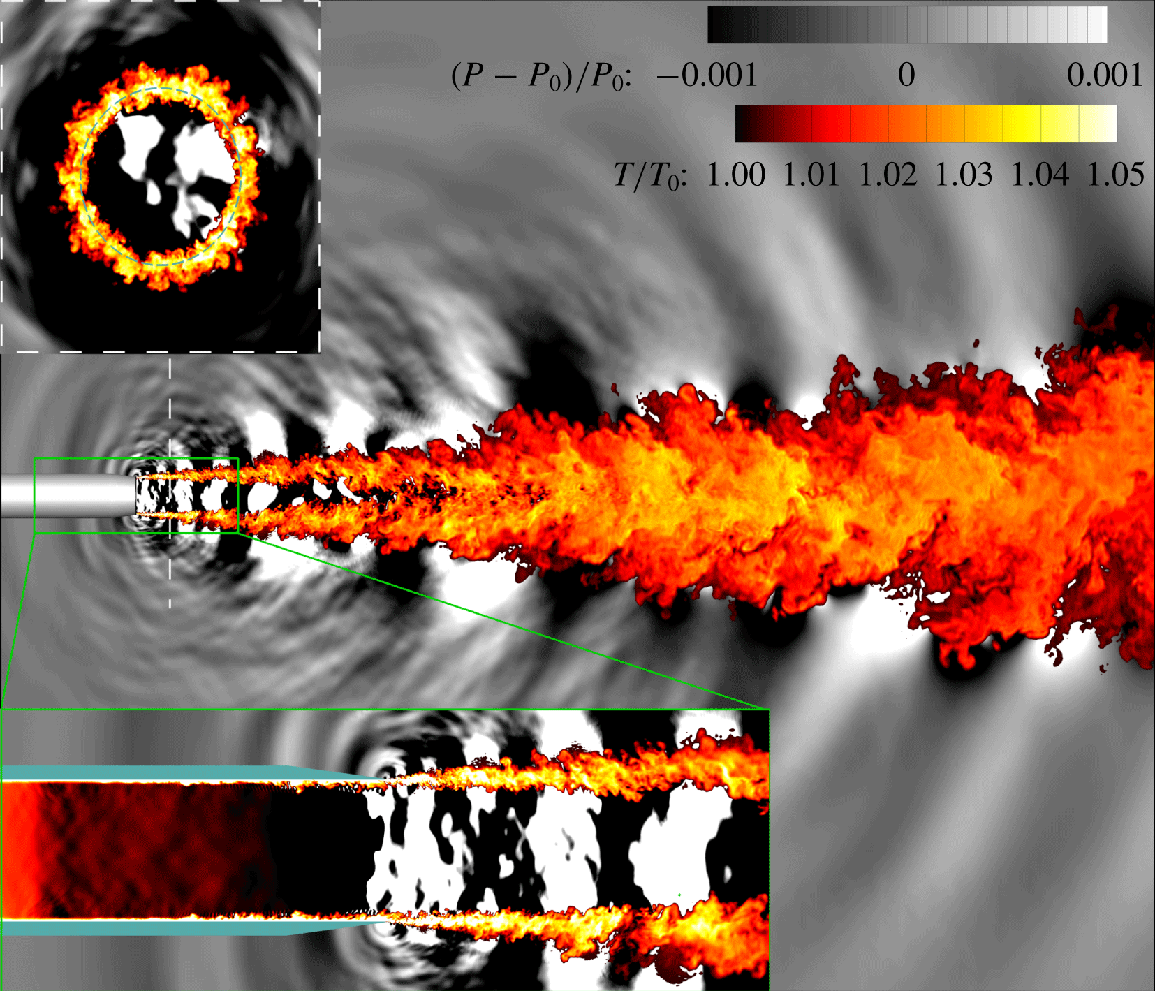
The main challenge is representing the near-nozzle shear layers, which develop from boundary layers on the inner wall of the nozzle. Contractions upstream of the nozzle exit plane make these remarkably thin (see figure 1), with $\unicode[STIX]{x1D6FF}<0.01D$
. The authors use adaptive meshing to resolve the turbulence both in the
$\unicode[STIX]{x1D6FF}<0.01D$
. The authors use adaptive meshing to resolve the turbulence both in the $D$
-diameter jet and in the
$D$
-diameter jet and in the $\unicode[STIX]{x1D6FF}$
-scale near-nozzle shear layers. This is particularly important, because despite the scale mismatch, jet noise is sensitive to the turbulence in this thin layer. Laminar shear layer jets are louder (Zaman Reference Zaman2012), and even when the initial shear layers are turbulent, the radiation still depends upon
$\unicode[STIX]{x1D6FF}$
-scale near-nozzle shear layers. This is particularly important, because despite the scale mismatch, jet noise is sensitive to the turbulence in this thin layer. Laminar shear layer jets are louder (Zaman Reference Zaman2012), and even when the initial shear layers are turbulent, the radiation still depends upon $\unicode[STIX]{x1D6FF}$
even for
$\unicode[STIX]{x1D6FF}$
even for $\unicode[STIX]{x1D6FF}\ll D$
(Fontaine et al.
Reference Fontaine, Elliott, Austin and Freund2015). Early simulations of jets avoided the nozzle altogether, and specified perturbed laminar profiles (e.g. Freund Reference Freund2001), which is only true at uncommonly low Reynolds numbers, or turbulent but artificially thick. Bailey and Bogey and co-authors (e.g. Bogey & Bailly Reference Bogey and Bailly2010) have studied the sensitivity to inflow conditions in simulations with nozzles, and more recently they have used very large meshes (
$\unicode[STIX]{x1D6FF}\ll D$
(Fontaine et al.
Reference Fontaine, Elliott, Austin and Freund2015). Early simulations of jets avoided the nozzle altogether, and specified perturbed laminar profiles (e.g. Freund Reference Freund2001), which is only true at uncommonly low Reynolds numbers, or turbulent but artificially thick. Bailey and Bogey and co-authors (e.g. Bogey & Bailly Reference Bogey and Bailly2010) have studied the sensitivity to inflow conditions in simulations with nozzles, and more recently they have used very large meshes ( ${>}3\times 10^{9}$
points) to meet this challenge (Bogey & Marsden Reference Bogey and Marsden2016). It is this set of long-standing challenges that the present paper has met with modest computational expense.
${>}3\times 10^{9}$
points) to meet this challenge (Bogey & Marsden Reference Bogey and Marsden2016). It is this set of long-standing challenges that the present paper has met with modest computational expense.
Figure 1. Simulation of Brès et al. (Reference Brès, Jordan, Jaunet and Le Rallic2018) illustrating the thinness of the boundary layers within the nozzle where novel modelling facilitates these simulations, the richness of the turbulence in the near-nozzle mixing layers, and the relatively large extent of the jet.
They include the nozzle in the simulation, with the domain inflow $3D$
upstream of the exit plane, and establish independence of both the particular artificial fluctuations used to seed the inflow turbulence and the numerical resolution. Computational cost is low because the boundary layer is only coarsely represented, with
$3D$
upstream of the exit plane, and establish independence of both the particular artificial fluctuations used to seed the inflow turbulence and the numerical resolution. Computational cost is low because the boundary layer is only coarsely represented, with $\unicode[STIX]{x0394}y$
over 100 times that needed to fully resolve all scales. To avoid the consequences of this modest resolution, they use a wall model based on time-averaged (RANS) governing equations. The main conclusion is that all three model components are important, with the wall model the most important, seemingly because it maintains the boundary layer thickness in a way that allows the turbulence fluctuations that are consequential to the near-nozzle shear layers and sound to develop. Free-shear flows, even when they are turbulent, are well known to share features with linear stability modes. Exposing realistic amplitude disturbances to amplification mechanisms for the nearly correct mean flow seems to be what the authors have accomplished. Of the two, the results suggest that the turbulence intensity is particularly important: their model that yields the best sound predicts turbulence intensity more closely than mean flow profile.
$\unicode[STIX]{x0394}y$
over 100 times that needed to fully resolve all scales. To avoid the consequences of this modest resolution, they use a wall model based on time-averaged (RANS) governing equations. The main conclusion is that all three model components are important, with the wall model the most important, seemingly because it maintains the boundary layer thickness in a way that allows the turbulence fluctuations that are consequential to the near-nozzle shear layers and sound to develop. Free-shear flows, even when they are turbulent, are well known to share features with linear stability modes. Exposing realistic amplitude disturbances to amplification mechanisms for the nearly correct mean flow seems to be what the authors have accomplished. Of the two, the results suggest that the turbulence intensity is particularly important: their model that yields the best sound predicts turbulence intensity more closely than mean flow profile.
3 Future
This paper is, in a sense, an endpoint. The authors reproduce laboratory flows and sound with unprecedented accuracy, sufficient for most engineering, and they do this with tractable computational cost. Yet, it is also just a step towards solving the real problems. On tarmacs worldwide one sees that the newest nozzle lips are serrated with regular chevron features. Can their sound be predicted with this same fidelity and modest cost for extrapolative design? In forward flight, there will also be a turbulent boundary layer exterior to the nozzle, so understanding any additional mechanisms it introduces and modelling them will also demand attention. A perhaps greater challenge will be to move from the high-contraction-ratio isentropically compressed uniform core flows of most laboratory jets, to the combustion products and unsteadiness of jet engines. All such complexities will require additional analysis, model development well grounded in turbulence mechanics, and multi-quantity evaluation against high-quality data.
A longer-term question is how to best use such predictions. One route towards this might be to use them to achieve sufficient understanding of mechanisms to guide noise-reduction strategies. Informed by successful predictions, wave-packet models based on the growth and decay of disturbances in the jet might provide a framework for this (Jordan & Colonius Reference Jordan and Colonius2013). These models illuminate mechanisms by which characteristics of the large-scale turbulence are reflected in the far-field sound. They may also prove useful in reduced-order models of radiation and to inspire noise-control techniques, but they are not yet predictive, and it is unlikely they would ever achieve the kind of sub-dB prediction of the radiated sound now achieved with large-eddy simulation. An alternative approach is to directly use inverse methods together with large-eddy simulation to point the way towards noise reduction (e.g. Freund Reference Freund2011). I am personally more optimistic about the latter approach, as it includes all mechanisms including subtle ones that may elude reduced-order modelling. In the end, though, there is significant space for improvement regardless of the specific approach.
One technical challenge, which might be important for engineering and an interesting modelling challenge of itself, would be to increase the frequency of the sound that is accurately predicted. The maximum accurate Strouhal number for the present simulations is $St\approx 2$
. This frequency is consistent with the mesh scale of the simulations (which further supports that the mesh is used efficiently). However, higher-frequency components receive significant weighting based on human perception. Increasing the mesh is the brute force way to expand this range. The approximately double-density mesh in the present paper (at approximately 16 times the computational cost) expands accuracy to
$St\approx 2$
. This frequency is consistent with the mesh scale of the simulations (which further supports that the mesh is used efficiently). However, higher-frequency components receive significant weighting based on human perception. Increasing the mesh is the brute force way to expand this range. The approximately double-density mesh in the present paper (at approximately 16 times the computational cost) expands accuracy to $St\approx 4$
. This general trend seems to persist; with their
$St\approx 4$
. This general trend seems to persist; with their $3\times 10^{9}$
points, Bogey & Marsden (Reference Bogey and Marsden2016) achieve good agreement up to
$3\times 10^{9}$
points, Bogey & Marsden (Reference Bogey and Marsden2016) achieve good agreement up to $St\approx 8$
. There are likely opportunities to develop models for the high-frequency sound, perhaps by revisiting earlier such efforts (e.g. Bodony & Lele Reference Bodony and Lele2003), now with a firmer simulation platform to build upon.
$St\approx 8$
. There are likely opportunities to develop models for the high-frequency sound, perhaps by revisiting earlier such efforts (e.g. Bodony & Lele Reference Bodony and Lele2003), now with a firmer simulation platform to build upon.
Finally, I want to emphasize, that the Brès et al. results do not invoke significant empiricism. Instead, they were achieved with thoughtful analysis, careful simulations, and rigorous comparisons that respect the turbulence mechanics. Empirical spectra can fit data far better than might be expected (e.g. Tam et al. Reference Tam, Viswanathan, Ahuja and Panda2008), which is fascinating and may speak to the underlying mechanisms, but such fits offer no guarantee for extrapolative engineering prediction, and reliance on them for prediction is a step away from advancing true understanding.