


1. Introduction
The ubiquitous free-surface boundary layers in nature are of great importance, primarily in the contexts of mixing, heat/gas transfer, biological activity in the uppermost layer of the ocean and for pollutant dispersion and transport (e.g. Soloviev & Lukas Reference Soloviev and Lukas2013). Dynamics of such boundary layers is usually modelled employing the constant stress boundary condition at the fluid surface, that yields the no-stress condition for perturbations. Free-surface boundary layers were studied experimentally in wind-wave laboratory facilities (e.g. Dupont & Caulliez Reference Dupont and Caulliez1993) and small-scale natural reservoirs. Although oceanic free-surface boundary layers are, as a rule, turbulent, the turbulence is most often modelled by using scalar eddy viscosity, either depth dependent or constant. Very often these boundary layers are density stratified because of direct solar heating or/and air bubble entrainment caused by breaking wind waves (e.g. Terrill, Melville & Stramski Reference Terrill, Melville and Stramski2001; Grimshaw et al. Reference Grimshaw, Khusnutdinova, Ostrovsky and Topolnikov2010; Soloviev & Lukas Reference Soloviev and Lukas2013). Here, we examine the nonlinear dynamics of no-stress boundary layers in very common, but completely overlooked situations of weak density stratification. Even the linear dynamics of such motions has not been studied yet.
As a possible route to mixing in linearly stable free-surface boundary layers we are primarily interested in the nonlinear dynamics of essentially three-dimensional (3-D) long-wave perturbations which are decaying in the linear setting. There were no studies of the nonlinear dynamics in weakly stratified boundary layers. Here, we address this gap and show the principal importance of accounting for even very weak stratification for 3-D perturbations. For strongly stratified boundary layers in an ideal fluid, the models describing the weakly nonlinear one-dimensional dynamics of long-wave perturbations have been known for more than four decades: Maslowe & Redekopp (Reference Maslowe and Redekopp1980) derived the one-dimensional Benjamin–Ono equation for perturbations of a thin strongly stratified layer modified by the account of weak stratification in the bulk of the fluid. Most of the studies of stratified shear flows are concerned with either internal gravity waves of larger scales penetrating the entire water column and usually described by the Korteweg–de Vries (KdV)-type equations (e.g. Apel et al. Reference Apel, Ostrovsky, Stepanyants and Lynch2007) or linear stability analysis of parallel flows, primarily in the inviscid setting, see e.g. reviews in Turner (Reference Turner1979), LeBlond & Mysak (Reference LeBlond and Mysak1981) and Carpenter et al. (Reference Carpenter, Tedford, Heifetz and Lawrence2011). There is also a separate group of studies of ring waves with and without shear and their generalizations (see e.g. Tseluiko et al. (Reference Tseluiko, Alharthi, Barros and Khusnutdinova2023) and references therein). However, as we show below, by ignoring weakly stratified boundary layers a number of interesting and important phenomena have been overlooked.
There is also a corpus of works concerned with non-stratified zero-stress boundary layers which is nevertheless highly relevant for the present study. Consideration of essentially 3-D nonlinear long-wave perturbations in the no-stress boundary layers was originated in Shrira (Reference Shrira1989) in the context of upper ocean. To describe weakly nonlinear evolution of such perturbations in the horizontally uniform boundary layer adjacent to the ocean surface an essentially two-dimensional (2-D) generalization of the Benjamin–Ono (2-D-BO) equation was derived. This equation describes evolution of horizontal spatial structure of perturbations. The dependence of the perturbations on the vertical coordinate splits off and is determined, to leading order, by the corresponding linear boundary value problem. The key assumptions in the asymptotic derivation are the smallness of nonlinearity characterized by a nonlinearity parameter  $\varepsilon \ (\varepsilon \ll 1)$ and the balancing weakness of dispersion due to $O(\varepsilon )$ smallness of the characteristic wavenumber compared with the inverse of the boundary-layer thickness. A perturbation of comparable streamwise and spanwise scales represents a broadband packet of ‘vorticity waves’. In the absence of instability and nonlinearity such a packet is dispersing and decaying. However, the account of nonlinearity radically changes the picture: D'yachenko & Kuznetsov (Reference D'yachenko and Kuznetsov1995) showed that within the framework of the 2-D-BO equation initially localized 2-D perturbations can become infinite in finite time evolving into a point singularity.
A more refined derivation of the 2-D-BO equation and its generalization for the finite depth fluid with arbitrary density stratification outside the homogeneous boundary layer was carried out in Voronovich, Shrira & Stepanyants (Reference Voronovich, Shrira and Stepanyants1998). In the original derivation of the 2-D-BO equation in Shrira (Reference Shrira1989) for the ideal fluid there is a non-uniformity in the asymptotic expansion: the higher-order terms diverge in the critical layer. At a hand waving level it was argued that the account of viscosity would eliminate the singularities. This was indeed elaborated in Voronovich et al. (Reference Voronovich, Shrira and Stepanyants1998) for the case of no-stress boundary: the range of Reynolds numbers was chosen in such a way that viscous effects, on the one hand, are strong enough to eliminate the singularities, while, on the other hand, weak enough not to contribute into the evolution equation and keep the 2-D-BO equation intact. In Shrira, Caulliez & Ivonin (Reference Shrira, Caulliez and Ivonin2005), a generalization of the 2-D-BO equation was derived to model laminar–turbulent transition in the accelerating Falkner–Skan boundary layer; on its basis numerical simulations of the perturbation evolution were carried out and experimental observations of the laminar–turbulent transition in the wind-driven steady boundary layer in water were presented and discussed.
In this work we focus on examining main implications of taking into account two new factors: (i) weak stratification in the boundary layer and (ii) consideration of a wider range of the Reynolds numbers. The main questions we want to address are whether the account of weak stratification can change qualitatively the nonlinear dynamics of 3-D long-wave perturbations and, if yes, what these qualitative changes are. We also aim to clarify the outstanding issue regarding the role of weak dissipative effects both for the weakly stratified and homogeneous boundary layers: a priori it is not known whether and when the account of weak dissipation is qualitatively important. It is highly desirable to have a relatively simple mathematical model systematically and transparently derived from the Navier–Stokes equations which, on the one hand, would allow substantial analytical advance, while, on the other hand, could serve as a starting point for direct numerical simulations further clarifying the fundamental outstanding questions like laminar–turbulent transition. The novel evolution equation we derive aims to address this need.
The derivation and study of nonlinear evolution equations describing various physical phenomena has grown into a field of its own right (e.g. Ablowitz Reference Ablowitz2011; Saut Reference Saut2013). Most of the known nonlinear evolution equations for long waves are derived by balancing weak nonlinearity and weak dispersion for a particular mode, which for long waves usually leads to the KdV/Benjamim–Ono-type equations and their generalizations (e.g. Whitham Reference Whitham2011; Ostrovsky et al. Reference Ostrovsky, Pelinovsky, Shrira and Stepanyants2015). Here, focusing on a particular example of the shear flow dynamics, we put forward an approach which combines conventional long-wave-type expansion with taking into account a weak non-resonant effect of other modes of motion apart from the one we consider. The key underpinning technical trick is to consider concurrently with the standard long-wave expansion an asymptotic expansion in powers of a small parameter characterizing a different physical factor not related to the wavelength scale, and then focus on the distinguished limit. Here, this physical factor is weak density stratification. This changes dispersion qualitatively and thus enables us to extend significantly the class of resulting nonlinear evolution equations, which is of independent interest. In this work we just indicate and then leave aside numerous possible extensions based upon this idea, while concentrating on the particular case of a weakly stratified shear flow dynamics.
The overall picture of dispersion curves of the linear boundary value problem for stratified boundary layers in the case of large Reynolds numbers and small wavenumbers is relatively well understood. Apart from the infinite number of internal gravity modes slightly modified by shear and viscosity, there is also a much less known single ‘vorticity mode’ perturbed by stratification and viscosity; there are also viscous modes strongly localized near the boundary. Here, we focus on the nonlinear evolution of the vorticity mode. In the linear setting the vorticity modes are usually decaying. Although linear instabilities of such modes are also possible, here, we confine our attention to the nonlinear dynamics of linearly decaying perturbations.
The scaling we adopt to derive the evolution equation ensures a ‘distinguished limit’: we balance the effects of weak nonlinearity, weak dispersion independent of stratification, weak dispersion due to stratification and viscous dissipation. That is, on characterizing the smallness of nonlinearity by  $\varepsilon \ (\varepsilon \ll 1)$, we assume the characteristic streamwise and spanwise wavevector components both to be $O(\varepsilon )$, which ensures weakness of the stratification independent Benjamin–Ono-type dispersion. We also adopt a particular scaling of $\varepsilon$ in terms of the Reynolds number ${Re}$ (or an effective Reynolds number in case of eddy viscosity parameterization of a turbulent boundary layer): $\varepsilon \sim {Re}^{-1/2}$. The presumed weakness of stratification is characterized by the $O(\varepsilon )$ smallness of the Richardson number $Ri$, where the Richardson number is defined as the squared ratio of the maximal buoyancy frequency ( $N$) to the maximal shear ( $|U^{\prime }|$). Although the shear flows with the Richardson number below 1/4 are often considered to be a priori unstable, the inequality $Ri<1/4$ is just a necessary condition for the linear instability in the inviscid setting and not a sufficient one (see e.g. Howard Reference Howard1961; Miles Reference Miles1961; Turner Reference Turner1979; LeBlond & Mysak Reference LeBlond and Mysak1981); in nonlinear inviscid theory the instability criterion $Ri<1$ was put forward by Abarbanel et al. (Reference Abarbanel, Holm, Marsden and Ratiu1984), but the picture is not entirely clear. In our consideration here the linear instabilities play no role. In our context the weakness of stratification characterized by the smallness of the Richardson number controls a weakness of a different, and very peculiar, type of dispersion with frequency not dependent on wavenumber. This new dispersion affects only 3-D perturbations and, to the best of our knowledge, has not been reported in the literature.
Starting with the Navier–Stokes equations for an incompressible stratified fluid with constant viscosity, we, by means of the triple-deck asymptotic scheme, derive a novel  $(2+1)$-dimensional evolution equation governing dependence of the vorticity mode amplitude on the horizontal coordinates and time. The equation is an essentially 2-D pseudo-differential nonlinear equation with explicit account of stratification and shear in the boundary layer
 \begin{equation} A_{\tau}+ AA_{x}-\hat{G}_{1}[A_{x}]-\tilde{\beta}_{2}\hat{G}_{2}[A_{x}]+\tilde{\gamma}A=0, \end{equation}
where  $A(x,y,\tau )$ is the amplitude of the streamwise velocity component dependent on the streamwise and spanwise variables, $x,y$ and time, the non-local operators $\hat {G}_{1}$ and $\hat {G}_{2}$ are
 $$\begin{gather} \hat{G}_{1}[\varphi(\boldsymbol{r})]=\frac{1}{4{\rm \pi}^{2}} \int_{-\infty}^{+\infty}\int_{-\infty}^{+\infty}|\boldsymbol{k}| \varphi(\boldsymbol{r}_{1})\exp({-{\rm i}\boldsymbol{k}(\boldsymbol{r}-\boldsymbol{r}_{1})}) \,\mathrm{d}\boldsymbol{k}\,\mathrm{d}\boldsymbol{r}_{1}, \end{gather}$$
 $$\begin{gather}\hat{G}_{2}[\psi(\boldsymbol{r})]=\frac{1}{4{\rm \pi}^{2}} \int_{-\infty}^{+\infty}\int_{-\infty}^{+\infty} \frac{{k_{y}}^{2}}{k_{x}^{2}}\psi(\boldsymbol{r}_{1}) \exp({-{\rm i}\boldsymbol{k} (\boldsymbol{r}-\boldsymbol{r}_{1})})\,\mathrm{d} \boldsymbol{k}\,\mathrm{d}\boldsymbol{r}_{1}. \end{gather}$$
Here, 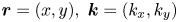 $\boldsymbol {r}= (x,y),\ \boldsymbol {k}= (k_x,k_y)$ is the wave vector, $\phi$ and $\psi$ are arbitrary scalar functions, operator $\hat {G}_{1}[\varphi (\boldsymbol {r})]$ describes the dispersion in the 2-D-BO equation. Sometimes more convenient might be its alternative representation in terms of hypersingular Cauchy–Hadamard integral
 \begin{equation} \hat{G}_{1}[\varphi(\boldsymbol{r})]=\frac{1}{2{\rm \pi}} \int_{-\infty}^{+\infty}\int_{-\infty}^{+\infty} \frac{\varphi(\boldsymbol{r}_1)\,\mathrm{d}\boldsymbol{r}_1} {|\boldsymbol{r} -\boldsymbol{{r}_1}|^{3}}. \end{equation}
 Throughout the paper all improper integrals we encounter are understood as the Hadamard finite-part integrals. Operator  $\hat {G}_{2}[\psi (\boldsymbol {r})]$ describes the ‘new’ dispersion due to weak stratification. The term $\tilde {\gamma }A$ captures the effect of finite Reynolds number describing it as a Rayleigh-type friction, $\tilde {\gamma }\sim U^{\prime \prime \prime }(0)/Re_{\ast }(U^{\prime }(0))^{2}$ is thus proportional to the curvature of vorticity $U^{\prime }$ at the surface. Hence, for the shear profiles where $\tilde {\gamma }<0$, this term describes linear instability. However, here, we confine our attention only to the linearly stable situations, while the linearly unstable ones will be considered elsewhere. Coefficient $\tilde {\beta }_{2}$ is determined by the strength of the stratification at the surface and vanishes in the limit of zero stratification. The corresponding linear dispersion relation in the frame of reference moving with the water surface reads
 \begin{equation} \omega(\boldsymbol k)={-}|\boldsymbol k|- \tilde{\beta}_{2} \frac{k_y^2}{k_x^2} -{\rm i}\tilde{\gamma}. \end{equation}
Although the evolution equation depends only on the horizontal coordinates and time, the model provides the full 3-D picture. The dependence of the perturbations on the vertical coordinate splits off and is determined, to leading order in  $\varepsilon$, by the corresponding linear boundary value problem. The fact that the evolution equation explicitly takes into account the viscous linear decay enables us to elucidate its potentially important role in the evolution.
The paper is organized as follows. In § 2 we formulate the basic equations, introduce the assumptions and small parameters. In § 3 employing a version of the triple-deck approach we derive the  $(2+1)$-dimensional evolution equation (1.1). The peculiarity of the chosen scaling is that the dynamics in the critical layer (the lower deck) examined in Appendix A does not affect the upper decks to leading order. In concluding § 4 we summarize the main results and discuss open questions. The evolution equation (1.1) is examined in the companion follow-up work.
2. The model, assumptions, scaling and asymptotic scheme
2.1. Model formulation
We consider the evolution of 3-D localized finite-amplitude perturbations of a steady parallel unidirectional boundary-layer shear flow  $\boldsymbol {U}^{\star }(z^{\star })$ adjacent to an infinite horizontal boundary. Throughout the paper we denote dimensional quantities by superscript stars. The boundary layer has a weak density stratification $N^{\star 2}(z^{\star })=g^{\star }\,{\rm d}\rho ^{\star }_{0}(z^{\star })/{\rm d} z^{\star }/\rho ^{\star }_{0}(z^{\star })$, where $N^{\star 2}$ is the buoyancy frequency, $g^{\star }$ is gravitational acceleration, $\rho ^{\star }_{0}$ is the reference density that depends only on the vertical coordinate $z^{\star }$. The full density $\rho ^{\star }$ is sum of the reference density $\rho _{0}^{\star }(z)$ and density perturbation $\bar {\rho }^{\star }$
 \begin{equation} \rho^{{\star}}=\rho_{0}^{{\star}}(z^{{\star}})+ \bar{\rho}^{{\star}}(x^{{\star}},y^{{\star}},z^{{\star}}, t^{{\star}});\quad |\bar{\rho}^{{\star}}|\ll\rho_{0}^{{\star}}, \end{equation}
the perturbation density  $\bar {\rho }^{\star }$ depends on horizontal coordinates $x^{\star }$, $y^{\star }$, vertical coordinate $z^{\star }$ and time
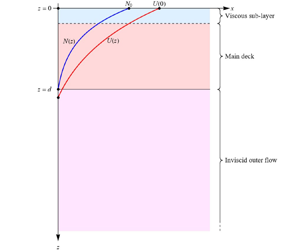
  $t^{\star }$. Both the shear and stratification are confined to the boundary layer as sketched in figure 1. There are no other assumptions regarding the profiles of the shear and stratification.

Figure 1. Sketch of geometry of a generic free-surface boundary-layer profile with the shear and stratification localized in a layer of thickness  $d$. The vertical scales of shear and stratification are assumed be of the same order as the boundary-layer thickness $d$. No other assumptions regarding the profiles of shear and stratification are required. A typical free-surface boundary layer has the maximum of velocity at the surface $U_{max}=U(0)$.
In the Cartesian frame with the fluid occupying the half-space  $z^{\star }>0$ and with $x^{\star }$ and $y^{\star }$ directed streamwise and spanwise, respectively, the Navier–Stokes equations complemented by the mass conservation and incompressibility equations take the form
 \begin{gather} \rho_{0}^{{\star}}[D_{t^{{\star}}}u^{{\star}}+w^{{\star}}U^{{\star}\prime}]+ p_{x^{{\star}}}^{{\star}} ={-}\bar{\rho}^{{\star}}[D_{t^{{\star}}}u^{{\star}}+ w^{{\star}}U^{{\star}\prime}] -\rho_{0}^{{\star}}(\boldsymbol{u}^{{\star}}\boldsymbol{\cdot}\boldsymbol{\nabla})u^{{\star}}- \bar{\rho}^{{\star}}(\boldsymbol{u}^{{\star}}\boldsymbol{\cdot}\boldsymbol{\nabla})u^{{\star}} \nonumber\\ +\,\mu^{{\star}}\nabla^{2}u^{{\star}}, \end{gather}
 $$\begin{gather} \rho_{0}^{{\star}} D_{t^{{\star}}}v^{{\star}}+p_{y^{{\star}}}^{{\star}}={-}\bar{\rho}^{{\star}} D_{t^{{\star}}}v^{{\star}}-\rho_{0}^{{\star}} (\boldsymbol{u}^{{\star}}\boldsymbol{\cdot}\boldsymbol{\nabla})v^{{\star}}-\bar{\rho}^{{\star}} (\boldsymbol{u}^{{\star}}\boldsymbol{\cdot}\boldsymbol{\nabla})v^{{\star}}+ \mu^{{\star}}\nabla^{2}v^{{\star}}, \end{gather}$$
 $$\begin{gather}\rho_{0}^{{\star}} D_{t^{{\star}}}w^{{\star}}+p_{z^{{\star}}}^{{\star}}+ \bar{\rho}^{{\star}}g^{{\star}}={-}\bar{\rho}^{{\star}} D_{t^{{\star}}}w^{{\star}}- \rho_{0}^{{\star}}(\boldsymbol{u}^{{\star}}\boldsymbol{\cdot}\boldsymbol{\nabla})w^{{\star}}- \bar{\rho}^{{\star}}(\boldsymbol{u}^{{\star}}\boldsymbol{\cdot}\boldsymbol{\nabla})w^{{\star}}+ \mu^{{\star}}\nabla^{2}w^{{\star}}, \end{gather}$$
 $$\begin{gather}D_{t^{{\star}}}\bar{\rho}^{{\star}}+w^{{\star}} {\rho_{0}^{{\star}}}^{\prime} =K^{{\star}}\nabla^{2}\bar{\rho}^{{\star}}- (\boldsymbol{u}^{{\star}}\boldsymbol{\nabla}) \bar{\rho}^{{\star}}, \end{gather}$$
 $$\begin{gather}\boldsymbol{\nabla}\boldsymbol{\cdot}\boldsymbol{u}^{{\star}}=0, \end{gather}$$
where  $\boldsymbol {U}^{\star }=(U^{\star }(z^{\star }),0,0)$ is the basic flow localized in the boundary layer, $\boldsymbol {u}^{\star }=(\boldsymbol {q}^{\star },w^{\star })=(u^{\star },v^{\star },w^{\star })$ and $p^{\star }$ are, respectively, the velocity and pressure perturbations, $D_{t^{\star }}=\partial _{t^{\star }}+U^{\star }\partial _{x^{\star }}$ is the material derivative, $\mu ^{\star }$ is the dynamic viscosity, while $K^{\star }$ is the mass diffusivity coefficient, $\nabla ^{2}$ stands for the 3-D Laplacian. Here, the prime denotes the derivatives with respect to $z^{\star }$. When the model is applied to turbulent boundary layers, viscosity and diffusivity are understood as eddy viscosity and diffusivity and, for simplicity, assumed to be constant. We impose no restrictions on $\boldsymbol {U}^{\star }(z^{\star })$, apart from the assumption that the flow is plane parallel (non-parallel effects and 3-D boundary layers will be considered elsewhere). In contrast to the original derivations in Shrira (Reference Shrira1989) and Voronovich et al. (Reference Voronovich, Shrira and Stepanyants1998), we do not require ${U}^{\star }(z^{\star })$ not to have inflection points.
The boundary conditions for the perturbations  $\boldsymbol {u}^{\star }$ at the undisturbed fluid surface $z^{\star }=0$ are: the ‘no-flux’ condition
 \begin{equation} w^{{\star}}(z^{{\star}}=0)=0, \end{equation}
complemented by the no-stress condition
 \begin{equation} \left.\frac{\partial u^{{\star}}}{\partial z^{{\star}}}\right|_{z^{{\star}}=0}= \left.\frac{\partial v^{{\star}}}{\partial z^{{\star}}}\right|_{z^{{\star}}=0}=0. \end{equation}
The boundary condition at infinity is that of vanishing perturbation velocity
 \begin{equation} \boldsymbol{u^{{\star}}} \to 0, \quad\mbox{as}\ z^{{\star}} \to \infty. \end{equation}
We complete the formulation of our initial problem by specifying the perturbation velocity field at the initial moment,  $\boldsymbol {u}^{\star }(\boldsymbol {x}^{\star }, 0)$. We are primarily interested in localized initial perturbations
 \begin{equation} \boldsymbol{u^{{\star}}}(\boldsymbol{x^{{\star}}}, 0)\to 0, \quad\mbox{as}\ x^{{\star}},y^{{\star}} \to \infty. \end{equation}
The Navier–Stokes equations (2.2) with the initial and boundary conditions (2.5), (2.3) and (2.4), constitute the mathematical formulation of the problem.
2.2. Scaling
We begin by specifying the scaling. The basic boundary-layer shear flow  $U^{\star }(z^{\star })$ has a maximal velocity, usually at the surface, which we denote as $V_{0}^{\star }$. As a characteristic value of the buoyancy frequency $N^{\star }(z^{\star })$ we take its value $N_{0}^{\star }$ at the surface. If $N^{\star }(z^{\star }=0)$ vanishes, any other reference point can be chosen. The characteristic streamwise and spanwise scales of perturbations we denote as $L^{\star }$, while for the vertical scale we choose the boundary-layer thickness $d^{\star }$. We are considering long perturbations with $L^{\star }\gg d^{\star }$. We non-dimensionalize the variables as follows:
 \begin{equation} \left.\begin{gathered} \tilde{u}=\frac{u^{{\star}}}{V_{0}^{{\star}}},\quad \tilde{v}=\frac{v^{{\star}}}{V_{0}^{{\star}}},\quad \tilde{w}=\frac{w^{{\star}}}{V_{0}^{{\star}}},\quad \tilde{x}=\frac{x^{{\star}}}{L^{{\star}}},\\ \tilde{y}=\frac{y^{{\star}}}{L^{{\star}}},\quad \tilde{z}=\frac{z^{{\star}}}{d^{{\star}}}, \quad \tilde{U}=\frac{U^{{\star}}}{V_{0}^{{\star}}},\quad \tilde{t}=\frac{V_{0}^{{\star}}}{L^{{\star}}}t^{{\star}},\\ \tilde{N}=\frac{N^{{\star}}}{N_{0}^{{\star}}},\quad \tilde{p}= \frac{p^{{\star}}}{\rho_{0}^{{\star}}{V_{0}^{{\star}}}^{2}},\quad \tilde{\rho}=\frac{\rho^{{\star}}}{\rho_{0}^{{\star}}}, \end{gathered}\right\} \end{equation}
where tildes denote non-dimensional quantities. To proceed, we first estimate the magnitudes of the perturbations from the governing equations (2.2). With tildes omitted the magnitude of the vertical velocity perturbation  $[\,w\,]$ expressed in terms of the magnitudes of the horizontal components $[\,q\,]$,
 \begin{equation} [\,w\,]=\frac{d^{{\star}}}{L^{{\star}}}[\,q\,]. \end{equation}
The momentum equation (2.2a) yields the characteristic time scale,
 \begin{equation} [\,t\,]=\frac{L^{{\star}}}{V_{0}^{{\star}}}. \end{equation}
On multiplying mass conservation equation (2.2d) by  $g^{\star }$ and dividing it by the reference density $\rho _{0}^{\star }$, we substitute buoyancy frequency $N^{\star 2}$ for $({g^{\star }}/{\rho _{0}^{\star }}) ({\partial \rho _{0}^{\star }}/{\partial z^{\star }})$ using the Boussinesq approximation, which yields
 \begin{equation} g^{{\star}}D_{t^{{\star}}}\left(\frac{\bar{\rho}^{{\star}}}{\rho_{0}^{{\star}}}\right) + w^{{\star}}N^{\star2}(z^{{\star}})=g^{{\star}}\frac{\nu^{{\star}}}{Sc\rho_{0}^{{\star}}} \nabla^{2}\bar{\rho}^{{\star}}-\frac{g^{{\star}}}{\rho_{0}^{{\star}}} (\boldsymbol{u}^{{\star}}\boldsymbol{\nabla})\bar{\rho}^{{\star}}, \end{equation}
where  $Sc=\nu ^{\star }/{K^{\star }}$ is the Schmidt number, the ratio of the kinematic viscosity $\nu ^{\star }={\mu ^{\star }}/ {\rho _{0}^{\star }}$ and mass diffusivity ${K^{\star }}$.
To proceed we express (2.10) in non-dimensional form and substitute equations (2.8) and (2.9), to get an estimate characteristic magnitude of density perturbations (tildes and star dropped)
 \begin{equation} \left[\frac{\bar{\rho}}{\rho_{0}}\right]=\frac{N_{0}^{2}d}{g}\frac{[\,q\,]}{V_{0}}. \end{equation}
In the derivation, we employ the Boussinesq approximation, whereby, if not multiplied by  $g$, we neglect the terms in the equations due to the equilibrium density $\rho _{0}$ variations. The Boussinesq approximation holds under the assumption
 \begin{equation} \frac{N_{0}^{2}}{g/d}\ll \frac{[\,q\,]}{V_{0}}, \end{equation}
which is valid in most oceanic and atmospheric contexts where the equilibrium density variations are small. This inequality allows us to drop small nonlinear buoyancy terms. In nature the parameters of the surface layer of the ocean vary very widely. Still, we provide a few characteristic values:  $V_0^{\star }\sim 10^{-1}$ m s $^{-1}$, $d^{\star } \sim 50\,\textrm {m},\ N_0 \sim 10^{-4}\,\textrm {s}^{-1}$.
The regimes we study are characterized by four independent non-dimensional small/large parameters specifying, respectively,
(i) the smallness of nonlinearity: ${[\,q^{\star }\,]}/{V_{0}^{\star }}=\varepsilon \ll 1$;
(ii) the smallness of characteristic wavenumbers, which we also refer to as the dispersion parameter:
${d^{\star }}/{L^{\star }}=\varepsilon _{D}\ll 1$;(iii) the weakness of the boundary-layer stratification characterized by the Richardson number:
$Ri=({N_{0}^{\star }d^{\star }}/{V_{0}^{\star }})^{2}\ll 1$;(iv) the weakness of dissipative effects:
$Re^{-1}= {\nu ^{\star }}/{V_{0}^{\star }d^{\star }}\ll 1$.


From now on we will be using only the non-dimensional tilde variables (2.7) omitting the tildes. Under the Boussinesq approximation upon non-dimensionalization the Navier–Stokes equations (2.2) take the form
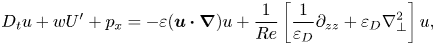 $$\begin{gather} D_{t}u+wU^{\prime}+p_{x}={-}\varepsilon(\boldsymbol{u}\boldsymbol{\cdot}\boldsymbol{\nabla})u+ \frac{1}{Re}\left[\frac{1}{\varepsilon_{D}}\partial_{zz}+ \varepsilon_{D}\nabla_{{\perp}}^{2}\right]u, \end{gather}$$
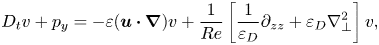 $$\begin{gather}D_{t}v+p_{y}={-}\varepsilon(\boldsymbol{u}\boldsymbol{\cdot}\boldsymbol{\nabla})v+ \frac{1}{Re}\left[\frac{1}{\varepsilon_{D}}\partial_{zz}+ \varepsilon_{D}\nabla_{{\perp}}^{2}\right]v, \end{gather}$$
 $$\begin{gather}D_{t}w+\frac{1}{\varepsilon_{D}}p_{z}+\varepsilon\varepsilon_{D}Ri \bar{\rho}={-}\varepsilon(\boldsymbol{u}\boldsymbol{\cdot}\boldsymbol{\nabla})w+ \frac{1}{Re}\left[\frac{1}{\varepsilon_{D}}\partial_{zz}+ \varepsilon_{D}\nabla_{{\perp}}^{2}\right]w, \end{gather}$$
 $$\begin{gather}D_{t}\bar{\rho}+ \frac{1}{\varepsilon_{D}}N^{2}(z)w=\frac{\varepsilon_{D}}{Re\, Sc}\left[\frac{1}{\varepsilon_{D}}\partial_{zz}+ \varepsilon_{D}\nabla_{{\perp}}^{2}\right]\bar{\rho}- \varepsilon(\boldsymbol{u}\boldsymbol{\nabla})\bar{\rho}, \end{gather}$$
 $$\begin{gather}\boldsymbol{\nabla}\boldsymbol{\cdot}\boldsymbol{u}=0, \end{gather}$$
where  $\nabla _{\perp }^{2}=\partial _{xx}^{2}+\partial _{yy}^{2}$.
After some algebra, upon eliminating pressure from (2.13), we get a single equation for the vertical component of velocity  ${w}$
${w}$
 \begin{equation} D_{t}^{2}\partial_{zz}^2w-U^{\prime\prime}D_{t}\partial_{x}w={\mathcal{N}} -Ri\,N^{2}\nabla_{{\perp}}^{2}w+\left(\varepsilon_{D}Re\right)^{{-}1}D_{t} \partial_{zzzz}^{4}w+{\mathcal{M}}, \end{equation}
where
 \begin{equation} \left.\begin{gathered} {\mathcal{N}}=\varepsilon D_{t}\partial_{z} \boldsymbol{\nabla}_{{\perp}}[(\boldsymbol{u}\boldsymbol{\nabla})\boldsymbol{q}]- \varepsilon_{D}^{2}D_{t}^{2}\nabla_{{\perp}}^{2}w-\varepsilon_{D}^{2} \varepsilon D_{t}\nabla_{{\perp}}^{2}(\boldsymbol{u}\boldsymbol{\nabla})w,\\ {\mathcal{M}}=Ri \varepsilon\nabla_{{\perp}}^{2}(\boldsymbol{u}\boldsymbol{\nabla})\bar{\rho}+ \frac{1}{Sc\,Re}Ri\varepsilon\nabla_{{\perp}}^{2}\bar{\rho}^{\prime\prime}. \end{gathered}\right\} \end{equation}
Note that the equation is closed only in the linear approximation and just the leading-order viscous and diffusion terms are retained. The contribution of diffusion of mass is characterized by the inverse Schmidt number. Under assumption  $Sc\sim O(1)$ diffusion of mass proves to be negligible in our further analysis.
Aiming to describe the dynamics of 3-D perturbations in the boundary layer taking into account nonlinearity, long-wave dispersion, stratification and viscous effects in the distinguished limit we set
 \begin{equation} \varepsilon=\frac{[\,q\,]}{V_{0}}\ll 1,\quad \varepsilon_{D}=\frac{d}{L}= O(\varepsilon),\quad Ri=\left(\frac{N_{0}d}{V_{0}}\right)^{2}=O(\varepsilon),\quad Re=O(\varepsilon^{{-}2}). \end{equation}
The adopted scaling can be also expressed in terms of the Reynolds number
 \begin{equation} \varepsilon \sim Re^{{-}1/2}, \quad \varepsilon_{D} \sim Re^{{-}1/2}, \quad Ri \sim Re^{{-}1/2}. \end{equation}
2.3. Asymptotic expansion
To rationalize our choice of asymptotic expansion in powers of  $\varepsilon$, it is helpful to consider first the inviscid non-stratified reduction of the Navier–Stokes equations (2.13) linearized around the steady profile $U(z)$ with pressure $p$, the streamwise and transverse perturbation velocities, $u$ and $v$, expressed in terms of vertical velocity $w$ (see e.g. Miropol'sky (Reference Miropol'Sky2001), (2.58)). For long-wave perturbations such a reduction reads
 $$\begin{gather} \partial_{z}D_{t}u={-}[\partial_{z}(wU^{\prime}) -\partial_{x}(D_{t}w)], \end{gather}$$
 $$\begin{gather}\partial_{z}D_{t}v=\partial_{y}(D_{t}w), \end{gather}$$
 $$\begin{gather}\partial_{z}p=D_{t}w . \end{gather}$$
Noting that, under adopted assumptions specifying the wavelength scale of the perturbations in terms of the nonlinearity parameter,  $\varepsilon _{D}= O(\varepsilon )$, we have
 \begin{equation} \partial_{x}\sim \partial_{y}\sim O(\varepsilon), \quad\partial_{z}\sim O(1). \end{equation}
Since in our scaling  $U,U^{\prime }\sim O(1)$, it is easy to see that to leading order the material derivative $D_{t}=(U-c)\partial _{x}\sim O(\varepsilon )$, where $c$ is an unspecified yet phase velocity of long perturbations. By virtue of our definition of $\varepsilon (\varepsilon =[u]/V_0)$, $u$ is $O(\varepsilon )$. Therefore, upon omitting the higher-order terms, the relations (2.18) reduce to
 $$\begin{gather} (U-c)\partial_{x} u={-}\underbrace{wU^{\prime}}_{O(\varepsilon^{2})},\quad \implies w\sim O(\varepsilon^{2}), \end{gather}$$
 $$\begin{gather}\partial_{z}[(U-c)v]=\underbrace{\partial_{y}(U-c)w}_{O(\varepsilon^{3})}, \quad\implies v\sim O(\varepsilon^{3}), \end{gather}$$
 $$\begin{gather}\partial_{z}p=\underbrace{(U-c) \partial_{x}w}_{O(\varepsilon^{3})},\quad \implies p \sim O(\varepsilon^{3}). \end{gather}$$
In addition to the above perturbation velocities scaling, we derive below the scaling of density from the linearized inviscid reduction of the Navier–Stokes equation. First, it is straightforward to express perturbation density  $\bar {\rho }$ in terms of vertical velocity $w$ from the linearized equation (2.10) according to
 \begin{equation} gD_{t}\left(\frac{\bar{\rho}}{\rho_{0}}\right)=N^{2}w,\quad \implies g(U-c)\partial_{x}\bar{\rho}=\underbrace{\rho_{0}}_{O(1)} \underbrace{N^{2}w}_{O(\varepsilon^{3})},\quad \bar{\rho}\sim O(\varepsilon^{2}). \end{equation}
Thus, assuming the streamwise perturbation velocity  $u$ to be $O(\varepsilon )$ and setting $\varepsilon _{D}={d}/{L} = O(\varepsilon )$ uniquely dictates the scaling (2.20), (2.10) of all other dependent variables inside the boundary layer. Taking into account the nonlinear and viscous terms neglected in this analysis does not affect the found scaling. We note that the above scaling has no self-consistent alternatives. Therefore, for the full Navier–Stokes equations (2.13) in the boundary layer we adopt the following asymptotic expansion:
 $$\begin{gather} u=U(z)+\varepsilon u_{1}+\varepsilon^{2}u_{2}+\varepsilon^{3}u_{3}+\cdots, \end{gather}$$
 $$\begin{gather}w=\varepsilon^{2}w_{2}+\varepsilon^{3}w_{3}+\varepsilon^{4}w_{4}+\cdots, \end{gather}$$
 $$\begin{gather}v=\varepsilon^{3}v_{3}+\varepsilon^{4}v_{4}+\cdots, \end{gather}$$
 $$\begin{gather}p=\varepsilon^{3}p_{3}+\varepsilon^{4}p_{4}+\cdots, \end{gather}$$
 $$\begin{gather}\bar{\rho}=\varepsilon^{2}\bar{\rho}_{2}+\varepsilon^{3}\bar{\rho}_{3}+\cdots, \end{gather}$$
where  $u_i, v_i, w_i, p_i$ and $\bar {\rho }_{i}$ are $O(1)$ functions of $x,y,z, t$. The scaling (2.22) will be employed only inside the boundary layer, while outside the boundary layer and in the immediate vicinity of the boundary, in the viscous sub-layer, the scaling is different and will be specified in the next section.
3. Derivation of the nonlinear evolution equation
3.1. Preliminary consideration. Layout of the triple-deck scheme
In this section we derive the nonlinear evolution equation (1.1) for long-wave 3-D perturbations employing a version of the ‘triple deck’ asymptotic approach (e.g. Neiland Reference Neiland1969; Stewartson Reference Stewartson1969; Messiter Reference Messiter1970; Van Dyke Reference Van Dyke1975). As is common for this approach, we distinguish three domains or ‘decks’ in  $z$, with different balance between the terms in (2.14). The domains are sketched in figure 2. Following the convention the bulk of the boundary layer is referred to as the ‘main deck’ or ‘middle deck’. There we balance nonlinearity, dispersion and viscous effects and employ the asymptotic expansion (2.22). Immediately adjacent to the boundary lies much thinner viscous sub-layer or the ‘first deck’, where viscous terms are dominant, while the nonlinearity is small, but not negligible. The semi-infinite domain outside the boundary layer, where both viscous and nonlinear terms are negligible and the flow is potential, is referred to as the ‘outer flow’ or the ‘third deck’. We adopt this terminology introduced by Stewartson (Reference Stewartson1969). In contrast to the widely followed convention we do not a priori scale our variables in terms of powers of inverse Reynolds number, in our context we prefer to use the scaling in powers of $\varepsilon$. The derivation largely follows that in Voronovich et al. (Reference Voronovich, Shrira and Stepanyants1998), with three key differences:
(i) In contrast to Voronovich et al. (Reference Voronovich, Shrira and Stepanyants1998), the presence of weak stratification in the boundary layer (‘main deck’) is taken into account; we consider stratification to be weak and localized inside the boundary layer.
(ii) The Reynolds number here is allowed to be smaller:
$Re\sim \varepsilon ^{-2}$, not $\sim \varepsilon ^{-3}$.(iii) No assumption regarding the absence of inflection points is required.
Figure 2. Sketch of triple-deck structure illustrating three different regions. The first region adjacent to the boundary is the viscous sub-layer where viscosity dominates, the middle region is the main deck, where nonlinearity, dispersion, stratification and viscosity are all balanced. The third semi-infinite region is the outer flow region where the motion is irrotational.
The rationale for the assumption (iii) was to exclude a priori the possibility of linear inflectional instability, which, in principle, might interfere with the nonlinear dynamics we are studying. However, a closer look at the now available results on linear instabilities in boundary layers (e.g. Healey Reference Healey2017) enabled us to lift the restriction. Although the profiles with inflection points can be indeed unstable, these inflectional instabilities are long-wave instabilities with the maximal growth rates
$O(\varepsilon ^{3})$ and, thus, do not affect the processes with the $O(\varepsilon ^{-2})$ characteristic periods which we focus upon.


3.2. Inside the boundary layer. The main deck
We begin with analysis of the motion in the main deck. The scaling (2.22) based upon the distinguished limit which balances nonlinearity, weak dispersion, stratification and viscosity, provides the basis of our asymptotic analysis inside the main deck. On substituting the already adopted relations between the small parameters:  $\varepsilon _{D} \sim Ri\sim \varepsilon$, and introducing re-scaled Richardson and Reynolds numbers denoted as $Ri_{\ast }$ and $Re_{\ast }$, such that $Ri=\varepsilon Ri_{\ast }$ and $Re_{\ast }=\varepsilon ^{2} Re$, into equation (2.14), we make the scaling of each term more explicit
 \begin{equation} D_{t}^{2}\partial_{zz}^2 w-U^{\prime\prime}D_{t}\partial_{x}w= \varepsilon D_{t}\partial_{z}{\mathcal{N}}_{L}-\varepsilon Ri_{{\ast}} N^{2}\nabla_{{\perp}}^{2}w +\frac{\varepsilon}{Re_{{\ast}}}D_{t}w^{iv}-\varepsilon^{2}D_{t}^{2}\nabla_{{\perp}}^{2}w+{\mathcal{M}}_{1}, \end{equation}
where
 \begin{equation} {\mathcal{M}}_{1}=\varepsilon^{2}Ri_{{\ast}}\nabla_{{\perp}}^{2} (\boldsymbol{u}\boldsymbol{\nabla})\bar{\rho}-\varepsilon^{3} D_{t}\nabla_{{\perp}}^{2}(\boldsymbol{u}\boldsymbol{\nabla})w+ \varepsilon^{4}\frac{1}{Sc\,Re_{{\ast}}}Ri_{{\ast}}\nabla_{{\perp}}^{2}\bar{\rho}^{\prime\prime}, \end{equation}
and
 \begin{align} {\mathcal{N}}_{L} &= [\partial_{x}(u\partial_{x}u+v\partial_{y}u+w\partial_{z}u)+ \partial_{y}(u\partial_{x}v+v\partial_{y}v+w\partial_{z}v)], \nonumber\\ &=[\varepsilon\partial_{x}(\varepsilon^{3}u\partial_{x}u+ \varepsilon^{5}v\partial_{y}u+\varepsilon^{3}w\partial_{z}u)+ \varepsilon\partial_{y}(\varepsilon^{5}u\partial_{x}v+ \varepsilon^{7}v\partial_{y}v+\varepsilon^{5}w\partial_{z}v)] \nonumber\\ &=\varepsilon^{4}[\partial_{x}(u\partial_{x}u+w\partial_{z}u)] + \varepsilon^{6}[\partial_{x}(v\partial_{y}u) +\partial_{y} (u\partial_{x}v +w\partial_{z}v +\varepsilon^{2} v\partial_{y}v)]. \end{align}
Although the streamwise and spanwise scales are assumed to be comparable, according to (2.22) the spanwise velocity is two orders of magnitude smaller, which enables us to split the nonlinear term  ${\mathcal {N}}_{L}$ into three parts and neglect the $O(\varepsilon ^{6})$, $O(\varepsilon ^{7})$ and $O(\varepsilon ^{8})$ contributions. The terms $\varepsilon ^{2}Ri_{\ast }\nabla _{\perp }^{2}(\boldsymbol {u}\boldsymbol {\nabla })\bar {\rho }$, $\varepsilon ^{4}({1}/{Sc\,Re_{\ast }})Ri_{\ast }\nabla _{\perp }^{2}\bar {\rho }^{\prime \prime }$ and $\varepsilon ^{3} D_{t}\nabla _{\perp }^{2}((\boldsymbol {u}\boldsymbol {\nabla })w)$, on the right-hand side of (3.1) are $O(\varepsilon ^{7})$ and above, these terms will also be neglected in our further analysis. Upon these simplifications, recalling that $w=O(\varepsilon ^{2})$, we re-write (3.1) explicitly pulling out $\varepsilon$
 \begin{align} \underbrace{D_{t}^{2}\partial_{zz}^2w-U^{\prime\prime}D_{t} \partial_{x}w}_{O(\varepsilon^{4}{terms})} &= \varepsilon^{5}D_{t}\partial_{z}\partial_{x} [u\partial_{x}u+w\partial_{z}u]-\varepsilon^{5}Ri_{{\ast}}N^{2}\nabla_{{\perp}}^{2}w+\cdots \nonumber\\ &\quad +\frac{\varepsilon^{5}}{Re_{{\ast}}}D_{t}w^{iv}- \varepsilon^{6}D_{t}^{2}\nabla_{{\perp}}^{2}w. \end{align}
Since  $v= O(\varepsilon ^{3})\ \mbox {and}\ u=O(\varepsilon ^{1})$, it is easy to see that, by virtue of the continuity equation, $\partial _{x}u= -\partial _{z}w + O(\varepsilon ^{4})$. To solve (3.4) we adopt a moving coordinate frame $x\to x-ct$ and use standard multiple-scale method by introducing fast and slow non-dimensional independent variables
 \begin{equation} Z_{1}=\varepsilon z,\quad \tau=\varepsilon t, \end{equation}
where we recall that  $c$ is the speed of perturbations in the long-wave limit which will be specified later. Then the squared material derivative $D_{t}^{2}$ and $\partial _{zz}^{2}$ take the form
 \begin{equation} D_{t}^{2}=\frac{V_{0}^{2}}{L^{2}}[(U-c)\partial_{x}+\varepsilon\partial_{\tau}]^{2}= \frac{V_{0}^{2}}{L^{2}}D_{t}^{2}\sim\varepsilon^{2}D_{t}^{2},\quad \partial_{zz}^{2}=\frac{1}{d^{2}}(\partial_{z}+\varepsilon\partial_{Z_{1}})^{2}\approx \frac{1}{d^{2}}\partial_{zz}^{2}\sim\partial_{zz}^{2}. \end{equation}
Equation (3.4) for the vertical component of velocity,  $w$, reduces to
 \begin{equation} D_{t}^{2}\partial_{zz}^2w-U^{\prime\prime}D_{t}\partial_{x}w=\varepsilon D_{t}\partial_{z}\partial_{x} [u\partial_{x}u+w\partial_{z}u]-\varepsilon Ri_{{\ast}} N^{2}\nabla_{{\perp}}^{2}w+\frac{\varepsilon}{Re_{{\ast}}} D_{t}w^{\prime\prime\prime\prime}-\varepsilon^{2}D_{t}^{2}\nabla_{{\perp}}^{2}w, \end{equation}
where
 \begin{equation} D_{t}=(U-c)\partial_{x}+\varepsilon\partial_{\tau},\quad \partial_{z}=\partial_{z}+\varepsilon\partial_{Z_{1}}. \end{equation}
We recall that the mean flow  $U(z)$ and stratification $N(z)$ are assumed to be localized in the boundary layer and, correspondingly, to depend only on the fast scale $z$.
$z$.
First, we impose the no-flux condition at  $z=0$. We will deal with the complete boundary conditions at the boundary in § 3.4. We also require vanishing of the velocity as $Z_{1}\to \infty$. In addition, we introduce ‘inner boundary conditions’, the condition of matching at the outer boundary of the boundary layer. Thus,
 \begin{equation} w(z=0)=0;\quad w(z\to \infty)=const=w(Z_{1}\to 0),\quad w({Z_{1}\to \infty})\to 0. \end{equation}
We will seek an asymptotic solution to the boundary value problem (3.7), (3.8a,b) and (3.8a,b) employing power series in  $\varepsilon$ (2.22). On finding the solution to (3.7) for $w$ at a certain order in $\varepsilon$, we find $u,v$ and $p$ with the corresponding accuracy from the basic equations
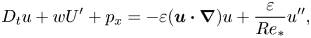 $$\begin{gather} D_{t}u+wU^{\prime}+p_{x}={-}\varepsilon(\boldsymbol{u}\boldsymbol{\cdot}\boldsymbol{\nabla})u+ \frac{\varepsilon}{Re_{{\ast}}}u^{\prime\prime}, \end{gather}$$
 $$\begin{gather}D_{t}v+p_{y}={-}\varepsilon(\boldsymbol{u}\boldsymbol{\cdot}\boldsymbol{\nabla})v+ \frac{\varepsilon}{Re_{{\ast}}}v^{\prime\prime}, \end{gather}$$
 $$\begin{gather}\partial_{x}u+\partial_{y}v+\partial_{z}w=0. \end{gather}$$
The solutions for  $u$,
$u$,  $v$ and $p$, accurate to a corresponding order in $\varepsilon$, are further used for the derivation of the next order terms for $w$, the cycle is repeated as many times as necessary.
At the first step, on substituting (2.22) into (3.7) and setting  $\varepsilon =0$, we see that in the leading-order nonlinearity, stratification and viscous dissipation drop out. Taking into account (3.8a,b) we obtain for $w_{2}$ the long-wave limit of the Rayleigh equation
 \begin{equation} (U-c)\partial_{xx}[(U-c)w_{2}^{\prime\prime}-U^{\prime\prime}w_{2}]=0, \end{equation}
where derivatives with respect to the fast variable  $z$ are denoted by primes. It can be easily seen from (3.11) that the $x,y$ and $z$ dependencies can be separated. Assuming the disturbance to be localized or periodic in the streamwise direction, the general solution to equation (3.11) is convenient to present in the form
 \begin{equation} w_{2}=[f(x,y,Z_{1})\ast\partial_{x}A(x,y,\tau)]\cdot(U(z)-c), \end{equation}
where  $\ast$ designates the convolution of two functions
 \begin{equation} \varphi\ast\psi=\int_{-\infty}^{+\infty}\int_{-\infty}^{+\infty}\varphi({x}^{\prime},{y}^{\prime}) \psi(x-{x}^{\prime},y-{y}^{\prime})\,\mathrm{d}{x}^{\prime}\,\mathrm{d}{y}^{\prime}. \end{equation}
Here, as will be made explicit a few lines below,  $A(x,y,\tau )$ is the amplitude of the $x$-component of velocity perturbation, while the arbitrary function $f(x,y,Z_{1})$ in (3.12) is the general representation of a function of $(x,y,Z_{1},\tau )$ localized or periodic in $(x,y)$. The fundamental properties of the presentation (3.12) become more transparent on performing the Fourier transform of ansatz (3.12). The standard way of representing a function of $(x,y,Z_{1},\tau )$ is to decompose it into a set of spatial orthogonal functions with time-dependent amplitudes. We chose Fourier in $(x,y)$ and a particular function $f$ specifying each Fourier mode that depends on the slow vertical spatial variable $Z_{1}$. The specific dependence on the slow spatial scale $f(Z_{1})$ will be found a few lines below. The boundary condition $w_{2}(z=0)=0$ specifies the eigenvalue $c$
$c$
 \begin{equation} c=U|_{z=0}\equiv U_0. \end{equation}
The mode we are considering is to leading order a vorticity wave, modified in the next orders by stratification and viscosity. To leading order its speed is the mean flow velocity at  $z=0$, which usually is its maximal value for the typical ‘no-stress’ flows. In any case, it plays no role in our further analysis since its only significance is in specifying the reference frame, the surface velocity $U_0$ will be removed by the Galilean transformation at the next step.
To proceed further, we first find the other components of perturbation wave field from (3.10) using the asymptotic expansion (2.22). On substituting the leading-order solution for  $w_{2}$ into (3.10) we find the other components of the perturbation field
 $$\begin{gather} u_{1}={-}U^{\prime}(f\ast A), \end{gather}$$
 $$\begin{gather}v_{2}=0, \end{gather}$$
 $$\begin{gather}p_{2}=0. \end{gather}$$
Note that (3.15a) clarifies the physical sense of amplitude  $A$, it is indeed, up to a factor $-U^{\prime }$, the amplitude of the $x$-component of perturbation velocity. The above relations show that to leading order the motion is extremely simple: the particles of the vorticity wave motion just oscillate in the streamwise direction, while the vertical and, especially, spanwise velocities and pressure perturbations are much smaller in the adopted long-wave approximation. This peculiar feature is specific for long vorticity waves (see Voronovich et al. Reference Voronovich, Shrira and Stepanyants1998). Such a simplicity of the motion of interest in the leading order is the key element enabling for a remarkably simple description of the 2-D nonlinear dynamics of vorticity waves which we will discuss below.
Substituting expressions (3.12) for  $w_{2}$ and (3.15a) for $u_1$ into (3.7) we get an equation for $w_{3}$
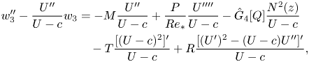 \begin{align} w_{3}^{\prime\prime}-\frac{U^{\prime\prime}}{U-c}w_{3} &={-}M\frac{U^{\prime\prime}}{U-c}+\frac{P}{Re_{{\ast}}} \frac{U^{\prime\prime\prime\prime}}{U-c}-\hat{G}_{4}[Q]\frac{N^{2}(z)}{U-c} \nonumber\\ &\quad -T\frac{[(U-c)^{2}]^{\prime}}{U-c}+R \frac{[(U^{\prime})^{2}-(U-c)U^{\prime\prime}]^{\prime}}{U-c}, \end{align}
where
 \begin{gather}
\begin{gathered}
M=(f\ast A_{\tau}),\quad
P=(f\ast A),\quad Q=(f\ast A_{x}),\quad T=(f_{Z_{1}}\ast A_{x}),\nonumber\\
R=(f\ast A)(f\ast A_{x}),
\end{gathered}
\end{gather}
\begin{gather}
\begin{gathered}
M=(f\ast A_{\tau}),\quad
P=(f\ast A),\quad Q=(f\ast A_{x}),\quad T=(f_{Z_{1}}\ast A_{x}),\nonumber\\
R=(f\ast A)(f\ast A_{x}),
\end{gathered}
\end{gather}
and  $\hat {G}_{4}$ is an integral operator which in the Fourier space is equivalent to multiplication by ${(k_{x}^{2}+k_{y}^{2})}/{k_{x}^{2}}$. The subscripts $x$,
$x$, $\tau$ and $Z_{1}$ stand for the corresponding partial derivatives. Recall that the buoyancy frequency $N(z)$ is confined to the boundary layer, i.e.
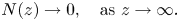 \begin{equation} N(z)\rightarrow 0, \quad\mbox{as}\ z\rightarrow\infty . \end{equation}
At the boundary  $N(z=0)=N_{0}$. Usually, $N_{0}$ is the maximum of $N(z)$, but this point is immaterial for our consideration. The general solution to the inhomogeneous Rayleigh equation (3.16) can be written as
 \begin{align} w_{3} &= M-T(U-c)\int^{\infty}_{z}\mathrm{d}\xi+B(U-c)\int^{\infty}_{z} \frac{\mathrm{d}\xi}{(U-c)^{2}} \nonumber\\ &\quad +\frac{P}{Re_{{\ast}}}(U-c)\int^{\infty}_{z} \left[\frac{U^{\prime\prime\prime}}{(U-c)^{2}}\right]\mathrm{d}\xi- \hat{G}_{4}[Q](U-c)\int_{z}^{\infty}\left[\frac{S(\xi)}{(U-c)^{2}}\right]\mathrm{d}\xi-RU^{\prime}. \end{align}
The contribution of stratification is given by the term with  $\hat {G}_{4}[Q]$, where function $S(z)$ in the integrand is proportional to the difference of the local reference density and that of the homogeneous fluid; it is given by the integral
 \begin{equation} S(z)=\int_{z}^{\infty}N^{2}(\xi)\,\mathrm{d}\xi. \end{equation}
In (3.19)  $B$ is an arbitrary constant specifying the ‘amplitude’ of the diverging fundamental solution to the homogeneous Rayleigh equation in the long-wave limit. To eliminate singularity in the integrals in (3.19) we chose $B$ in such a way that the equation for $w_{3}$ takes the form
 \begin{align} w_{3} &= M-T(U-c)\int_{z}^{\infty}[1-Y(U-c)^{{-}2}]\,\mathrm{d}\xi+ \frac{P}{Re_{{\ast}}}(U-c)\int_{z}^{\infty} \left[\frac{U^{\prime\prime\prime}}{(U-c)^{2}}\right]\mathrm{d}\xi \nonumber\\ &\quad -\hat{G}_{4}[Q](U-c)\int_{z}^{\infty} \left[\frac{S(z)}{(U-c)^{2}}\right]\mathrm{d}\xi-RU^{\prime} , \end{align}
where the integration constant  $Y$ has been chosen to be
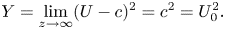 \begin{equation} Y=\lim_{z\rightarrow\infty}(U-c)^{2}=c^{2}=U_{0}^{2}. \end{equation}
 To evaluate the singular integrals above in (3.21) we assume that  $U^{\prime \prime \prime }(0)\ne 0$ and $U^{\prime }(0)\ne 0$ and expand $U-c$ near the boundary as $U^{\prime }(0)z=U_0^{\prime }z$.
The derived main-deck solution (3.21) ought to be matched with the lower-deck solution, the matching is carried out in Appendix A. Here, we just note that, upon formally applying to solution (3.21), the no-flux condition at the boundary, i.e. requiring  $w|_{z=0,Z_{1}=0}=0$ we get, after some algebra, a closed equation for the amplitude $A$ containing so far unspecified function $f(Z_{1})$ of the slow vertical variable $Z_{1}$
 \begin{align} & (f(0)\ast A_{\tau})-U^{\prime}(0)\left(\left(f(0)\ast A\right) \left(f(0)\ast A_{x}\right)\right)+\left(\frac{U_{0}^{2}}{U^{\prime}(0)}\right) \left(f_{Z_{1}}(0)\ast A_{x}\right) \nonumber\\ &\quad -\frac{1}{2}U_{0}Ri\hat{G}_{2}[f(0)\ast A_{x}]+ \frac{1}{Re_{{\ast}}}\left(\frac{U^{\prime\prime\prime}(0)}{U^{\prime}(0)}\right) \left(f(0)\ast A\right)=0 , \end{align}
where  $f(0)\equiv f(x,y,Z_{1}=0)$. The a posteriori justification of our use of the no-flux boundary condition is provided in Appendix A. Of course, the small $z$ expansion becomes invalid in the immediate vicinity of the boundary, a composite uniformly valid expansion is derived in Appendix A. Operator $\hat {G}_{2}$, which appears in (3.23), is related to $\hat {G}_{4}$ as follows: in the Fourier space $\hat {G}_{2}$ and $\hat {G}_{4}$ correspond, respectively, to $k_y^2/k_x^2$ and $(k_y^2 +k_x^2)/k_x^2$. Going from (3.21) to (3.23) we have subtracted 1 from the kernel in $\hat {G}_{4}$ to get $\hat {G}_{2}$, which means that the small correction to the long-wave velocity caused by stratification $c_{1}=-\frac {1}{2}U_{0}Ri$ was taken into account by adjusting the speed of the moving coordinate frame, the adjustment eliminates the term $c_{1}A_{x}$ appearing in the old frame due to correction to the long-wave velocity.
3.3. Matching the outer flow
In this subsection in order to obtain our final evolution equation for the 3-D perturbation amplitude  $A$ we proceed to find the unknown function $f(Z_1)$ for the outer flow slow vertical motion and then substitute it into (3.23). To find the as yet unspecified dependence of the found solution (3.12) and (3.21) on the slow vertical variable $Z_{1}$, we first proceed to the next order in $\varepsilon$ in equation (3.7) for $w_{2}$. Following the same asymptotic procedure and using (3.12) and (3.21) we express $u, v, p$ in terms of amplitude $A$
$A$
 \begin{align} u_{2} &={-}Y(f_{Z_{1}}\ast \nabla_{{\perp}}^{{-}2}A_{xx}) (U-c)^{{-}1}+(f_{Z_{1}}\ast A)U^{\prime}\int_{z}^{\infty} \left[1-Y(U-c)^{{-}2}\right]\mathrm{d}\xi \nonumber\\ &\quad +\frac{1}{2}(f\ast A)^{2}U^{\prime\prime}+\hat{G}_{4}[P] \frac{S(z)}{U-c}+\hat{G}_{4}[P]U^{\prime}\int_{z}^{\infty} \left(\frac{S(z)}{(U-c)^{2}}\right)\mathrm{d}\xi \nonumber\\ &\quad -\frac{\hat{P}U^{\prime}}{Re_{{\ast}}}\int_{z}^{\infty} \left(\frac{U^{\prime\prime\prime}}{(U-c)^{2}}\right)\mathrm{d}\xi -\frac{\hat{P}}{Re_{{\ast}}}\frac{U^{\prime\prime\prime}}{(U-c)}, \end{align}
 $$\begin{align} v_{3}&={-}Y(f_{Z_{1}}\ast \nabla_{{\perp}}^{{-}2}A_{xy})(U-c)^{{-}1}+\hat{G}_{3}[(f\ast A)]S(z)(U-c)^{{-}1}, \end{align}$$
 $$\begin{align}p_{3}&=Y(f_{Z_{1}}\ast \nabla_{{\perp}}^{{-}2}A_{xx})-\hat{G}_{4}[(f\ast A)]S(z), \end{align}$$
where  $\hat {G}_{3}$ is a pseudo-differential operator specified below, while $\hat {P}=(f\ast \partial _{x}^{-1}A)$. In the Fourier space the $\textbf{r}$-space operators $\hat {G}_{3}$ correspond to $({k_{y}^{2}}/{k_{x}^{2}}) ({k^{2}}/{k_{x}^{2}})$. Further on we will use symbol $\Leftrightarrow$ to denote such correspondence. Expressions for $P$,
$P$,  $Y$ and $S(z)$ are given by (3.17a–e), (3.22) and (3.20).
Now consider the next-order term for the vertical velocity,  $w_{4}$. After some algebra it can be brought to the form
 \begin{align} \partial_{x}[(U-c)w_{4}^{\prime\prime}-U^{\prime\prime}w_{4}] &={-}(f_{Z_{1}Z_{1}}\ast A_{xx})(U-c)^{2} \nonumber\\ &\quad -(f\ast\nabla_{{\perp}}^{2}A_{xx})(U-c)^{2}+F(x,y,\tau,z,Z_{1}), \end{align}
where  $F(x,y,\tau,z,Z_{1})$, being specified by a very bulky expression, is not given here. Crucially, it tends to zero as $z\to \infty$ faster than $|z|^{-1}$. In contrast, for an arbitrary function of $f(x,y,Z_{1})$ the first two terms on the right-hand side of equation (3.27) do not tend to zero as $z\to \infty$. As a result, the integration of (3.27) yields secular growth of the correction $w_{4}$ as $z\to \infty$, which does not allow the matching condition $w(z\to \infty,Z_{1})\to \mbox {const}$ to be satisfied. We put these secular terms to zero, which gives us an equation determining the dependence of function $f$ on the slow variable $Z_{1}$
 \begin{equation} (f_{Z_{1}Z_{1}}\ast A_{xx})+(f\ast\nabla_{{\perp}}^{2}A_{xx})=0. \end{equation}
The equation is complemented by the boundary condition at infinity
 \begin{equation} w(Z_{1}\to\infty) =0. \end{equation}
To find  $f(Z_{1})$ we, exploiting the homogeneity of the problem with respect to horizontal coordinates, perform the Fourier transform with respect to $x,y$ in the boundary problem (3.28) and (3.29). Making the Fourier transform of the convolution and pulling out the terms with amplitude $A$, we get the boundary value problem
 \begin{equation} \partial_{Z_{1}Z_{1}}^{2}\hat{f}({\boldsymbol k})-k^{2}\hat{f}({\boldsymbol k})=0, \end{equation}
with the boundary conditions
 \begin{equation} \hat{f}({\boldsymbol k})|_{Z_{1} \to \infty}=0,\quad \hat{f}({\boldsymbol k})|_{Z_{1}=0}=1. \end{equation}
Here,  $\hat {f}({\boldsymbol k},Z_{1})$ is the Fourier transform of $f(x,y,Z_{1})$
 \begin{equation} f(x,y,Z_{1})=\frac{1}{4{\rm \pi}^{2}}\int_{-\infty}^{+\infty} \int_{-\infty}^{+\infty}\hat{f}(k_{x},k_{y},Z_{1}) \exp({{\rm i}(k_{x}x+k_{y}y)})\,\mathrm{d}k_{x}\,\mathrm{d}k_{y}, \end{equation}
and  $k=|\boldsymbol k|$, $k^{2}=k_{x}^{2}+k_{y}^{2}$. The simplest normalization, $\hat {f}({\boldsymbol k})|_{Z_{1}=0}=1$, has been introduced for convenience to normalize the motion in the outer deck $\hat {f}(k_{x},k_{y},Z_{1})$ near the boundary. As one could easily anticipate, the motion in the outer layer is potential and satisfies the Laplace equation (3.30). Hence, it is easy to find the solution of the boundary value problem (3.30), (3.31a,b) satisfying the boundary condition (3.31a,b)
 \begin{equation} \hat{f}(\boldsymbol{k}, Z_{1})=\exp({-kZ_{1}})\quad Z_{1}\to \infty. \end{equation}
Next, we designate  $\partial _{Z_{1}}\hat {f}(\boldsymbol {k},0)\equiv \check {F}(k_{x},k_{y})$ and take into account that, at the boundary, ${f}(0)=\delta (x)\delta (y)$. The solution to (3.30) readily yields the kernel of the integral operator $\check {F}(k)=-k$. Substituting these findings into (3.23), we obtain the nonlinear evolution equation for the amplitude of 3-D long-wave perturbations in the distinguished limit
 \begin{equation} A_{\tau}-\alpha_{n} AA_{x}-\beta_{1}\hat{G}_{1}[A_{x}]- \beta_{2}\hat{G}_{2}[A_{x}]+\gamma A=0, \end{equation}
where the non-local operators  $\hat {G}_{1}$ and $\hat {G}_{2}$ are
 $$\begin{gather} \hat{G}_{1}[\varphi(\boldsymbol{r})]=\frac{1}{4{\rm \pi}^{2}}\int_{-\infty}^{+\infty} \int_{-\infty}^{+\infty}|\boldsymbol{k}|\varphi(\boldsymbol{r}_{1}) \exp({{\rm i}\boldsymbol{k}(\boldsymbol{r}-\boldsymbol{r}_{1})})\,\mathrm{d}\boldsymbol{k}\,\mathrm{d}\boldsymbol{r}_{1}, \end{gather}$$
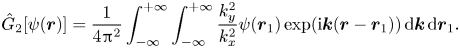 $$\begin{gather}\hat{G}_{2}[\psi(\boldsymbol{r})]=\frac{1}{4{\rm \pi}^{2}} \int_{-\infty}^{+\infty}\int_{-\infty}^{+\infty} \frac{k_y^{2}}{k_{x}^{2}}\psi(\boldsymbol{r}_{1})\exp({{\rm i}\boldsymbol{k} (\boldsymbol{r}-\boldsymbol{r}_{1})})\,\mathrm{d}\boldsymbol{k}\,\mathrm{d}\boldsymbol{r}_{1}. \end{gather}$$
Recall that  $k=|\boldsymbol {k}|=\sqrt {k_{x}^{2}+k_{y}^{2}}$. The coefficients are specified by the parameters of the flow at the surface: $\alpha _{n}=U^{\prime }(0), \beta _{1}={U_{0}^{2}}/{U^{\prime }(0)}, \gamma =({1}/{Re_{\ast }}){U^{\prime \prime \prime }(0)}/{U^{\prime }(0)}, \beta _{2}=U_0Ri/2$. The explicit account of viscous dissipation and weak stratification yield, respectively, the Rayleigh friction-type term $\gamma A$ and a very specific dispersion term $\beta _{2}\hat {G}_{2}[A_{x}]$ due to buoyancy. Coefficients $\alpha _{n}$ and $\beta _{1}$ of (3.34) can be removed by re-scaling to obtain the ‘universal’ form of the evolution equation. The equation is universal in the sense that the specific profiles of the boundary layer and stratification are immaterial. The residual specificity of the boundary layer retained in the coefficients $\alpha _{n}, \beta _{1}, \gamma, \beta _{2}$ in (3.34) can be further reduced by re-scaling the variables
 \begin{equation} \tau_{1}=\tau U^{\prime}(0),\quad d=\frac{U_{0}}{U^{\prime}(0)},\quad x_{1}=x/d,\quad A_{1}={-}\frac{1}{d}A, \end{equation}
which upon setting  $d=1$ and dropping the subscripts yields the ultimate form of the equation
 \begin{equation} A_{\tau}+AA_{x}-\hat{G}_{1}[A_{x}]-\tilde{\beta}_{2}\hat{G}_{2}[A_{x}]+\tilde{\gamma}A=0. \end{equation}
The non-local operators  $\hat {G}_{1}$ and $\hat {G}_{2}$ remain the same and are given by (3.35) and (3.36). The only remaining two coefficients
 \begin{equation} \tilde{\beta}_{2}=\frac{N_{0}^{2}}{2\varepsilon^2(U^{\prime}(0))^{2}},\quad \tilde{\gamma}= \frac{1}{Re_{{\ast}}} \frac{U^{\prime\prime\prime}(0)}{(U^{\prime}(0))^{2}},\quad Re_{{\ast}}=\varepsilon^{2}Re, \end{equation}
characterize the relative importance of the novel dispersion due to weak stratification and the Rayleigh friction-type term compared with the nonlinear one in the evolution equation. In this context the very weak  ${Ri}=O(\varepsilon )$ stratification proves to be essential. Although the flows with ${Ri}<1/4$ might be linearly unstable, in our context linear instabilities play no role since we focus on linearly stable situations; linear instabilities will be considered elsewhere.
3.4. Viscous sub-layer
3.4.1. Divergence of the asymptotic expansion and Tollmien's rescaling
Consider more closely behaviour of the main-deck solutions  $u_{2}$ and $v_{3}$ given by (3.24) and (3.25) as $z\to 0$. Near the boundary as $z\to 0$, we apply Taylor series to expand $(U-c)\approx U^{\prime }(0)z$ to obtain in physical space both streamwise and spanwise velocities
 $$\begin{gather} u_{2}={-}\frac{U_{max}^{2}}{U^{\prime}(0)}(f_{Z_1}\ast \nabla_{{\perp}}^{{-}2}A_{xx})\frac{1}{z}+\frac{U_{max}^{2}}{U^{\prime}(0)}(f_{Z_1}\ast A)\frac{1}{z}+\frac{1}{2}(f\ast A)^{2}U^{\prime\prime}(0), \end{gather}$$
 $$\begin{gather}v_{3}={-}\frac{U_{max}^{2}}{U^{\prime}(0)}(f_{Z_{1}}\ast \nabla_{{\perp}}^{{-}2}A_{xy})\frac{1}{z}+\frac{1}{2}U_{0}Ri\hat{G}_{3}(f\ast A) \frac{1}{z}. \end{gather}$$
First, it is important to note that the last four terms due to stratification and viscosity of (3.24) all cancel each other. In contrast to the streamwise perturbation velocity  $u_{2}$, the spanwise component yields a new extra singular term due to non-zero stratification.
Let us take a closer look at the divergence of the streamwise velocity component  $u_{2}$ given by (3.40), by carrying out some algebra we simplify the first two terms on the right-hand side with singularities at $z=0$. To this end we transform them into the Fourier space
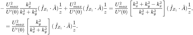 \begin{align} &
-\frac{U_{max}^{2}}{U^{\prime}(0)}\frac{k_{x}^{2}}{k_{x}^{2}+k_{y}^{2}}
(\,\hat{f}_{Z_{1}}\cdot\hat{A})\frac{1}{z}+\frac{U_{max}^{2}}{U^{\prime}(0)}
(\,\hat{f}_{Z_{1}}\cdot\hat{A})\frac{1}{z}=\frac{U_{max}^{2}}{U^{\prime}(0)}
\left[\frac{k_{x}^{2}+k_{y}^{2}-k_{x}^{2}}{k_{x}^{2}+k_{y}^{2}}\right]
(\,\hat{f}_{Z_{1}}\cdot\hat{A})\frac{1}{z}, \nonumber\\
&\quad
=\frac{U_{max}^{2}}{U^{\prime}(0)}\left[\frac{k_{y}^{2}}{k_{x}^{2}+k_{y}^{2}}\right]
(\,\hat{f}_{Z_{1}}\cdot\hat{A})\frac{1}{z}. \end{align}
\begin{align} &
-\frac{U_{max}^{2}}{U^{\prime}(0)}\frac{k_{x}^{2}}{k_{x}^{2}+k_{y}^{2}}
(\,\hat{f}_{Z_{1}}\cdot\hat{A})\frac{1}{z}+\frac{U_{max}^{2}}{U^{\prime}(0)}
(\,\hat{f}_{Z_{1}}\cdot\hat{A})\frac{1}{z}=\frac{U_{max}^{2}}{U^{\prime}(0)}
\left[\frac{k_{x}^{2}+k_{y}^{2}-k_{x}^{2}}{k_{x}^{2}+k_{y}^{2}}\right]
(\,\hat{f}_{Z_{1}}\cdot\hat{A})\frac{1}{z}, \nonumber\\
&\quad
=\frac{U_{max}^{2}}{U^{\prime}(0)}\left[\frac{k_{y}^{2}}{k_{x}^{2}+k_{y}^{2}}\right]
(\,\hat{f}_{Z_{1}}\cdot\hat{A})\frac{1}{z}. \end{align}
Substituting this simplified form of the singular terms and taking into account their inverse Fourier transform, we obtain a more compact form of the expression for  $u_{2}$
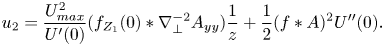 \begin{equation} u_{2}=\frac{U_{max}^{2}}{U^{\prime}(0)}(f_{Z_1}(0)\ast \nabla_{{\perp}}^{{-}2}A_{yy})\frac{1}{z}+ \frac{1}{2}(f\ast A)^{2}U^{\prime\prime}(0). \end{equation}
It is easy to see that uniformity of the main-deck asymptotic expansion breaks down as  $z\to 0$. Indeed, according to (3.43) and (3.41) unless the spanwise component dependence vanishes, velocity components $u_{2}$ and $v_{3}$ diverge
 \begin{equation} u_{2}\sim 1/z,\quad v_{3}\sim 1/z. \end{equation}
To get rid of the singularities, in Appendix A we re-scale the variables appropriately and solve the Navier–Stokes equations in the region immediately adjacent to the boundary (the lower deck) and then match these solutions with the solutions already obtained for the main deck. The main results of the detailed analysis carried out in Appendix A can be summarized as follows: (i) under the chosen scaling a uniformly valid explicit asymptotic solution has been found for the no-stress boundary layers, although in a quite complicated form; (ii) in the context of derivation of evolution equation the specific form of the solution in the viscous sub-layer is immaterial, since under adopted scaling the inner solution anyway does not affect the motion in the main deck and, hence, does not contribute to the evolution equation.
3.5. Conclusions
The main result of this section and of the paper is the novel nonlinear evolution equation (3.34) for long 3-D perturbations in semi-infinite boundary layers with explicit accounting of both weak stratification and viscous effects.
The evolution equation (3.38) provides the framework for studying dynamics of 3-D perturbations and, in particular, to clarify hitherto unexamined role of stratification ( $\tilde {\beta }_{2}\neq 0$) and Rayleigh friction, which is carried out in the follow-up companion paper.
4. Concluding remarks
Here, we briefly summarize the results of the work and discuss the new questions it generates. The work presents a new asymptotic model describing the nonlinear dynamics of linearly decaying 3-D long-wave perturbations in a generic semi-infinite weakly stratified free-surface boundary layer. The model, the first of its kind, is a generalization of the essentially 2-D Benjamin–Ono equation taking explicit account of new dispersion due to weak stratification in the boundary layer and dissipation. The account of dissipation in the boundary layer results in the Rayleigh friction-type term which is proportional to the ratio of the curvature of the basic flow vorticity at the boundary and the Reynolds number. The model is derived in the distinguished limit with nonlinearity, the two types of dispersion and dissipation all being in balance. This provides a possibility of reducing the evolution equation (3.38) to a family of simplified equations, each balanced in its own range of parameters. For example, for a wide range of the Reynolds numbers, the Rayleigh friction term could be dropped, which makes the dynamics described by the reduced equation Hamiltonian. For relatively short perturbations we recover 2-D-BO equation, while, for sufficiently long perturbations, we can neglect the Benjamin–Ono dispersion, which will result in a yet another novel equation with peculiar properties
 \begin{equation} A_{\tau}+AA_{x}-\tilde{\beta}_{2}\hat{G}_{2}[A_{x}]=0. \end{equation}
Here, the dispersion which is proportional to  $k_y^2/k_x^2$ does not depend on the wavenumber, it vanishes for the plane perturbations propagating strictly streamwise. Steady waves are impossible, since even for non-planar perturbations with non-vanishing dispersion, the dispersion cannot balance nonlinearity: counterintuitively, it decreases with nonlinear steepening of the perturbations. The non-trivial dynamics within the framework of the evolution equation (3.38) and its reductions is studied in the follow-up companion paper.
Here, we stress that the model (3.38) is self-contained: the evolution equation describes the dynamics of a single long-wave mode which is weakly decaying in the linear setting. Under the adopted scaling the weakly nonlinear dynamics in the critical layer is dominated by viscosity. This enables us to solve the nonlinear equations governing the critical layer. Crucially, in contrast to the no-slip setting, to leading order the lower deck does not affect the main deck, i.e. the critical layer dynamics does not affect the processes in the bulk of the boundary layer which we are primarily interested in.
The asymptotic derivation largely follows the earlier derivations (Shrira Reference Shrira1989; Voronovich et al. Reference Voronovich, Shrira and Stepanyants1998) of related evolution equations, with three important distinctions. First, the derivation has been extended to weakly stratified free-surface boundary layers with the no-stress boundary conditions at the surface, which resulted in an extra dispersion which, to the best of our knowledge, is novel. For sufficiently long perturbations the novel dispersion is dominant, which can change the dynamics qualitatively. Second, the range of the allowed Reynolds numbers was extended towards lower values, down to  ${Re}\sim \varepsilon ^{-2}$, which results in the Rayleigh friction-type term in the evolution equation. Third, the restriction which excluded the flow profiles with inflection points employed in the earlier derivations of related evolution equations was lifted. Viscous linear instabilities in no-stress boundary layers have been a priori excluded from consideration by our focus on linearly decaying perturbations, they might be relevant in certain contexts and will be considered elsewhere.
The work also raises many questions which currently remain open. The model itself is examined in the companion follow-up paper. Here, we just very briefly discuss the limitations of the model and how it can be extended. One of the obvious limitations is the total neglect of possible inhomogeneity of the basic flow and non-parallel effects. The assumption of spatial homogeneity with respect to horizontal coordinates allows both the direct and inverse Fourier transforms under easy to satisfy Dirichlet's conditions, which greatly facilitates the derivation. It is in principle possible to incorporate weakly inhomogeneous and non-parallel effects into the employed asymptotic scheme. This has been partly done in Shrira et al. (Reference Shrira, Caulliez and Ivonin2005) for a free-surface boundary layer in non-stratified fluid. However, a detailed investigation of these effects requires a dedicated study and goes beyond the scope of the present work. In contrast to the most of no-slip boundary layers in the laminar–turbulent transition, accounting for inhomogeneous and non-parallel effects is not the primary concern in the oceanic context, where most often there is a sufficient scale separation to make a homogeneous boundary layer a viable approximation.
To fix the idea the present work is confined to the simplest unidirectional generic boundary layer, but it also offers a possibility to extend the developed asymptotic approach to other types of no-stress boundary layers, such as 3-D boundary layers, confined boundary layers, situations with density stratification outside the boundary layer and with a compliant free-surface boundary. The extension of the derivation to these situations enables one to get a broad new class of novel nonlinear evolution equations which might prove of interest in other contexts as well. Although the general idea of how the extension of the derivation might work has been made clear, the derivation should be carried out from scratch in each case.
The prime motivation for undertaking this work was the desire to get a new insight into the physics of mixing in the oceanic upper layer. To this end we derived a model which in the context of this aim would be fair to refer to as a toy model. In its present form the model is applicable under benign conditions of gentle wind ( $U_{10}<4$ m s $^{-1}$) and moderate solar heating, when surface boundary layers are laminar and weakly stratified. Such situations are not uncommon, but from the viewpoint of ocean–atmosphere interaction are not the most interesting ones. Here, we will not speculate how the model might be extended for more challenging and more interesting, in this context, turbulent boundary layers. To what extent this work helps in closing the gap in our understanding of mixing mechanisms in the already turbulent oceanic boundary layer remains unclear. The key assumption that the dynamics of turbulent boundary layer can indeed be modelled by adopting the Boussinesq closure with constant scalar eddy viscosity remains to be verified. This requires a substantial dedicated effort and is beyond the scope of the present work. This model might be also relevant for describing a route to mixing in many other physical contexts with no-stress boundary layers, e.g. in engineering (e.g. Dasgupta, Nath & Bhanja Reference Dasgupta, Nath and Bhanja2019).
Throughout this work we assumed the surface tangential stress  $\boldsymbol {\tau }$ to be constant. In reality, wind always fluctuates, and the statistical properties of these fluctuations have been studied for many years (e.g. Jiménez Reference Jiménez2012; Yousefi, Veron & Buckley Reference Yousefi, Veron and Buckley2020). The airflow turbulence creates wind fluctuations with reasonably well-known statistical properties, which generates fluid motions beneath the water surface. To account for these motions it is straightforward to extend our evolution equation by adding a stochastic forcing due to fluctuations of $\boldsymbol {\tau }$. We expect that there is a range of temporal and spatial scales where the response in the water is dominated by the vorticity modes (1.5), even if the modes are weakly decaying, as is typical of other shear flows (e.g. Schmid & Henningson (Reference Schmid and Henningson2000), § 7.3). Our work highlights the existence of the modes with the dispersion relation (1.5). The dispersion relation, and hence the response, are sensitive to the properties of the boundary layer and, in particular, to the weak stratification. This makes these modes a serious contender for a role in remote sensing of the oceanic boundary layer. Although in this work we described the water surface as rigid, this is a simplification one can easily drop when necessary. Upon taking into account small but finite Froude numbers in the free-surface boundary condition it is straightforward to find the small free-surface displacements caused by the vorticity modes we study. The displacements, although tiny, might be probed remotely, since in the ocean there are no energetic motions with the same spatio-temporal characteristics. Another kind of surface signature of the studied vorticity waves is also possible. Inhomogeneities of surface velocity field due to the vorticity waves affect surface roughness and might create distinctive roughness signatures similar to those caused by internal gravity waves (e.g. Apel et al. Reference Apel, Byrne, Proni and Charnell1975). In the long term, tracing and deciphering the dynamics of such signatures might help in remote probing of the characteristics of the surface boundary layer inaccessible by other means. We hope that our work will stimulate new observations in subsurface boundary layers in laboratory facilities and natural water basins.
Acknowledgements
The authors are grateful to S.N. Timoshin and J.J. Healey for helpful discussions. The discussions with Y.S. Kachanov were instrumental in our decision to start this work.
Funding
The authors gratefully acknowledge the support of J. Oloo by the Commonwealth Scholarship Commission via grant KECA-2016-30, without which this work would not have happened. The work was also partly supported by UK NERC grants NE/R012202 and NE/S011420/1.
Declaration of interests
The authors report no conflict of interest.
Appendix A. Viscous sub-layer
Here, we solve the Navier–Stokes equations in the lower deck, i.e. in the viscous sub-layer, the region immediately adjacent to the boundary, and then match these inner solutions with the outer solutions already obtained for the main deck in § 3.4. Hence, the resulting matched asymptotic expansion will be uniformly valid by construction. We are using the terms ‘viscous sub-layer’ and ‘critical layer’ interchangeably, which is justified in our context.
Following Voronovich et al. (Reference Voronovich, Shrira and Stepanyants1998), we scale the critical layer thickness  $\delta$ as
 \begin{equation} \delta=(\varepsilon Re U_{0}^{\prime})^{{-}1/3}= (\varepsilon^{{-}1}Re_{{\ast}}U_{0}^{\prime})^{{-}1/3} \sim\varepsilon^{1/3} \quad (U_{0}^{\prime} =U^{\prime}|_{z=0},\quad Re_{{\ast}}=\varepsilon^{2}Re), \end{equation}
which ensures that  $\delta$ is small compared with the $O(1)$ overall thickness of the boundary layer $\delta _{BL}$. For further consideration it is crucial that
 \begin{equation} 1\gg \delta \gg \varepsilon, \end{equation}
which means that the thickness of viscous critical layer we are considering far exceeds the thickness of nonlinear critical layer, while it remains small compared with the boundary-layer thickness. The scaling specifies the regime where viscosity is dominant, while nonlinearity is small but finite and, hence, not negligible.
A.1. Re-scaling. Inner variable
To proceed, we re-scale our variables as follows:
 \begin{equation} \left.\begin{gathered} \xi=\frac{z}{\delta};\quad T=U_{0}^{\prime}\tau;\quad U-c=\delta U_{0}^{\prime}\xi+o(\delta);\quad N^{2}= (U_{0}^{\prime})^{2}\breve{N}^{2},\\ u=U_{0}^{\prime}\breve{u};\quad v=\frac{\varepsilon}{\delta}U_{0}^{\prime}\breve{v};\quad w=\delta U_{0}^{\prime}\breve{w};\quad p=\varepsilon(U_{0}^{\prime})^{2}\breve{p}. \end{gathered}\right\} \end{equation}
In terms of the new variables, after some algebra, the Navier–Stokes equations for  $w$ and other components of velocity take the form
 \begin{align} & \xi^{2}(U_{0}^{\prime})^{3}\partial_{xx}^{2}\partial_{\xi\xi}^{2}\breve{w}+2 \frac{\varepsilon}{\delta}\xi(U_{0}^{\prime})^{3} \partial_{xT}^{2}\partial_{\xi\xi}^{2}\breve{w}= \frac{\varepsilon}{\delta}\xi(U_{0}^{\prime})^{3}\partial_{\xi}\partial_{xx}^{2} \left[\breve{u}\partial_{x}\breve{u}+\breve{w}\partial_{\xi}\breve{u}\right] \nonumber\\ &\quad -\varepsilon(U_{0}^{\prime})^{3}Ri_{{\ast}}\nabla_{{\perp}}^{2} \breve{N}^{2}\breve{w}+\frac{(\varepsilon^{{-}1}Re_{{\ast}})^{{-}1}} {\delta^{3}}(U_{0}^{\prime})^{2}\partial_{x}\xi\partial_{\xi\xi\xi\xi}^{4}\breve{w}, \end{align}
 \begin{align} & (U_{0}^{\prime})^{2}\xi\partial_{x}\breve{u}+\frac{\varepsilon}{\delta} (U_{0}^{\prime})^{2}\partial_{T}\breve{u}+(U_{0}^{\prime})^{2}\breve{w}+ \frac{\varepsilon}{\delta}(U_{0}^{\prime})^{2}\breve{p}_{x} \nonumber\\ &\quad ={-}\frac{\varepsilon}{\delta}(U_{0}^{\prime})^{2}\left[\breve{u}\partial_{x}\breve{u}+ \frac{\varepsilon}{\delta}\breve{v}\partial_{y}\breve{u}+\breve{w}\partial_{\xi}\breve{u}\right]+ \frac{(\varepsilon^{{-}1}Re_{{\ast}})^{{-}1}}{\delta^{3}}U_{0}^{\prime}\partial_{\xi\xi}^{2}\breve{u}, \end{align}
 \begin{align} & \xi (U_{0}^{\prime})^{2}\partial_{x}\breve{v}+(U_{0}^{\prime})^{2} \frac{\varepsilon}{\delta}\partial_{T}\breve{v}+(U_{0}^{\prime})^{2}\breve{p}_{y} \nonumber\\ &\quad ={-}(U_{0}^{\prime})^{2}\left[\frac{\varepsilon}{\delta}\breve{u}\partial_{x}\breve{v}+ \left(\frac{\varepsilon}{\delta}\right)^{2}\breve{v}\partial_{y}\breve{v}+ \frac{\varepsilon}{\delta}\breve{w}\partial_{\xi}\breve{v}\right]+ \frac{(\varepsilon^{{-}1}Re_{{\ast}})^{{-}1}}{\delta^{3}}U_{0}^{\prime}\partial_{\xi\xi}^{2}\breve{v}, \end{align}
 \begin{align} &U_{0}^{\prime}\breve{u}_{x}+\frac{\varepsilon}{\delta}U_{0}^{\prime} \breve{v}_{y}+U_{0}^{\prime}\breve{w}_{\xi}=0. \end{align}
The only difference of the re-scaled equations above from those in Voronovich et al. (Reference Voronovich, Shrira and Stepanyants1998) is the  $O(\varepsilon )$ stratification term in (A4a). On eliminating $U_{0}^{\prime }$ and substituting $\delta =(\varepsilon ^{-1}U_{0}^{\prime }Re_{\ast })^{-1/3}$, where $Re_{\ast }=\varepsilon ^{2}Re$ is re-scaled Reynolds number, while retaining only the leading-order $O(1)$ terms and $\epsilon /\delta$ correction terms, equations (A4) can be written as
 $$\begin{gather} (\partial_{\xi\xi}^{2}-\xi\partial_{x})\breve{w}^{\prime\prime}= \frac{\varepsilon}{\delta}\left(2\partial_{T}\breve{w}^{\prime\prime}-\partial_{\xi} \partial_{x}(\breve{u}\breve{u}_{x}+\breve{w}\breve{u}_{\xi})\right), \end{gather}$$
 $$\begin{gather}(\partial_{\xi\xi}^{2}-\xi\partial_{x})\breve{u}=\breve{w}+ \frac{\varepsilon}{\delta}(\partial_{T}\breve{u}+\breve{p}_{x}+ \breve{u}\breve{u}_{x}+\breve{w}\breve{u}_{\xi}), \end{gather}$$
 $$\begin{gather}(\partial_{\xi\xi}^{2}-\xi\partial_{x})\breve{v}=\breve{p}_{y}+ \frac{\varepsilon}{\delta}(\partial_{T}\breve{v}+\breve{u}\breve{v}_{x}+\breve{w}\breve{v}_{\xi}), \end{gather}$$
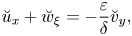 $$\begin{gather}\breve{u}_{x}+\breve{w}_{\xi}={-}\frac{\varepsilon}{\delta}\breve{v}_{y}, \end{gather}$$
where  $\breve {w}^{\prime \prime }=\partial _{\xi \xi }^{2}\breve {w}$, and $\breve {u},\breve {v},\breve {w},\breve {p}$ are the re-scaled dependent variables, while $T$ is re-scaled time. We re-iterate here that the quantities with breve symbol and the partial derivatives with respect to both $x$ and $y$ are treated as order-one quantities, since the explicit smallnesses due to $\varepsilon$ have all been pulled out. Therefore, in the above re-scaled Navier–Stokes equations we have only one small parameter, $\varepsilon /\delta \sim \varepsilon ^{2/3}$. We stress that, under the adopted scaling, the $O(\varepsilon )$ buoyancy term proportional to $\breve {N}^{2}$, proved to be negligible in the critical layer. Therefore, we are justified in retaining only the correction to leading order due to nonlinearity which is $\varepsilon /\delta \sim \varepsilon ^{2/3}$. However, the weak stratification does affect the dynamics of the viscous sub-layer through the matching conditions which we discuss later. With the buoyancy term dropped, these governing equations (A5) become identical to their counterparts in the Voronovich et al. (Reference Voronovich, Shrira and Stepanyants1998). The new small parameter $\varepsilon /\delta =\varepsilon ^{2/3}$, defined as the ratio of nonlinear critical layer width $\varepsilon$ to that of viscous critical layer width $\delta$, is the inverse of the Haberman number. Since (A5) have only the small parameter $\varepsilon /\delta$, we look for the solution of (A5) in the form of asymptotic power series in $\varepsilon /\delta$, rather than $\varepsilon$, subject to the no-stress boundary conditions at the boundary and matching conditions at infinity.
The formulation of the boundary value problem in the viscous sub-layer is completed by complementing (A5) with the no-flux condition at the boundary  $\xi =0$
 \begin{equation} \breve{w}=0, \end{equation}
and the no-stress condition at  $\xi =0$,
 \begin{equation} \breve{u}^{\prime}=\breve{v}^{\prime}=0. \end{equation}
 The inner solutions at  $\xi \to \infty$ should match the main-deck solutions taken at $z \to 0$, which, in terms of inner variable $\xi$, implies
 $$\begin{gather} \breve{u}\rightarrow-A + \frac{\varepsilon}{\delta} {\mathcal{P}}_{yy}{\frac{1}{\xi}}, \end{gather}$$
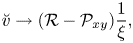 $$\begin{gather}\breve{v}\rightarrow {({\mathcal{R}}- {\mathcal{P}}_{xy}){\frac{1}{\xi}}}, \end{gather}$$
 $$\begin{gather}\breve{w} \rightarrow A_x \xi +\frac{\varepsilon}{\delta} \left(A_{T} - \nabla_{{\perp}}^{2}{\mathcal{P}}_{x} - AA_x+\frac{1}{Re_{{\ast}}} \left[\frac{U^{\prime\prime\prime}(0)}{(U^{\prime}(0))^{2}}\right]A+ \left[\frac{N_{0}^{2}}{2(U^{\prime}(0))^{2}}\right]\hat{G}_{2}[A_{x}]\right), \end{gather}$$
 $$\begin{gather}\breve{p} \rightarrow {\mathcal{P}}_{xx}-{\mathcal{R}}, \end{gather}$$
 $$\begin{gather}{\mathcal{P}}=\left(\frac{U_{max}}{U^{\prime}(0)}\right)^2\left(f_{Z_{1}}* \nabla_{{\perp}}^{{-}2}A\right),\quad {\mathcal{R}}=\frac{N_{0}^{2}}{2(U^{\prime}(0))^{2}}\hat{G}_{3}[A], \end{gather}$$
where  $\hat {G}_{2}$ and $\hat {G}_{3}$ are integral operators introduced in (§ 3). In the Fourier space, the integral operators $\hat {G}_{2}$ and $\hat {G}_{3}$ are, respectively, just multiplication operators ${k_{y}^{2}}/{k_{x}^{2}}$, while $\hat {G}_{3}={k_{y}^{3}}/{k_{x}^{3}}$.
A similar, but slightly less general, boundary value problem has been considered in Voronovich et al. (Reference Voronovich, Shrira and Stepanyants1998). Here, we provide the solution in a somewhat different form in terms of the classical Airy functions and their integrals for a broader range of the Reynolds numbers. In contrast to Voronovich et al. (Reference Voronovich, Shrira and Stepanyants1998), here we also allow the weak stratification to alter the dynamics in the critical layer through the matching with the stratification-dependent main-deck solution.
A.2. The inner solution in the critical layer and its matching with the outer solution of the main deck
A.2.1. Asymptotic expansion
We seek solution to the above boundary value problem in terms of an asymptotic series in  $\varepsilon /\delta$
 $$\begin{gather} \breve{u}= \breve{u}_{0} + \frac{\varepsilon}{\delta}\breve{u}_{1}+ \cdots, \end{gather}$$
 $$\begin{gather}\breve{v}=\breve{v}_{0} + \frac{\varepsilon}{\delta}\breve{v}_{1}+ \cdots, \end{gather}$$
 $$\begin{gather}\breve{w}=\breve{w}_{0} + \frac{\varepsilon}{\delta}\breve{w}_{1}+ \cdots, \end{gather}$$
 $$\begin{gather}\breve{p}=\breve{p}_{0} + \frac{\varepsilon}{\delta}\breve{p}_{1}+ \cdots . \end{gather}$$
A.2.2. Leading-order solutions $\breve {w}_{0}$ and $\breve {u}_{0}$


In this section we solve the Navier–Stokes equations (A5) using the asymptotic series (A9). To leading order in  ${\varepsilon }/{\delta }$ we obtain a linear boundary value problem because the scaling we adopted ensures that viscosity dominates nonlinearity in the viscous sub-layer. It is easy to see that, to leading order in $\varepsilon /\delta$, (A5a) is a fourth-order homogeneous linear ordinary differential equation of the form
 \begin{equation} (\partial_{\xi\xi}^{2}-\xi\partial_{x})\breve{w}_{0}^{\prime\prime}=0. \end{equation}
It is also fairly straightforward to see that
 \begin{equation} \breve{w}_{0}=C\xi, \end{equation}
is a particular solution to (A10) satisfying the no-flux condition  $\breve {w}_{0}=0$ at $\xi =0$, with $C$ being an arbitrary integration constant. Hereinafter in this section, unless explicitly specified otherwise, the ‘constants’ are understood as quantities not depending on $\xi$, while retaining unspecified dependence on $x, y, T$. This constant is specified as $A_x$ by matching the found particular solution (A11) with the leading order of the expression for $\breve {w}$ in (A8c) as $\xi \to \infty$. The general solution to (A10) contains three other arbitrary constants which for the chosen particular solution are all set to be zero. On substituting ansatz (A11) into (A5b) and retaining just the leading-order terms we immediately obtain an inhomogeneous Airy equation for $\breve {u}_{0}$ with the right-hand side term dependent on $\xi$
$\xi$
 \begin{equation} (\partial_{\xi\xi}^{2}-\xi\partial_{x})\breve{u}_{0}=A_{x}\xi. \end{equation}
It is easy to see that  $\breve {u}_{0}=-A$ is a particular solution of (A12) satisfying to leading order the matching condition (A8a) as $\xi \to \infty$. Therefore, we conclude our brief analysis in this section by outlining the found simple solutions for the no-stress boundary satisfying both the governing equations and matching condition, i.e.
 \begin{equation} \breve{u}_{0}={-}A,\quad \breve{w}_{0}=A_{x}\xi. \end{equation}
The zero-order solution for  ${\breve {v}}_{0}(\xi )$ will be derived later, once pressure $\breve {p}_{0}$ is found. These solutions were first found in Voronovich et al. (Reference Voronovich, Shrira and Stepanyants1998) for the same boundary conditions. Here, we provide the derivation, since we will need it for the next steps.
A.3. First-order solutions
The found particular leading-order solutions  $\breve {u}_{0}=-A$ and $\breve {w}_{0}=A_{x}\xi$ have a remarkable property: as we show below, on substituting these solutions into (A5a), it immediately follows that the $O(\varepsilon /\delta )$ right-hand side vanishes and we get for $\partial _{\xi \xi }^{2}\breve {w}_{1}$ the homogeneous Airy equation identical to the equation for $\breve {w}_{0}$.
A.3.1. Equation for $\breve {w}_{1}$

Consider more closely the right-hand side  ${\mathcal {R}}_1$ of the equation for $\breve {w}^{\prime \prime }_1$
 \begin{equation} (\partial_{\xi\xi}^{2}-\xi\partial_{x})\breve{w}_{1}^{\prime\prime} ={\mathcal{R}}_1,\quad {\mathcal{R}}_1=\frac{\varepsilon}{\delta} \left(2\partial_{T}\breve{w}_{0}^{\prime\prime}-\partial_{\xi}\partial_{x} (\breve{u}_{0}\breve{u}_{0x}+\breve{w}_{0}\breve{u}_{0\xi})\right). \end{equation}
Let us first simplify  ${\mathcal {R}}_1$ using the already found leading-order solutions $\breve {u}_{0}(\xi )$ and $\breve {w}_{0}(\xi )$. It is easy to see that the first term, $\partial _{T}\breve {w}_{0}^{\prime \prime }$, vanishes because $\breve {w}_{0}$ is linear in $\xi$. Next, we simplify the second term in ${\mathcal {R}}_1$ inside the brackets. We stress that at this step there is no loss of generality and no specific form of $\breve {u}_{0}(\xi )$ is used. To leading order the continuity equation (A5d) is one-dimensional
 \begin{equation} \breve{u}_{0x}={-}\breve{w}_{0\xi},\quad \breve{w}_{0}=A_{x}\xi. \end{equation}
Therefore
 \begin{align} \partial_{x}\partial_{\xi}(\breve{u}_{0}\breve{u}_{0x}+ \breve{w}_{0}\breve{u}_{0\xi})=\partial_{x}\partial_{\xi} (-\breve{u}_{0}A_{x}+A_{x}\xi\breve{u}_{0\xi})=A_{xx}(-\breve{u}_{0\xi}+ \breve{u}_{0\xi}+\xi\breve{u}_{0\xi\xi})=A_{xx}\xi\breve{u}_{0\xi\xi}. \end{align}
On substituting this simplifications of  ${\mathcal {R}}_1$ into (A13a,b), we re-write it in a much simpler form:
 \begin{equation} (\partial_{\xi\xi}^{2}-\xi\partial_{x})\breve{w}_{1}^{\prime\prime} ={-}A_{xx}\xi\breve{u}_{0\xi\xi}. \end{equation}
 By virtue of (A13a,b)  $\breve {u}_{0}$ does not depend on $\xi$, $\breve {u}_{0\xi \xi } =0.$ This reduces (A13a,b) to the homogeneous equation for $\breve {w}_{1}$
 \begin{equation} (\partial_{\xi\xi}^{2}-\xi\partial_{x})\breve{w}_{1}^{\prime\prime}=0. \end{equation}
Hence, we have to solve the same fourth-order homogeneous linear differential equation (A10) as for the leading-order  $\breve {w}_{0}$. However, we cannot set $\breve {w}_{1}$ to be zero or incorporate it into $\breve {w}_{0}$, since, by virtue of (A8c), it has a different asymptotics as $\xi \to \infty$, in contrast to linearly growing $\breve {w}_{0}$, $\breve {w}_{1}$ tends to a constant.
A.3.2. Solution for $\breve {w}_{1}$

On performing the Fourier transform of (A18) and recalling that in the Fourier space  $\partial _{x}$ yields $\textrm {i}k_{x}$, we obtain
 \begin{equation} (\partial_{\xi\xi}^{2}-\xi {\rm i}k_{x})\hat{\breve{w}}_{1}^{\prime\prime}=0. \end{equation}
To proceed, we first introduce an auxiliary function  $S=\hat {\breve {w}}_{1}^{\prime \prime }$ and re-write (A19) as
 \begin{equation} (\partial_{\xi\xi}^{2}-\xi {\rm i}k_{x})S=0. \end{equation}
The general solution to (A20) is a superposition of the Airy functions with two arbitrary constants  $C_{1}$ and $C_{2}$
 \begin{equation} S(\xi)=C_{1}{\rm Ai}\left[({\rm i}k_{x})^{1/3}\xi\right]+C_{2}{\rm Bi}\left[({\rm i}k_{x})^{1/3}\xi\right]. \end{equation}
To find  $\hat {\breve {w}}_{1}$ we integrate solution (A21) twice. The solution we obtain contains four arbitrary constants $C_{1},C_{2},C_{3}$ and $C_{4}$
 \begin{align} \hat{\breve{w}}_{1} &= C_{1}\int_{0}^{\xi}\left[\int_{0}^{s_{2}}{\rm Ai} \left[({\rm i}k_{x})^{1/3}s_{1}\right]\mathrm{d}s_{1}\right]\mathrm{d}s_{2}+ C_{2}\int_{0}^{\xi}\left[\int_{0}^{s_{4}}{\rm Bi}\left[({\rm i}k_{x})^{1/3}s_{3}\right] \mathrm{d}s_{3}\right]\mathrm{d}s_{4} \nonumber\\ &\quad +C_{3}\xi+C_{4}, \end{align}
where  $s_{1},s_{2},s_{3}$ and $s_{4}$ are dummy variables. We set $C_{2}=0$, since the term containing the integral of $Bi$ diverges exponentially as $\xi \to \infty$. Hence, the solution for $\hat {\breve {w}}_{1}$ becomes
 \begin{equation} \hat{\breve{w}}_{1}=C_{1}\int_{0}^{\xi} \left[\int_{0}^{s_{2}}{\rm Ai}\left[({\rm i}k_{x})^{1/3}s_{1}\right] \mathrm{d}s_{1}\right]\mathrm{d}s_{2}+C_{3}\xi+C_{4}. \end{equation}
Applying the formula for the double integral of the Airy function (e.g. Olver et al. (Reference Olver, Lozier, Boisvert and Clark2010), (9.10.20)) we re-write the solution (A23) as follows:
 \begin{align} \hat{\breve{w}}_{1} &= C_{1}\left[\xi\int_{0}^{\xi}{\rm Ai} \left[({\rm i}k_{x})^{1/3}s_{2}\right]\mathrm{d}s_{2}-({\rm i}k_{x})^{1/3}{\rm Ai}^{\prime} \left[({\rm i}k_{x})^{1/3}\xi\right]+({\rm i}k_{x})^{1/3}{\rm Ai}^{\prime}(0)\right] \nonumber\\ &\quad +C_{3}\xi+C_{4}. \end{align}
Requiring  $\hat {\breve {w}}_{1}$ to satisfy the no-flux condition at $\xi =0$ dictates $C_{4}=0$.
Let us take a closer look at the terms in the square brackets of (A24). Noting that for  $\xi \to \infty$ the integral equals $1/(3(\textrm {i}k_{x})^{1/3})$ (Olver et al. (Reference Olver, Lozier, Boisvert and Clark2010), (9.10.11) and (9.10.1)), then the large $\xi$ asymptotics of solution (A24) can be presented as
 \begin{equation} \hat{\breve{w}}_{1}=\frac{1}{3({\rm i}k_{x})^{1/3}}C_{1} \xi-C_{1}({\rm i}k_{x})^{1/3}{\rm Ai}^{\prime}\left[({\rm i}k_{x})^{1/3}\xi\right] +C_{1}({\rm i}k_{x})^{1/3}{\rm Ai}^{\prime}(0)+C_{3}\xi. \end{equation}
The matching condition (A5c) requires  $\hat {\breve {w}}_{1}\to constant$ as $\xi \to \infty$. Since the large $\xi$ asymptotics (A25) of $\hat {\breve {w}}_{1}$ diverges linearly as $\xi \to \infty$, we set $C_{1}=-3(\textrm {i}k_{x})^{1/3}C_{3}$, which eliminates this divergence. Substituting $C_{1}=-3(\textrm {i}k_{x})^{1/3}C_{3}$ into (A25) and taking into account the vanishing derivative of the Airy function $Ai^{\prime }$ at $\xi \to \infty$, we obtain a solution for $\hat {\breve {w}}_{1}$, that tends to a constant as $\xi \to \infty$
 \begin{equation} \left.\begin{gathered} \hat{\breve{w}}_{1}|_{\xi \to \infty}={-}3({\rm i}k_{x})^{1/3}C_{3}{\rm Ai}^{\prime}(0)=\hat{C}=constant,\\ {\rm Ai}^{\prime}(0)={-}\frac{3^{1/6}\varGamma{\left(\dfrac{2}{3}\right)}}{2{\rm \pi}}={-}\frac{1}{3^{1/3}\varGamma{\left(\dfrac{1}{3}\right)}}. \end{gathered}\right\} \end{equation}
Matching the derived inner solution of the viscous sub-layer to the outer solution requires  $\hat {\breve {w}}_{1}=\hat {C}(\boldsymbol k, T)$. This specifies the value of this constant in the $\boldsymbol x$-space by virtue of (A8c),
 \begin{equation} \left.\begin{gathered} C= \left(A_{T} -\nabla_{{\perp}}^2{\mathcal{P}}_{x} - AA_x+\frac{1}{Re_{{\ast}}}\left[\frac{U_{0}^{\prime\prime\prime}} {(U_{0}^{\prime})^{2}}\right]A-\left[\frac{N_{0}^{2}}{2(U^{\prime}(0))^{2}}\right] \hat{G}_{2}[A_{x}]\right),\\ {\mathcal{P}} =\left(\frac{U_{max}}{U^{\prime}(0)}\right)^2 \left(f_{Z_{1}}\ast\nabla_{{\perp}}^{{-}2}A\right), \end{gathered}\right\} \end{equation}
where the specific value of the constant  $\hat {C}(\boldsymbol k, T)$ of (A26) is obtained by taking the Fourier transform of (A27)
 \begin{equation} \hat{C}=\mathcal{F}\{C\}. \end{equation}
 Thus, we have specified all the arbitrary constants in the derived solution (A24) for  $\hat {\breve {w}}_{1}$ that satisfies boundary and matching conditions. Finally, the solution for $\hat {\breve {w}}_{1}$ is
 \begin{equation} \hat{\breve{w}}_{1}=\frac{\hat{C}}{{\rm Ai}^{\prime}(0)} \left[\xi{\mathcal{I}}-({\rm i}k_{x})^{1/3}\mathrm{Ai}^{\prime}(Z)+ ({\rm i}k_{x})^{1/3}{\rm Ai}^{\prime}(0)-\frac{1}{3({\rm i}k_{x})^{1/3}}\xi\right], \end{equation}
where
 \begin{equation} {\mathcal{I}}=\int_{0}^{\xi}{\rm Ai}\left[({\rm i}k_{x})^{1/3}s_{2}\right] \mathrm{d}s_{2},\quad Z=({\rm i}k_{x})^{1/3}\xi, \end{equation}
A.3.3. Equation for $\breve {u}_{1}$

Here, we proceed to finding the streamwise component of the perturbation velocity  $\breve {u}_{1}$ from the Navier–Stokes equations (A5b). Recall, that $\breve {u}_{1}$ is diverging in the outer solution. On applying regular perturbations and retaining $O(\varepsilon /\delta )$ terms we obtain the governing equation for $\breve {u}_{1}$
 \begin{equation} (\partial_{\xi\xi}^{2}-\xi\partial_{x})\breve{u}_{1}= \breve{w}_{1}+\partial_{T}\breve{u}_{0}+\breve{p}_{0x}+ \breve{u}_{0}\breve{u}_{0x}+\breve{w}_{0}\breve{u}_{0\xi}. \end{equation}
The last term of the above equation vanishes by virtue of (A13a,b).
Recall the expressions for  $\breve {w}_{0},\breve {u}_{0}$ and $\breve {w}_{1}$
 \begin{equation} \left.\begin{gathered} \breve{u}_{0}={-}A,\quad \breve{w}_{0}=A_x\xi.\\ \breve{w}_{1}=A_{T}-\nabla_{{\perp}}^{2}{\mathcal{P}}_{x}-AA_{x}+ \frac{1}{Re_{{\ast}}}\left[\frac{U^{\prime\prime\prime}(0)}{(U^{\prime}(0))^{2}} \right]A+\left[\frac{N_{0}^{2}}{2(U^{\prime}(0))^{2}}\right] \hat{G}_{2}[A_{x}], \end{gathered}\right\} \end{equation}
where
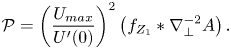 \begin{equation} {\mathcal{P}} =\left(\frac{U_{max}}{U^{\prime}(0)}\right)^2 \left(f_{Z_{1}}\ast\nabla_{{\perp}}^{{-}2}A\right). \end{equation}
On substituting these expressions for  $\breve {u}_{0}$, $\breve {w}_{0}$ and $\breve {w}_{1}$ into (A31) and carrying out further simplification, we get a much simplified equation for $\breve {u}_{1}$
 \begin{equation} (\partial_{\xi\xi}^{2}-\xi\partial_{x})\breve{u}_{1}={-}\nabla_{{\perp}}^{2}{\mathcal{P}}_{x}+ \frac{1}{Re_{{\ast}}}\left[\frac{U^{\prime\prime\prime}(0)}{(U^{\prime}(0))^{2}}\right]A+ \left[\frac{N_{0}^{2}}{2(U^{\prime}(0))^{2}}\right]\hat{G}_{2}[A_{x}]+\breve{p}_{0x}. \end{equation}
The above equation (A34) for  $\breve {u}_{1}$ includes $\breve {p}_{0}$, which has to be found prior to solving (A34). Pressure does not vary across the the critical layer and therefore can be determined by matching with the pressure term of the outer solution. That is, to find $\breve {p}_{0}$ inside the critical layer we match the boundary layer pressure solution $p_{3}$ (see (3.26))
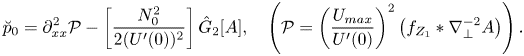 \begin{equation} \breve{p}_{0}=\partial_{xx}^{2}{\mathcal{P}}- \left[\frac{N_{0}^{2}}{2(U^{\prime}(0))^{2}}\right]\hat{G}_{2}[A],\quad \left({\mathcal{P}} =\left(\frac{U_{max}}{U^{\prime}(0)}\right)^2 \left(f_{Z_{1}}\ast\nabla_{{\perp}}^{{-}2}A\right)\right). \end{equation}
On substituting (A35a,b) into (A34), the buoyancy terms cancel out, hence, we find the streamwise velocity perturbations  $\breve {u}_{1}$ from the following inhomogeneous Airy equation with the right-hand side independent of $\xi$:
 \begin{equation} (\partial_{\xi\xi}^{2}-\xi\partial_{x})\breve{u}_{1}={-}{\mathcal{P}}_{xyy}+\frac{1}{Re_{{\ast}}} \left[\frac{U^{\prime\prime\prime}(0)}{(U^{\prime}(0))^{2}}\right]A, \end{equation}
where
 \begin{equation} {\mathcal{P}}=\left(\frac{c}{U^{\prime}(0)}\right)^{2} (f_{Z_{1}}(0)\ast\nabla_{{\perp}}^{{-}2}A),\quad c=U_{max}. \end{equation}
The expressions above differ from those obtained in Voronovich et al. (Reference Voronovich, Shrira and Stepanyants1998) by the account of the viscous effect inside the main deck, which yields the term with  $Re_{\ast }$ on the right-hand side of (A36). Note that, under the adopted scaling, viscous effects contribute into the equation for the perturbation velocity streamwise component $\breve {u}_{1}$, but, as we show below, do not affect the spanwise component $\breve {v}_{0}$. In contrast, we will show in the next section that, counterintuitively, stratification affects the spanwise component of the velocity $\breve {v}_{0}$, but not its streamwise counterpart $\breve {u}_{1}$.
A.3.4. Solution for $\breve {u}_{1}$

Here, we solve the inhomogeneous Airy equation with the right-hand side independent of  $\xi$. To find solution to (A36) we perform the Fourier transform with respect to independent variables $x$ and $y$. Recall that the operations of differentiation and integration we encounter in the $\boldsymbol x$-space and in the Fourier space are related as follows:
 \begin{equation} \partial_{x} \Leftrightarrow {\rm i}k_{x},\quad \partial_{y} \Leftrightarrow {\rm i}k_{y},\quad \nabla_{{\perp}}^{2}\Leftrightarrow -(k_{x}^{2}+k_{y}^{2})={-}k^{2},\quad \nabla_{{\perp}}^{{-}2}\Leftrightarrow -\frac{1}{k^{2}}. \end{equation}
Recall also that,  $\partial _{Z_{1}}{f}_{k}(0) \Leftrightarrow k=|\boldsymbol {k}|$ and $f(0) =1$, and
 \begin{equation} {\mathcal{P}}=\left(\frac{U_{max}}{U^{\prime}(0)}\right)^{2}(f_{Z_{1}}(0)\ast\nabla_{{\perp}}^{{-}2}A),\quad \implies\hat{{\mathcal{P}}}(\boldsymbol{k})={-}\frac{1}{k} \left(\frac{U_{max}}{U^{\prime}(0)}\right)^{2}\hat{A}(\boldsymbol{k}). \end{equation}
Substituting (A38a–d) and (A38a–d) in (A36) yields the following inhomogeneous Airy equations for the Fourier components  $\hat {\breve {u}}_{1}$ with the right-hand side independent of $\xi$:
 \begin{equation} (\partial_{\xi\xi}^{2}-{\rm i}k_{x}\xi)\hat{\breve{u}}_{1}={-}{\rm i}\frac{k_{x}k_{y}^{2}}{k} \left(\frac{c}{U^{\prime}(0)}\right)^{2}\hat{A}(\boldsymbol{k})+ \frac{1}{Re_{{\ast}}}\left[\frac{U^{\prime\prime\prime}(0)}{(U^{\prime}(0))^{2}}\right] \hat{A}(\boldsymbol{k}). \end{equation}
Its general solution expressed in terms of the Airy and Scorer functions can be found by the method of variation of parameters
 \begin{equation} \hat{\breve{u}}_{1}(\xi)=d_{1}\mathrm{Ai}(Z)+d_{2}\mathrm{Bi}(Z) + {\rm \pi}\hat{B}\hat{A}(\boldsymbol{k})g(Z), \end{equation}
where
 \begin{equation} \hat{B}={\rm \pi}\left[\frac{({\rm i}k_{x})^{1/3}k_{y}^{2}}{k} \left(\frac{c}{U^{\prime}(0)}\right)^{2}+\frac{({\rm i}k_{x})^{{-}2/3}}{Re_{{\ast}}} \left[\frac{U^{\prime\prime\prime}(0)}{(U^{\prime}(0))^{2}}\right]\right],\quad Z=({\rm i}k_{x})^{1/3}\xi, \end{equation}
while  $d_{1}, d_{2}$ are arbitrary constants. The Airy functions $\mathrm {Ai}(Z)$ and $\mathrm {Bi}(Z)$ are two fundamental solutions of the homogeneous Airy equation and $g(Z)$ is a particular solution of (A40). The particular solutions can be expressed in terms of the Scorer functions $\mathrm {Gi}(Z)$ and $\mathrm {Hi}(Z)$ (Olver et al. (Reference Olver, Lozier, Boisvert and Clark2010), (9.12.4), (9.12.5))
 \begin{equation} \left.\begin{gathered} \mathrm{Gi}(Z)=\mathrm{Bi}(Z)\int_{Z}^{\infty} \mathrm{Ai}(t)\,\mathrm{d}t+\mathrm{Ai}(Z) \int_{0}^{Z}\mathrm{Bi}(t)\,\mathrm{d}t,\\ \mathrm{Hi}(Z)=\mathrm{Bi}(Z)\int_{-\infty}^{Z} \text{Ai}(t)\,\mathrm{d}t-\mathrm{Ai}(Z)\int_{-\infty}^{Z}\mathrm{Bi}(t)\,\mathrm{d}t. \end{gathered}\right\} \end{equation}
We look for solutions satisfying the no-stress boundary conditions at  $\xi =0$ and matching with the outer solution at $\xi \to \infty$. By setting $d_{2}=0$ we eliminate the divergence in (A41) as $\xi \to \infty$ due to the term $\mathrm {Bi}(Z)$. Thus, we are left with the sum of the $\mathrm {Ai}$ component of the homogeneous solution and a particular solution expressed in terms of the Scorer functions. The asymptotic behaviour of the Scorer functions for large $\xi$ is (e.g. Olver et al. (Reference Olver, Lozier, Boisvert and Clark2010), (9.12.25), (9.12.27))
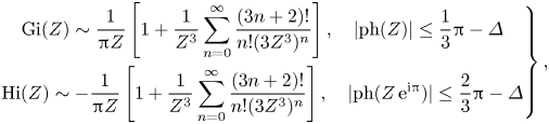 \begin{equation} \left.\begin{gathered} \mathrm{Gi}(Z)\sim\frac{1}{{\rm \pi} Z}\left[1+\frac{1}{Z^{3}} \sum_{n=0}^{\infty}\frac{(3n+2)!}{n!(3Z^{3})^{n}}\right],\quad |\mathrm{ph}(Z)|\le \frac{1}{3}{\rm \pi}-\varDelta\\ \mathrm{Hi}(Z)\sim{-}\frac{1}{{\rm \pi} Z}\left[1+\frac{1}{Z^{3}}\sum_{n=0}^{\infty} \frac{(3n+2)!}{n!(3Z^{3})^{n}}\right],\quad |\mathrm{ph} (Z\,{\rm e}^{{\rm i}{\rm \pi}})|\le \frac{2}{3}{\rm \pi}-\varDelta \end{gathered}\right\}, \end{equation}
where  $\varDelta$ is an arbitrary small positive constant.
Thus, both  $\mathrm {Gi}(Z)$ and $\mathrm {Hi}(Z)$ decay as $Z^{-1}$ as $\xi \to \infty$, but in different sectors of the complex plane. On the $Z$-plane the sector of validity for the Scorer function $\mathrm {Gi}$ includes positive wavenumbers $k_{x}>0$, but not $k_{x}<0$. Therefore, we discard it and retain only the $\mathrm {Hi}$ solution which has a much wider sector of validity, the explicit large $\xi$ expansion given above is valid for both $k_{x}<0$ and $k_{x}>0$. Thus, on discarding the contribution of $\mathrm {Gi}(Z)$ we obtain
 \begin{equation} \hat{\breve{u}}_{1}=\hat{B}\hat{A}(\boldsymbol{k})[\alpha_{k}\mathrm{Ai}(Z)+\mathrm{Hi}(Z)], \end{equation}
where
 \begin{equation} \hat{B}={\rm \pi}\left[\frac{({\rm i}k_{x})^{1/3}k_{y}^{2}}{k} \left(\frac{c}{U^{\prime}(0)}\right)^{2}+\frac{({\rm i}k_{x})^{{-}2/3}}{Re_{{\ast}}} \left[\frac{U^{\prime\prime\prime}(0)}{(U^{\prime}(0))^{2}}\right]\right]. \end{equation}
Thus,  $\hat {B}$ is determined by the matching condition (A8a), while the unspecified yet arbitrary constant $\alpha _{k}$ will be determined below by applying the no-stress condition at $\xi =0$. To this end consider the Maclaurin series of $\mathrm {Hi}(Z)$ at $\xi \to 0$ (Olver et al. (Reference Olver, Lozier, Boisvert and Clark2010), (9.12.17))
 \begin{equation} \mathrm{Hi}(Z)=\frac{3^{{-}2/3}}{\rm \pi}\sum_{n=0}^{\infty} \varGamma\left(\frac{n+1}{3}\right)\frac{(3^{1/3}Z)^{n}}{n!}, \end{equation}
where  $\varGamma (s)$ is the gamma function. As $\xi \to 0$ $\mathrm {Hi}(Z)$ tends to a constant
 \begin{equation} \mathrm{Hi}(\xi=0)=\frac{3^{{-}2/3}}{\rm \pi}\varGamma{\left(\frac{1}{3}\right)}= \frac{3^{{-}2/3}}{2{\rm \pi}}\varGamma{(1/3)}=\frac{2}{3^{7/6}\varGamma{\left(\dfrac{2}{3}\right)}}. \end{equation}
Since in the no-stress case  $u^{\prime }=v^{\prime }=0$ at $\xi =0$
 \begin{equation} \hat{B}\hat{A}\left(({\rm i}k_{x})^{1/3}\mathrm{Hi}^{\prime}(Z)+({\rm i}k_{x})^{1/3} \alpha_{k}\mathrm{Ai}^{\prime}(Z)\right)=0. \end{equation}
Hence, we specify coefficient  $\alpha _{k}$ by standard renormalization of Airy and Scorer functions as
 \begin{equation} \left.\begin{gathered} \alpha_{k}={-}\left.\frac{\mathrm{Hi}^{\prime}(Z)}{\mathrm{Ai}^{\prime}(Z)}\right|_{\xi=0}= \frac{2}{\sqrt{3}},\quad \mathrm{Hi}^{\prime}(\xi=0)=\frac{2}{3^{5/6} \varGamma{\left(\dfrac{1}{3}\right)}},\\ \mathrm{Ai}^{\prime}(\xi=0)={-}\frac{1}{3^{1/3}\varGamma{\left(\dfrac{1}{3}\right)}}. \end{gathered}\right\} \end{equation}
Thus, the solution for  $\hat {\breve {u}}_{1}$ is given in closed form by (A45). It is regular everywhere. The solution is a sum of the Airy function $\mathrm {Ai}(Z)$ contributed by the homogeneous Airy equation and the ‘inhomogeneous’ contribution described by the Scorer function $\mathrm {Hi}(Z)$. The Airy function contribution vanishes as $\xi \to \infty$ and does not contribute to matching with the outer solution. The Scorer function $\mathrm {Hi}(Z)$ for large values of its argument behaves as $Z^{-1}$ and is matched with the outer solution at $\xi \to \infty$, which specifies constant $\hat {B}$ in (A45). The only role of the Airy function contribution is to satisfy the no-stress conditions at $\xi =0$, which is ensured by our choice of $\alpha _{k}$.
To summarize our findings in this section, the Airy function  $\mathrm {Ai}(Z)$ decays exponentially as $\xi \to \infty$ and does not contribute to matching, while the Scorer function $\mathrm {Hi}$ in this limit tends to $Z^{-1}$. Consequently, the solution (A45) is matched to the outer solutions. Thus, the apparent singularities in the main-deck solutions are eliminated, while the critical layer contribution to nonlinear evolution in the main deck remains negligible.
A.3.5. Solution for $\breve {v}_{0}$

In this section we solve the Navier–Stokes equation (A5c) to find the leading-order solution for the spanwise perturbation velocity  $\breve {v}_{0}$. In contrast to the streamwise velocity component ${\breve {u}}_{1}$, the spanwise component of velocity $\breve {v}_{0}$ is unaffected by viscosity, but is modified by stratification $N_{0}^{2}$ via matching with the main deck constant pressure term of ((3.26)). Therefore, the resulting equation differs from its counterpart in Voronovich et al. (Reference Voronovich, Shrira and Stepanyants1998) (see (47))
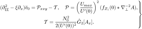 \begin{equation} \left.\begin{gathered} (\partial_{\xi\xi}^{2}-\xi\partial_{x})\breve{v}_{0}={\mathcal{P}}_{xxy}-{\mathcal{T}},\quad {\mathcal{P}}=\left(\frac{U_{max}}{U^{\prime}(0)}\right)^{2}(f_{Z_{1}}(0)\ast\nabla_{{\perp}}^{{-}2}A),\\ {\mathcal{T}}=\frac{N_{0}^{2}}{2(U^{\prime}(0))^{2}}\hat{G}_{2}[A_{x}]. \end{gathered}\right\} \end{equation}
In the Fourier space the resulting equation (A50a–c) for  $\hat {\breve {v}}_{0}$ is the inhomogeneous Airy equation with the right-hand side independent of $\xi$
$\xi$
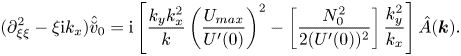 \begin{equation} (\partial_{\xi\xi}^{2}-\xi {\rm i}k_{x})\hat{\breve{v}}_{0}= {\rm i}\left[\frac{k_{y}k_{x}^{2}}{k} \left(\frac{U_{max}}{U^{\prime}(0)}\right)^{2}-\left[\frac{N_{0}^{2}}{2(U^{\prime}(0))^{2}}\right] \frac{k_{y}^{2}}{k_{x}}\right]\hat{A}(\boldsymbol{k}). \end{equation}
This equation can be solved using the method of variation of parameters similarly to the case for  $\hat {\breve {u}}_{1}$ analysed in this appendix (see (A40)). Therefore, to avoid unnecessary repetition we just give the final form of the spanwise perturbation velocity $\hat {\breve {v}}_{0}$ in the Fourier space
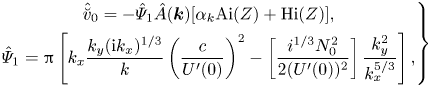 \begin{equation} \left.\begin{gathered} \hat{\breve{v}}_{0}={-}\hat{\varPsi}_{1}\hat{A}(\boldsymbol{k})[\alpha_{k}\mathrm{Ai}(Z)+\mathrm{Hi}(Z)],\\ \hat{\varPsi}_{1}={\rm \pi}\left[k_{x}\frac{k_{y}({\rm i}k_{x})^{1/3}}{k} \left(\frac{c}{U^{\prime}(0)}\right)^{2}-\left[\frac{i^{1/3}N_{0}^{2}}{2(U^{\prime}(0))^{2}}\right] \frac{k_{y}^{2}}{k_{x}^{5/3}}\right], \end{gathered}\right\} \end{equation}
where  $\alpha _{k}$ is a constant specified in (A50a–c) and $\mathrm {Hi}(Z)$ is the Scorer function. This solution incorporates the homogeneous part of the solution $\mathrm {Ai}(Z)$ which is decaying exponentially to zero as $\xi \to \infty$. Similarly to (A45), the ‘inhomogeneous’ contribution is described by the Scorer function $\mathrm {Hi}(Z)$ which decays as $Z^{-1}$ for large values of its complex argument. Thus, when $\xi \to \infty$ the perturbation of streamwise velocity matches the main-deck solution. The same choice of $\alpha _{k}$ in the solution (A53a,b) specified in (A50a–c) ensures that no-stress condition at $\xi =0$ is satisfied for ${\breve {v}}_{0}$ as well.
Matching the derived inner solution of the viscous sub-layer to the outer solution requires 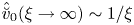 $\hat {\breve {v}}_{0}(\xi \to \infty ) \sim 1/\xi$. To perform this, in the standard manner we first re-write the expression for the main-deck solution in terms of the inner variable $\xi$ using the relation $\xi ={z}/{\delta }$, then substitute it into the expression for $v_{3}$ of the main deck (see (3.41)). By virtue of (A8b)
 \begin{align} {\breve{v}}_{0}(\xi)\to ({\mathcal{R}}-{\mathcal{P}}_{xy})\frac{1}{\xi},\quad {\mathcal{P}} =\left(\frac{U_{max}}{U^{\prime}(0)}\right)^2 \left(f_{Z_{1}}\ast\nabla_{{\perp}}^{{-}2}A\right),\quad {\mathcal{R}}=\frac{N_{0}^{2}}{2(U^{\prime}(0))^{2}}\hat{G}_{3}[A]. \end{align}
Thus, we have derived solution for  $\breve {v}_{0}$ that satisfies both the boundary and matching conditions.
A.4. Uniformly valid solutions inside the viscous sub-layer: summary
Here, we summarize the lengthy analysis of the appendix by providing in one place closed expressions for the uniformly valid solutions. The expressions for the streamwise, spanwise and cross-boundary perturbation velocities satisfying the matching conditions with the outer solutions and no-stress boundary conditions given either in the  $\boldsymbol x$- or Fourier space are
 \begin{equation} \left.\begin{gathered} \breve{w}_{0}=A_{x}\xi,\\ \hat{\breve{w}}_{1}=\frac{\hat{C}}{{\rm Ai}^{\prime}(0)} \left[\xi{\mathcal{I}}-({\rm i}k_{x})^{1/3}{\rm Ai}^{\prime} \left[({\rm i}k_{x})^{1/3}\xi\right]+({\rm i}k_{x})^{1/3}{\rm Ai}^{\prime}(0)- \frac{1}{3({\rm i}k_{x})^{1/3}}\xi\right], \end{gathered}\right\} \end{equation}
where
 \begin{equation} {\mathcal{I}}=\int_{0}^{\xi}{\rm Ai}\left[({\rm i}k_{x})^{1/3}s_{2}\right]\mathrm{d}s_{2}, \end{equation}
and constant 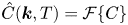 $\hat {C}(\boldsymbol k, T)=\mathcal {F}\{C\}$ is the Fourier transform of $C$. Here, $C$ is specified in the $\boldsymbol x$-space by (A8c)
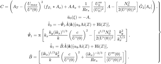 \begin{equation} \left.\begin{gathered} C= \left(A_{T}-\left(\frac{U_{max}}{U^{\prime}(0)}\right)^2 \left(f_{Z_{1}}\ast A_x\right)+AA_x+\frac{1}{Re_{{\ast}}}\left[\frac{U_{0}^{\prime\prime\prime}} {(U_{0}^{\prime})^{2}}\right]A-\left[\frac{N_{0}^{2}}{2(U^{\prime}(0))^{2}}\right] \hat{G}_{2}[A_{x}]\right).\\ \breve{u}_{0}(\xi)={-}A,\\ \hat{\breve{v}}_{0}={-}\hat{\varPsi}_{1}\hat{A}(\boldsymbol{k})[\alpha_{k} \mathrm{Ai}(Z)+\mathrm{Hi}(Z)],\\ \hat{\varPsi}_{1}={\rm \pi}\left[k_{x}\frac{k_{y}({\rm i}k_{x})^{1/3}}{k} \left(\frac{c}{U^{\prime}(0)}\right)^{2}-\left[\frac{i^{1/3}N_{0}^{2}}{2(U^{\prime}(0))^{2}}\right] \frac{k_{y}^{2}}{k_{x}^{5/3}}\right].\\ \hat{\breve{u}}_{1}=\hat{B}\hat{A}(\boldsymbol{k})[\alpha_{k}\mathrm{Ai}(Z)+\mathrm{Hi}(Z)],\\ \hat{B}=\left[\frac{({\rm i}k_{x})^{1/3}k_{y}^{2}}{k} \left(\frac{c}{U^{\prime}(0)}\right)^{2}+\frac{({\rm i}k_{x})^{{-}2/3}}{Re_{{\ast}}} \left[\frac{U^{\prime\prime\prime}(0)}{(U^{\prime}(0))^{2}}\right]\right]. \end{gathered}\right\} \end{equation}
A.5. Conclusions
Thus, we derived the inner solution describing dynamics in the critical layer matched with the main-deck solution. Under the adopted scaling the inner solution represents a forced motion caused by the dynamics in the main deck through the matching conditions. It is expressed as nonlinear functional of amplitude  $A$ – the amplitude of the main-deck perturbation. The uniformly valid expansion (A8a), (A8b), (A8c) we derived describes the motion in the bulk of the boundary layer, while § (A.4) gives the summary of solutions in the critical layer.
Note that, here, we examined the motion in the critical layer from a particular view point: our main aim was to get an uniformly valid asymptotic solution. We showed that its dynamics does not affect motions in the main deck and, hence, the evolution equation obtained by applying the no-flux condition at the surface to the main-deck expansion is correct. However, in other contexts, for example, for detailed comparison with numerics, the derived explicit inner solution might be also of interest per se.


 Open access