


1. Introduction
Wave turbulence theory (WTT) is a statistical closure that provides a coarse-grained description for evolution of random weak wave fields (Zakharov, Lvov & Falkovich Reference Zakharov, Lvov and Falkovich1992; Nazarenko Reference Nazarenko2011; Galtier Reference Galtier2022). It has been applied successfully to very different physical cases, from quantum (Proment, Nazarenko & Onorato Reference Proment, Nazarenko and Onorato2012; Kolmakov, McClintock & Nazarenko Reference Kolmakov, McClintock and Nazarenko2014) to classical (Zakharov & Filonenko Reference Zakharov and Filonenko1967; Zakharov Reference Zakharov1999; Connaughton, Nazarenko & Quinn Reference Connaughton, Nazarenko and Quinn2015) to cosmological (Galtier & Nazarenko Reference Galtier and Nazarenko2017) wave systems. One of the most important applications of WTT is the water surface gravity waves, understanding which is important for sea navigation and industrial offshore activities. A review of important achievements in this area can be found in Nazarenko & Lukaschuk (Reference Nazarenko and Lukaschuk2016). For a kinetic description of weakly nonlinear gravity waves, there are two quadratic (in the wave amplitude) invariants: the energy and the wave action. This system is characterized by a dual cascade behaviour, for which there exist two local Kolmogorov–Zakharov (KZ) spectra, one in which the energy is cascading downscale (Zakharov & Filonenko Reference Zakharov and Filonenko1967), and the other one where the wave action is cascading upscale (Zakharov & Zaslavskii Reference Zakharov and Zaslavskii1982). Realizability of the KZ spectra requires locality of interactions in the scale space, which in turn is possible only if there are sufficiently wide inertial ranges of scales without local energy pile-up in the spectral space. However, often there is no efficient dissipation mechanism at the large scales, which leads to a spectrum pile-up (or condensation) at the scales of the order of the largest available scale in the system – the size of the containing basin. We emphasize that, in contrast with a uniform condensate in an infinite system, our condensate is weakly non-uniform, i.e. it contains small but non-zero wavenumbers. In laboratory experiments and numerical simulations, the largest available scale is limited by the size of the flume or the computational domain, whereas in open seas, this scale may be set by a swell or the water depth. Such condensation can lead to breakdown of locality of interactions.
In the present paper, we will develop a WTT description of gravity waves in the presence of a strong large-scale condensate formed due to inverse cascade. This will allow us to propose an explanation for deviations from the inverse-cascade KZ spectrum that were recently observed numerically in Korotkevich (Reference Korotkevich2023) and earlier reported experimentally in Nazarenko & Lukaschuk (Reference Nazarenko and Lukaschuk2016) and Deike, Laroche & Falcon (Reference Deike, Laroche and Falcon2011).
A standard approach in describing the gravity waves (including that in Korotkevich Reference Korotkevich2023) is to consider a two-dimensional surface over a three-dimensional potential flow of an ideal incompressible infinitely deep fluid with velocity  $\boldsymbol{v} = \boldsymbol{\nabla} \varPhi (x,y,z;t)$, where $\varPhi (x,y,z;t)$ is the velocity potential. Capillary effects are neglected, assuming that they are small with respect to gravity. The Hamiltonian variables for this system are elevation of the surface $\eta (x,y;t)$ and velocity potential on the surface $\psi (x,y;t)=\varPhi (x,y,z;t)|_{z=\eta }$ (Zakharov Reference Zakharov1967). It is convenient to introduce normal canonical variables $a_{\boldsymbol{k}}$, corresponding to expansion in Fourier harmonics as follows:
 \begin{equation} a_{\boldsymbol{k}} = \sqrt \frac{\omega_k}{2k}\,\eta_{\boldsymbol{k}} + \mathrm i\,\sqrt \frac{k}{2\omega_k}\,\psi_{\boldsymbol{k}},\quad \mbox{where } \omega_k = \sqrt {g k}. \end{equation}
In terms of these variables, the surface dynamics is Hamiltonian,
 \begin{equation} \dot a_{\boldsymbol{k}} =-\mathrm i\,\frac{\delta H}{\delta a_{\boldsymbol{k}}^{*}}, \end{equation}
with the Hamiltonian  $H$ being the total physical energy of the wave system (not shown).
For statistical description of a stochastic wave field one can use a pair correlation function called the wave action spectrum,
 \begin{equation} \langle a_{\boldsymbol{k}} a_{\boldsymbol{k}'}^*\rangle = n_{\boldsymbol{k}} \delta (\boldsymbol{k} - \boldsymbol{k}'), \end{equation}
where the angular bracket denotes averaging over the ensemble of initial conditions (which have random phases), and  $\delta$ denotes the Dirac delta function. The spectrum $n_{\boldsymbol{k}}$ is a measurable quantity, directly related to observable correlation functions; e.g. from the definition of $a_{\boldsymbol{k}}$, one can get
 \begin{equation} \langle \eta_{\boldsymbol{k}} \eta_{\boldsymbol{k}'}^*\rangle = I_{\boldsymbol{k}} \delta (\boldsymbol{k} - \boldsymbol{k}') \quad \longrightarrow \quad I_{\boldsymbol{k}} = \frac{1}{2}\,\frac{\omega_k}{g}\,(n_{\boldsymbol{k}} + n_{-\boldsymbol{k}}). \end{equation}
Under the WTT assumptions, i.e. small wave amplitudes, random phases and large-basin limit, spectrum  $n_k$ obeys the Hasselmann wave kinetic equation (WKE) (Nordheim Reference Nordheim1928; Peierls Reference Peierls1929; Hasselmann Reference Hasselmann1962):
 \begin{equation} \frac{\partial n_{\boldsymbol{k}}}{\partial t} = I_{St} + f_p (k) - f_d (k). \end{equation}
Here,  $f_p$ and $f_d$ are some pumping and damping terms respectively, and $I_{St}$ is a so-called collision integral:
 $$\begin{gather} I_{St}=4{\rm \pi} \int \left| T_{\boldsymbol{k},\boldsymbol{k}_1}^{\boldsymbol{k}_2,\boldsymbol{k}_3}\right|^2 n_{\boldsymbol{k}} n_{\boldsymbol{k}_1} n_{\boldsymbol{k}_2} n_{\boldsymbol{k}_3}\left(\frac{1}{n_{\boldsymbol{k}}} + \frac{1}{n_{\boldsymbol{k}_1}} - \frac{1}{n_{\boldsymbol{k}_2}} - \frac{1}{n_{\boldsymbol{k}_3}}\right)\delta (\boldsymbol{k} + \boldsymbol{k}_1- \boldsymbol{k}_2 - \boldsymbol{k}_3)\nonumber\\ {}\times \delta (\omega_k + \omega_{k_1}- \omega_{k_2} - \omega_{k_3}) \,\mathrm{d} \boldsymbol{k}_1\,\mathrm{d} \boldsymbol{k}_2\,\mathrm{d} \boldsymbol{k}_3. \end{gather}$$
The interaction coefficients  $T_{\boldsymbol{k},\boldsymbol{k}_1}^{\boldsymbol{k}_2,\boldsymbol{k}_3}$ can be found in e.g. Pushkarev, Resio & Zakharov (Reference Pushkarev, Resio and Zakharov2003) and in Appendix B. The kinetic equation and its modifications are the basis for all wave forecasting models (Cavaleri et al. Reference Cavaleri2007).
One can consider stationary solutions of the WKE in the so-called inertial interval – range of scales far from pumping and damping regions. Such solutions have to obey the  $I_{St}=0$ equation. Beyond obvious Rayleigh–Jeans thermodynamic equilibrium (zero flux) solutions $n_{\boldsymbol{k}} \sim 1/(\omega _k +{\rm const}$), there are dynamic equilibrium solutions, corresponding to finite fluxes of conserved quantities, the so-called KZ spectra (Zakharov et al. Reference Zakharov, Lvov and Falkovich1992; Nazarenko Reference Nazarenko2011). Equations (1.5)–(1.6) describe a four-wave process of scattering of two waves into two waves. This means that in addition to the total energy $E=\int \omega _k n_{\boldsymbol{k}} \,\mathrm {d}\boldsymbol{k}$, there is a conservation of the total wave action (‘number of waves’) $N=\int n_{\boldsymbol{k}} \,\mathrm {d}\boldsymbol{k}$. Thus there are two KZ spectra: one describing a local downscale (with respect to the forcing scale) energy cascade,
 \begin{equation} n_k^{DC} = C_P P^{1/3} k^{-4}, \end{equation}
and the other one a local upscale (towards smaller  $\boldsymbol{k}$) wave action cascade (Zakharov & Zaslavskii Reference Zakharov and Zaslavskii1982),
 \begin{equation} n_k^{IC} = C_Q Q^{1/3} k^{-23/6}\sim k^{-3.83}. \end{equation}
Here,  $P$ and $Q$ are the fluxes of energy and wave action, respectively, $C_P$ and $C_Q$ are some constants, and $k=|\boldsymbol{k}|$.
In a recent paper Korotkevich (Reference Korotkevich2023), the primordial dynamical equations were simulated in a region  $L_x = L_y = 2{\rm \pi}$ with double periodic boundary conditions, which means that components of $\boldsymbol{k}$'s were integer numbers. Grid resolution was $N_x=N_y=512$. Pumping was isotropic with respect to angle, and concentrated in a ring $k \in (60,64)$ with random phase of every pumped harmonic. Damping started at $k_d=128$. As a result, in the range of wavenumbers smaller than $k=60$, one would expect to find a spectrum similar to (1.8). Nevertheless, it was reported that the observed inverse-cascade spectrum had a different slope, close to $n_k \sim k^{-3.07}$, which was indistinguishable for significantly different levels of nonlinearity in the system. This numerically observed spectrum is rather close to two previous independent experimental results. One of the experiments (Nazarenko & Lukaschuk Reference Nazarenko and Lukaschuk2016), conducted in a tank of size $42\,{\rm cm}\times 42\,{\rm cm}$, showed $n_k \sim k^{-2.5}$ or $n_k \sim k^{-3}$ depending on the forcing frequency (see figure 12 in Nazarenko & Lukaschuk (Reference Nazarenko and Lukaschuk2016) for the corresponding energy spectra $E_k$). The other experiment (Deike et al. Reference Deike, Laroche and Falcon2011), conducted earlier in a $20\,{\rm cm}\times 20\,{\rm cm}$ tank filled with mercury, showed that the spectral slope varies from $n_k \sim k^{-3}$ to $n_k \sim k^{-3.65}$ (see figure 2 in Deike et al. (Reference Deike, Laroche and Falcon2011) for the corresponding frequency spectrum $E_\omega$), from low to high nonlinearity levels. In particular, the $k^{-3}$ spectrum at low nonlinearity is associated with a clear condensate at large scales, whereas the $k^{-3.65}$ spectrum (closer to the KZ solution) is present without a clear condensate, perhaps due to some effective large-scale dissipation mechanism at high nonlinearity in their experiment, e.g. bottom or/and wall friction.
In previous works (Korotkevich Reference Korotkevich2008, Reference Korotkevich2012), it was shown that condensate plays an important role in the nonlinear interaction processes for such systems. Specifically, the measured dispersion relation in Korotkevich (Reference Korotkevich2013) demonstrated that the influence of the condensate on the harmonics in the region of inverse cascade cannot be neglected. There are several approaches that allow one to take the condensate influence into account. Probably the most obvious one is based on Bogolyubov's transformation technique, as in the case of dilute Bose gas, similar to the recent work in Griffin et al. (Reference Griffin, Krstulovic, L'vov and Nazarenko2022) – see sections about degenerated almost ideal Bose gas in Abrikosov, Gorkov & Dzyaloshinskii (Reference Abrikosov, Gorkov and Dzyaloshinskii1962) or Lifshitz & Pitaevskii (Reference Lifshitz and Pitaevskii1978). This approach requires the condensate to be a coherent object, which is usually achieved due to the fact that it is located at a single harmonic,  $k=0$. In the case of numerical simulations in Korotkevich (Reference Korotkevich2023), the condensate was roughly a ring in the $k$-space, whose further cascade to low wavenumbers is prohibited by the finite size effect of the domain. The pictures of the $|a_{\boldsymbol{k}}|^2$ distributions are shown in figure 1.

Figure 1. Surfaces of  $|a_{\boldsymbol{k}}|^2\times 10^{8}$ in the condensate region for four simulations of Korotkevich (Reference Korotkevich2023) corresponding to four different mean wave slopes $\mu$, for (a) $\mu = 0.054$, (b) $\mu = 0.067$, (c) $\mu = 0.093$, (d) $\mu = 0.135$.
One can see that the wave amplitudes are randomized and, in most cases, are significantly different from each other in amplitude even for harmonics close in  ${\bf k}$. So the Bogolyubov approach is clearly not applicable. There are more than a hundred harmonics in the condensate ring. Since averaging over an ensemble of realizations is computationally unfeasible, we average the $|a_{\boldsymbol{k}}|^2$ function over the azimuthal angle, and obtain an object $\langle |a_{\boldsymbol{k}}|^2\rangle$, which can be considered as an approximation for $n_k$. Thus one can try to modify the WKE (1.5) to describe the statistics of the wave field on the background of condensate.
In the remainder of the paper, we will describe our new theoretical development following the above idea that allows an explanation of the  $k^{-3}$ spectrum observed in experiments and simulations. There are two major elements of our development. First, there is the derivation of a spectral diffusion equation for surface gravity waves in the presence of condensate. In addition to the derivation from the WKE that we have in the main paper, we also put an alternative derivation in Appendix C, which relies on a Wentzel–Kramers–Brillouin (WKB) approximation of the Zakharov equation. The two approaches yield exactly the same result, including the detailed formulation of the diffusion coefficient. We note that the spectral diffusion equation has been developed previously for triad-resonant systems, such as internal gravity waves (McComas & Bretherton Reference McComas and Bretherton1977), Rossby waves (Connaughton et al. Reference Connaughton, Nazarenko and Quinn2015) and magnetohydrodynamic (MHD) turbulence (Nazarenko, Newell & Galtier Reference Nazarenko, Newell and Galtier2001). Our current work provides the first systematic formulation for a quartet-resonant system, which involves much more complexity in both approaches of derivation. The second element is a careful analysis on the asymptotics of the interaction coefficient at the limit of non-local interactions. We will show that this calculation yields a remarkable cancellation of all leading-order terms, which is crucial in obtaining the correct scaling of the diffusion coefficient. Finally, it is the combination of these two elements that allows us to achieve the correct stationary solution with the $k^{-3}$ spectrum.
2. New theory on non-local gravity wave turbulence
2.1. Derivation of the diffusion equation in the presence of condensate
Assume that the condensate modes are much stronger than any other harmonics, so that for any four waves in the resonant quartet, the dominant contribution comes from the situation that two waves  $\boldsymbol{k}_1$ and
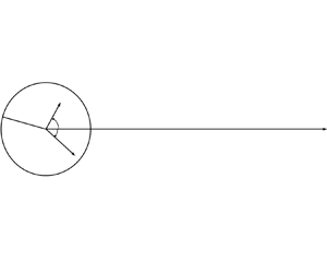
  $\boldsymbol{k}_3$ are in the condensate (see figure 2), satisfying
 \begin{equation} \boldsymbol{k} + \boldsymbol{k}_1 = \boldsymbol{k}_2 + \boldsymbol{k}_3,\quad \omega_k + \omega_{k_1} = \omega_{k_2} + \omega_{k_3}. \end{equation}
We consider the case  $k\gg k_{1,3}$ and strong condensate $n_{\boldsymbol{k}_{1,3}}\gg n_{\boldsymbol{k}}, n_{\boldsymbol{k}_2}$. The case when both condensate waves are at one side of resonant conditions (2.1a,b) cannot be realized. The situation is isotropic with respect to azimuthal angle. For simplicity, let us consider the case where the condensate is supported in a ring as in figure 2. Writing $\boldsymbol{q} = \boldsymbol{k}_1 - \boldsymbol{k}_3$ for the difference of wave vectors, i.e. $\boldsymbol{k}_2 = \boldsymbol{k} + \boldsymbol{q}$, and neglecting $1/n_{\boldsymbol{k}_{1,3}}$ terms in (1.6), one gets
 \begin{equation} \frac{\partial n_{\boldsymbol{k}}}{\partial t} \approx 8{\rm \pi} \int \left\{\left| T_{\boldsymbol{k},\boldsymbol{k}_1}^{\boldsymbol{k}_2,\boldsymbol{k}_3}\right|^2 n_{\boldsymbol{k}_1} n_{\boldsymbol{k}_3}( n_{\boldsymbol{k}_2} - n_{\boldsymbol{k}}) \displaystyle \delta (\varOmega)\right\}_{\boldsymbol{k}_2 = \boldsymbol{k}+\boldsymbol{q}} \,\mathrm{d} \boldsymbol{k}_1\,\mathrm{d} \boldsymbol{k}_3, \end{equation}
where  $\varOmega = \omega _k + \omega _{k_1}- \omega _{k_2} - \omega _{k_3}$. The additional factor of two relative to (1.6) is due to the fact that the condensate is supported on either $\boldsymbol{k}_2$ or $\boldsymbol{k}_3$.

Figure 2. Scheme of considered wave vectors with respect to position of condensate ring.
Next, we exploit Taylor expansion in  $\boldsymbol{q}$ of the expression
 \begin{equation} \left|T_{\boldsymbol{k},\boldsymbol{k}_1}^{\boldsymbol{k}_2,\boldsymbol{k}_3}\right|^2( n_{\boldsymbol{k}_2} - n_{\boldsymbol{k}}), \end{equation}
where  $\boldsymbol{k}_2= \boldsymbol{k} + \boldsymbol{q}$ to second order (see Appendix A):
 \begin{align} \frac{\partial n_{\boldsymbol{k}}}{\partial t} &\approx 8{\rm \pi} \int n_{\boldsymbol{k}_1} n_{\boldsymbol{k}_3} \left|T_{\boldsymbol{k},\boldsymbol{k}_1}^{\boldsymbol{k}, \boldsymbol{k}_3}\right|^2\boldsymbol{q}\boldsymbol{\cdot}\boldsymbol{\nabla}_{\boldsymbol{k}}n_{\boldsymbol{k}} \left.\delta (\varOmega)\right|_{\boldsymbol{k}_2 = \boldsymbol{k}+\boldsymbol{q}} \,\mathrm{d} \boldsymbol{k}_1\,\mathrm{d} \boldsymbol{k}_3\nonumber\\ &\quad +4{\rm \pi}\int n_{\boldsymbol{k}_1} n_{\boldsymbol{k}_3} \left\{ 2\left.\left(\boldsymbol{q}\boldsymbol{\cdot}\boldsymbol{\nabla}_{\boldsymbol{k}_2}\left|T_{\boldsymbol{k},\boldsymbol{k}_1}^{\boldsymbol{k}_2, \boldsymbol{k}_3}\right|^2\right)\right|_{\boldsymbol{k}_2 =\boldsymbol{k}}\boldsymbol{q}\boldsymbol{\cdot}\boldsymbol{\nabla}_{\boldsymbol{k}}n_{\boldsymbol{k}} \right.\nonumber\\ &\quad+ \left.\left|T_{\boldsymbol{k},\boldsymbol{k}_1}^{\boldsymbol{k}, \boldsymbol{k}_3}\right|^2\boldsymbol{q}\boldsymbol{\cdot}\boldsymbol{\nabla}_{\boldsymbol{k}}\left(\boldsymbol{q}\boldsymbol{\cdot}\boldsymbol{\nabla}_{\boldsymbol{k}}n_{\boldsymbol{k}}\right) \right\}\left.\delta (\varOmega)\right|_{\boldsymbol{k}_2 = \boldsymbol{k}+\boldsymbol{q}} \,\mathrm{d} \boldsymbol{k}_1\,\mathrm{d} \boldsymbol{k}_3. \end{align}
 To simplify (2.4), we consider the expansion of  $\varOmega$ in $\boldsymbol{q}$:
 \begin{equation} \varOmega = \omega_{k_1} -\omega_{k_3} -\boldsymbol{\nabla}_{\boldsymbol{k}}\omega_k\boldsymbol{\cdot} \boldsymbol{q} + O(|\boldsymbol{q}|^2). \end{equation}
Using the equation  $\omega _k= \sqrt {gk}$, we obtain
 \begin{align} \varOmega &\approx \omega_{k_1}-\omega_{k_3} -\frac{\sqrt{g}}{2}\,\frac{\boldsymbol{k}}{k^{3/2}}\boldsymbol{\cdot}(\boldsymbol{k}_1- \boldsymbol{k}_3)\nonumber\\ &= \omega_{k_1}-\omega_{k_3} -\frac{\sqrt{g}}{2}\,\frac{k_1\cos\alpha - k_3\cos\beta}{k^{1/2}}, \end{align}
where  $\alpha$ and $\beta$ are as in figure 2. Here, we keep the next order term, which becomes part of the leading one if $k_1\approx k_3$. It should be noted that $\delta (\varOmega )$ (here and below we use the last expression for $\varOmega$) is invariant with respect to exchange $\boldsymbol{k}_1\leftrightarrow \boldsymbol{k}_3$. Using this symmetry as well as $T_{\boldsymbol{k},\boldsymbol{k}_1}^{\boldsymbol{k}_2, \boldsymbol{k}_3}=T_{\boldsymbol{k}_2,\boldsymbol{k}_3}^{\boldsymbol{k}, \boldsymbol{k}_1}$, and taking into account the fact that $\boldsymbol{k}_1$ and $\boldsymbol{k}_3$ are dummy variables so that value of an integral must not change after exchange $\boldsymbol{k}_1 \leftrightarrow \boldsymbol{k}_3$, the first term of (2.4) is integrated to zero, due to change of sign of $\boldsymbol{q}$ after the mentioned exchange of integration variables. For evaluation of the second term in (2.4) at $\boldsymbol{k}_2=\boldsymbol{k}$, one can use
 \begin{equation} \left.\boldsymbol{\nabla}_{\boldsymbol{k}_2}\left|T_{\boldsymbol{k},\boldsymbol{k}_1}^{\boldsymbol{k}_2, \boldsymbol{k}_3}\right|^2\right|_{\boldsymbol{k}_2 =\boldsymbol{k}} = \left.\boldsymbol{\nabla}_{\boldsymbol{k}}\left|T_{\boldsymbol{k}_2,\boldsymbol{k}_1}^{\boldsymbol{k}, \boldsymbol{k}_3}\right|^2\right|_{\boldsymbol{k}_2 =\boldsymbol{k}} = \frac{1}{2}\,\boldsymbol{\nabla}_{\boldsymbol{k}}\left|T_{\boldsymbol{k},\boldsymbol{k}_1}^{\boldsymbol{k}, \boldsymbol{k}_3}\right|^2, \end{equation}
where the second equality should be understood in the context of integration over  $\boldsymbol{k}_1$ and $\boldsymbol{k}_3$ as in (2.4). As a result, (2.4) can be transformed (after combining the second and third terms) into the expression
 \begin{equation} \frac{\partial n_{\boldsymbol{k}}}{\partial t} \approx 4{\rm \pi}\int n_{\boldsymbol{k}_1} n_{\boldsymbol{k}_3} \boldsymbol{\nabla}_{\boldsymbol{k}}\boldsymbol{\cdot} \left(\boldsymbol{q} \left|T_{\boldsymbol{k},\boldsymbol{k}_1}^{\boldsymbol{k}, \boldsymbol{k}_3}\right|^2\boldsymbol{q}\boldsymbol{\cdot} \boldsymbol{\nabla}_{\boldsymbol{k}}n_{\boldsymbol{k}}\right) \displaystyle \delta (\varOmega) \,\mathrm{d} \boldsymbol{k}_1\,\mathrm{d} \boldsymbol{k}_3 . \end{equation}
This is a continuity equation for the wave action  $n_{\boldsymbol{k}}$,
 \begin{equation} \frac{\partial n_{\boldsymbol{k}}}{\partial t} + \boldsymbol{\nabla}_{\boldsymbol{k}} \boldsymbol{\cdot} \boldsymbol{Q}_{\boldsymbol{k}}=0 \end{equation}
with action flux  $\boldsymbol{Q}_{\boldsymbol{k}}$ for an isotropic spectrum, where
 \begin{equation} \boldsymbol{Q}_{\boldsymbol{k}} =- 4{\rm \pi} \int n_{\boldsymbol{k}_1}n_{\boldsymbol{k}_3} \boldsymbol{q} \left| T_{\boldsymbol{k},\boldsymbol{k}_1}^{\boldsymbol{k},\boldsymbol{k}_3}\right|^2 \frac{\boldsymbol{q}\boldsymbol{\cdot}\boldsymbol{k}}{k}\,\frac{\partial n_{k}}{\partial k}\,\delta (\varOmega) \,\mathrm{d} \boldsymbol{k}_1\,\mathrm{d} \boldsymbol{k}_3. \end{equation}
Under the same isotropic consideration, we have
 $$\begin{gather} N=\int n_{\boldsymbol{k}}\,\mathrm{d}\boldsymbol{k} =\int n_{k} 2{\rm \pi} k\,\mathrm{d} k, \end{gather}$$
 $$\begin{gather}\frac{\partial (2{\rm \pi} k n_k)}{\partial t} +\frac{\partial Q_{ k}}{\partial k}=0. \end{gather}$$
Here, we introduced the isotropic wave action flux
 \begin{align} Q_k &=2{\rm \pi}\boldsymbol{k} \boldsymbol{\cdot}\boldsymbol{Q}_{\boldsymbol{k}}=-\left[\frac {8{\rm \pi}^2} k \int n_{\boldsymbol{k}_1}n_{\boldsymbol{k}_3}\, \delta (\varOmega) \right.\nonumber\\ &\quad \left.{}\times\left(\left| T_{\boldsymbol{k},\boldsymbol{k}_1}^{\boldsymbol{k},\boldsymbol{k}_3}\right|^2 (\boldsymbol{q} \boldsymbol{\cdot}\boldsymbol{k})^2 \right) \,\mathrm{d} \boldsymbol{k}_1\,\mathrm{d} \boldsymbol{k}_3\right]\frac{\partial n_{k}}{\partial k}. \end{align}
One can integrate out  $k_3$ using $\delta (\varOmega )$. In order to do this, we need to set $\varOmega =0$ in (2.6). Solving this quadratic equation for $\sqrt {k_3}$ and taking into account condition $k_1\ll k$, we get
 \begin{equation} k_3 \approx k_1 -k_1\sqrt{\frac{k_1}{k}}\,(\cos\alpha-\cos\beta). \end{equation}
The integration in (2.13) is over  $0\le \alpha,\beta <2{\rm \pi}$ and $k_1$. If the relative width of the condensate ring $\varepsilon /k_0$ is small, then from (2.14), $k_3$ will be outside the ring for various values of $\alpha, \beta \in (0,2{\rm \pi} )$; see figure 2. However, if the condensate ring is wide ( $\varepsilon /k_0 \gg 2 (k_0/k)^{1/2}$), then we can always find $k_3 \approx k_1$ for all $0\le \alpha,\beta <2{\rm \pi}$. In other words, in the non-local resonant quartets, the lengths of vectors $\boldsymbol{k}_1$ and $\boldsymbol{k}_3$ are nearly equal, whereas their respective directions are allowed to be arbitrary (details can be found in Appendix D). As a result of the above strong inequality, we can take $n_{k_3}=n_{k_1}$, thus we have a diffusion equation
 \begin{equation} 2{\rm \pi} k\,\frac{\partial n_{k}}{\partial t} = \frac{\partial}{\partial k} \left(D_k\,\frac{\partial n_{k}}{\partial k} \right), \end{equation}
with diffusion coefficient
 \begin{equation} D_k = 8{\rm \pi}^2 k \int_{k_1 \ll k}n_{k_1}^2\,\frac{k_1^4}{\left|\dfrac{{\rm d} \omega_{k_1}}{{\rm d} k_1}\right|}\left[\int_{0}^{2{\rm \pi}} \int_{0}^{2{\rm \pi}} \left| T_{\boldsymbol{k},\boldsymbol{k}_1}^{\boldsymbol{k},\boldsymbol{k}_3}\right|^2 (\cos\beta-\cos\alpha)^2 \,\mathrm{d}\alpha\,\mathrm{d} \beta\right]\mathrm{d} k_1. \end{equation}
2.2. Asymptotics of the interaction coefficient and stationary solution
In Appendix B, it is shown that the first non-vanishing term in the expansion of  $T_{\boldsymbol{k},\boldsymbol{k}_1}^{\boldsymbol{k},\boldsymbol{k}_3}$ in $k_{1,3}/k$ (after cancellation of all leading-order terms of order $k^2k_1$) is
 \begin{equation} T_{\boldsymbol{k},\boldsymbol{k}_1}^{\boldsymbol{k},\boldsymbol{k}_3}=-\frac{(k k_1)^{3/2}}{16{\rm \pi}^2}\,(\cos\alpha -\cos\beta)^2. \end{equation}
To find the diffusion coefficient (2.16), one needs to compute the following integral using (2.17):
 \begin{equation} \int_{0}^{2{\rm \pi}}\int_{0}^{2{\rm \pi}} \left| T_{\boldsymbol{k},\boldsymbol{k}_1}^{\boldsymbol{k},\boldsymbol{k}_3}\right|^2 (\cos\beta-\cos\alpha)^2 \,\mathrm{d}\alpha\,\mathrm{d} \beta = \frac{25(k k_1)^{3}}{256{\rm \pi}^2}, \end{equation}
which results in
 \begin{equation} D_k =\lambda k^4, \quad \lambda = \frac{25{\rm \pi}}{16} \int_{k_1 \ll k}n_{k_1}^2 k_1^{15/2} \,\mathrm{d} k_1 = \text{const}. \end{equation}
Note that we lose the universal (i.e. independent of the spectrum shape) scaling  $D_k \sim k^4$ if the width of the condensate is $\varepsilon /k_0 \sim (k_0/k)^{1/2}$.
Note also that the expression for the diffusion coefficient (2.19) is different from the one previously obtained in Zakharov (Reference Zakharov2010), which is a consequence of an error in obtaining the asymptotics of the interaction coefficient made in the latter paper. The calculation of the latter paper is for a different purpose of obtaining the locality window of power-law spectra of gravity waves. As a result, we can now correct the upper boundary of locality for the power-law spectra  $n_k \sim k^{-x}$, which follows from the convergence condition in the integral of (2.19), giving $x<17/4$ (cf. the respective condition $x<19/4$ written in Zakharov Reference Zakharov2010). This correction makes the locality window narrower than previously thought, but does not affect the forward and inverse-cascade KZ spectra as local solutions (just by the margin of $1/4$ in the forward cascade!). The correction in (2.19) also likely affects the lower boundary of the locality window according to the procedure outlined in Zakharov (Reference Zakharov2010). However, the calculation for the UV boundary is much more involved, and the procedure needs to be put under close scrutiny before a definitive answer can be given. We leave this task to our future work.
From  $Q=-D_k\,\partial n_{k}/\partial k = {\rm const}$, we immediately get
 \begin{equation} n_{k} = \frac{Q}{3\lambda}\,k^{-3}, \end{equation}
which is a constant-flux power-law solution. Note that since both  $n_{k}$ and $\lambda$ are positive, the wave action flux $Q$ is positive too, i.e. it is towards high $k$ and has the opposite direction with respect to the wave action flux on the local KZ solution with $Q={\rm const}$. But by the standard Fjortoft argument, the wave action cannot be continuously transferred to high $k'$ values – otherwise, the amount of energy transferred to these wavenumbers would be greater than the energy produced by the forcing, which is impossible. Therefore, the non-local cascade must drain energy from the condensate. Indeed, for the energy of the out-of-condensate modes, we have from (2.15) that
 \begin{equation} \dot E= \int \omega_k (D_k n_k')' \,{\rm d}k = \frac{7\lambda}{4} \int k^{5/2} n_k \,{\rm d}k >0. \end{equation}
Thus for any shape of  $n_k$, the energy of the out-of-condensate modes is growing, and since the total energy must be conserved, in the absence of forcing and dissipation, we conclude that the condensate energy must be decreasing at the same rate. We also conclude that for a steady state to exist, there should exist a mechanism of supplying the energy from the forcing region to the condensate that is not the diffusive mechanism arising from the WKE in the non-local regime (since the latter transfers energy in the opposite direction).
3. Conclusions and discussion
In this paper, we considered turbulence of water surface gravity waves and developed a WTT for non-local wave action spectrum evolution in the presence of a strong large-scale condensate. We derived a singular inhomogeneous spectral diffusion equation governing such an evolution. We found a stationary solution corresponding to a constant wave action cascade,  $n_{k}\sim k^{-3}$, and proposed it as an explanation of the spectrum observed numerically in Korotkevich (Reference Korotkevich2023) and experimentally in recent wave tank experiments (Nazarenko & Lukaschuk Reference Nazarenko and Lukaschuk2016; Deike et al. Reference Deike, Laroche and Falcon2011).
Regarding the mechanism of supply of energy and wave action to the condensate, one can envisage two scenarios. First, the condensate could be built up via a local inverse cascade at the initial stages, followed by the non-local regime switching the cascade direction. Clearly, in this case the non-local regime would not be able to sustain itself due to the condensate drainage (the existence of a stationary solution in the absence of a large-scale forcing is prohibited by the wave action conservation), and the system would return to the local regime with a possible periodic repetition of the local–non-local cycle. We rule out this possibility because no such oscillations are observed in the numerical simulations. The second possibility is excitation of the condensate modes directly from a non-resonant three-wave process following modulational instability of the forcing modes. Such a mechanism requires that the spectrum of the waves in the forcing range is sufficiently strong – clearly, a feature seen in the numerical results of Korotkevich (Reference Korotkevich2023). Moreover, the latter process could remain active simultaneously with the non-local direct cascade and thereby contribute to formation of a stationary spectrum. However, this scenario, proposing an implicit forcing mechanism, which could possibly explain the existence of the steady non-local cascade in the numerics of Korotkevich (Reference Korotkevich2023), remains speculative and requires further validation.
In this paper, we mostly considered the effect of the resonant wave quartets, which implies that all the scales, including the condensate, are populated by weakly nonlinear waves. However, the WKB description (C20) derived in Appendix C does include the non-resonant non-local interactions; it is valid for the cases when the condensate scales are strongly nonlinear. Making analytical predictions about the spectra in this case is difficult as it implies knowledge of the low- $k$ dynamics, which is not a part of the WKB description itself. This can be done in future by assuming a simplified model for the low-k dynamics or by using direct numerical simulations for resolving the low wavenumber part, and using a ‘particle-in-cell method’ for the high-frequency WKB equations, as done previously for acoustic waves in Nazarenko, Zabusky & Scheidegger (Reference Nazarenko, Zabusky and Scheidegger1995).
Acknowledgements
This work was completed when Alexander Korotkevich was a professor at the University of New Mexico. The author's present addresses are: Center for Engineering Physics, Skolkovo Institute of Science and Technology, Bolshoy Boulevard, 30, p. 1, Moscow, 121205 Russia; Landau Institute for Theoretical Physics, Academician Semenov Prospekt, 1a, Chernogolovka, Moscow region, 142432 Russia.
Funding
The authors are grateful for support from the Simons’ Collaboration on Wave Turbulence (award no. 651459). The research was partially performed during a visit of A.O.K. to the Université Côte d'Azur/Institut de Physique de Nice, France, funded by the Fédération de Recherche ‘Wolfgang Döblin’ and the ‘Waves Complexity’ visiting researcher programme, and visits of A.O.K., S.V.N. and Y.P. to the Courant Institute.
Declaration of interests
The authors report no conflict of interest.
Appendix A. Taylor expansion of an integrand up to second order
Let us start from the  $\boldsymbol{k}$ and $\boldsymbol{k}_2$ dependent part of an integrand. We will also use the fact that $\boldsymbol{k}_1$ and $\boldsymbol{k}_3$ are dummy variables (used for integration), and can be exchanged with proper adjustment of an integrand without the change of the value of the integral. We will consider Taylor expansion of the expression
 \begin{equation} F=\left|T_{\boldsymbol{k},\boldsymbol{k}_1}^{\boldsymbol{k}_2, \boldsymbol{k}_3}\right|^2(n_{\boldsymbol{k}_2} - n_{\boldsymbol{k}}) \end{equation}
with respect to  $\boldsymbol{k}_2 = \boldsymbol{k} + \boldsymbol{q}$ around $\boldsymbol{k}$; here, $\boldsymbol{q} = \boldsymbol{k}_1 - \boldsymbol{k}_3$. It should be noted that $T_{\boldsymbol{k},\boldsymbol{k}_1}^{\boldsymbol{k}_2, \boldsymbol{k}_3}$ is a homogeneous function, so one could divide all $\boldsymbol{k}_i$ by $k$ and use the fact that we consider the setting where $k_{1,3}/k\ll 1$, so $|\boldsymbol{q}|/k\ll 1$, and expansion of $T_{\boldsymbol{k},\boldsymbol{k}_1}^{\boldsymbol{k}_2, \boldsymbol{k}_3}$ considering $|\boldsymbol{q}|$ small with respect to $k$ is a valid procedure. Also we suppose that function $n_{\boldsymbol{k}}$ has all necessary properties, so it can be expanded in terms of $\boldsymbol{q}$ considering it as a small perturbation. For instance, numerical data in Korotkevich (Reference Korotkevich2023) supposed $n_{k}\sim k^{-3.07}$, which is a decaying power-law function that again allows us to divide all $\boldsymbol{k}_i$ by $k$, so again Taylor expansion assuming $|\boldsymbol{q}|$ small with respect to $k$ is a reasonable procedure.
The zeroth order of the expansion is obviously zero:
 \begin{equation} F|_{\boldsymbol{k}_2 =\boldsymbol{k}} = 0. \end{equation}
The first order of the expansion is (before evaluation at  $\boldsymbol{k}_2=\boldsymbol{k}$)
 \begin{equation} D_{\boldsymbol{k}_2} F = \left(\boldsymbol{q}\boldsymbol{\cdot}\boldsymbol{\nabla}_{\boldsymbol{k}_2}\left|T_{\boldsymbol{k},\boldsymbol{k}_1}^{\boldsymbol{k}_2, \boldsymbol{k}_3}\right|^2\right)(n_{\boldsymbol{k}_2} - n_{\boldsymbol{k}}) + \left|T_{\boldsymbol{k},\boldsymbol{k}_1}^{\boldsymbol{k}_2, \boldsymbol{k}_3}\right|^2\boldsymbol{q}\boldsymbol{\cdot}\boldsymbol{\nabla}_{\boldsymbol{k}_2}n_{\boldsymbol{k}_2}. \end{equation}
Evaluated at  $\boldsymbol{k}_2 =\boldsymbol{k}$, this expression is
 \begin{equation} \left.D_{\boldsymbol{k}_2} F\right|_{\boldsymbol{k}_2 =\boldsymbol{k}} = \left|T_{\boldsymbol{k},\boldsymbol{k}_1}^{\boldsymbol{k}, \boldsymbol{k}_3}\right|^2\boldsymbol{q}\boldsymbol{\cdot}\boldsymbol{\nabla}_{\boldsymbol{k}}n_{\boldsymbol{k}}. \end{equation}
Using the symmetry  $T_{\boldsymbol{k},\boldsymbol{k}_1}^{\boldsymbol{k}_2, \boldsymbol{k}_3}=T_{\boldsymbol{k}_2,\boldsymbol{k}_3}^{\boldsymbol{k}, \boldsymbol{k}_1}$ and taking into account the already mentioned fact that $\boldsymbol{k}_1$ and $\boldsymbol{k}_3$ are dummy variables, and the value of an integral must not change after exchange $\boldsymbol{k}_1 \leftrightarrow \boldsymbol{k}_3$, this expression will be integrated to zero, because the integral of (A4) changes sign due to change of sign of $\boldsymbol{q}$ after the mentioned exchange of integration variables. So one needs to consider the next order of the expansion.
Using (A3), the second order of the expansion is (before evaluation at  $\boldsymbol{k}_2=\boldsymbol{k}$)
 \begin{align} D_{\boldsymbol{k}_2}^2 F &= D_{\boldsymbol{k}_2}(D_{\boldsymbol{k}_2} F) = \boldsymbol{q}\boldsymbol{\cdot}\boldsymbol{\nabla}_{\boldsymbol{k}_2}\left(\boldsymbol{q}\boldsymbol{\cdot}\boldsymbol{\nabla}_{\boldsymbol{k}_2}\left|T_{\boldsymbol{k},\boldsymbol{k}_1}^{\boldsymbol{k}_2, \boldsymbol{k}_3}\right|^2\right)(n_{\boldsymbol{k}_2} - n_{\boldsymbol{k}}) + \left(\boldsymbol{q}\boldsymbol{\cdot}\boldsymbol{\nabla}_{\boldsymbol{k}_2}\left|T_{\boldsymbol{k},\boldsymbol{k}_1}^{\boldsymbol{k}_2, \boldsymbol{k}_3}\right|^2\right)\boldsymbol{q}\boldsymbol{\cdot}\boldsymbol{\nabla}_{\boldsymbol{k}_2}n_{\boldsymbol{k}_2} \nonumber\\ &\quad +\left(\boldsymbol{q}\boldsymbol{\cdot}\boldsymbol{\nabla}_{\boldsymbol{k}_2}\left|T_{\boldsymbol{k},\boldsymbol{k}_1}^{\boldsymbol{k}_2, \boldsymbol{k}_3}\right|^2\right)\boldsymbol{q}\boldsymbol{\cdot}\boldsymbol{\nabla}_{\boldsymbol{k}_2}n_{\boldsymbol{k}_2} + |T_{\boldsymbol{k},\boldsymbol{k}_1}^{\boldsymbol{k}_2, \boldsymbol{k}_3}|^2\boldsymbol{q}\boldsymbol{\cdot}\boldsymbol{\nabla}_{\boldsymbol{k}_2}\left(\boldsymbol{q}\boldsymbol{\cdot}\boldsymbol{\nabla}_{\boldsymbol{k}_2}n_{\boldsymbol{k}_2}\right)\nonumber\\ &=\boldsymbol{q}\boldsymbol{\cdot}\boldsymbol{\nabla}_{\boldsymbol{k}_2}\left(\boldsymbol{q}\boldsymbol{\cdot}\boldsymbol{\nabla}_{\boldsymbol{k}_2}\left|T_{\boldsymbol{k},\boldsymbol{k}_1}^{\boldsymbol{k}_2, \boldsymbol{k}_3}\right|^2\right)(n_{\boldsymbol{k}_2} - n_{\boldsymbol{k}}) \nonumber\\ &\quad + 2\left(\boldsymbol{q}\boldsymbol{\cdot}\boldsymbol{\nabla}_{\boldsymbol{k}_2}\left|T_{\boldsymbol{k},\boldsymbol{k}_1}^{\boldsymbol{k}_2, \boldsymbol{k}_3}\right|^2\right)\boldsymbol{q}\boldsymbol{\cdot}\boldsymbol{\nabla}_{\boldsymbol{k}_2}n_{\boldsymbol{k}_2} + \left|T_{\boldsymbol{k},\boldsymbol{k}_1}^{\boldsymbol{k}_2, \boldsymbol{k}_3}\right|^2\boldsymbol{q}\boldsymbol{\cdot}\boldsymbol{\nabla}_{\boldsymbol{k}_2}\left(\boldsymbol{q}\boldsymbol{\cdot}\boldsymbol{\nabla}_{\boldsymbol{k}_2}n_{\boldsymbol{k}_2}\right). \end{align}
Evaluating (A5) at  $\boldsymbol{k}_2=\boldsymbol{k}$, one gets
 \begin{equation} \left.D_{\boldsymbol{k}_2}^2 F\right|_{\boldsymbol{k}_2 =\boldsymbol{k}} = 2\left.\left(\boldsymbol{q}\boldsymbol{\cdot}\boldsymbol{\nabla}_{\boldsymbol{k}_2}\left|T_{\boldsymbol{k},\boldsymbol{k}_1}^{\boldsymbol{k}_2, \boldsymbol{k}_3}\right|^2\right)\right|_{\boldsymbol{k}_2 =\boldsymbol{k}}\boldsymbol{q}\boldsymbol{\cdot}\boldsymbol{\nabla}_{\boldsymbol{k}}n_{\boldsymbol{k}} + \left|T_{\boldsymbol{k},\boldsymbol{k}_1}^{\boldsymbol{k}, \boldsymbol{k}_3}\right|^2\boldsymbol{q}\boldsymbol{\cdot}\boldsymbol{\nabla}_{\boldsymbol{k}}\left(\boldsymbol{q}\boldsymbol{\cdot}\boldsymbol{\nabla}_{\boldsymbol{k}}n_{\boldsymbol{k}}\right).\end{equation}
Using again the symmetry  $T_{\boldsymbol{k},\boldsymbol{k}_1}^{\boldsymbol{k}_2, \boldsymbol{k}_3}=T_{\boldsymbol{k}_2,\boldsymbol{k}_3}^{\boldsymbol{k}, \boldsymbol{k}_1}$ and the fact that every term in (A6) has two factors $\boldsymbol{q}$, so exchange $\boldsymbol{k}_1 \leftrightarrow \boldsymbol{k}_3$ does not change the signs of terms, for evaluation of the first term of (A6) at $\boldsymbol{k}_2=\boldsymbol{k}$ one can use the equality
 \begin{equation} \left.\boldsymbol{\nabla}_{\boldsymbol{k}_2}\left|T_{\boldsymbol{k},\boldsymbol{k}_1}^{\boldsymbol{k}_2, \boldsymbol{k}_3}\right|^2\right|_{\boldsymbol{k}_2 =\boldsymbol{k}} = \left.\boldsymbol{\nabla}_{\boldsymbol{k}}\left|T_{\boldsymbol{k}_2,\boldsymbol{k}_1}^{\boldsymbol{k}, \boldsymbol{k}_3}\right|^2\right|_{\boldsymbol{k}_2 =\boldsymbol{k}} = \frac{1}{2}\,\boldsymbol{\nabla}_{\boldsymbol{k}}\left|T_{\boldsymbol{k},\boldsymbol{k}_1}^{\boldsymbol{k}, \boldsymbol{k}_3}\right|^2. \end{equation}
As a result, we get the following expansion of  $F$ up to second order:
 \begin{align} F&=\left|T_{\boldsymbol{k},\boldsymbol{k}_1}^{\boldsymbol{k}_2, \boldsymbol{k}_3}\right|^2(n_{\boldsymbol{k}_2} - n_{\boldsymbol{k}})\approx \left(\boldsymbol{q}\boldsymbol{\cdot}\boldsymbol{\nabla}_{\boldsymbol{k}}\left|T_{\boldsymbol{k},\boldsymbol{k}_1}^{\boldsymbol{k}, \boldsymbol{k}_3}\right|^2\right)\boldsymbol{q}\boldsymbol{\cdot}\boldsymbol{\nabla}_{\boldsymbol{k}}n_{\boldsymbol{k}} + \left|T_{\boldsymbol{k},\boldsymbol{k}_1}^{\boldsymbol{k}, \boldsymbol{k}_3}\right|^2\boldsymbol{q}\boldsymbol{\cdot}\boldsymbol{\nabla}_{\boldsymbol{k}}\left(\boldsymbol{q}\boldsymbol{\cdot}\boldsymbol{\nabla}_{\boldsymbol{k}}n_{\boldsymbol{k}}\right)\nonumber\\ &= \boldsymbol{q}\boldsymbol{\cdot}\boldsymbol{\nabla}_{\boldsymbol{k}}\left(\left|T_{\boldsymbol{k},\boldsymbol{k}_1}^{\boldsymbol{k}, \boldsymbol{k}_3}\right|^2\boldsymbol{q}\boldsymbol{\cdot}\boldsymbol{\nabla}_{\boldsymbol{k}}n_{\boldsymbol{k}}\right)= \boldsymbol{\nabla}_{\boldsymbol{k}}\boldsymbol{\cdot}\left(\boldsymbol{q} \left|T_{\boldsymbol{k},\boldsymbol{k}_1}^{\boldsymbol{k}, \boldsymbol{k}_3}\right|^2\boldsymbol{q}\boldsymbol{\cdot}\boldsymbol{\nabla}_{\boldsymbol{k}}n_{\boldsymbol{k}}\right). \end{align}
Appendix B. Interaction coefficient reduction
We reproduce the formula for the matrix element of interaction (interaction coefficient) from Zakharov (Reference Zakharov1999) with corrections from Pushkarev et al. (Reference Pushkarev, Resio and Zakharov2003) (where we introduce notation  $\omega _i = \omega _{\boldsymbol{k}_i}$):
 \begin{align} T_{\boldsymbol{k}_1 \boldsymbol{k}_2}^{\boldsymbol{k}_3 \boldsymbol{k}_4,{PRZ}} &= \frac{1}{2}\left(\tilde T_{\boldsymbol{k}_1 \boldsymbol{k}_2}^{\boldsymbol{k}_3 \boldsymbol{k}_4} + \tilde T_{\boldsymbol{k}_2 \boldsymbol{k}_1}^{\boldsymbol{k}_3 \boldsymbol{k}_4}\right), \end{align}
 \begin{align} \tilde T_{\boldsymbol{k}_1 \boldsymbol{k}_2}^{\boldsymbol{k}_3 \boldsymbol{k}_4} &=-\frac{1}{16{\rm \pi}^2}\,\frac{1}{(k_1 k_2 k_3 k_4)^{1/4}}\nonumber\\ &\quad \times\left\{\vphantom{\frac{[(\boldsymbol{k}_1\boldsymbol{\cdot}\boldsymbol{k}) + k_0 k][(\boldsymbol{k}\boldsymbol{\cdot}\boldsymbol{k}_3) + k k_0]}{\omega^2_{\boldsymbol{k}_1-\boldsymbol{k}} - (\omega_0 - \omega_k)^2}}-12k_1 k_2 k_3 k_4 - 2(\omega_1 + \omega_2)^2[\omega_3\omega_4 ((\boldsymbol{k}_1\boldsymbol{\cdot}\boldsymbol{k}_2) - k_1 k_2)\right.\nonumber\\ &\quad +\omega_1\omega_2 ((\boldsymbol{k}_3\boldsymbol{\cdot}\boldsymbol{k}_4) - k_3 k_4)]\,\frac{1}{g^2}\nonumber\\ &\quad -2(\omega_1 -\omega_3)^{2}[\omega_2\omega_4 ((\boldsymbol{k}_1\boldsymbol{\cdot}\boldsymbol{k}_3) + k_1 k_3) + \omega_1\omega_3 ((\boldsymbol{k}_2\boldsymbol{\cdot}\boldsymbol{k}_4) + k_2 k_4)]\,\frac{1}{g^2}\nonumber\\ &\quad -2(\omega_1 -\omega_4)^{2}[\omega_2\omega_3 ((\boldsymbol{k}_1\boldsymbol{\cdot}\boldsymbol{k}_4) + k_1 k_4) + \omega_1\omega_4 ((\boldsymbol{k}_2\boldsymbol{\cdot}\boldsymbol{k}_3) + k_2 k_3)]\,\frac{1}{g^2}\nonumber\\ &\quad +[(\boldsymbol{k}_1\boldsymbol{\cdot}\boldsymbol{k}_2) + k_1 k_2][(\boldsymbol{k}_3\boldsymbol{\cdot}\boldsymbol{k}_4) + k_3 k_4]\nonumber\\ &\quad + [-(\boldsymbol{k}_1\boldsymbol{\cdot}\boldsymbol{k}_3) + k_1 k_3][-(\boldsymbol{k}_2\boldsymbol{\cdot}\boldsymbol{k}_4) + k_2 k_4]\nonumber\\ &\quad +[-(\boldsymbol{k}_1\boldsymbol{\cdot}\boldsymbol{k}_4) + k_1 k_4][-(\boldsymbol{k}_2\boldsymbol{\cdot}\boldsymbol{k}_3) + k_2 k_3]\nonumber\\ &\quad + 4(\omega_1 + \omega_2)^2\,\frac{[(\boldsymbol{k}_1\boldsymbol{\cdot}\boldsymbol{k}_2) - k_1 k_2][(\boldsymbol{k}_3\boldsymbol{\cdot}\boldsymbol{k}_4) - k_3 k_4]}{\omega^2_{\boldsymbol{k}_1 +\boldsymbol{k}_2} - (\omega_1 + \omega_2)^2}\nonumber\\ &\quad +4(\omega_1 - \omega_3)^2\,\frac{[(\boldsymbol{k}_1\boldsymbol{\cdot}\boldsymbol{k}_3) + k_1 k_3][(\boldsymbol{k}_2\boldsymbol{\cdot}\boldsymbol{k}_4) + k_2 k_4]}{\omega^2_{\boldsymbol{k}_1 - \boldsymbol{k}_3} - (\omega_1 - \omega_3)^2}\nonumber\\ &\quad \left. {}+ 4(\omega_1 - \omega_4)^2\,\frac{[(\boldsymbol{k}_1\boldsymbol{\cdot}\boldsymbol{k}_4) + k_1 k_4][(\boldsymbol{k}_2\boldsymbol{\cdot}\boldsymbol{k}_3) + k_2 k_3]}{\omega^2_{\boldsymbol{k}_1-\boldsymbol{k}_4} - (\omega_1 - \omega_4)^2}\right\}. \end{align}
Expression (B1) satisfies conditions  $T_{\boldsymbol{k}_1 \boldsymbol{k}_2}^{\boldsymbol{k}_3 \boldsymbol{k}_4,{PRZ}}=T_{\boldsymbol{k}_2 \boldsymbol{k}_1}^{\boldsymbol{k}_3 \boldsymbol{k}_4,{PRZ}}=T_{\boldsymbol{k}_1 \boldsymbol{k}_2}^{\boldsymbol{k}_4 \boldsymbol{k}_3,{PRZ}}$ but lacks an important symmetry $T_{\boldsymbol{k}_1 \boldsymbol{k}_2}^{\boldsymbol{k}_3 \boldsymbol{k}_4} = T_{\boldsymbol{k}_3 \boldsymbol{k}_4}^{\boldsymbol{k}_1 \boldsymbol{k}_2}$ (analogue of Hermitian symmetry in quantum mechanics). This symmetry is a consequence of the fact that the system is Hamiltonian with a real Hamiltonian function. As a result, we need to perform an additional symmetrization:
 \begin{equation} T_{\boldsymbol{k}_1 \boldsymbol{k}_2}^{\boldsymbol{k}_3 \boldsymbol{k}_4} = \frac{1}{2}\left(T_{\boldsymbol{k}_1 \boldsymbol{k}_2}^{\boldsymbol{k}_3 \boldsymbol{k}_4,{PRZ}} + T_{\boldsymbol{k}_3 \boldsymbol{k}_4}^{\boldsymbol{k}_1 \boldsymbol{k}_2,{PRZ}}\right). \end{equation}
B.1. Wave system in presence of condensate
We consider the following situation. Two wave vectors ( $\boldsymbol{k}_2$ and $\boldsymbol{k}_4$) are out of the condensate, and two other wave vectors are in the condensate ( $\boldsymbol{k}_1$ and $\boldsymbol{k}_3$). In accordance with the derivation of the diffusion equation in the main paper, the condensate wave vectors must be approximately on the same circle $|\boldsymbol{k}_1|=|\boldsymbol{k}_3|=k_0$. Since the interaction coefficient is invariant with respect to the $k$-space rotations, we can take $\boldsymbol{k}_2$ directed along the $x$-axis, and measure the angles on the condensate circle with respect to this direction: $\boldsymbol{k}_1 = (k_0 \cos (\beta ), k_0 \sin (\beta ))^{\rm T}$ and $\boldsymbol{k}_3 = (k_0 \cos (\alpha ), k_0 \sin (\alpha ))^{\rm T}$, where $\beta$ and $\alpha$ are the angles between $\boldsymbol{k}_2$ and $\boldsymbol{k}_1$, and $\boldsymbol{k}_2$ and $\boldsymbol{k}_3$, respectively.
The resonant condition for the wave vectors is
 \begin{equation} \boldsymbol{k}_1 + \boldsymbol{k}_2 = \boldsymbol{k}_3 + \boldsymbol{k}_4, \end{equation}
and for the frequencies,
 \begin{equation} \omega_1 + \omega_2 = \omega_3 + \omega_4. \end{equation}
Because the condensate is a long-wave background, we can consider the case  $k_0 \ll k_{2,4}$, where $k_i=|\boldsymbol{k}_i|$. So we have a small parameter $k_0/k_{2,4} \ll 1$. This is our major tool for simplification (reduction) of the matrix element. For the purposes of this paper, and because of the absence of $\boldsymbol{k}_2$ in (2.8) (also see (A8)), all we need is to consider the following two functions $\tilde T_{\boldsymbol{k}_1 \boldsymbol{k}}^{ \boldsymbol{k}_3 \boldsymbol{k}}$ and $\tilde T_{\boldsymbol{k} \, \boldsymbol{k}_1}^{ \boldsymbol{k}_3 \boldsymbol{k}}$. Thus we set $\boldsymbol{k}_{2} = \boldsymbol{k}_{4}$ in k in $\tilde T_{\boldsymbol{k}_1 \boldsymbol{k}_2}^{ \boldsymbol{k}_3 \boldsymbol{k}_4}$ (but not in the resonance conditions (B4) and (B5)).
B.2. The  $\tilde T_{\boldsymbol{k}_1 \boldsymbol{k}}^{\boldsymbol{k}_3 \boldsymbol{k}}$ contribution

We have
 \begin{align} \tilde T_{\boldsymbol{k}_1 \boldsymbol{k}}^{\boldsymbol{k}_3 \boldsymbol{k}} &=-\frac{1}{16{\rm \pi}^2}\,\frac{1}{(k_0 k)^{1/2}}\nonumber\\ &\quad \times\left\{\vphantom{\frac{[(\boldsymbol{k}_1\boldsymbol{\cdot}\boldsymbol{k}) + k_0 k][(\boldsymbol{k}\boldsymbol{\cdot}\boldsymbol{k}_3) + k k_0]}{\omega^2_{\boldsymbol{k}_1-\boldsymbol{k}} - (\omega_0 - \omega_k)^2}}-12k_0^2 k^2 - 2(\omega_0 + \omega_k)^2[\omega_0\omega_k ((\boldsymbol{k}_1\boldsymbol{\cdot}\boldsymbol{k}) - k_0 k)\right.\nonumber\\ &\quad +\omega_0\omega_k ((\boldsymbol{k}_3\boldsymbol{\cdot}\boldsymbol{k}) - k_0 k)]\,\frac{1}{g^2}\nonumber\\ &\quad -2(0)^{2}[\omega_k^2 ((\boldsymbol{k}_1\boldsymbol{\cdot}\boldsymbol{k}_3) + k_0^2) + \omega_0^2 (2k^2)]\,\frac{1}{g^2}\nonumber\\ &\quad -2(\omega_0 -\omega_k)^{2}[\omega_k\omega_0 ((\boldsymbol{k}_1\boldsymbol{\cdot}\boldsymbol{k}) + k_0 k) + \omega_0\omega_k ((\boldsymbol{k}\boldsymbol{\cdot}\boldsymbol{k}_3) + k k_0)]\,\frac{1}{g^2}\nonumber\\ &\quad +[(\boldsymbol{k}_1\boldsymbol{\cdot}\boldsymbol{k}) + k_0 k][(\boldsymbol{k}_3\boldsymbol{\cdot}\boldsymbol{k}) + k_0 k]\nonumber\\ &\quad + [-(\boldsymbol{k}_1\boldsymbol{\cdot}\boldsymbol{k}_3) + k_0^2][0]\nonumber\\ &\quad +[-(\boldsymbol{k}_1\boldsymbol{\cdot}\boldsymbol{k}) + k_0 k][-(\boldsymbol{k}\boldsymbol{\cdot}\boldsymbol{k}_3) + k k_0]\nonumber\\ &\quad + 4(\omega_0 + \omega_k)^2\,\frac{[(\boldsymbol{k}_1\boldsymbol{\cdot}\boldsymbol{k}) - k_0 k][(\boldsymbol{k}_3\boldsymbol{\cdot}\boldsymbol{k}) - k_0 k]}{\omega^2_{\boldsymbol{k}_1+\boldsymbol{k}} - (\omega_0 + \omega_k)^2}\nonumber\\ &\quad +4 (\omega_3 -\omega_1)^2\,\frac{[(\boldsymbol{k}_1\boldsymbol{\cdot}\boldsymbol{k}_3) + k_0^2][(2k^2)]}{\omega^2_{\boldsymbol{k}_1-\boldsymbol{k}_3} -(\omega_3 -\omega_1)^2}\nonumber\\ &\quad \left. {}+ 4(\omega_0 - \omega_k)^2\,\frac{[(\boldsymbol{k}_1\boldsymbol{\cdot}\boldsymbol{k}) + k_0 k][(\boldsymbol{k}\boldsymbol{\cdot}\boldsymbol{k}_3) + k k_0]}{\omega^2_{\boldsymbol{k}_1-\boldsymbol{k}} - (\omega_0 - \omega_k)^2}\right\}. \end{align}
 In the main text, we showed that  $|\omega _3 -\omega _1| = O(|\boldsymbol{q}|)$, and therefore $(\omega _3 -\omega _1)^2 = O(|\boldsymbol{q}|^2)$, whereas $\omega ^2_{\boldsymbol{k}_1-\boldsymbol{k}_3} = |\boldsymbol{q}|$. Therefore, the second fractional term is $O(|\boldsymbol{q}|^3)$, so it can be neglected.
Using the expressions
 \begin{equation} \left. \begin{aligned} (\omega_0 + \omega_k)^2 & = gk\left(1+2\,\sqrt{\frac{k_0}{k}} + \frac{k_0}{k}\right)\approx gk\left(1+2\,\sqrt{\frac{k_0}{k}}\right),\\ (\omega_0 - \omega_k)^2 & = gk\left(1-2\,\sqrt{\frac{k_0}{k}} + \frac{k_0}{k}\right)\approx gk\left(1-2\,\sqrt{\frac{k_0}{k}}\right),\\ \omega^2_{\boldsymbol{k}_1+\boldsymbol{k}} & = gk\,\sqrt{1+2\,\frac{k_0}{k}\cos\beta + \left(\frac{k_0}{k}\right)^2}\approx gk\left(1+\frac{k_0}{k}\cos\beta\right),\\ \omega^2_{\boldsymbol{k}_1-\boldsymbol{k}} & = gk\,\sqrt{1-2\,\frac{k_0}{k}\cos\beta + \left(\frac{k_0}{k}\right)^2}\approx gk\left(1-\frac{k_0}{k}\cos\beta \right),\\ \omega^2_{\boldsymbol{k}_3-\boldsymbol{k}} & = gk\,\sqrt{1-2\,\frac{k_0}{k}\cos\alpha + \left(\frac{k_0}{k}\right)^2}\approx gk\left(1-\frac{k_0}{k}\cos\alpha\right), \end{aligned} \right\} \end{equation}
one can get for the  $1/g^2$ group of terms,
 \begin{align} &{-2}(\omega_0 +
\omega_k)^2[\omega_0\omega_k
((\boldsymbol{k}_1\boldsymbol{\cdot}\boldsymbol{k}) - k_0
k)+\omega_0\omega_k
((\boldsymbol{k}_3\boldsymbol{\cdot}\boldsymbol{k}) - k_0
k)]\,\frac{1}{g^2}\nonumber\\ &\qquad\ \ \ -2(\omega_0
-\omega_k)^2[\omega_k\omega_0
((\boldsymbol{k}_1\boldsymbol{\cdot}\boldsymbol{k}) + k_0
k) + \omega_0\omega_k
((\boldsymbol{k}\boldsymbol{\cdot}\boldsymbol{k}_3) + k
k_0)]\,\frac{1}{g^2}\nonumber\\ &\quad =-2 k^2 k_0^2\,
\sqrt{\frac{k}{k_0}}\left(1+2\,\sqrt{\frac{k_0}{k}}+\frac{k_0}{k}\right)(\cos\beta+\cos\alpha-2)\nonumber\\
&\qquad -2 k^2 k_0^2\,
\sqrt{\frac{k}{k_0}}\left(1-2\,\sqrt{\frac{k_0}{k}}+\frac{k_0}{k}\right)(\cos\beta+\cos\alpha+2)\nonumber\\
&\quad \approx-2 k^2 k_0^2\,
\sqrt{\frac{k}{k_0}}\left(1+2\,\sqrt{\frac{k_0}{k}}\right)(\cos\beta+\cos\alpha-2)\nonumber\\
&\qquad -2 k^2 k_0^2\,
\sqrt{\frac{k}{k_0}}\left(1-2\,\sqrt{\frac{k_0}{k}}\right)(\cos\beta+\cos\alpha+2)\nonumber\\
&\quad =16 k^2 k_0^2 -4 k^2 k_0^2
\sqrt{\frac{k}{k_0}}\,(\cos\beta+\cos\alpha).
\end{align}
\begin{align} &{-2}(\omega_0 +
\omega_k)^2[\omega_0\omega_k
((\boldsymbol{k}_1\boldsymbol{\cdot}\boldsymbol{k}) - k_0
k)+\omega_0\omega_k
((\boldsymbol{k}_3\boldsymbol{\cdot}\boldsymbol{k}) - k_0
k)]\,\frac{1}{g^2}\nonumber\\ &\qquad\ \ \ -2(\omega_0
-\omega_k)^2[\omega_k\omega_0
((\boldsymbol{k}_1\boldsymbol{\cdot}\boldsymbol{k}) + k_0
k) + \omega_0\omega_k
((\boldsymbol{k}\boldsymbol{\cdot}\boldsymbol{k}_3) + k
k_0)]\,\frac{1}{g^2}\nonumber\\ &\quad =-2 k^2 k_0^2\,
\sqrt{\frac{k}{k_0}}\left(1+2\,\sqrt{\frac{k_0}{k}}+\frac{k_0}{k}\right)(\cos\beta+\cos\alpha-2)\nonumber\\
&\qquad -2 k^2 k_0^2\,
\sqrt{\frac{k}{k_0}}\left(1-2\,\sqrt{\frac{k_0}{k}}+\frac{k_0}{k}\right)(\cos\beta+\cos\alpha+2)\nonumber\\
&\quad \approx-2 k^2 k_0^2\,
\sqrt{\frac{k}{k_0}}\left(1+2\,\sqrt{\frac{k_0}{k}}\right)(\cos\beta+\cos\alpha-2)\nonumber\\
&\qquad -2 k^2 k_0^2\,
\sqrt{\frac{k}{k_0}}\left(1-2\,\sqrt{\frac{k_0}{k}}\right)(\cos\beta+\cos\alpha+2)\nonumber\\
&\quad =16 k^2 k_0^2 -4 k^2 k_0^2
\sqrt{\frac{k}{k_0}}\,(\cos\beta+\cos\alpha).
\end{align}
For the terms in the square brackets, we have
 \begin{align} &[(\boldsymbol{k}_1\boldsymbol{\cdot}\boldsymbol{k}) + k_0 k][(\boldsymbol{k}_3\boldsymbol{\cdot}\boldsymbol{k}) + k_0 k]+[-(\boldsymbol{k}_1\boldsymbol{\cdot}\boldsymbol{k}) + k_0 k][-(\boldsymbol{k}\boldsymbol{\cdot}\boldsymbol{k}_3) + k k_0]\nonumber\\ &\qquad =k^2 k_0^2 (\cos\beta + 1)(\cos\alpha + 1) + k^2 k_0^2 (1- \cos\beta)(1 - \cos\alpha)\nonumber\\ &\qquad =2 k^2 k_0^2 + 2k^2 k_0^2\cos\beta \cos\alpha. \end{align}
The first fractional term is
 \begin{align} &4(\omega_0 + \omega_k)^2\,\frac{[(\boldsymbol{k}_1\boldsymbol{\cdot}\boldsymbol{k}) - k_0 k][(\boldsymbol{k}_3\boldsymbol{\cdot}\boldsymbol{k}) - k_0 k]}{\omega^2_{\boldsymbol{k}_1+\boldsymbol{k}} - (\omega_0 + \omega_k)^2}\nonumber\\ &\qquad =4k\left(1+2\,\sqrt{\frac{k_0}{k}} + \frac{k_0}{k}\right)\frac{k^2 k_0^2(\cos\beta-1)(\cos\alpha-1)}{k\sqrt{1+2\,\dfrac{k_0}{k}\cos\beta + \left(\dfrac{k_0}{k}\right)^2} - k\left(1+2\,\sqrt{\dfrac{k_0}{k}} + \dfrac{k_0}{k}\right)}. \end{align}
Now one needs to use expansion of the square root in the denominator up to the  $k_0/k$ terms:
 \begin{equation} \sqrt{1+2\,\frac{k_0}{k}\cos\beta + \left(\frac{k_0}{k}\right)^2}\approx 1 + \frac{k_0}{k}\cos\beta. \end{equation}
So
 \begin{align} &4(\omega_0 + \omega_k)^2\,\frac{[(\boldsymbol{k}_1\boldsymbol{\cdot}\boldsymbol{k}) - k_0 k][(\boldsymbol{k}_3\boldsymbol{\cdot}\boldsymbol{k}) - k_0 k]}{\omega^2_{\boldsymbol{k}_1+\boldsymbol{k}} - (\omega_0 + \omega_k)^2}\nonumber\\ &\quad \approx 4k^2 k_0^2\left(1+2\,\sqrt{\frac{k_0}{k}} \right)\frac{\cos\beta\cos\alpha+1 - (\cos\beta+\cos\alpha)}{- 2\,\sqrt{\dfrac{k_0}{k}} - \dfrac{k_0}{k}\,(1-\cos\beta)}\nonumber\\ &\quad \approx-2k^2 k_0^2\sqrt{\frac{k}{k_0}}\left(1+2\,\sqrt{\frac{k_0}{k}}\right)(1+\cos\beta\cos\alpha - (\cos\beta+\cos\alpha))\nonumber\\ &\qquad \times\left(1 - \frac{1}{2}\,\sqrt{\frac{k_0}{k}}\,(1-\cos\beta)\right), \end{align}
where we used expansion up to  $\sqrt {k_0/k}$ terms:
 \begin{equation} \frac{1}{1 + \dfrac{1}{2}\,\sqrt{\dfrac{k_0}{k}}\,(1-\cos\beta)} \approx 1 - \frac{1}{2}\,\sqrt{\frac{k_0}{k}}\,(1-\cos\beta). \end{equation}
The last fractional term is
 \begin{align} &4(\omega_0 - \omega_k)^2\,\frac{[(\boldsymbol{k}_1\boldsymbol{\cdot}\boldsymbol{k}) + k_0 k][(\boldsymbol{k}_3\boldsymbol{\cdot}\boldsymbol{k}) + k_0 k]}{\omega^2_{\boldsymbol{k}_1-\boldsymbol{k}} - (\omega_0 - \omega_k)^2}\nonumber\\ &\qquad =4k\left(1-2\,\sqrt{\frac{k_0}{k}} + \frac{k_0}{k}\right)\frac{k^2 k_0^2(\cos\beta+1)(\cos\alpha+1)}{k\,\sqrt{1-2\,\dfrac{k_0}{k}\cos\beta + \left(\dfrac{k_0}{k}\right)^2} - k\left(1-2\,\sqrt{\dfrac{k_0}{k}} + \dfrac{k_0}{k}\right)}. \end{align}
Now one needs to use expansion of the square root in the denominator up to the  $k_0/k$ terms:
 \begin{equation} \sqrt{1-2\,\frac{k_0}{k}\cos\beta + \left(\frac{k_0}{k}\right)^2}\approx 1 - \frac{k_0}{k}\cos\beta. \end{equation}
So
 \begin{align} &4(\omega_0 - \omega_k)^2\,\frac{[(\boldsymbol{k}_1\boldsymbol{\cdot}\boldsymbol{k}) + k_0 k][(\boldsymbol{k}_3\boldsymbol{\cdot}\boldsymbol{k}) + k_0 k]}{\omega^2_{\boldsymbol{k}_1-\boldsymbol{k}} - (\omega_0 - \omega_k)^2}\nonumber\\ &\quad \approx 4k^2 k_0^2\left(1-2\,\sqrt{\frac{k_0}{k}}\right)\frac{\cos\beta\cos\alpha+1 + (\cos\beta+\cos\alpha)}{2\,\sqrt{\dfrac{k_0}{k}} - \dfrac{k_0}{k}\,(1+\cos\beta)}\nonumber\\ &\quad \approx2k^2 k_0^2\,\sqrt{\frac{k}{k_0}}\left(1-2\,\sqrt{\frac{k_0}{k}}\right)(1+\cos\beta\cos\alpha + (\cos\beta+\cos\alpha))\nonumber\\ &\qquad \times\left(1 + \frac{1}{2}\,\sqrt{\frac{k_0}{k}}\,(1+\cos\beta) \right), \end{align}
where we used expansion (up to  $\sqrt {k_0/k}$ terms)
 \begin{equation} \frac{1}{1 - \dfrac{1}{2}\,\sqrt{\dfrac{k_0}{k}}\,(1+\cos\beta)} \approx 1 + \frac{1}{2}\,\sqrt{\frac{k_0}{k}}\,(1+\cos\beta). \end{equation}
Let us factor out  $k^2 k_0^2\sqrt {k/k_0}$ terms from both fractional terms (B12) and (B16):
 \begin{align} &{-2}k^2 k_0^2\,\sqrt{\frac{k}{k_0}}\,(1+\cos\beta\cos\alpha - (\cos\beta+\cos\alpha))+2k^2 k_0^2\,\sqrt{\frac{k}{k_0}}\nonumber\\ &\qquad \times(1+\cos\beta\cos\alpha + (\cos\beta+\cos\alpha))=4k^2 k_0^2\,\sqrt{\frac{k}{k_0}}\,(\cos\beta+\cos\alpha). \end{align}
This term cancels exactly with the corresponding term in (B8). So there will be no terms like that in the final expansion.
Now let us extract all  $k^2 k_0^2$ terms from both fractional terms (B12) and (B16):
 \begin{align} &{-4}k^2 k_0^2(1+\cos\beta\cos\alpha - (\cos\beta+\cos\alpha))\nonumber\\ &\qquad +k^2 k_0^2(1+\cos\beta\cos\alpha - (\cos\beta+\cos\alpha))(1-\cos\beta)\nonumber\\ &\qquad -4k^2 k_0^2(1+\cos\beta\cos\alpha \nonumber\\ &\qquad + (\cos\beta+\cos\alpha))+k^2 k_0^2(1+\cos\beta\cos\alpha + (\cos\beta+\cos\alpha))(1+\cos\beta)\nonumber\\ &\quad =-6k^2 k_0^2 - 4k^2 k_0^2\cos\beta\cos\alpha + 2k^2 k_0^2\cos^2\beta, \end{align}
where we have used
 \begin{align} & (1+\cos\beta\cos\alpha - (\cos\beta+\cos\alpha))(1-\cos\beta)\nonumber\\ &\qquad +(1+\cos\beta\cos\alpha + (\cos\beta+\cos\alpha))(1+\cos\beta)\nonumber\\ &\quad =2+4\cos\beta\cos\alpha + 2\cos^2\beta. \end{align}
Taking into account the  $-12k^2 k_0^2$ term at the beginning of the curly brackets in (B6), and the isotropic terms in (B8), (B9) and (B19), one can see that such terms cancel.
Angular dependent  $k^2 k_0^2$ terms from (B9) and (B19) (pay attention, they are absent in (B8)) give
 \begin{equation} -2k^2 k_0^2\cos\beta\cos\alpha + 2k^2 k_0^2\cos^2\beta = 2k^2 k_0^2\cos\beta(\cos\beta-\cos\alpha).\end{equation}
This term will vanish if  $\cos \beta -\cos \alpha =0$. For every given $\beta$, there are only two values of $\alpha =\pm \beta$ when this is satisfied. For example, for a trivial process $T_{\boldsymbol{k}_1 \boldsymbol{k}_2}^{\boldsymbol{k}_1 \boldsymbol{k}_2}$ (in our case it corresponds to $\boldsymbol{k}_1 = \boldsymbol{k}_3$, which is prohibited), this term will be absent. But in general it is present and is the main contribution term.
As a result, for  $\tilde T_{\boldsymbol{k}_1 \boldsymbol{k}}^{\boldsymbol{k}_3 \boldsymbol{k}}$, the first non-vanishing term is
 \begin{equation} \tilde T_{\boldsymbol{k}_1 \boldsymbol{k}}^{\boldsymbol{k}_3 \boldsymbol{k}} \approx-\frac{1}{16{\rm \pi}^2}\,\frac{1}{(k_0 k)^{1/2}}\,2k^2 k_0^2\cos\beta(\cos\beta-\cos\alpha) =-\frac{(k k_0)^{3/2}}{16{\rm \pi}^2}\, 2\cos\beta(\cos\beta-\cos\alpha). \end{equation}
B.3. The $\tilde T_{\boldsymbol{k} \boldsymbol{k}_1}^{\boldsymbol{k}_3 \boldsymbol{k}}$ contribution

Let us recall that  $T_{\boldsymbol{k}_1 \boldsymbol{k}}^{\boldsymbol{k}_3 \boldsymbol{k},PRZ} = (\tilde T_{\boldsymbol{k}_1 \boldsymbol{k}}^{\boldsymbol{k}_3 \boldsymbol{k}} + \tilde T_{\boldsymbol{k} \boldsymbol{k}_1}^{\boldsymbol{k}_3 \boldsymbol{k}})/2$, so one needs to find all corresponding terms for $\tilde T_{\boldsymbol{k} \boldsymbol{k}_1}^{\boldsymbol{k}_3 \boldsymbol{k}}$ as well:
 \begin{align} \tilde T_{\boldsymbol{k} \boldsymbol{k}_1}^{\boldsymbol{k}_3 \boldsymbol{k}} &=-\frac{1}{16{\rm \pi}^2}\,\frac{1}{(k_0 k)^{1/2}}\nonumber\\ &\quad \times\left\{\vphantom{\frac{[2k^2][(\boldsymbol{k}_1\boldsymbol{\cdot}\boldsymbol{k}_3) + k_0^2]}{\omega^2_{\boldsymbol{k} - \boldsymbol{k}_4} - (\omega_k - \omega_{k_4})^2}}-12k_0^2 k^2 - 2(\omega_k + \omega_0)^2[\omega_0\omega_k ((\boldsymbol{k}\boldsymbol{\cdot}\boldsymbol{k}_1) - k_0 k)\right.\nonumber\\ &\quad +\omega_0\omega_k ((\boldsymbol{k}_3\boldsymbol{\cdot}\boldsymbol{k}) - k_0 k)]\,\frac{1}{g^2}\nonumber\\ &\quad -2(\omega_k -\omega_0)^{2}[\omega_0\omega_k ((\boldsymbol{k}\boldsymbol{\cdot}\boldsymbol{k}_3) + k_0 k) + \omega_0\omega_k ((\boldsymbol{k}_1\boldsymbol{\cdot}\boldsymbol{k}) + k k_0)]\,\frac{1}{g^2}\nonumber\\ &\quad -2(0)^{2}[\omega_0^2 (2k^2) + \omega_k^2 ((\boldsymbol{k}_1\boldsymbol{\cdot}\boldsymbol{k}_3) + k_0^2)]\frac{1}{g^2}\nonumber\\ &\quad +[(\boldsymbol{k}\boldsymbol{\cdot}\boldsymbol{k}_1) + k_0 k][(\boldsymbol{k}_3\boldsymbol{\cdot}\boldsymbol{k}) + k_0 k]\nonumber\\ &\quad +[-(\boldsymbol{k}\boldsymbol{\cdot}\boldsymbol{k}_3) + k_0 k][-(\boldsymbol{k}_1\boldsymbol{\cdot}\boldsymbol{k}) + k k_0] \nonumber\\ &\quad + [0][-(\boldsymbol{k}_1\boldsymbol{\cdot}\boldsymbol{k}_3) + k_0^2]\nonumber\\ &\quad+ 4(\omega_k + \omega_0)^2\,\frac{[(\boldsymbol{k}\boldsymbol{\cdot}\boldsymbol{k}_1) - k_0 k][(\boldsymbol{k}_3\boldsymbol{\cdot}\boldsymbol{k}) - k_0 k]}{\omega^2_{\boldsymbol{k}+\boldsymbol{k}_1} - (\omega_k + \omega_0)^2}\nonumber\\ &\quad + 4(\omega_k - \omega_0)^2\,\frac{[(\boldsymbol{k}\boldsymbol{\cdot}\boldsymbol{k}_3) + k_0 k][(\boldsymbol{k}_1\boldsymbol{\cdot}\boldsymbol{k}) + k k_0]}{\omega^2_{\boldsymbol{k}-\boldsymbol{k}_3} - (\omega_k - \omega_0)^2}\nonumber\\ &\quad \left.+\,4(\omega_k-\omega_{k_4})^2\,\frac{[2k^2][(\boldsymbol{k}_1\boldsymbol{\cdot}\boldsymbol{k}_3) + k_0^2]}{\omega^2_{\boldsymbol{k} - \boldsymbol{k}_4} - (\omega_k - \omega_{k_4})^2}\right\}. \end{align}
Here, the last fractional term can be neglected for a reason similar to the one given in the paragraph after (B6).
As one can see, all leading-order terms are the same as for  $\tilde T_{\boldsymbol{k}_1 \boldsymbol{k}}^{\boldsymbol{k}_3 \boldsymbol{k}}$ with exception of the denominator of the second fractional term, where $\omega ^2_{\boldsymbol{k}_1-\boldsymbol{k}}$ is replaced by $\omega ^2_{\boldsymbol{k}-\boldsymbol{k}_3}$. So let us work only with this term:
 \begin{align} &4(\omega_0 - \omega_k)^2\,\frac{[(\boldsymbol{k}_1\boldsymbol{\cdot}\boldsymbol{k}) + k_0 k][(\boldsymbol{k}_3\boldsymbol{\cdot}\boldsymbol{k}) + k_0 k]}{\omega^2_{\boldsymbol{k}-\boldsymbol{k}_3} - (\omega_0 - \omega_k)^2}\nonumber\\ &\quad =4k\left(1-2\,\sqrt{\frac{k_0}{k}} + \frac{k_0}{k}\right)\frac{k^2 k_0^2(\cos\beta+1)(\cos\alpha+1)}{k\sqrt{1-2\,\dfrac{k_0}{k}\cos\alpha + \left(\dfrac{k_0}{k}\right)^2} - k\left(1-2\,\sqrt{\dfrac{k_0}{k}} + \dfrac{k_0}{k}\right)}. \end{align}
Now one needs to use expansion of the square root in the denominator up to the  $k_0/k$ terms:
 \begin{equation} \sqrt{1-2\,\frac{k_0}{k}\cos\alpha + \left(\frac{k_0}{k}\right)^2}\approx 1 - \frac{k_0}{k}\cos\alpha. \end{equation}
So
 \begin{align} &4(\omega_0 - \omega_k)^2\,\frac{[(\boldsymbol{k}_1\boldsymbol{\cdot}\boldsymbol{k}) + k_0 k][(\boldsymbol{k}_3\boldsymbol{\cdot}\boldsymbol{k}) + k_0 k]}{\omega^2_{\boldsymbol{k}-\boldsymbol{k}_3} - (\omega_0 - \omega_k)^2}\nonumber\\ &\quad \approx 4k^2 k_0^2\left(1-2\,\sqrt{\frac{k_0}{k}} \right)\frac{\cos\beta\cos\alpha+1 + (\cos\beta+\cos\alpha)}{2\,\sqrt{\dfrac{k_0}{k}} - \dfrac{k_0}{k}\,(1+\cos\alpha)}\nonumber\\ &\quad \approx2k^2 k_0^2\,\sqrt{\frac{k}{k_0}}\left(1-2\,\sqrt{\frac{k_0}{k}} \right)(1+\cos\beta\cos\alpha + (\cos\beta+\cos\alpha))\nonumber\\ &\qquad \times\left(1 + \frac{1}{2}\,\sqrt{\frac{k_0}{k}}\,(1+\cos\alpha) \right), \end{align}
where we used expansion (up to  $\sqrt {k_0/k}$ terms)
 \begin{equation} \frac{1}{1 - \dfrac{1}{2}\,\sqrt{\dfrac{k_0}{k}}\,(1+\cos\alpha)} \approx \left(1 + \frac{1}{2}\,\sqrt{\frac{k_0}{k}}\,(1+\cos\alpha) \right). \end{equation}
Let us extract  $k^2 k_0^2\sqrt {k/k_0}$ terms from both fractional terms (B12) and (B26):
 \begin{align} &{-2}k^2 k_0^2\,\sqrt{\frac{k}{k_0}}\,(1+\cos\beta\cos\alpha - (\cos\beta+\cos\alpha))+2k^2 k_0^2\,\sqrt{\frac{k}{k_0}}\nonumber\\ &\qquad \times(1+\cos\beta\cos\alpha + (\cos\beta+\cos\alpha))=4k^2 k_0^2\,\sqrt{\frac{k}{k_0}}\,(\cos\beta+\cos\alpha). \end{align}
This term cancels exactly with the corresponding term in (B8). So, there will be NO terms like that in the final expansion.
Now let us extract all  $k^2 k_0^2$ terms from both fractional terms (B12) and (B26):
 \begin{align} &{-4}k^2 k_0^2(1+\cos\beta\cos\alpha - (\cos\beta+\cos\alpha))\nonumber\\ &\qquad +k^2 k_0^2(1+\cos\beta\cos\alpha -(\cos\beta+\cos\alpha))(1-\cos\beta)\nonumber\\ &\qquad -4k^2 k_0^2(1+\cos\beta\cos\alpha + (\cos\beta+\cos\alpha))\nonumber\\ &\qquad +k^2 k_0^2(1+\cos\beta\cos\alpha + (\cos\beta+\cos\alpha))(1+\cos\alpha)\nonumber\\ &\quad =-6k^2 k_0^2 - 4k^2 k_0^2\cos\beta\cos\alpha + k^2 k_0^2\cos^2\beta \nonumber\\ &\qquad + k^2 k_0^2\cos^2\alpha + k^2 k_0^2(\cos\alpha-\cos\beta)(\cos\beta\cos\alpha+1), \end{align}
where we used
 \begin{align} &(1+\cos\beta\cos\alpha - (\cos\beta+\cos\alpha))(1-\cos\beta)\nonumber\\ &\qquad +(1+\cos\beta\cos\alpha + (\cos\beta+\cos\alpha))(1+\cos\alpha)\nonumber\\ &\quad =2+4\cos\beta\cos\alpha + \cos^2\beta + \cos^2\alpha + (\cos\alpha-\cos\beta)(\cos\beta\cos\alpha+1). \end{align}
Taking into account the  $-12k^2 k_0^2$ term at the beginning of the curly brackets of (B23), and isotropic terms in (B8), (B9) and (B29), one can see that such terms cancel.
Angular dependent  $k^2 k_0^2$ terms from (B9) and (B29) (pay attention, they are absent in (B8)) give
 \begin{align} &{-2}k^2 k_0^2\cos\beta\cos\alpha + k^2 k_0^2\cos^2\beta \nonumber\\ &\qquad + k^2 k_0^2\cos^2\alpha + k^2 k_0^2(\cos\alpha-\cos\beta)(\cos\beta\cos\alpha+1) \nonumber\\ &\quad =k^2 k_0^2(\cos\alpha-\cos\beta)(\cos\alpha - \cos\beta + \cos\alpha\cos\beta + 1). \end{align}
This term will vanish if  $\cos \beta -\cos \alpha =0$. For every given $\beta$, there are only two values of $\alpha =\pm \beta$ when this is satisfied. For example, for a trivial process $T_{\boldsymbol{k}_1 \boldsymbol{k}_2, \boldsymbol{k}_1 \boldsymbol{k}_2}$ (in our case it corresponds to $\boldsymbol{k}_1 = \boldsymbol{k}_3$, which is prohibited), this term will be absent. But in general it is present and is the main contribution term.
Finally, for  $\tilde T_{\boldsymbol{k} \boldsymbol{k}_1}^{\boldsymbol{k}_3 \boldsymbol{k}}$, we get the first non-vanishing term:
 \begin{align} \tilde T_{\boldsymbol{k} \boldsymbol{k}_1}^{\boldsymbol{k}_3 \boldsymbol{k}} & \approx-\frac{1}{16{\rm \pi}^2}\,\frac{1}{(k_0 k)^{1/2}}\,k^2 k_0^2(\cos\alpha-\cos\beta)(\cos\alpha - \cos\beta + \cos\alpha\cos\beta + 1) \nonumber\\ &=-\frac{(k k_0)^{3/2}}{16{\rm \pi}^2}\,(\cos\alpha-\cos\beta)(\cos\alpha - \cos\beta + \cos\alpha\cos\beta + 1). \end{align}
B.4. The first non-vanishing term of the matrix element
If we take the arithmetic mean value of (B22) and (B32), then we get the main term in  $T_{\boldsymbol{k}_1\boldsymbol{k}}^{\boldsymbol{k}_3\boldsymbol{k},PRZ}$:
 \begin{equation} T_{\boldsymbol{k}_1\boldsymbol{k}}^{\boldsymbol{k}_3\boldsymbol{k},PRZ}=\frac{\tilde T_{\boldsymbol{k}_1 \boldsymbol{k}}^{\boldsymbol{k}_3 \boldsymbol{k}} + \tilde T_{\boldsymbol{k} \boldsymbol{k}_1}^{\boldsymbol{k}_3 \boldsymbol{k}}}{2}\approx-\frac{(k k_0)^{3/2}}{32{\rm \pi}^2}\, (\cos\alpha-\cos\beta)(\cos\beta\cos\alpha+1+\cos\alpha-3\cos\beta). \end{equation}
It should be noted that the expression is not symmetric with respect to exchange of  $\alpha$ and $\beta$. This is exactly the consequence of lack of symmetry with respect to exchange of pairs of vectors (the lower and the upper pair) $T_{\boldsymbol{k}_1\boldsymbol{k}_2}^{\boldsymbol{k}_3\boldsymbol{k}_4} = T_{\boldsymbol{k}_3\boldsymbol{k}_4}^{\boldsymbol{k}_1\boldsymbol{k}_2}$, which for our case means $T_{\boldsymbol{k}_1\boldsymbol{k}}^{\boldsymbol{k}_3\boldsymbol{k}} = T_{\boldsymbol{k}_3\boldsymbol{k}}^{\boldsymbol{k}_1\boldsymbol{k}}$, or $T(\boldsymbol{k}, k_0, \alpha,\beta ) = T(\boldsymbol{k}, k_0,\beta, \alpha )$. The expression (B3) after substitution of (B33) takes the form
 \begin{equation} T_{\boldsymbol{k}_1\boldsymbol{k}}^{\boldsymbol{k}_3\boldsymbol{k}} = \frac{T(\boldsymbol{k}, k_0, \alpha,\beta) + T(\boldsymbol{k}, k_0,\beta, \alpha)}{2} =-\frac{(k k_0)^{3/2}}{16{\rm \pi}^2}\,(\cos\alpha -\cos\beta)^2. \end{equation}
In the wave kinetic equations, we use the square of (B34) and obtain
 \begin{equation} \left|T_{\boldsymbol{k}_1\boldsymbol{k}}^{\boldsymbol{k}_3\boldsymbol{k}}\right|^2 = \frac{(k k_0)^{3}}{256{\rm \pi}^4}\,(\cos\alpha -\cos\beta)^4. \end{equation}
For a flux in an angularly symmetric case, one needs to compute
 \begin{equation} D(k) = 2{\rm \pi} k \int_{0, k_1 \ll k}^{+\infty} n^2_{k_1} k_1^{9/2}\int_{0}^{2{\rm \pi}}\int_{0}^{2{\rm \pi}}\left|T_{\boldsymbol{k}_1\boldsymbol{k}}^{\boldsymbol{k}_3\boldsymbol{k}}\right|^2(\cos\beta-\cos\alpha)^2\,\mathrm{d}\alpha\,\mathrm{d}\beta\,\mathrm{d} k_1. \end{equation}
We can integrate this (average by angles) over the interval  $[0,2{\rm \pi} )$ for both $\alpha$ and $\beta$, as there is no dependence on the angle (the situation is isotropic with respect to polar angles), and obtain
 \begin{equation} \int_{0}^{2{\rm \pi}}\int_{0}^{2{\rm \pi}} \left|T_{\boldsymbol{k}_1\boldsymbol{k}}^{\boldsymbol{k}_3\boldsymbol{k}}\right|^2(\cos\beta-\cos\alpha)^2\,\mathrm{d}\alpha\,\mathrm{d}\beta = \frac{(k k_1)^{3}}{256{\rm \pi}^4}\,25{\rm \pi}^2= \frac{25 k_1^{3}}{256{\rm \pi}^2}\,k^3. \end{equation}
B.5. Symbolic computations of the next-order term of the matrix element expansion
We used Maxima Computer Algebra System (1982–2023) (specifically wxMaxima for GNU Linux) in order to compute the next-order term in the expansion of the matrix element  $T_{\boldsymbol{k}_1\boldsymbol{k}}^{\boldsymbol{k}_3\boldsymbol{k}}$ and to check all previous calculations. In order to simplify expressions, we factored out
 \begin{equation} -\frac{1}{16{\rm \pi}^2}\,\frac{(k k_0)^2}{(k k_0)^{1/2}}=-\frac{(k k_0)^{3/2}}{16{\rm \pi}^2} \end{equation}
from all the terms, and had to consider expansion of
 \begin{equation} \frac{k_4}{k}=\frac{|\boldsymbol{k} + \boldsymbol{\Delta} k|}{k}. \end{equation}
The small parameter  $k_0/k$ is denoted by x. Here is the code.

One can see that the expansion of  $T_{\boldsymbol{k}_1\boldsymbol{k}}^{\boldsymbol{k}_3\boldsymbol{k}}$ up to the next order is
 $$\begin{gather} T_{\boldsymbol{k}_1\boldsymbol{k}}^{\boldsymbol{k}_3\boldsymbol{k}} \approx-\frac{(k k_0)^{3/2}}{16{\rm \pi}^2}\left\{\vphantom{\frac{(\cos\alpha + \cos\beta)\left[(\cos\alpha-\cos\beta)^2 -4 -4\cos(\alpha-\beta)\right]}{2}}(\cos\alpha -\cos\beta)^2 \right.\nonumber\\ \left.{}+ \frac{(\cos\alpha + \cos\beta)\left[(\cos\alpha-\cos\beta)^2 -4 -4\cos(\alpha-\beta)\right]}{2}\,\sqrt{\frac{k_0}{k}}\right\}. \end{gather}$$
Appendix C. Derivation of the diffusion equation from the Zakharov equation
Below, we will derive a WKB description for water gravity waves on a background of a large-scale condensate wave component followed by assuming that the waves are weak and random, obtaining the same spectral diffusion equation as the one derived in the main text. One aim of this exercise is to show that the limit of weak nonlinearity commutes with the scale separation limit. Our approach will be similar in spirit to the one used for a three-wave MHD system in Nazarenko et al. (Reference Nazarenko, Newell and Galtier2001), except that here, for the first time, we apply it to a four-wave system.
We start from the Zakharov equation of surface gravity waves in standard form:
 \begin{equation} {\rm i}\,\frac{\partial b_{\boldsymbol{k}}}{\partial t} = \omega_{\boldsymbol{k}} b_{\boldsymbol{k}} + \int T_{\boldsymbol{k}\boldsymbol{k}_1}^{\boldsymbol{k}_2\boldsymbol{k}_3} b^*_{\boldsymbol{1}} b_{\boldsymbol{2}} b_{\boldsymbol{3}} \delta (\boldsymbol{k}+\boldsymbol{k}_1-\boldsymbol{k}_2-\boldsymbol{k}_3) \,{\rm d}\boldsymbol{k}_1 \,{\rm d}\boldsymbol{k}_2 \,{\rm d}\boldsymbol{k}_3, \end{equation}
with  $\omega _{\boldsymbol{k}} = k^{1/2}$, $k=|\boldsymbol{k}|$ the dispersion relation, and $b_{\boldsymbol{k}}$ the canonical variable obtained from a near-identity Lee transform of variable $a_{\boldsymbol{k}}$ defined in the main paper. We consider the condensate condition where (C1) is dominated by non-local interactions of long and short waves, and we take
 \begin{equation} \boldsymbol{k}, \boldsymbol{k}_2: \text{large wavenumbers}, \quad \boldsymbol{k}_1, \boldsymbol{k}_3: \text{small wavenumbers}, \end{equation}
with scale separation, e.g.  $k\gg k_1$. Accordingly, (C1) reduces to
 \begin{equation} {\rm i}\,\frac{\partial b_{\boldsymbol{k}}}{\partial t} = k^{1/2}b_{\boldsymbol{k}} + 2\int {\rm d}\boldsymbol{k}_2\, b_{\boldsymbol{2}} \int_{1,3 \ {small}} T_{\boldsymbol{k}\boldsymbol{k}_1}^{\boldsymbol{k}_2\boldsymbol{k}_3} b^*_{\boldsymbol{1}} b_{\boldsymbol{3}} \delta (\boldsymbol{k}+\boldsymbol{k}_1-\boldsymbol{k}_2-\boldsymbol{k}_3) \,{\rm d}\boldsymbol{k}_1 \,{\rm d}\boldsymbol{k}_3, \end{equation}
where the factor 2 comes from the fact that we can exchange  $\boldsymbol{k}_2$ and $\boldsymbol{k}_3$ in (C2a,b). We further define
 \begin{equation} A(\boldsymbol{k}_2,\boldsymbol{k})=\int_{1,3 \ {small}} T_{\boldsymbol{k}\boldsymbol{k}_1}^{\boldsymbol{k}_2\boldsymbol{k}_3} b^*_{\boldsymbol{1}} b_{\boldsymbol{3}} \delta (\boldsymbol{k}+\boldsymbol{k}_1-\boldsymbol{k}_2-\boldsymbol{k}_3) \,{\rm d}\boldsymbol{k}_1 \,{\rm d}\boldsymbol{k}_3 \end{equation}
and
 \begin{equation} B(\boldsymbol{k}_2,\boldsymbol{k})=k^{1/2} \delta(\boldsymbol{k}-\boldsymbol{k}_2) + 2\,A(\boldsymbol{k}_2,\boldsymbol{k}), \end{equation}
so that (C3) can be written as
 \begin{equation} {\rm i}\,\frac{\partial b_{\boldsymbol{k}}}{\partial t} = \int B(\boldsymbol{k}_2,\boldsymbol{k})\,b_{\boldsymbol{2}} \,{\rm d}\boldsymbol{k}_2. \end{equation}
We note that  $A(\boldsymbol{k}_2,\boldsymbol{k})$ satisfies the symmetry property
 \begin{align} A^*(\boldsymbol{k}_2,\boldsymbol{k}) & =\int_{1,3 \ {small}} T_{\boldsymbol{k}\boldsymbol{k}_1}^{\boldsymbol{k}_2\boldsymbol{k}_3} b_{\boldsymbol{1}} b^*_{\boldsymbol{3}} \delta (\boldsymbol{k}+\boldsymbol{k}_1-\boldsymbol{k}_2-\boldsymbol{k}_3) \,{\rm d}\boldsymbol{k}_1 \,{\rm d}\boldsymbol{k}_3\nonumber\\ & = \int_{1,3 \ {small}} T_{\boldsymbol{k}\boldsymbol{k}_3}^{\boldsymbol{k}_2\boldsymbol{k}_1} b_{\boldsymbol{3}} b^*_{\boldsymbol{1}} \delta (\boldsymbol{k}+\boldsymbol{k}_3-\boldsymbol{k}_2-\boldsymbol{k}_1) \,{\rm d}\boldsymbol{k}_3 \,{\rm d}\boldsymbol{k}_1\nonumber\\ & = A(\boldsymbol{k},\boldsymbol{k}_2), \end{align}
where in the last equality we have used the symmetry property of the interaction coefficient  $T_{\boldsymbol{k}\boldsymbol{k}_3}^{\boldsymbol{k}_2\boldsymbol{k}_1}=T_{\boldsymbol{k}_2\boldsymbol{k}_1}^{\boldsymbol{k}\boldsymbol{k}_3}$ that is required for (C1) to be a Hamiltonian system with real Hamiltonian (see discussion in Appendix A). In addition, we have
 \begin{equation} B^*(\boldsymbol{k}_2,\boldsymbol{k}) = B(\boldsymbol{k},\boldsymbol{k}_2). \end{equation}
 The derivation of the WKB (Liouville) equation requires the definition of wave action  $n(\boldsymbol{k},\boldsymbol{x})$ (neglecting time dependence in the definition for simplicity). One of the approaches for this is to use the Wigner transform, formulated here as the inverse Fourier transform of correlation in wavenumber space:
 \begin{equation} n(\boldsymbol{k},\boldsymbol{x})=\int {\rm e}^{{\rm i}\boldsymbol{q}\ \boldsymbol{\cdot}\ \boldsymbol{x}} \langle b_{\boldsymbol{k}+\boldsymbol{q}/2}b^*_{\boldsymbol{k}-\boldsymbol{q}/2} \rangle \,{\rm d}\boldsymbol{q}, \end{equation}
with the angle bracket representing ensemble average. It follows that
 \begin{equation} \frac{\partial n}{\partial t} = \int {\rm e}^{{\rm i}\boldsymbol{q}\ \boldsymbol{\cdot}\ \boldsymbol{x}}\,\partial_t \langle b_{\boldsymbol{k}+\boldsymbol{q}/2}b^*_{\boldsymbol{k}-\boldsymbol{q}/2} \rangle \,{\rm d}\boldsymbol{q}, \end{equation}
where
 \begin{equation} \left. \begin{aligned} \partial_t b_{\boldsymbol{k}+\boldsymbol{q}/2} & =-{\rm i} \int B(\boldsymbol{k}_2,\boldsymbol{k}+\boldsymbol{q}/2)\,b_{\boldsymbol{2}} \,{\rm d}\boldsymbol{k}_2,\\ \partial_t b^*_{\boldsymbol{k}-\boldsymbol{q}/2} & = {\rm i} \int B^*(\boldsymbol{k}_2,\boldsymbol{k}-\boldsymbol{q}/2)\,b^*_{\boldsymbol{2}} \,{\rm d}\boldsymbol{k}_2, \end{aligned} \right\} \end{equation}
so that
 \begin{align} \frac{\partial n}{\partial t} & ={\rm i} \int {\rm d}\boldsymbol{k}_2 \,{\rm d}\boldsymbol{q}\,{\rm e}^{{\rm i}\boldsymbol{q}\ \boldsymbol{\cdot}\ \boldsymbol{x}} \left[B^*(\boldsymbol{k}_2,\boldsymbol{k}-\boldsymbol{q}/2)\,\langle b^*_{\boldsymbol{2}} b_{\boldsymbol{k}+\boldsymbol{q}/2} \rangle - B(\boldsymbol{k}_2,\boldsymbol{k}+\boldsymbol{q}/2)\,\langle b_{\boldsymbol{2}} b^*_{\boldsymbol{k}-\boldsymbol{q}/2} \rangle \right]\nonumber\\ & = {\rm i} \int {\rm d}\boldsymbol{k}_2 \,{\rm d}\boldsymbol{q}\,{\rm e}^{{\rm i}\boldsymbol{q}\ \boldsymbol{\cdot}\ \boldsymbol{x}} \left[B(\boldsymbol{k}-\boldsymbol{q}/2, \boldsymbol{k}_2)\,\langle b_{\boldsymbol{k}+\boldsymbol{q}/2} b^*_{\boldsymbol{2}} \rangle - B(\boldsymbol{k}_2,\boldsymbol{k}+\boldsymbol{q}/2)\,\langle b_{\boldsymbol{2}} b^*_{\boldsymbol{k}-\boldsymbol{q}/2} \rangle\right]. \end{align}
 We further introduce change of variables  $\boldsymbol{k}_2 = \boldsymbol{k} + \boldsymbol{q}''/2 - \boldsymbol{q}'/2$ and $\boldsymbol{q} = \boldsymbol{q}'' + \boldsymbol{q}'$. Then
 $$\begin{gather} \frac{\partial n}{\partial t} = {\rm i} \int {\rm d}\boldsymbol{q}' \,{\rm d}\boldsymbol{q}''\,{\rm e}^{{\rm i}(\boldsymbol{q}''+\boldsymbol{q}')\ \boldsymbol{\cdot}\ \boldsymbol{x}} \left[ B(\boldsymbol{k}-\boldsymbol{q}''/2-\boldsymbol{q}'/2, \boldsymbol{k}+\boldsymbol{q}''/2-\boldsymbol{q}'/2)\,\langle b_{\boldsymbol{k}+\boldsymbol{q}''/2+\boldsymbol{q}'/2} b^*_{\boldsymbol{k}+\boldsymbol{q}''/2-\boldsymbol{q}'/2} \rangle \right.\nonumber\\ \left. {}- B(\boldsymbol{k}+\boldsymbol{q}''/2-\boldsymbol{q}'/2,\boldsymbol{k}+\boldsymbol{q}''/2+\boldsymbol{q}'/2)\,\langle b_{\boldsymbol{k}+\boldsymbol{q}''/2-\boldsymbol{q}'/2} b^*_{\boldsymbol{k}-\boldsymbol{q}''/2-\boldsymbol{q}'/2} \rangle\right]. \end{gather}$$
We define a condensate-modulated frequency
 \begin{equation} \varOmega(\boldsymbol{k},\boldsymbol{x})=\int {\rm e}^{{\rm i}\boldsymbol{q}\ \boldsymbol{\cdot}\ \boldsymbol{x}}\,B(\boldsymbol{k}-\boldsymbol{q}/2, \boldsymbol{k}+\boldsymbol{q}/2) \,{\rm d}\boldsymbol{q}, \end{equation}
Inverting (C9) and (C14), we obtain
 \begin{gather} \langle b_{\boldsymbol{k}+\boldsymbol{q}/2}b^*_{\boldsymbol{k}-\boldsymbol{q}/2} \rangle = \frac{1}{4{\rm \pi}^2} \int {\rm e}^{-{\rm i}\boldsymbol{q}\ \boldsymbol{\cdot}\ \boldsymbol{x}}\,n(\boldsymbol{k},\boldsymbol{x}) \,{\rm d}\boldsymbol{x}, \end{gather}
 \begin{gather} B(\boldsymbol{k}-\boldsymbol{q}/2, \boldsymbol{k}+\boldsymbol{q}/2) = \frac{1}{4{\rm \pi}^2} \int {\rm e}^{-{\rm i}\boldsymbol{q}\ \boldsymbol{\cdot}\ \boldsymbol{x}}\,\varOmega(\boldsymbol{k},\boldsymbol{x}) \,{\rm d}\boldsymbol{x}. \end{gather}
Substituting (C15) and (C16) into (C13) gives
 \begin{align} \frac{\partial n}{\partial
t} & = {\rm i} \int {\rm d}\boldsymbol{q}' \,{\rm
d}\boldsymbol{q}''\,{\rm e}^{{\rm
i}(\boldsymbol{q}''+\boldsymbol{q}')\ \boldsymbol{\cdot}\ \boldsymbol{x}}
\nonumber\\ &\quad \times\left[ \frac{1}{4{\rm \pi}^2}
\int {\rm e}^{-{\rm
i}\boldsymbol{q}''\ \boldsymbol{\cdot}\ \boldsymbol{x}''}\,\varOmega(\boldsymbol{k}-\boldsymbol{q}'/2,\boldsymbol{x}'')
\,{\rm d}\boldsymbol{x}''\,\frac{1}{4{\rm \pi}^2} \int {\rm
e}^{-{\rm
i}\boldsymbol{q}'\ \boldsymbol{\cdot}\ \boldsymbol{x}'}\,n(\boldsymbol{k}+\boldsymbol{q}''/2,\boldsymbol{x}')
\,{\rm d}\boldsymbol{x}' \right.\nonumber\\ &\left. \quad
{}- \frac{1}{4{\rm \pi}^2} \int {\rm e}^{-{\rm
i}\boldsymbol{q}'\ \boldsymbol{\cdot}\ \boldsymbol{x}'}\,\varOmega(\boldsymbol{k}+\boldsymbol{q}''/2,\boldsymbol{x}')
\,{\rm d}\boldsymbol{x}'\,\frac{1}{(4{\rm \pi})^2} \int {\rm
e}^{-{\rm
i}\boldsymbol{q}''\ \boldsymbol{\cdot}\ \boldsymbol{x}''}\,n(\boldsymbol{k}-\boldsymbol{q}'/2,\boldsymbol{x}'')
\,{\rm d}\boldsymbol{x}'' \right]. \nonumber\\ & =
\frac{{\rm i}}{(4{\rm \pi}^2)^2} \int {\rm
d}\boldsymbol{q}' {\rm d}\boldsymbol{q}'' {\rm
d}\boldsymbol{x}'{\rm d}\boldsymbol{x}'' \exp({{\rm
i}\boldsymbol{q}''\boldsymbol{\cdot}(\boldsymbol{x}-\boldsymbol{x}'')+{\rm
i}\boldsymbol{q}'\boldsymbol{\cdot}(\boldsymbol{x}-\boldsymbol{x}')})
\nonumber\\ & \quad
\times\left[\varOmega(\boldsymbol{k}-\boldsymbol{q}'/2,\boldsymbol{x}'')\,n(\boldsymbol{k}+\boldsymbol{q}''/2,\boldsymbol{x}')
-
\varOmega(\boldsymbol{k}+\boldsymbol{q}''/2,\boldsymbol{x}')\,n(\boldsymbol{k}-\boldsymbol{q}'/2,\boldsymbol{x}'')
\right]. \end{align}
\begin{align} \frac{\partial n}{\partial
t} & = {\rm i} \int {\rm d}\boldsymbol{q}' \,{\rm
d}\boldsymbol{q}''\,{\rm e}^{{\rm
i}(\boldsymbol{q}''+\boldsymbol{q}')\ \boldsymbol{\cdot}\ \boldsymbol{x}}
\nonumber\\ &\quad \times\left[ \frac{1}{4{\rm \pi}^2}
\int {\rm e}^{-{\rm
i}\boldsymbol{q}''\ \boldsymbol{\cdot}\ \boldsymbol{x}''}\,\varOmega(\boldsymbol{k}-\boldsymbol{q}'/2,\boldsymbol{x}'')
\,{\rm d}\boldsymbol{x}''\,\frac{1}{4{\rm \pi}^2} \int {\rm
e}^{-{\rm
i}\boldsymbol{q}'\ \boldsymbol{\cdot}\ \boldsymbol{x}'}\,n(\boldsymbol{k}+\boldsymbol{q}''/2,\boldsymbol{x}')
\,{\rm d}\boldsymbol{x}' \right.\nonumber\\ &\left. \quad
{}- \frac{1}{4{\rm \pi}^2} \int {\rm e}^{-{\rm
i}\boldsymbol{q}'\ \boldsymbol{\cdot}\ \boldsymbol{x}'}\,\varOmega(\boldsymbol{k}+\boldsymbol{q}''/2,\boldsymbol{x}')
\,{\rm d}\boldsymbol{x}'\,\frac{1}{(4{\rm \pi})^2} \int {\rm
e}^{-{\rm
i}\boldsymbol{q}''\ \boldsymbol{\cdot}\ \boldsymbol{x}''}\,n(\boldsymbol{k}-\boldsymbol{q}'/2,\boldsymbol{x}'')
\,{\rm d}\boldsymbol{x}'' \right]. \nonumber\\ & =
\frac{{\rm i}}{(4{\rm \pi}^2)^2} \int {\rm
d}\boldsymbol{q}' {\rm d}\boldsymbol{q}'' {\rm
d}\boldsymbol{x}'{\rm d}\boldsymbol{x}'' \exp({{\rm
i}\boldsymbol{q}''\boldsymbol{\cdot}(\boldsymbol{x}-\boldsymbol{x}'')+{\rm
i}\boldsymbol{q}'\boldsymbol{\cdot}(\boldsymbol{x}-\boldsymbol{x}')})
\nonumber\\ & \quad
\times\left[\varOmega(\boldsymbol{k}-\boldsymbol{q}'/2,\boldsymbol{x}'')\,n(\boldsymbol{k}+\boldsymbol{q}''/2,\boldsymbol{x}')
-
\varOmega(\boldsymbol{k}+\boldsymbol{q}''/2,\boldsymbol{x}')\,n(\boldsymbol{k}-\boldsymbol{q}'/2,\boldsymbol{x}'')
\right]. \end{align}
Applying the symmetry  $\boldsymbol{q}',\boldsymbol{x}' \leftrightarrow \boldsymbol{q}'',\boldsymbol{x}''$ to the first term of the above equation, we obtain
 \begin{align} \frac{\partial n}{\partial
t} &= \frac{{\rm i}}{(4{\rm \pi}^2)^2} \int {\rm
d}\boldsymbol{q}' \,{\rm d}\boldsymbol{q}'' \,{\rm
d}\boldsymbol{x}' \,{\rm d}\boldsymbol{x}'' \exp({{\rm
i}\boldsymbol{q}''\boldsymbol{\cdot}(\boldsymbol{x}-\boldsymbol{x}'')+{\rm
i}\boldsymbol{q}'\boldsymbol{\cdot}(\boldsymbol{x}-\boldsymbol{x}')})
\nonumber\\
&\quad\times\left[\varOmega(\boldsymbol{k}-\boldsymbol{q}''/2,\boldsymbol{x}')\,n(\boldsymbol{k}+\boldsymbol{q}'/2,\boldsymbol{x}'')
-
\varOmega(\boldsymbol{k}+\boldsymbol{q}''/2,\boldsymbol{x}')\,n(\boldsymbol{k}-\boldsymbol{q}'/2,\boldsymbol{x}'')
\right]. \end{align}
\begin{align} \frac{\partial n}{\partial
t} &= \frac{{\rm i}}{(4{\rm \pi}^2)^2} \int {\rm
d}\boldsymbol{q}' \,{\rm d}\boldsymbol{q}'' \,{\rm
d}\boldsymbol{x}' \,{\rm d}\boldsymbol{x}'' \exp({{\rm
i}\boldsymbol{q}''\boldsymbol{\cdot}(\boldsymbol{x}-\boldsymbol{x}'')+{\rm
i}\boldsymbol{q}'\boldsymbol{\cdot}(\boldsymbol{x}-\boldsymbol{x}')})
\nonumber\\
&\quad\times\left[\varOmega(\boldsymbol{k}-\boldsymbol{q}''/2,\boldsymbol{x}')\,n(\boldsymbol{k}+\boldsymbol{q}'/2,\boldsymbol{x}'')
-
\varOmega(\boldsymbol{k}+\boldsymbol{q}''/2,\boldsymbol{x}')\,n(\boldsymbol{k}-\boldsymbol{q}'/2,\boldsymbol{x}'')
\right]. \end{align}
The term in the square bracket of the above equation can be Taylor expanded (considering  $\boldsymbol{q}'$, $\boldsymbol{q}''$ as small quantities relative to $\boldsymbol{k}$) as
 \begin{equation} [\cdots]=-\boldsymbol{q}''\boldsymbol{\cdot} \frac{\partial \varOmega(\boldsymbol{k},\boldsymbol{x}')}{\partial \boldsymbol{k}}\,n(\boldsymbol{k},\boldsymbol{x}'') + \boldsymbol{q}'\boldsymbol{\cdot} \frac{\partial n(\boldsymbol{k},\boldsymbol{x}'')}{\partial \boldsymbol{k}}\,\varOmega(\boldsymbol{k},\boldsymbol{x}'). \end{equation}
To continue, we take the first term in (C19) as an example. We can combine the factor  $-\textrm {i}\boldsymbol{q}''$ with one exponential to obtain $(\partial /\partial \boldsymbol{x}'')\,\textrm {e}^{\textrm {i}\boldsymbol{q}''\,\boldsymbol {\cdot }\,(\boldsymbol{x}-\boldsymbol{x}'')}$, and perform integration by parts to move the $\boldsymbol{x}''$ derivative to $n(\boldsymbol{k},\boldsymbol{x}'')$. Applying this procedure to both terms in (C19) and using the relation $\int \textrm {d}\boldsymbol{q}\,\textrm {e}^{\textrm {i}\boldsymbol{q}\ \boldsymbol{\cdot}\ \boldsymbol{x}}/4{\rm \pi} ^2=\delta (\boldsymbol{x})$ results in
 \begin{equation} \frac{\partial n}{\partial t} + \frac{\partial \varOmega(\boldsymbol{k},\boldsymbol{x})}{\partial \boldsymbol{k}} \boldsymbol{\cdot} \frac{\partial n(\boldsymbol{k},\boldsymbol{x})}{\partial \boldsymbol{x}} - \frac{\partial \varOmega(\boldsymbol{k},\boldsymbol{x})}{\partial \boldsymbol{x}} \boldsymbol{\cdot} \frac{\partial n(\boldsymbol{k},\boldsymbol{x})}{\partial \boldsymbol{k}} = 0. \end{equation}
This is the WKB equation, which can also be written in the form of a Liouville equation:
 \begin{equation} \frac{\partial n}{\partial t} + \{ H,n \}=0, \end{equation}
where  $\{\cdot \}$ represents the Poisson bracket, and
 \begin{align} H & =\varOmega(\boldsymbol{k},\boldsymbol{x}) = \int {\rm d}\boldsymbol{q}\, {\rm e}^{{\rm i}\boldsymbol{q}\ \boldsymbol{\cdot}\ \boldsymbol{x}} B(\boldsymbol{k}-\boldsymbol{q}/2, \boldsymbol{k}+\boldsymbol{q}/2) \nonumber\\ & = \int {\rm
d}\boldsymbol{q}\,{\rm e}^{{\rm i}\boldsymbol{q}\ \boldsymbol{\cdot}\ \boldsymbol{x}} \left[ |\boldsymbol{k}+\boldsymbol{q}/2|^{1/2}\, \delta(\boldsymbol{q}) + 2A(\boldsymbol{k}-\boldsymbol{q}/2, \boldsymbol{k}+\boldsymbol{q}/2) \right] \nonumber\\ & = |\boldsymbol{k}|^{1/2} + 2\int
{\rm d}\boldsymbol{q}\, {\rm e}^{{\rm i}\boldsymbol{q}\ \boldsymbol{\cdot}\ \boldsymbol{x}} \int_{1,3 \ {small}} T_{\boldsymbol{k}+\boldsymbol{q}/2,\boldsymbol{k}_1}^{\boldsymbol{k}-\boldsymbol{q}/2,\boldsymbol{k}_3}\,b^*_{\boldsymbol{1}} b_{\boldsymbol{3}}\, \delta (\boldsymbol{q}+\boldsymbol{k}_1-\boldsymbol{k}_3) \,{\rm
d}\boldsymbol{k}_1 \,{\rm d}\boldsymbol{k}_3,
\end{align}
\begin{align} H & =\varOmega(\boldsymbol{k},\boldsymbol{x}) = \int {\rm d}\boldsymbol{q}\, {\rm e}^{{\rm i}\boldsymbol{q}\ \boldsymbol{\cdot}\ \boldsymbol{x}} B(\boldsymbol{k}-\boldsymbol{q}/2, \boldsymbol{k}+\boldsymbol{q}/2) \nonumber\\ & = \int {\rm
d}\boldsymbol{q}\,{\rm e}^{{\rm i}\boldsymbol{q}\ \boldsymbol{\cdot}\ \boldsymbol{x}} \left[ |\boldsymbol{k}+\boldsymbol{q}/2|^{1/2}\, \delta(\boldsymbol{q}) + 2A(\boldsymbol{k}-\boldsymbol{q}/2, \boldsymbol{k}+\boldsymbol{q}/2) \right] \nonumber\\ & = |\boldsymbol{k}|^{1/2} + 2\int
{\rm d}\boldsymbol{q}\, {\rm e}^{{\rm i}\boldsymbol{q}\ \boldsymbol{\cdot}\ \boldsymbol{x}} \int_{1,3 \ {small}} T_{\boldsymbol{k}+\boldsymbol{q}/2,\boldsymbol{k}_1}^{\boldsymbol{k}-\boldsymbol{q}/2,\boldsymbol{k}_3}\,b^*_{\boldsymbol{1}} b_{\boldsymbol{3}}\, \delta (\boldsymbol{q}+\boldsymbol{k}_1-\boldsymbol{k}_3) \,{\rm
d}\boldsymbol{k}_1 \,{\rm d}\boldsymbol{k}_3,
\end{align} Our next goal is to derive the diffusion equation from (C20) or (C21). We consider  $b^*_{\boldsymbol{1}} b_{\boldsymbol{3}} \sim O(\epsilon )$, and rewrite (C22) as
 \begin{equation} \varOmega(\boldsymbol{k},\boldsymbol{x}) = \omega(\boldsymbol{k}) + \epsilon\,\varOmega_0 (\boldsymbol{k},\boldsymbol{x}), \end{equation}
where  $\omega (\boldsymbol{k})=|\boldsymbol{k}|^{1/2}$ is the inherent frequency, and $\epsilon \,\varOmega _0 (\boldsymbol{k},\boldsymbol{x})$ is the remaining (small) condensate-modulated component.
We also rewrite (C20) in standard ray-tracing form:
 \begin{equation} \frac{\partial n}{\partial t} + \dot{\boldsymbol{x}} \boldsymbol{\cdot} \frac{\partial n(\boldsymbol{k},\boldsymbol{x})}{\partial \boldsymbol{x}} + \dot{\boldsymbol{k}} \boldsymbol{\cdot} \frac{\partial n(\boldsymbol{k},\boldsymbol{x})}{\partial \boldsymbol{k}} = 0, \end{equation}
with ray equations
 \begin{equation} \dot{\boldsymbol{x}} = \frac{\partial \varOmega(\boldsymbol{k},\boldsymbol{x})}{\partial \boldsymbol{k}},\quad\dot{\boldsymbol{k}} =-\frac{\partial \varOmega(\boldsymbol{k},\boldsymbol{x})}{\partial \boldsymbol{x}} =-\epsilon\,\frac{\partial \varOmega_0(\boldsymbol{k},\boldsymbol{x})}{\partial \boldsymbol{x}}. \end{equation}
 Since  $\boldsymbol{\nabla} \boldsymbol{\cdot} \dot {\boldsymbol{x}} = -\boldsymbol{\nabla}_{\boldsymbol{k}} \boldsymbol{\cdot} \dot {\boldsymbol{k}}$, (C25) can be formulated as
 \begin{equation} \frac{\partial n}{\partial t} + \boldsymbol{\nabla} \boldsymbol{\cdot} (\dot{\boldsymbol{x}}n) + \boldsymbol{\nabla}_{\boldsymbol{k}} \boldsymbol{\cdot} (\dot{\boldsymbol{k}}n) = 0. \end{equation}
Let
 \begin{equation} n(\boldsymbol{k},\boldsymbol{x},t) = \bar{n}(\boldsymbol{k},t_d) + \tilde{n}(\boldsymbol{k},\boldsymbol{x},t), \end{equation}
where  $\bar {n}$ is the spatially homogeneous part, and $\tilde {n}$ the ‘wiggles’ due to the large-scale condensate modulation. Also, $t_d=\epsilon ^2 t$ is a slow diffusion time that will be characterized in the final diffusion equation.
We consider randomized large-scale condensate motion with averaging operator  $E[\cdot ]$ that can be considered as an ensemble average or spatial average $\int \cdot \,\textrm {d}\kern0.06em \boldsymbol{x}/L^2$, with large $L$. Then it follows that
 \begin{equation} \bar{n}(\boldsymbol{k},t_d) = E[n(\boldsymbol{k},\boldsymbol{x},t)] \end{equation}
 \begin{equation} \partial_t \bar{n} =-E[\boldsymbol{\nabla}_{\boldsymbol{k}} \boldsymbol{\cdot} (\dot{\boldsymbol{k}} n)] = \epsilon\,\boldsymbol{\nabla}_{\boldsymbol{k}} \boldsymbol{\cdot} \left( E\left[\frac{\partial \varOmega_0}{\partial \boldsymbol{x}}\,(\bar{n} + \tilde{n})\right] \right) = \epsilon\, \boldsymbol{\nabla}_{\boldsymbol{k}} \boldsymbol{\cdot} \left( E\left[\frac{\partial \varOmega_0}{\partial \boldsymbol{x}}\,\tilde{n}\right] \right), \end{equation}
where the last equality comes from the fact that  $\bar {n}$ is independent of $\boldsymbol{x}$ so that the average over the large-scale condensate motion (for the first term) gives zero.
We next expand the wave action along a ray:
 \begin{align} n(\boldsymbol{k},\boldsymbol{x},t) & = n\left(\boldsymbol{k}-\int_{t-T}^t \dot{\boldsymbol{k}}(t')\,{\rm d}t', \boldsymbol{x}-\int_{t-T}^t \dot{\boldsymbol{x}}(t')\,{\rm d}t', t-T \right)\nonumber\\ & = \bar{n}\left(\boldsymbol{k}-\int_{t-T}^t \dot{\boldsymbol{k}}(t')\,{\rm d}t',t_d - \epsilon^2 T\right) + \tilde{n}\left(\boldsymbol{k}-\int_{t-T}^t \dot{\boldsymbol{k}}(t')\,{\rm d}t', \boldsymbol{x}-\int_{t-T}^t \dot{\boldsymbol{x}}(t')\,{\rm d}t', t-T \right) \nonumber\\ & = \bar{n}(\boldsymbol{k},t_d) - \int_{t-T}^t \dot{\boldsymbol{k}}(t')\,{\rm d}t' \boldsymbol{\cdot} \boldsymbol{\nabla}_{\boldsymbol{k}} \bar{n}(\boldsymbol{k},t_d) - \epsilon^2 T\,\partial_t \bar{n}(\boldsymbol{k},t_d) \nonumber\\ & \quad + \tilde{n}\left(\boldsymbol{k}-\int_{t-T}^t \dot{\boldsymbol{k}}(t')\,{\rm d}t', \boldsymbol{x}-\int_{t-T}^t \dot{\boldsymbol{x}}(t')\,{\rm d}t', t-T \right). \end{align}
Keeping  $O(1)$ terms in (C30) (we note that this is consistent with the later choice of time scale $T$), we obtain
 \begin{align} \tilde{n}(\boldsymbol{k},\boldsymbol{x},t) =- \int_{t-T}^t \dot{\boldsymbol{k}}(t')\,{\rm d}t' \boldsymbol{\cdot} \boldsymbol{\nabla}_{\boldsymbol{k}} \bar{n}(\boldsymbol{k},t_d) + \tilde{n}\left(\boldsymbol{k}-\int_{t-T}^t \dot{\boldsymbol{k}}(t')\,{\rm d}t', \boldsymbol{x}-\int_{t-T}^t \dot{\boldsymbol{x}}(t')\,{\rm d}t', t-T \right). \end{align}
 We choose  $T$ large enough so that the second term in (C31) is de-correlated with the large-scale motion (but still smaller compared to the diffusion time scale), i.e. $T\sim O(1/\epsilon )$. Then
 \begin{equation} E\left[\frac{\partial \varOmega_0}{\partial \boldsymbol{x}}\,\tilde{n}\left(\boldsymbol{k}-\int_{t-T}^t \dot{\boldsymbol{k}}(t')\,{\rm d}t', \boldsymbol{x}-\int_{t-T}^t \dot{\boldsymbol{x}}(t')\,{\rm d}t', t-T \right) \right] = 0. \end{equation}
Substituting (C31) into (C29), and considering (C32), we obtain
 \begin{align} \partial_t \bar{n} & =- \epsilon\,\boldsymbol{\nabla}_{\boldsymbol{k}} \boldsymbol{\cdot} \left( E\left[ \frac{\partial \varOmega_0}{\partial \boldsymbol{x}} \left( \int_{t-T}^t \dot{\boldsymbol{k}}(t')\,{\rm d}t' \boldsymbol{\cdot} \boldsymbol{\nabla}_{\boldsymbol{k}} \bar{n}(\boldsymbol{k},t_d) \right) \right] \right)\nonumber\\ & = \epsilon^2\,\boldsymbol{\nabla}_{\boldsymbol{k}} \boldsymbol{\cdot} \left( E\left[ \frac{\partial \varOmega_0}{\partial \boldsymbol{x}} \left( \int_{t-T}^t \partial_{\boldsymbol{x}} \varOmega_0 \left(\boldsymbol{k} + \epsilon \frac{\partial \varOmega_0}{\partial \boldsymbol{x}}(t-t'), \boldsymbol{x}- \frac{\partial \varOmega}{\partial \boldsymbol{k}}(t-t'),t'\right){\rm d}t' \boldsymbol{\cdot} \boldsymbol{\nabla}_{\boldsymbol{k}} \bar{n}(\boldsymbol{k},t_d) \right) \right] \right)\nonumber\\ & = \epsilon^2\,\boldsymbol{\nabla}_{\boldsymbol{k}} \boldsymbol{\cdot} \left( E\left[ \frac{\partial \varOmega_0}{\partial \boldsymbol{x}} \left( \int_{t-T}^t \partial_{\boldsymbol{x}} \varOmega_0 \left(\boldsymbol{k}, \boldsymbol{x}- \frac{\partial \omega}{\partial \boldsymbol{k}}(t-t'),t'\right){\rm d}t' \boldsymbol{\cdot} \boldsymbol{\nabla}_{\boldsymbol{k}} \bar{n}(\boldsymbol{k},t_d) \right) \right] \right), \end{align}
where in the last equality, we neglect the higher-order ( $\epsilon ^3$) terms. Equation (C33) is in fact in the form of a diffusion equation. To see this, we write it in Einstein notation, and in the meanwhile absorb $\epsilon ^2$ into $t$ on the left-hand side to form $t_d$, neglect the overbar on $n$ and subscript $d$ of $t$. This gives the final diffusion equation
 \begin{equation} \frac{\partial n}{\partial t} = \partial_{k_i} (D_{ij}\,\partial_{k_j}n), \end{equation}
with
 \begin{equation} D_{ij} = E\left[ \partial_{{x}_i} \varOmega_0 \int_{t-T}^t \partial_{{x}_j}\varOmega_0\left( \boldsymbol{k}, \boldsymbol{x}- \frac{\partial \omega}{\partial \boldsymbol{k}}(t-t'),t' \right) \,{\rm d}t' \right], \end{equation}
where (with a little abuse of notation)  $k_{i,j}$ represents the $(i,j)$th component of vector $\boldsymbol{k}$.
We next perform detailed analysis on the diffusion coefficient (C35) to show that it is equivalent to the result derived in the main paper from the WKE. Under a change of variable  $t'=t+s$, (C35) reads
 \begin{equation} D_{ij} = E\Bigg[ \partial_{{x}_i} \varOmega_0 \int_{-T}^0 \partial_{{x}_j}\varOmega_0\left( \boldsymbol{k}, \boldsymbol{x} + \frac{\partial \omega}{\partial \boldsymbol{k}}s,t+s \right) \,{\rm d}s \Bigg], \end{equation}
where
 \begin{align} &\partial_{{x}_i}\varOmega_0 = 2{\rm i} \int {\rm d}\boldsymbol{q}\, q_i\, {\rm e}^{{\rm i}\boldsymbol{q}\ \boldsymbol{\cdot}\ \boldsymbol{x}} \int_{1,3 \ {small}} {\rm d}\boldsymbol{k}_1 \,{\rm d}\boldsymbol{k}_3\,T_{\boldsymbol{k}+\boldsymbol{q}/2,\boldsymbol{k}_1}^{\boldsymbol{k}-\boldsymbol{q}/2,\boldsymbol{k}_3}\,b^*_{\boldsymbol{1}} b_{\boldsymbol{3}}\,\delta (\boldsymbol{q}+\boldsymbol{k}_1-\boldsymbol{k}_3), \end{align}
 \begin{align} & \varOmega_0 \left( \boldsymbol{k}, \boldsymbol{x} + \frac{\partial \omega}{\partial \boldsymbol{k}}\,s,t+s \right)= 2 \int {\rm d}\boldsymbol{q}' \exp({{\rm i}\boldsymbol{q}'\boldsymbol{\cdot} (\boldsymbol{x}+\partial_{\boldsymbol{k}}\omega s)}) \nonumber\\ &\qquad \times\int_{2,4 \ {small}} {\rm d}\boldsymbol{k}_2 \,{\rm d}\boldsymbol{k}_4\,T_{\boldsymbol{k}+\boldsymbol{q}/2,\boldsymbol{k}_2}^{\boldsymbol{k}-\boldsymbol{q}/2,\boldsymbol{k}_4}\,b^*_{\boldsymbol{2}}(t+s)\,b_{\boldsymbol{4}}(t+s)\,\delta (\boldsymbol{q}'+\boldsymbol{k}_2-\boldsymbol{k}_4), \end{align}
 \begin{align} & \partial_{{x}_j}\varOmega_0 \left( \boldsymbol{k}, \boldsymbol{x} + \frac{\partial \omega}{\partial \boldsymbol{k}}\,s,t+s \right) = 2{\rm i} \int {\rm d}\boldsymbol{q}'\,q_j' \exp({{\rm i}\boldsymbol{q}'\boldsymbol{\cdot} (\boldsymbol{x}+\partial_{\boldsymbol{k}}\omega s)}) \nonumber\\ &\qquad \times\int_{2,4 {small}} {\rm d}\boldsymbol{k}_2 \,{\rm d}\boldsymbol{k}_4\,T_{\boldsymbol{k}+\boldsymbol{q}/2,\boldsymbol{k}_2}^{\boldsymbol{k}-\boldsymbol{q}/2,\boldsymbol{k}_4}\,b^*_{\boldsymbol{2}}(t+s)\,b_{\boldsymbol{4}}(t+s)\,\delta (\boldsymbol{q}'+\boldsymbol{k}_2-\boldsymbol{k}_4). \end{align}
Assuming linear dynamics for the large-scale condensate motion, we have
 \begin{equation} b^*_{\boldsymbol{2}}(t+s) = b^*_{\boldsymbol{2}}(t)\,{\rm e}^{{\rm i}\omega_2 s}, \quad b_{\boldsymbol{4}}(t+s) = b_{\boldsymbol{4}}(t)\,{\rm e}^{-{\rm i}\omega_4 s}. \end{equation}
Substituting (C37)–(C40) into (C36), we obtain
 \begin{align} D_{ij} & = E\left[\vphantom{\left. \qquad {}\times\int_{-T}^0
\exp({{\rm i}(\boldsymbol{q}' \boldsymbol{\cdot}
\partial_{\boldsymbol{k}}\omega +\omega_2 - \omega_4)s})
\,{\rm d}s\times\delta
(\boldsymbol{q}+\boldsymbol{k}_1-\boldsymbol{k}_3)\,\delta
(\boldsymbol{q}'+\boldsymbol{k}_2-\boldsymbol{k}_4)
\right]}-4 \int
{\rm d}\boldsymbol{q}\,{\rm d}\boldsymbol{q}'\,q_i
q_j'\, {\rm e}^{{\rm i}(\boldsymbol{q}'+\boldsymbol{q})
\ \boldsymbol{\cdot}\ \boldsymbol{x}} \int_{1,2,3,4 \ {small}}
{\rm d}\boldsymbol{k}_1 \,{\rm d}\boldsymbol{k}_2
\,{\rm d}\boldsymbol{k}_3 \,{\rm d}\boldsymbol{k}_4
\right.\nonumber\\ &\qquad \times
T_{\boldsymbol{k}+\boldsymbol{q}/2,\boldsymbol{k}_1}^{\boldsymbol{k}-\boldsymbol{q}/2,\boldsymbol{k}_3}\,T_{\boldsymbol{k}+\boldsymbol{q}/2,\boldsymbol{k}_2}^{\boldsymbol{k}-\boldsymbol{q}/2,\boldsymbol{k}_4}\,b^*_{\boldsymbol{1}}
b^*_{\boldsymbol{2}} b_{\boldsymbol{3}} b_{\boldsymbol{4}}
\nonumber\\ & \left. \qquad {}\times\int_{-T}^0
\exp({{\rm i}(\boldsymbol{q}' \boldsymbol{\cdot}
\partial_{\boldsymbol{k}}\omega +\omega_2 - \omega_4)s})
\,{\rm d}s\times\delta
(\boldsymbol{q}+\boldsymbol{k}_1-\boldsymbol{k}_3)\,\delta
(\boldsymbol{q}'+\boldsymbol{k}_2-\boldsymbol{k}_4)
\right].
\end{align}
\begin{align} D_{ij} & = E\left[\vphantom{\left. \qquad {}\times\int_{-T}^0
\exp({{\rm i}(\boldsymbol{q}' \boldsymbol{\cdot}
\partial_{\boldsymbol{k}}\omega +\omega_2 - \omega_4)s})
\,{\rm d}s\times\delta
(\boldsymbol{q}+\boldsymbol{k}_1-\boldsymbol{k}_3)\,\delta
(\boldsymbol{q}'+\boldsymbol{k}_2-\boldsymbol{k}_4)
\right]}-4 \int
{\rm d}\boldsymbol{q}\,{\rm d}\boldsymbol{q}'\,q_i
q_j'\, {\rm e}^{{\rm i}(\boldsymbol{q}'+\boldsymbol{q})
\ \boldsymbol{\cdot}\ \boldsymbol{x}} \int_{1,2,3,4 \ {small}}
{\rm d}\boldsymbol{k}_1 \,{\rm d}\boldsymbol{k}_2
\,{\rm d}\boldsymbol{k}_3 \,{\rm d}\boldsymbol{k}_4
\right.\nonumber\\ &\qquad \times
T_{\boldsymbol{k}+\boldsymbol{q}/2,\boldsymbol{k}_1}^{\boldsymbol{k}-\boldsymbol{q}/2,\boldsymbol{k}_3}\,T_{\boldsymbol{k}+\boldsymbol{q}/2,\boldsymbol{k}_2}^{\boldsymbol{k}-\boldsymbol{q}/2,\boldsymbol{k}_4}\,b^*_{\boldsymbol{1}}
b^*_{\boldsymbol{2}} b_{\boldsymbol{3}} b_{\boldsymbol{4}}
\nonumber\\ & \left. \qquad {}\times\int_{-T}^0
\exp({{\rm i}(\boldsymbol{q}' \boldsymbol{\cdot}
\partial_{\boldsymbol{k}}\omega +\omega_2 - \omega_4)s})
\,{\rm d}s\times\delta
(\boldsymbol{q}+\boldsymbol{k}_1-\boldsymbol{k}_3)\,\delta
(\boldsymbol{q}'+\boldsymbol{k}_2-\boldsymbol{k}_4)
\right].
\end{align}
For  $T$ large enough, the $s$ integral becomes ${\rm \pi} \,\delta (\boldsymbol{q}' \boldsymbol{\cdot} \partial _{\boldsymbol{k}}\omega +\omega _2 - \omega _4)$ (which is half of the $-\infty$ to $\infty$ integration). The expectation operator can be distributed to $\textrm {e}^{\textrm {i}(\boldsymbol{q}'+\boldsymbol{q}) \,\boldsymbol {\cdot }\, \boldsymbol{x}}$ and $b^*_{\boldsymbol{1}} b^*_{\boldsymbol{2}} b_{\boldsymbol{3}} b_{\boldsymbol{4}}$ due to independence. For the former, we need $\boldsymbol{q}'=-\boldsymbol{q}$ to keep (C41) non-zero. For the latter, Wick's rule can be applied with $E[b^*_{\boldsymbol{1}} b^*_{\boldsymbol{2}} b_{\boldsymbol{3}} b_{\boldsymbol{4}}] = n_1n_3\delta _{\boldsymbol{1} \boldsymbol{4}}\delta _{\boldsymbol{2} \boldsymbol{3}}$ (note that $\delta _{\boldsymbol{1} \boldsymbol{3}}\delta _{\boldsymbol{2} \boldsymbol{4}}$ is not possible due to other delta constraints in (C41)). Considering all the above simplifications, we arrive at
 \begin{align} D_{ij} = 4{\rm \pi} \int {\rm d}\boldsymbol{q}\,q_i q_j \int_{1,3 \ {small}} {\rm d}\boldsymbol{k}_1 \,{\rm d}\boldsymbol{k}_3\left|T_{\boldsymbol{k}+\boldsymbol{q}/2,\boldsymbol{k}_1}^{\boldsymbol{k}-\boldsymbol{q}/2,\boldsymbol{k}_3}\right|^2 n_1n_3\,\delta (\boldsymbol{q} \boldsymbol{\cdot} \partial_{\boldsymbol{k}}\omega -\omega_3 + \omega_1)\,\delta (\boldsymbol{q}+\boldsymbol{k}_1-\boldsymbol{k}_3). \end{align}
In (C42), we can change  $\boldsymbol{q}$ into $-\boldsymbol{q}$ in the integrand using symmetry of the integration. Then, under the condensate condition, for which $q\ll k$ (so that Taylor expansion of the interaction coefficient leads to higher-order terms of $O(q^3)$ in the integrand, which can be neglected), we see that (C42) is consistent with the diffusion coefficient in the main paper. One can continue to make the isotropic assumption and solve for the stationary solution from here.
Appendix D. Limits on small parameter $k_0/k$ or where our theory is applicable?

Let us consider the situation with a given vector  $\boldsymbol{k}$. The resonant conditions can be written as
 $$\begin{gather} \boldsymbol{k}_1 + \boldsymbol{k} = \boldsymbol{k}_3 + \boldsymbol{k} + \boldsymbol{q}, \end{gather}$$
 $$\begin{gather}\sqrt{k_1} + \sqrt{k} = \sqrt{k_3} + (|\boldsymbol{k} + \boldsymbol{q}|^2)^{1/4}, \end{gather}$$
where  $\boldsymbol{k}_1$ and $\boldsymbol{k}_3$ are vectors in condensate, and $\boldsymbol{q}=\boldsymbol{k}_1 - \boldsymbol{k}_3$, so
 \begin{equation} |\boldsymbol{k} + \boldsymbol{q}|^2 = k^2 + 2\boldsymbol{k}\boldsymbol{\cdot}\boldsymbol{q} + |\boldsymbol{q}|^2 \approx k^2 + 2k(k_1\cos\alpha - k_3\cos\beta). \end{equation}
After expansion up to first order in  $k_{1,3}/k$, one gets
 $$\begin{gather} \sqrt{k_1} + \sqrt{k} = \sqrt{k_3} + \sqrt{k}\left[1 + \frac{1}{2}\left(\frac{k_1}{k}\cos\alpha - \frac{k_3}{k}\cos\beta\right) + O\left(\frac{|\boldsymbol{q}|^2}{k^2}\right)\right], \end{gather}$$
 $$\begin{gather}2\,\frac{\sqrt{k_1} - \sqrt{k_3}}{\sqrt{k}}\approx\frac{k_1}{k}\cos\alpha - \frac{k_3}{k}\cos\beta. \end{gather}$$
The latter estimate implies that in resonant quartets,  $|k_3-k_1| \ll k_1, k_3 \approx k_0$. Indeed, assuming a priori that this is true, we have
 \begin{equation} \sqrt{k_1} - \sqrt{k_3} \approx \frac{k_1 - k_3}{2\sqrt{k_0}}, \end{equation}
which confirms the above strong inequality. Then also
 \begin{equation} \frac{k_1 - k_3}{\sqrt{kk_0}} \approx\frac{k_1}{k}\cos\alpha - \frac{k_3}{k}\cos\beta \approx \frac{k_0}{k}\,(\cos\alpha - \cos\beta),\end{equation}
so
 \begin{equation} \cos\alpha -\cos \beta \approx \sqrt{\frac{k}{k_0}}\,\frac{k_1 - k_3}{k_0}. \end{equation}
For example, in numerical simulations of Korotkevich (Reference Korotkevich2023) in the case of highest steepness  $\mu \approx 0.135$, one can estimate that $k_{0} \approx 8\unicode{x2013} 9$, and width of the ring (decay by factor $\textrm {e}$ from maximum) is $\varepsilon \approx 4$. This means that we have
 \begin{equation} |{\cos\alpha} -\cos \beta| < \sqrt{\frac{k}{k_0}}\,\frac{\varepsilon}{k_0} \approx 0.5\, \sqrt{\frac{k}{k_0}}. \end{equation}
So if  $k/k_0\ge 16$, then the right-hand side is greater than 2, and we can cover all possible values of $\cos \alpha - \cos \beta$, meaning that limits of integration are $\alpha,\beta \in [0,2{\rm \pi} )$. Also, for any relative width of the condensate ring $\varepsilon /k_0$, we can limit ourselves with $k/k_0$ large enough to cover all possible values of $\alpha$ and $\beta$, i.e. $\alpha, \beta \in [0,2{\rm \pi} )$. Indeed, here is the approximate relation for the relative width of the condensate ring $\varepsilon /k_0$ and the relative distance $k_0/k$ (recall, that $|{\cos \alpha } - \cos \beta |$ has to take all possible values from 0 to 2):
 \begin{equation} \frac{\varepsilon/k_0}{\sqrt{k_0/k}}\ge 2. \end{equation}
In the other words, going far enough in  $k$ (making the denominator small enough), we can make the values on the left-hand side of the latter relation reach the necessary threshold, after which one can integrate over the whole range $\alpha,\beta \in [0,2{\rm \pi} )$.


 Open access