


1. Introduction
A broad range of anthropogenic processes such as groundwater withdrawal, underground disposal of nuclear waste, CO2 geo-sequestration and geothermal energy extraction involve fluid flow through the pore space of the subsurface rock toward or away from a wellbore (Nordbotten & Celia Reference Nordbotten and Celia2006; Dudfield & Woods Reference Dudfield and Woods2014). The inflow performance of the host porous medium is often quantified by the well performance index,  $J$. The index is defined as the ratio of the production or injection flowrate Q to the magnitude of the difference between the flowing boundary pressure ${p_w}$ and static pore fluid pressure of the host medium ${p_e}$ (Evinger & Muskat Reference Evinger and Muskat1942; Dietz Reference Dietz1965; Aulisa et al. Reference Aulisa, Ibragimov, Valko and Walton2009),
 \begin{equation}J = \frac{Q}{{{\Delta }p}} = \frac{Q}{{{p_e} - {p_w}}}.\end{equation}
The performance index offers a single scalar metric for evaluating the superposed effect of rather numerous parameters which determine the producibility of the host porous medium when subjected to a prescribed fluid flow rate at the boundary.
Linear Darcy's law (Bear Reference Bear1972) is known to fall short of predicting the correct flow regime in porous media when the inertial forces of flow are sufficiently large. In such a case, the relationship between the fluid flux velocity  $\boldsymbol{\bar{v}}$ and the pore fluid pressure gradient ${\boldsymbol{\nabla}}p$ is often described by the Darcy–Forchheimer equation (Bear Reference Bear1972; Scheidegger Reference Scheidegger1960)
 \begin{equation}- {\boldsymbol{\nabla}}p = \frac{\mu }{k}\boldsymbol{\bar{v}} + \beta \gamma |\boldsymbol{\bar{v}}|\boldsymbol{\bar{v}}\end{equation}
or, alternatively,
 \begin{equation}- {\boldsymbol{\nabla}}p = \frac{\mu }{k}(\boldsymbol{\bar{v}} + Re\boldsymbol{\bar{v}}).\end{equation}
The Reynolds number  $Re$ in (1.3) is expressed as
 \begin{equation}Re = \frac{{\beta k\gamma |\boldsymbol{\bar{v}}|}}{\mu },\end{equation}
where  $k$ is the solid phase permeability, $\mu $ is the fluid viscosity, $\gamma $ is the fluid density and $\beta $ is the Forchheimer parameter that quantifies the additional pressure gradient due to the inertial force through the quadratic velocity term in (1.2). The following empirical formula in terms of the permeability k and porosity $\phi $ is suggested for $\beta $ (Geertsma Reference Geertsma1974):
 \begin{equation}\beta = \frac{{0.005}}{{{k^{0.5}}{\phi ^{5.5}}}}.\end{equation}
 For a steady-state, radial flow from or into a cavity of radius  ${r_w}$ located at the centre of a disk-shaped, homogenous, isotropic porous medium of radius ${r_e}$ and thickness h, with permeability k, pore fluid viscosity $\mu $ and negligible Forchheimer term, i.e. $\beta \to 0$, the performance index J that is defined in (1.1) can be conveniently obtained, as follows (Evinger & Muskat Reference Evinger and Muskat1942; Zimmerman Reference Zimmerman2018):
 \begin{equation}J = \frac{{2{{\rm \pi} }kh}}{{\mu \ln ({r_e}/{r_w})}}.\end{equation}
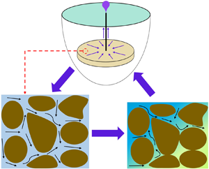
A key implication of (1.6) is the assumption of an invariant permeability coefficient throughout the reservoir. A variety of processes, including inertial losses which are, herein, described by the Forchheimer term in (1.2), are known to cause deviation of the real performance index from the prediction made by (1.6). Also, flow-induced deformation of the solid phase may cause significant changes in the pore structure and permeability of the porous host medium. Figure 1 depicts the inherent coupling between disturbances in the pore fluid pressure and solid phase deformation of a disk-shaped, fluid-producing reservoir through the induced variations in the reservoir rock porosity and permeability. The effect is reported by negative changes in the permeability coefficient in the case of fluid withdrawal from the porous inclusion (Crowdy & Duchemin Reference Crowdy and Duchemin2005; MacMinn, Dufresne & Wettlaufer Reference MacMinn, Dufresne and Wettlaufer2016), and corresponding positive changes in permeability coefficient in the case of fluid injection (Auton & MacMinn Reference Auton and MacMinn2017; Wang et al. Reference Wang, Cheng, Zhang and Ayala2018). The described deformation-induced variation in permeability is a commonly observed mechanism which undermines the validity of linear solutions such as the one shown by (1.6) for fluid transport through deformable porous rocks.

Figure 1. Permeability variation due to coupled fluid flow and solid deformation in a confined porous medium.
Modelling the change in permeability due to the interplay between fluid flow and solid deformation of porous materials has been a vibrant subject of research. Empirical formulae that relate the permeability coefficient to the local pore fluid pressure have been offered for this purpose (Sommer & Mortensen Reference Sommer and Mortensen1996; Zhu, Du & Li Reference Zhu, Du and Li2018). Mechanistic approaches include formulating porosity as a function of both the local pore fluid pressure and the local mean stress or volumetric strain while applying standard correlations between permeability and porosity (Macminn et al. Reference MacMinn, Dufresne and Wettlaufer2016; Sabet et al. Reference Sabet, Barisik, Mobedi and Beskok2019). The permeability–pressure relationships that have been used in the related analytical solutions often follow simple correlations between the permeability and pore fluid pressure (Zoback & Byerlee Reference Zoback and Byerlee1975; Kikani & Pedrosa Reference Kikani and Pedrosa1991) or volumetric strain (Shi & Durucan Reference Shi and Durucan2004). However, the directional dependence of the permeability tensor on changes in the stress or strain tensors allows for and enables preferential orientation of the pore fluid flow in response to pressure gradients (Wong Reference Wong2003; Kang et al. Reference Kang, Lei, Dentz and Juanes2019). A second drawback of the existing permeability models is that the permeability coefficient change is formulated as a function of the local pore pressure change (Zoback & Byerlee Reference Zoback and Byerlee1975; Kikani & Pedrosa Reference Kikani and Pedrosa1991). While permeability is particularly dependent on the local kinematic strain, the strain of an arbitrary point in the porous medium is a non-local function of the pore fluid pressure distribution throughout the entire disturbed volume (Geertsma Reference Geertsma1973; Segall Reference Segall1992).
The motivation for the present study arises from the need for prediction of the observed, yet less-studied, manifestations of the coupling between pore fluid flow and solid deformation of subsurface reservoir rocks in their flow rate-dependent producibility or injectivity (Aulisa et al. Reference Aulisa, Ibragimov, Valko and Walton2009; Dempsey et al. Reference Dempsey, Kelkar, Davatzes, Hickman and Moos2015). These reservoirs are often embedded at a finite depth below the surface of the earth crust (Pegler et al. Reference Pegler, Maskell, Daniels and Bickle2017; Szulczewski, Hesse & Juanes Reference Szulczewski, Hesse and Juanes2013; Segall Reference Segall1992). Therefore, they are quite commonly modelled as porous, fluid-saturated inclusions in a semi-infinite medium representing the subsurface (Rajapakse & Senjuntichai Reference Rajapakse and Senjuntichai1993; Segall Reference Segall1992; Pan Reference Pan2019).
This paper reports a nonlinear and non-local analytical solution for the steady-state Darcy–Forchheimer fluid flow through a disk-shaped porous elastic inclusion embedded within an elastic half-space. The solution accounts for the nonlinear variations in the permeability coefficient due to deformation-induced permeability change while integrating the inherent nonlinearity of the pore fluid pressure gradients due to the considered non-Darcy fluid flow regime, represented by (1.2). The schematics of the fluid flow problem are illustrated in figure 2. Injection or withdrawal of fluid takes place through a cylindrical cavity at the centre of the reservoir, which hereafter is referred to as the inclusion. The semi-infinite elastic medium, which hereafter is referred to as the matrix, is in welded contact with the inclusion.

Figure 2. Schematics of radial fluid flow through the porous inclusion in an elastic half-space.
The considered model of figure 2 entails the following assumptions:
• The disk-shaped inclusion is porous and fluid saturated.
• The fluid flow rate Q at the inner cavity boundary, $r = {r_w}$, is constant.
• The steady state of pore fluid flow throughout the inclusion is reached.
• The initial state of the porous inclusion is isotropic and homogeneous.
• The inclusion, as well as the surrounding half-space matrix, are both linearly elastic.
• The effect of cavity size on the deformation of the inclusion and matrix is negligible.
• Aside from permeability, all properties of the inclusion are invariant.
• The inclusion is in welded contact with the surrounding matrix. That is, the boundary tractions and solid phase displacements at the interface of the inclusion and matrix are identical.
• There is no fluid flow or disturbances of the pore fluid pressure in the semi-infinite matrix outside of the inclusion.

The classical solution for a nucleus of strain (Mindlin & Cheng Reference Mindlin and Cheng1950a,Reference Mindlin and Chengb) is used as a Green's function to formulate the non-local relationship between the pore fluid pressure distribution and elastic strain tensor of the inclusion in the semi-infinite elastic matrix. A linear relationship between the principal components of the strain and permeability coefficient tensors is considered. A perturbation solution technique is developed to simultaneously treat the nonlinearities arising from the deformation-induced variations in the inclusion permeability coefficient and the inertia-dominated component of the pore fluid flow regime. The solution is applied to the problem of fluid injection into or production from the centre of a disk-shaped reservoir embedded within the subsurface. Results are used to offer extended formulations for the commonly used performance index of production or injection wells in deformable porous reservoirs. The significant departure of the obtained performance index from the associated linear model is discussed. New dimensionless groups of parameters are introduced to describe the nonlinear, non-local and coupled nature of the pore fluid flow and solid deformation in the considered poroelastic inclusion problem. By virtue of the insight gained from the definition of these dimensionless groups, the sensitivity of the solution to the key problem parameters, as well as its asymptotic behaviours in the limiting special cases when either or both of the considered nonlinear mechanisms vanish, is discussed and rationalized.
2. The nonlinear permeability coefficient
This section elaborates on the nonlinearities involved in the permeability of the porous inclusion in figure 2. Section 2.1 derives a formula for the apparent permeability coefficient from the Darcy–Forchheimer equation for the pore fluid flow. Section 2.2 derives a separate formula for the variation of the permeability coefficient due to elastic deformation of the inclusion. Lastly, the obtained formulae are assimilated to describe the combined impact of the two mechanisms in terms of a single expression for the effective permeability of the deforming porous inclusion.
2.1. The Darcy–Forchheimer flow through the inclusion
The governing equation for steady-state, radial flow of the pore fluid through the inclusion can be expressed as
 \begin{equation}\frac{1}{r}\frac{\textrm{d}}{{\textrm{d}r}}(rv) = 0. \end{equation}
Equation (2.1) is subjected to the following boundary conditions at the inner and outer boundaries of the inclusion:
 \begin{gather}v = \frac{Q}{{2{{\rm \pi} }rh}}(r = {r_w}),\end{gather}
 \begin{gather}p = 0(r = {r_e}),\end{gather}
where the symbol p refers to the change in pore fluid pressure from the initial pore pressure of the inclusion at the undisturbed state and Q is the pore fluid flow rate across the inner boundary of the inclusion at  $r = {r_w}$. It takes a positive value for fluid withdrawal from the inclusion and a negative value for fluid injection into the inclusion.
The Darcy–Forchheimer equation shown in (1.2) can be rearranged into the scalar form
 \begin{equation}\beta \gamma {v^2} + \frac{\mu }{k}v - \|{\boldsymbol{\nabla}p}\| = 0.\end{equation}
Equation (2.4) can be solved for v to give
 \begin{equation}v = \frac{k}{\mu }\frac{2}{{1 + \sqrt {1 + \frac{{4\beta \gamma {k^2}}}{{{\mu ^2}}}\|{\boldsymbol{\nabla}p}\| } }}\|{\boldsymbol{\nabla}p}\| ,\end{equation}
where  $\|{\boldsymbol{\nabla}p}\| $ is the norm of the pressure gradient vector. The following definition of the apparent permeability ${k_a}$ is made in such a way that (2.5) mimics Darcy's linear law of fluid flow through porous media:
 \begin{equation}\boldsymbol{\bar{v}} = - \frac{{{k_a}}}{\mu }{\boldsymbol{\nabla}}p,\end{equation}
where
 \begin{equation}{k_a} = {k_\epsilon }\frac{2}{{1 + \sqrt {1 + \frac{{4\beta \gamma k_\epsilon ^2}}{{{\mu ^2}}}\|{\boldsymbol{\nabla}p}\|} }};\end{equation} ${k_\epsilon }$ in (2.7) is the intrinsic material permeability after accounting for the solid deformation effect, which will be discussed in the next section. Therefore, the mathematical model shown in (2.1)–(2.3) can be rewritten as
 \begin{gather}\frac{1}{r}\frac{\textrm{d}}{{\textrm{d}r}}\left( {{k_a}r\frac{{\textrm{d}p}}{{\textrm{d}r}}} \right) = 0,\end{gather}
 \begin{gather}{k_a}\frac{{\textrm{d}p}}{{\textrm{d}r}} = \frac{{Q\mu }}{{2{{\rm \pi} }hr}}(r = {r_w}),\end{gather}
 \begin{gather}p = 0(r = {r_e}).\end{gather}
2.2. Deformation-induced permeability variation
A linear relationship between the permeability tensor and the local strain tensor is considered, as follows (Wong Reference Wong2003):
 \begin{equation}\left[ {\begin{array}{@{}c@{}} {{k_1}/{k_{1,0}}}\\ {{k_2}/{k_{1,0}}}\\ {{k_3}/{k_{1,0}}} \end{array}} \right] = \left[ {\begin{array}{@{}c@{}} 1\\ {{k_{2,0}}/{k_{1,0}}}\\ {{k_{3,0}}/{k_{1,0}}} \end{array}} \right] + \left[ {\begin{array}{@{}ccc@{}} a&b&b\\ b&a&b\\ b&b&a \end{array}} \right]\left[ {\begin{array}{@{}c@{}} {{\epsilon_1}}\\ {{\epsilon_2}}\\ {{\epsilon_3}} \end{array}} \right],\end{equation}
where  ${k_1}$, ${k_2}$ and ${k_3}$ are the permeabilities in three principal strain directions, and ${k_{i,0}}$ denotes the initial value of the permeability components; ${\epsilon _1},{\epsilon _2}$ and ${\epsilon _3}$ are the induced principal strains, respectively; and a and b are two dimensionless coefficients which can be determined through the simultaneous tri-axial compression and core flooding experiments (Wong Reference Wong2003; Lin, Chen & Jin Reference Lin, Chen and Jin2017). The absolute value of parameter b is usually larger than a, owing to stronger sensitivity of the permeability along an arbitrary direction to the strain component in the other principal directions (Wong Reference Wong2003; Bai et al. Reference Bai, Meng, Elsworth and Roegiers1999). By assuming an isotropic initial permeability ${k_0}$ to the system, (2.11) can be rewritten as
 \begin{equation}\left[ {\begin{array}{@{}c@{}} {{k_1}/{k_0}}\\ {{k_2}/{k_0}}\\ {{k_3}/{k_0}} \end{array}} \right] = \left[ {\begin{array}{@{}{c}@{}} 1\\ 1\\ 1 \end{array}} \right] + \left[ {\begin{array}{@{}ccc@{}} a&b&b\\ b&a&b\\ b&b&a \end{array}} \right]\left[ {\begin{array}{@{}c@{}} {{\epsilon_1}}\\ {{\epsilon_2}}\\ {{\epsilon_3}} \end{array}} \right].\end{equation}
 The axisymmetric Green's function due to rings of pore fluid pressure change in semi-infinite space is adopted to find the non-local function of the solid phase strain during fluid injection or withdrawal. Detailed formulations of the Green's functions and the associated volume integrals are given in appendix A. The in-plane and anti-plane shear strain components  ${\epsilon _{r\theta }}$ and ${\epsilon _{rz}}$ are assumed to be zero due to the symmetry and relatively small thickness of the considered inclusion geometry compared to its burial depth, i.e. $(1 - {d_1}/{d_2}) \ll 1$, with ${d_1}$ and ${d_2}$ being the top and bottom depths of the porous inclusion. Therefore, the inclusion principal strains are aligned with the axes of the polar coordinate system of figure 2. From (2.12), the following equation for radial permeability is derived for both the fluid withdrawal and injection cases:
 \begin{equation}{k_{rr\epsilon }} = {k_0}(1 + a{\epsilon _{rr}} + b{\epsilon _{\theta \theta }} + b{\epsilon _{zz}}),\end{equation}
where  ${k_{rr\epsilon }}$ is the permeability along radial direction after accounting for the strain change, and ${\epsilon _{rr}}, {\epsilon _{\theta \theta }}$ and ${\epsilon _{zz}}$ are the induced strain components along the radial, circumferential and vertical directions.
Substituting the expressions for  ${\epsilon _{rr}},{\epsilon _{\theta \theta }}$ and ${\epsilon _{zz}}$ from (A10)–(A12) of appendix A into (2.13) yields
 \begin{align}k_{rr\epsilon}[{p_\forall}(r),z] & = {k_0}\left\{ 1 +
\int_{{d_1}}^{{d_2}} \int_0^{{r_e}} \left[
\dfrac{{\partial p(\rho )}}{{\partial \rho }}\left(
a\dfrac{{\partial u_r^{(1)}(r,z;\rho ,\zeta )}}{{\partial
r}} + b\dfrac{{u_r^{(1)}(r,z;\rho ,\zeta )}}{r}\right)\right.\right.\nonumber\\
& \quad \qquad \ \ \, + \left.\left. bp(\rho)\dfrac{{\partial {{\hat{u}}_z}(r,z;\rho ,\zeta
)}}{{\partial z}} \right]\,\textrm{d}\rho\,\textrm{d}\zeta \vphantom{\left(
a\dfrac{{\partial u_r^{(1)}(r,z;\rho ,\zeta )}}{{\partial
r}} + b\dfrac{{u_r^{(1)}(r,z;\rho ,\zeta )}}{r}\right)}\right\},\end{align}
\begin{align}k_{rr\epsilon}[{p_\forall}(r),z] & = {k_0}\left\{ 1 +
\int_{{d_1}}^{{d_2}} \int_0^{{r_e}} \left[
\dfrac{{\partial p(\rho )}}{{\partial \rho }}\left(
a\dfrac{{\partial u_r^{(1)}(r,z;\rho ,\zeta )}}{{\partial
r}} + b\dfrac{{u_r^{(1)}(r,z;\rho ,\zeta )}}{r}\right)\right.\right.\nonumber\\
& \quad \qquad \ \ \, + \left.\left. bp(\rho)\dfrac{{\partial {{\hat{u}}_z}(r,z;\rho ,\zeta
)}}{{\partial z}} \right]\,\textrm{d}\rho\,\textrm{d}\zeta \vphantom{\left(
a\dfrac{{\partial u_r^{(1)}(r,z;\rho ,\zeta )}}{{\partial
r}} + b\dfrac{{u_r^{(1)}(r,z;\rho ,\zeta )}}{r}\right)}\right\},\end{align}
where r and z in (2.14) are the radius and depth of the observation point;  $\rho $ and $\zeta $ are the radius and depth of the pressure source; and p is the magnitude of the pressure source.
The parameters  $u_r^{(1)}$ and ${\hat{u}_z}$ in (2.14) are Green's functions for the radial and vertical displacements. While detailed derivations of these functions are presented in appendix A, the end results are presented here, as follows:
 \begin{gather}u_r^{(1)} = - \frac{{\rho {c_m}}}{2}[{I^{ - \theta (z - \zeta )}}(1,1;0) + (3 - 4v){I^{(z + \zeta )}}(1,1;0) - 2z{I^{(z + \zeta )}}(1,1;1)],\end{gather}
 \begin{gather}{\hat{u}_z} = - \frac{{\rho {c_m}}}{2}[\theta {I^{ - \theta (z - \zeta )}}(0,0;1) + (3 - 4v){I^{(z + \zeta )}}(0,0;1) + 2z{I^{(z + \zeta )}}(0,0;2)],\end{gather}
where the poroelastic uniaxial compaction coefficient  ${c_m} = \alpha (1 - 2v)/2G(1 - v)$ is defined in (A5); $\alpha $ and v are the Biot–Willis effective stress coefficient and Poisson's ratio; $\theta = - 1$ for $z \ge \zeta $ and $\theta = 1$ for $z \lt \zeta $; and G is the shear modulus of the material. The term ${I^c}(n,m;t)$ in (2.15) and (2.16) denotes the Lipschitz–Hankel family of integrals, which is defined as follows (Eason, Noble & Sneddon Reference Eason, Noble and Sneddon1955):
 \begin{equation}{I^c}(n,m;t) = \int_0^\infty {{s^t}} {J_n}(s\rho ){J_m}(sr)\,{\textrm{e}^{ - cs}}\,\textrm{d}s,\end{equation}
where  $J_n$ is the $n\textrm{th}$-order Bessel function of the first kind. For certain values of $n,m$ and t, the Lipschitz–Hankel integral ${I^c}(n,m;t)$ can be written in terms of closed-form formulae. The expressions for these integrals are given in appendix B.
For a disk-shaped inclusion with small thickness, i.e.  $(1 - {d_1}/{d_2}) \ll 1$, the variation of pore fluid pressure and permeability along the vertical direction can be neglected. This assumption reduces (2.14) to the following equation:
 \begin{align}
{k_{rr\epsilon }}(r) &= {k_{rr\epsilon }}[{p_\forall }(r),{d_m}]\nonumber\\
&= {k_0}\left\{ 1 + \int_{{d_1}}^{{d_2}}
\int_0^{{r_e}} \left[ \dfrac{\partial p(\rho )}{\partial \rho}
\left( {a\dfrac{{\partial u_r^{(1)}}}{{\partial r}}(r,{d_m};\rho ,\zeta ) + b\dfrac{{u_r^{(1)}(r,{d_m};\rho ,\zeta )}}{r}} \right)\right. \right.\nonumber\\
& \quad \qquad \ \ \, + \left.\left. bp(\rho )\dfrac{{\partial {{\hat{u}}_z}}}{{\partial z}}(r,{d_m};\rho ,\zeta ) \right]\,\textrm{d}\rho \,\textrm{d}\zeta \vphantom{\left\{ 1 + \int_{{d_1}}^{{d_2}}
\int_0^{{r_e}} \left[ \dfrac{\partial p(\rho )}{\partial \rho}
\left( {a\dfrac{{\partial u_r^{(1)}}}{{\partial r}}(r,{d_m};\rho ,\zeta ) + b\dfrac{{u_r^{(1)}(r,{d_m};\rho ,\zeta )}}{r}} \right)\right. \right.}\right\},
\end{align}
\begin{align}
{k_{rr\epsilon }}(r) &= {k_{rr\epsilon }}[{p_\forall }(r),{d_m}]\nonumber\\
&= {k_0}\left\{ 1 + \int_{{d_1}}^{{d_2}}
\int_0^{{r_e}} \left[ \dfrac{\partial p(\rho )}{\partial \rho}
\left( {a\dfrac{{\partial u_r^{(1)}}}{{\partial r}}(r,{d_m};\rho ,\zeta ) + b\dfrac{{u_r^{(1)}(r,{d_m};\rho ,\zeta )}}{r}} \right)\right. \right.\nonumber\\
& \quad \qquad \ \ \, + \left.\left. bp(\rho )\dfrac{{\partial {{\hat{u}}_z}}}{{\partial z}}(r,{d_m};\rho ,\zeta ) \right]\,\textrm{d}\rho \,\textrm{d}\zeta \vphantom{\left\{ 1 + \int_{{d_1}}^{{d_2}}
\int_0^{{r_e}} \left[ \dfrac{\partial p(\rho )}{\partial \rho}
\left( {a\dfrac{{\partial u_r^{(1)}}}{{\partial r}}(r,{d_m};\rho ,\zeta ) + b\dfrac{{u_r^{(1)}(r,{d_m};\rho ,\zeta )}}{r}} \right)\right. \right.}\right\},
\end{align}
where  ${d_m} = ({d_1} + {d_2})/2$ is the middle depth of the porous inclusion.
Subsequently, the permeability variation due to solid deformation will be coupled with the Darcy–Forchheimer flow model. According to (2.7), the apparent permeability along the radial direction for radial fluid flow into or away from the centre of a disk, considering both the solid phase deformation and the Forchheimer flow, can be written as
 \begin{gather}{k_{rra}} = {k_{rr\epsilon }}\frac{2}{{1 + \sqrt {1 + \frac{{4\beta \gamma k_{rr\epsilon }^2}}{{{\mu ^2}}}\left|{\frac{{\textrm{d}p}}{{\textrm{d}r}}} \right|} }},\end{gather}
 \begin{gather}\beta = \frac{{0.005}}{{k_{rr\epsilon }^{0.5}{\phi ^{5.5}}}},\end{gather}
where  ${k_{rr\epsilon }}$ is the radial intrinsic permeability that accounts for the pore deformation.
3. Solution to the fluid flow problem
By substituting (2.19) into (2.8)–(2.10) the radial flow through the inclusion can be formulated, as follows:
 \begin{gather}\frac{1}{r}\frac{\textrm{d}}{{\textrm{d}r}}\left\{ {{k_{rra}}[{p_\forall }(r)]r\frac{{\textrm{d}p}}{{\textrm{d}r}}} \right\} = 0,\end{gather}
 \begin{gather}{k_{rra}}[{p_\forall }(r)]r\frac{{\textrm{d}p}}{{\textrm{d}r}} = \frac{{Q\mu }}{{2{{\rm \pi} }h}}(r = {r_w}),\end{gather}
 \begin{gather}p = 0(r = {r_e}),\end{gather}
where the apparent permeability coefficient  ${k_{rra}}[{p_\forall }(r)]$ is given by (2.19) and incorporates both the solid deformation and the inertial forces of the fluid flow. The subscript $\forall $ in this context reiterates the non-local dependence of the permeability coefficient. That is, ${k_{rra}}$ is determined by the pore fluid pressure distribution throughout the entire volume of the inclusion.
By taking the first integral of (3.1) and applying the inner boundary condition of (3.2), the considered mathematical problem is reduced to a first-order nonlinear differential equation, as follows:
 \begin{gather}{k_{rra}}[{p_\forall }(r)]r\frac{{\textrm{d}p}}{{\textrm{d}r}} = \frac{{Q\mu }}{{2{{\rm \pi} }h}},\end{gather}
 \begin{gather}p({r_e}) = 0.\end{gather}
 Equation (3.4) is nonlinear due to the non-local and variant nature of the permeability coefficient  ${k_{rra}}[{p_\forall }(r)]$. A perturbation technique is implemented to mathematically treat the involved nonlinearities. For this purpose, the left side of (3.4) is decomposed into a linear part pertaining to the initial permeability of the inclusion, ${k_0}$, and a nonlinear part, as follows:
 \begin{equation}\frac{{\textrm{d}p}}{{\textrm{d}r}} + \frac{{\delta k({p_\forall })}}{{{k_0}}}\frac{{\textrm{d}p}}{{\textrm{d}r}} = \frac{{Q\mu }}{{2{{\rm \pi} }hr{k_0}}},\end{equation}
where  $\delta k(p)$ in (3.6) is expressed as
 \begin{equation}\delta k({p_\forall }) = {k_{rr\epsilon }}\frac{2}{{1 + \sqrt {1 + \frac{{4\beta \gamma k_{rr\epsilon }^2}}{{{\mu ^2}}}\left|{\frac{{\textrm{d}p}}{{\textrm{d}r}}} \right|} }} - {k_0}.\end{equation}
 A perturbation series expansion of the pore fluid pressure in terms of the small parameter  $\varepsilon = 1/G$ is sought, as follows:
 \begin{equation}p(r;\varepsilon ) = {p_0}(r) + \varepsilon {p_1}(r) + {\varepsilon ^2}{p_2}(r) + \cdots + {\varepsilon ^n}{p_n}(r) + O({\varepsilon ^{n + 1}}),\end{equation}
where G is the shear modulus of the solid phase skeleton of the porous inclusion. The zeroth-order perturbation solution  ${p_0}(r)$ pertains to the familiar steady-state, radial Darcy flow of the pore fluid through the inclusion when the permeability is assumed to be constant and equal to the initial permeability of the system. The expression for ${p_0}(r)$ can be conveniently obtained as
 \begin{equation}{p_0}(r) = \frac{{Q\mu }}{{2{{\rm \pi} }h{k_0}}}\ln \left( {\frac{r}{{{r_e}}}} \right).\end{equation}
Substitution of (3.8) into (3.6) decomposes the original nonlinear differential equation into a sequence of linear equations, as shown in (3.10) through (3.13).
The zeroth-order differential equation is
 \begin{equation}\frac{{\textrm{d}{p_0}}}{{\textrm{d}r}} = \frac{{Q\mu }}{{2{{\rm \pi} }hr{k_0}}}.\end{equation}
The first-order differential equation is
 \begin{equation}\frac{{\textrm{d}{p_1}}}{{\textrm{d}r}} + \psi ({p_\forall })\frac{{\textrm{d}{p_0}}}{{\textrm{d}r}} = 0.\end{equation}
The second-order differential equation is
 \begin{equation}\frac{{\textrm{d}{p_2}}}{{\textrm{d}r}} + \psi ({p_\forall })\frac{{\textrm{d}{p_1}}}{{\textrm{d}r}} = 0.\end{equation}
The nth-order differential equation is
 \begin{equation}\frac{{\textrm{d}{p_n}}}{{\textrm{d}r}} + \psi ({p_\forall })\frac{{\textrm{d}{p_{n - 1}}}}{{\textrm{d}r}} = 0.\end{equation}
The parameter  $\psi ({p_\forall })$ in (3.10)–(3.13) is given by
 \begin{equation}\psi ({p_\forall }) = G\left( {\dfrac{{{k_{rr\epsilon }}}}{{{k_0}}}\dfrac{2}{{1 + \sqrt {1 + \dfrac{{4\beta \gamma k_\epsilon^2}}{{{\mu^2}}}\left|{\dfrac{{\textrm{d}p}}{{\textrm{d}r}}} \right|} }} - 1} \right).\end{equation}
Detailed mathematical derivations of the described decomposition are presented in appendix C. Likewise, the following set of boundary conditions is obtained:
 \begin{equation}{p_0}({r_e}) = {p_1}({r_e}) = {p_2}({r_e}) = {p_n}({r_e}) = 0.\end{equation}
 Equations (3.10) through (3.13) are a set of linear first-order differential equations. The analytical solution to these equations up to the desired order of accuracy can be obtained through a sequential procedure. Detailed steps of deriving the perturbation solution are demonstrated in appendix D. The result for the  $n\textrm{th}$-order solution $p_n^\ast (r)$ can be expressed through a recursive equation of the following compact form:
 \begin{equation}p_n^\ast (r) = \frac{{Q\mu }}{{2{{\rm \pi} }h{k_0}}}\left\{ {\ln \left( {\frac{r}{{{r_e}}}} \right) + \mathop \sum \limits_{i = 1}^n \frac{{{{( - 1)}^{i + 1}}}}{{k_0^i}}\int_r^{{r_e}} {\dfrac{{\prod\limits_{j = 0}^{i - 1} {\delta k[p_{j\forall }^\ast (r)]} }}{r}} \,\textrm{d}r} \right\},\end{equation}
in which
 \begin{equation}\delta k[{p_\forall }(r)] = {k_{rr\epsilon }}[{p_\forall }(r)]\dfrac{2}{{1 + \sqrt {1 + \dfrac{{4\beta \gamma k_{rr\epsilon }^2}}{{{\mu ^2}}}\left|{\dfrac{{\textrm{d}p}}{{\textrm{d}r}}} \right|} }} - {k_0}.\end{equation}
 Once the general solution for the pore fluid pressure redistribution due to the considered steady-state flow is found, the  $n\textrm{th}$-order perturbation solution for the well performance index is obtained from the following equation:
 \begin{equation}J_n^\ast = - \frac{Q}{{p_n^\ast ({r_w})}}.\end{equation}
4. Solution verification against finite element simulation results
The presented analytical solution is herein validated against the numerical, finite element solution to the same problem. For this purpose, fluid production from a disk-shaped inclusion within an elastic half-space is simulated in COMSOL® Multiphysics (COMSOL® Multiphysics 2018). The semi-infinite matrix is represented by an axisymmetric numerical model. The dimensions of the numerical model of the semi-infinite matrix in the lateral and vertical directions are 100 and 30 times larger than the inclusion radius and depth, respectively. The matrix and inclusion are discretized using an adaptive mesh of unstructured, triangular finite elements with quadratic shape functions. Figure 3 shows the dimensions of the finite element solution domain, while figure 4 gives a partial view of the numerical grid. Built-in linear elastic finite elements are used for the numerical domain representing the matrix outside of the inclusion (COMSOL® Multiphysics 2018). Built-in poroelastic finite elements are used to discretize the inclusion domain (COMSOL® Multiphysics 2018). These elements account for the coupling between the pore fluid flow and solid phase deformation of the porous inclusion. The apparent permeability model of the Darcy–Forchheimer flow in COMSOL® Multiphysics is the same as the one shown in (2.19). This model is used to describe the constitutive relation of the pore fluid flow through the inclusion in the numerical model.

Figure 3. The dimensions of the finite element model.

Figure 4. Numerical mesh for the finite element analysis in COMSOL® Multiphysics.
The well performance index parameter for the case of fluid withdrawal  $(Q \gt 0)$ is calculated using both COMSOL® Multiphysics and the proposed analytical model. The basic parameters of the test case are summarized in table 1. The first-order and second-order perturbation solutions are compared with the numerical results in figure 5. The following three cases are considered. The first case considers only the influence of Forchheimer flow while the effect of solid deformation is neglected ( $\beta \ne 0$ and $a,b = 0$). The second case considers only the effect of solid deformation on material permeability without accounting for the nonlinear term of Forchheimer flow ( $\beta = 0$ and $a,b \ne 0$). The third case considers both the Forchheimer flow and solid deformation effects ( $\beta \ne 0$ and $a,b \ne 0$).
Table 1. The parameters of the base case study.


Figure 5. Comparison of the performance index calculated from the analytical and numerical solutions.
Owing to strong nonlinearity of the problem, the accuracy of the first-order perturbation solution, particularly for higher production rates, is inadequate. However, in all of the considered cases, the second-order perturbation solution closely follows the numerical solution with a relative error not exceeding 1.0 %. Therefore, the second-order perturbation solution is considered accurate and used in the following discussion of the results.
5. Discussion of results
5.1. Linear Darcy flow with nonlinear solid deformation effect
In this section, only the effect of solid deformation is considered in the analysis. That is,  $\beta = 0$ in (2.19) while $a,b \ne 0$ in (2.18). The parameters shown in table 1 are used for this purpose. The rate of contrast (%) in values of the well performance index between the nonlinear, perturbation solution and the linear, flow-only solution is demonstrated through the parameter $\Delta J$, which is defined as follows:
 \begin{equation}\Delta J = \frac{{{J_{nl}} - {J_l}}}{{{J_l}}} \times 100\,\%.\end{equation}
Here,  ${J_{nl}}$ is obtained from (3.18) and accounts for the induced permeability variation; ${J_l}$ is the performance index obtained from the linear, flow-only solution that assumes a constant permeability. The analytical expression for ${J_l}$ is shown in (1.6).
Variations of  $\Delta J$ versus well flow rate are presented in figure 6. Each panel in figure 6 is divided into two regions: the upper region pertains to fluid injection whereas the lower region demonstrates the decline of $\Delta J$ resulting from fluid withdrawal.

Figure 6. The sensitivity of the nonlinear performance index to the problem parameters: (a) shear modulus; (b) initial permeability; (c) Biot–Willis effective stress coefficient; (d) Poisson's ratio; (e) the inclusion depth; (f) permeability–strain correlation coefficients.
The conventional linear solution in figure 6 returns a constant performance index against the changes in flow rate. However, a continuous increase or decline of performance index is observed via the nonlinear solution when increasing the injection or withdrawal flow rates. For the fluid production case, the rate of increase in the magnitude of  $\Delta J$ accelerates with increasing well flow rate. Conversely, a reverse trend, i.e. decelerating deviation of the nonlinear solution from the linear solution, is observed in the fluid injection case. Consequently, the observed value of $\Delta J$ in the fluid withdrawal case is larger than that of the injection case. The reason is that a higher withdrawal rate will cause a larger reduction of permeability, as well as a larger decrease in the pore fluid pressure. In such a case, the two effects enhance each other. Conversely, the induced permeability enhancement and pore pressure build-up for the fluid injection case would induce opposite effects in such a way that they negate each other. Therefore, the slope of the $\Delta J\textrm{ versus }Q$ curve decreases with the increase of well injection rate.
The effect of varying constitutive parameters of the porous reservoir on the performance index is shown in each panel. Figure 6(a) indicates a more substantial change in  $\Delta J$ for smaller shear modulus. Figure 6(b) shows the effect of initial permeability on the well performance index. The nonlinear effect is more pronounced for smaller permeability coefficients. Figure 6(c) reveals that the change in well performance index is more sensitive to flow rate in the case of larger Biot–Willis coefficients. The reason is that a higher Biot coefficient results in a higher effect of pore fluid pressure changes on the rock stress or strain. A larger Poisson's ratio with the same shear modulus causes a larger bulk modulus and, therefore, a stiffer solid skeleton of the rock. For this reason, figure 6(d) shows that the well performance index for a rock with smaller Poisson's ratio is more influenced by the increase in flow rate. From figure 6(e) it can be inferred that the well performance index shows negligible sensitivity to depth change at large depth, while a notable enhancement in $\Delta J$ is seen at extremely shallow depths. Figure 6(f) shows the impact of the stress-sensitive coefficients a and b on well performance; larger values of a and b indicate a stronger dependence of material permeability on rock strain components, and thus a more significant deviation of well performance index from the linear solution.
Practical implications of the observed trends in enhanced or impaired permeability upon cyclic injection and production of the subsurface fluid are enumerated, as follows. An isolated standpoint of the coupling between pore fluid pressure and rock solid deformation advocates that, for an alternating sequence of fluid injection and production operations, each cycle should be first started by fluid injection, so that an increased well performance index is attained prior to the subsequent production phase. Figure 7 shows that each complete injection–production cycle will conclude by a higher average well performance index than the scenario in which the alternating cycles start with fluid production.

Figure 7. The schematics showing variations of the well performance index for a fluid injection–production cycle.
5.2. Darcy–Forchheimer flow without solid deformation effect
This section considers the nonlinear Forchheimer flow through the porous inclusion without accounting for the effect of solid phase deformation on the permeability coefficient. That is,  $\beta \ne 0$ in (2.19) while $a,b = 0$ in (2.18). The parameters shown in table 1 are used in the analysis. Equation (1.2) demonstrates that the Forchheimer flow is mainly affected by four parameters, namely, the intrinsic permeability, porosity, fluid viscosity and fluid density. The effects of these parameters on the well performance index for both fluid injection and production processes are presented in figure 8. In addition, the Reynolds number for the fluid flow near the wellbore is plotted against the well flow rate in figure 8.

Figure 8. The effect of the parameters of Forchheimer flow on the well performance index. (a) Initial permeability; (b) porosity; (c) fluid viscosity; (d) fluid density. The solid curves denote  $\Delta J$ during fluid production; the hollow circles denote $\Delta J$ during fluid injection; the dashed curves denote Reynolds number of fluid flow near the inclusion inner boundary during fluid injection or production.
Unlike the conclusions drawn for the solid deformation effects, the inertial-loss component of fluid flow in the porous inclusion will reduce the well performance index upon fluid injection or withdrawal. Further, the magnitudes of  $\Delta J$ for both cases are identical. The reason is that the Forchheimer term in (1.2) is not affected by the direction of the flow velocity. Higher boundary flow rates Q will amplify the Forchheimer flow effect because the inertial losses would be more significant at the corresponding higher Reynolds numbers.
Figure 8(a) further shows that an increase in intrinsic permeability would make the effect of the Forchheimer flow more substantial, since a higher permeability will enhance the fluid velocity, thus resulting in a more dominant effect of the inertial forces. The opposite trend is the case in figure 8(b), where the Forchheimer flow effect is stronger for smaller inclusion porosity. The reason can be inferred from the dependence of the Forchheimer parameter  $\beta $ on porosity from (1.5). Likewise and for similar reasons, figures 8(c) and 8(d) reveal that the Forchheimer flow becomes more pronounced with the decrease of fluid viscosity and the increase of fluid density.
5.3. Darcy–Forchheimer flow with solid deformation effect
The combined effect of the two considered mechanisms is herein considered. That is,  $\beta \ne 0$ in (2.19) and $a,b \ne 0$ in (2.18). Figure 9 shows variations of the well performance index using the parameter values shown in table 1 and for different values of the initial permeability and shear modulus. Variation trends of $\Delta J$ are similar to those in figures 6(a) and 6(b). However, the magnitudes of $\Delta J$ variation among the two sets of plots are different. Compared to figure 6, figure 9 demonstrates a larger $\Delta J$ in the case of fluid withdrawal from the inclusion and a smaller $\Delta J$ for fluid injection. The reason is that the inertial effects impose further resistance to fluid transport against a given pressure gradient regardless of the flow direction. Therefore, the Forchheimer flow hampers the favourable effect of pore space dilation during fluid injection. Conversely, the combined effect of Forchheimer flow and solid deformation would result in more significant reduction in the performance index during fluid production from the inclusion.

Figure 9. Variations of  $\Delta J$ versus flow rate for different values of the initial permeability and shear modulus: (a) initial permeability; (b) shear modulus.
The comparable effect of either mechanism on the overall performance index of the inclusion is demonstrated in figure 10. For this purpose, a new set of parameters is presented in table 2. These parameters are used to investigate the changes in the performance index at a fixed flow rate of  $|Q |= 500\,{\textrm{m}^3}\,\textrm{da}{\textrm{y}^{ - 1}}$ against variations of the inclusion initial permeability and shear modulus.

Figure 10. Variations of  $\Delta J$ versus initial permeability and shear modulus at a fixed well flow rate of 500 m3 day−1: (a) initial permeability; (b) shear modulus.
Table 2. Parameters of the case study with comparable effects of solid deformation and Forchheimer flow.

Figure 10(a) demonstrates different trends in variations of  $\Delta J$ upon fluid injection and production; the combined effect of solid deformation and Forchheimer flow will always reduce the performance index when withdrawing fluid from the inclusion since both mechanisms tend to enhance the resistance against fluid flow. However, the solid deformation mechanism dominates the Forchheimer flow effect when the initial permeability is small. Therefore, the absolute value of the deviation from the linear solution, $\Delta J$, decreases when increasing the initial permeability. The trend reverses when the initial permeability is higher because the effect of Forchheimer flow on $\Delta J$ is stronger for the resulting higher flow velocities.
In the fluid injection case, figures 10(a) and 10(b) indicate a change in the sign of  $\Delta J$ from positive to negative when the inclusion initial permeability increases. Dilation of the pore space in such a case dominates the effect of the Forchheimer flow, resulting in a positive $\Delta J$ when the initial permeability is relatively small. However, the Forchheimer flow transcends the solid deformation effect at larger initial permeabilities, thus causing an injectivity index that is smaller than the injectivity index of the linear solution. It is also found that, for higher values of the initial permeability and shear modulus, the $\Delta J$ curves for production and injection will both asymptotically approach the $\Delta J$ of the solution that only considers the Forchheimer flow mechanism. This is because the effect of solid deformation diminishes for larger values of permeability or shear modulus. An analysis of such asymptotic behaviour is further enumerated in § 5.4.
5.4. Dimensionless groups and spatial distributions of pore fluid pressure
The distributions of the pore fluid pressure change and the permeability change during fluid production are plotted against radial distance from the inclusion centre point in figure 11. The effects of both considered mechanisms, i.e. solid mechanics and Forchheimer flow, are incorporated in the case study using the parameters listed in table 1. The solid curves in figure 11 show the relative magnitude of the nonlinear portion of the pore fluid pressure, through the parameter  $\chi = ({p_{nl}} - {p_l})/{p_l}$ in which ${p_{nl}}$ and ${p_l}$ denote the nonlinear and linear pressure solutions. The dashed curves represent the ratio of apparent permeability reduction to initial permeability $(\psi = \delta k/{k_0})$. Figure 11 shows a substantial reduction in apparent radial permeability throughout the inclusion. The effect, however, is more drastic in the general vicinity of the inclusion inner boundary, owing to the larger pore fluid pressure decline within the same region.

Figure 11. The profiles of the normalized, nonlinear proportion of pore fluid pressure, as well as the normalized nonlinear change in the inclusion permeability.
The zeroth-order solution described by (3.9) can be rearranged in the following form:
 \begin{equation}{p_{0D}} = \ln ({r_D}).\end{equation}
Equation (5.2) adequately describes the radial Darcy flow of fluid through the inclusion by the following general definitions of the dimensionless pressure  ${p_D}$ and radius ${r_D}$:
 \begin{gather}{p_D} = \frac{{2{{\rm \pi} }h{k_0}p(r)}}{{Q\mu }},\end{gather}
 \begin{gather}{r_D} = \frac{r}{{{r_e}}}.\end{gather}
Discussion of (1.3) and (1.4) demonstrated that the Darcy–Forchheimer flow regime involves the dimensionless Reynolds number  $Re$. Likewise, the deformation-induced component of the nonlinear flow is controlled by a dimensionless parameter ${C_{mD}}$ that would scale the poroelastic uniaxial compaction coefficient of the inclusion porous skeleton, appearing in (2.15) and (2.16), with the flow-induced pressure gradients. Since this parameter has the dimensions of inverse pressure, a natural choice for the scaling factor would be a coefficient similar to the case of ${p_D}$ in (5.3). The following dimensionless group is thus suggested:
 \begin{equation}{C_{mD}} = \frac{{|Q|\mu {c_m}}}{{2{{\rm \pi} }h{k_0}}}.\end{equation}
A high Reynolds number implies that the effect of inertial losses on the fluid flow is more significant. This conclusion was previously demonstrated in figure 8, where the relative magnitude of reduction in the performance index parameter compared to the linear solution,  $\Delta J$, was shown to increase with $Re$. Likewise, a large value of ${C_{mD}}$ would enhance the deformation-induced effects. The matter is demonstrated through the series of sensitivity analyses in figure 6, where smaller parameters G, $\nu $ and ${k_0}$, or a larger value of $\alpha $, are shown to enhance the nonlinear deviation of the performance index parameter from the linear solution.
Consequently, the ratio  $\Lambda = R{e_{rw}}/{C_{mD}}$ constitutes a new dimensionless group that quantifies the relative magnitude of the inertial losses effect compared to the solid deformation effect on the deviation of pore fluid pressure from the linear solution represented by (5.2). The value of $\Lambda$ can be derived from (1.4) and (5.5), as follows:
 \begin{equation}\Lambda = \frac{{k_0^2\beta \gamma }}{{{c_m}{\mu ^2}{r_w}}}.\end{equation}
When  $\Lambda \to 0$, the general solution obtained in (3.16) is expected to render the special-case solution of § 5.1 which incorporates only the solid deformation-induced effects $(\beta = 0)$. Conversely, the asymptotic behaviour of (3.16) when $\Lambda \to \infty $ is expected to reduce the general solution of (3.16) to the special-case solution which only includes the Forchheimer term of (1.3), i.e. when $a = b = 0$. Figure 12 confirms this insight.

Figure 12. The distribution of normalized pressure deviation from the linear solution at the fixed flow rate of 500 m3 day−1: (a)  $\Lambda = 935\,349$; (b) $\Lambda = 35\,076$; (c) $\Lambda = 5916$; (d) $\Lambda = 555$.
Figure 12(a–d) show the profiles of the nonlinear pressure deviation  $\chi $ along the radial distance $\, r/{r_e}$ for a series of four successively descending $\Lambda $ values. Figure 12(a) indicates that at the highest $\Lambda $ value, the pressure distribution considering both mechanisms mimics the pressure distribution obtained from the solution which considers only the Forchheimer flow effect. Conversely, when the value of $\Lambda $ is small, figure 12(d) demonstrates that the pressure solution incorporating both mechanisms closely follows the pressure solution that considers only the solid deformation effect. Figures 12(b) and 12(c) demonstrate the transition of the general pore pressure solution incorporating the combined nonlinear effects from the Forchheimer-only asymptote to the solid deformation-only asymptote, for intermediate values of $\Lambda $.
6. Conclusions
An analytical perturbation solution for the nonlinear problem of Darcy–Forchheimer flow in a disk-shaped, porous, elastic inclusion embedded in a semi-infinite, elastic medium is presented. The solution captures the assimilated nonlinearities arising from the non-local dependence of deformation-induced permeability throughout the inclusion volume, as well as the local inertial losses of flow through the pore space of the inclusion. Results are used to offer a flow rate-dependent extension of the linear, rate-independent formulations for the performance index parameter that is commonly used to assess the ability of porous rocks in delivering the pore fluids toward or away from a wellbore during the subsurface production or injection of fluids.
Findings indicate that most significant changes in the apparent permeability coefficient occur in close vicinity of the inclusion inner boundary. However, these variations are large enough to cause a significant impact on the performance index. Further, the deformation-induced nonlinearities in the considered problem do not affect the production and injection cases symmetrically; deviation of the performance index from the prediction of a constant-permeability, linear solution is larger in the case of fluid production than in the injection case. Parametric analysis of the solution results shows that increases in shear modulus, initial permeability and Poisson's ratio of the inclusion will reduce the nonlinear changes in the performance index. Conversely, an increase of the Biot–Willis coefficient will enhance the effect. Darcy–Forchheimer flow without solid deformation will induce equal impacts on the well performance index for fluid production and injection. The combined effect of solid deformation and Forchheimer flow would always result in decline of the performance index in the case of fluid production. However, the two mechanisms would negate each other when fluid is injected into the inclusion, causing a positive or negative deviation from the linear solution for the performance index depending on the dominant mechanism.
The combined effect of the considered nonlinear mechanisms, i.e. elastic deformation of the inclusion and inertial losses of the pore fluid flow, is represented by two dimensionless groups that govern the magnitude of the deviation of the nonlinear solution from the linear solution. The asymptotic behaviours of flow through porous inclusion for extremely small or large values of the ratio of these dimensionless groups are shown to render the special cases when the effect of either nonlinear mechanism in the solution is forced to vanish.
Acknowledgement
Support from a Wilson Research Initiation Grant of the College of Earth and Mineral Sciences at Pennsylvania State University is gratefully acknowledged. The authors wish to thank the anonymous referees for their constructive criticism of this work.
Declaration of interests
The authors report no conflict of interest.
Appendix A. Nucleus-of-strain solution in half-space
Nucleus of strain refers to the elastic singularity of an infinitesimally small cubic volume subjected to three orthogonal double forces of the same magnitude. Figure 13 shows the schematics of such a singularity. It can be shown that a point source of pore fluid pressure change is mathematically equivalent to a nucleus of strain (Geertsma Reference Geertsma1973; Wang Reference Wang2000). The analytical solution for the stress and displacements induced by a nucleus of strain in a semi-infinite domain is derived in Mindlin & Cheng (Reference Mindlin and Cheng1950a,Reference Mindlin and Chengb).

Figure 13. The schematics of a ring-shaped nucleus of strain in a semi-infinite domain.
The non-local strain and stress fields of the resulting elastic field imply that the point source of pore fluid pressure change alters the solid stress/strain of an arbitrary point within a porous elastic medium. Thus, the nucleus-of-strain solution can be used as the Green's function and integrated over the entire volume of inclusion.
The axisymmetric symmetry of the considered disk-shaped inclusion in figure 13 justifies the use of the axisymmetric Green's function for the nucleus of strain given in Segall (Reference Segall1992). The displacement field  $u(r,z)$ due to the distribution of pore fluid pressure disturbances can be formulated as
 \begin{equation}{u_i}(r,z) = \int_{{d_1}}^{{d_2}} {\int_0^\infty {p(\rho ,\zeta )\, {{\hat{u}}_i}(r,z;\rho ,\zeta )\,\textrm{d}\rho \,\textrm{d}\zeta } ,} \end{equation}
where u is the displacement at the observation point and  ${\hat{u}_i}$ is the Green's function for the induced displacement along the i direction caused by a ring-shaped pressure source. Green's functions of the displacement components are obtained by Segall (Reference Segall1992), as follows:
 \begin{gather}{\hat{u}_r} = \frac{{\rho {c_m}}}{2}[{\textrm{I}^{ - \theta (z - \zeta )}}(0,1;1) + (3 - 4v){\textrm{I}^{(z + \zeta )}}(0,1;1) - 2z{\textrm{I}^{(z + \zeta )}}(0,1;2)],\end{gather}
 \begin{gather}{\hat{u}_z} = - \frac{{\rho {c_m}}}{2}[\theta {I^{ - \theta (z - \zeta )}}(0,0;1) + (3 - 4v){I^{(z + \zeta )}}(0,0;1) + 2z{I^{(z + \zeta )}}(0,0;2)],\end{gather}
where  $\theta = - 1$ for $z \ge \zeta $ and $\theta = 1$ for $z \lt \zeta $. The notation ${I^c}(n,m;t)$ is defined as
 \begin{equation}{I^c}(n,m;t) = \int_0^\infty {{s^t}{J_n}(s\rho ){J_m}(sr)\,{\textrm{e}^{ - cs}}\,\textrm{d}s} .\end{equation}
The parameter  ${c_m}$ is known as the uniaxial compaction coefficient in the poromechanics literature. It can be derived as follows:
 \begin{equation}{c_m} = \frac{{\alpha (1 - 2v)}}{{2G(1 - v)}}.\end{equation}
 For certain values of n, m and t, the infinite integral in (A4) can be expressed using closed-form expressions so that significant computational cost can be saved. However, it is difficult to express  ${I^c}(0,1;1)$ and ${I^c}(0,1;2)$ in (A2) in terms of such functions. Therefore, (A1) is integrated by parts by defining $u_r^{(1)} = \smallint {\hat{u}_r}\,\textrm{d}\rho$ and honouring $\smallint \rho {J_0}(s\rho )\,\textrm{d}\rho = {s^{ - 1}}\rho {J_1}(s\rho )$ (Segall Reference Segall1992). As a result, the radial and vertical displacements can be calculated by
 \begin{gather}{u_r}(r,z) = \int_{{d_1}}^{{d_2}} {\int_0^\infty {\frac{{\partial p(\rho ,\zeta )}}{{\partial \rho }}\, u_r^{(1)}(r,z;\rho ,\zeta )\,\textrm{d}\rho \,\textrm{d}\zeta ,} } \end{gather}
 \begin{gather}{u_z}(r,z) = \int_{{d_1}}^{{d_2}} {\int_0^\infty {p(\rho ,\zeta )\, {{\hat{u}}_z}(r,z;\rho ,\zeta )\,\textrm{d}\rho \,\textrm{d}\zeta } } ,\end{gather}
 \begin{gather}u_r^{(1)} = - \frac{{\rho {c_m}}}{2}[{I^{ - \theta (z - \zeta )}}(1,1;0) + (3 - 4v){I^{(z + \zeta )}}(1,1;0) - 2z{I^{(z + \zeta )}}(1,1;1)],\end{gather}
 \begin{gather}{\hat{u}_z} = - \frac{{\rho {c_m}}}{2}[\theta {I^{ - \theta (z - \zeta )}}(0,0;1) + (3 - 4v){I^{(z + \zeta )}}(0,0;1) + 2z{I^{(z + \zeta )}}(0,0;2)].\end{gather}
Appendix B shows the analytical expressions of all the Lipschitz–Hankel integrals involved in (A8) and (A9). After expressing  $u_r^{(1)}$ and ${\hat{u}_z}$ in terms of closed-form equations by substituting (B1)–(B5) into (A8) and (A9), the strain solutions can be readily calculated as
 \begin{gather}{\epsilon _{rr}} = \frac{{\partial {u_r}}}{{\partial r}} = \int_{{d_1}}^{{d_2}} {\int_0^\infty {\frac{{\partial p(\rho ,\zeta )}}{{\partial \rho }}\frac{{\partial u_r^{(1)}(r,z;\rho ,\zeta )}}{{\partial r}}\,\textrm{d}\rho \,\textrm{d}\zeta ,} }\end{gather}
 \begin{gather}{\epsilon _{\theta \theta }} = \frac{{{u_r}}}{r} = \int_{{d_1}}^{{d_2}} {\int_0^\infty {\frac{{\partial p(\rho ,\zeta )}}{{\partial \rho }}\frac{{u_r^{(1)}(r,z;\rho ,\zeta )}}{r}\,\textrm{d}\rho \,\textrm{d}\zeta } } ,\end{gather}
 \begin{gather}{\epsilon _{zz}} = \frac{{\partial {u_z}}}{{\partial z}} = \int_{{d_1}}^{{d_2}} {\int_0^\infty {p(\rho ,\zeta )\frac{{\partial {{\hat{u}}_z}(r,z;\rho ,\zeta )}}{{\partial z}}\,\textrm{d}\rho \,\textrm{d}\zeta .} } \end{gather}
Appendix B. Lipschitz–Hankel integrals
Calculation of the displacement solutions involves four integrals of the type shown in (A4), namely,  ${I^c}(1,1;0),{I^c}(1,1;1),{I^c}(0,0;1)$ and ${I^c}(0,0;2)$. These integrals can be expressed using closed-form equations, as follows (Van Deun & Cools Reference Van Deun and Cools2008; Eason et al. Reference Eason, Noble and Sneddon1955):
 \begin{gather}{I^c}(1,1;0) = \frac{1}{{{{\rm \pi} }\sqrt {r\rho } }}{Q_{1/2}}\left( {\frac{{{r^2} + {\rho^2} + {c^2}}}{{2r\rho }}} \right),\end{gather}
 \begin{gather}{I^c}(0,0;1) = \frac{{c{\kappa ^3}E(\kappa )}}{{4{{\rm \pi} }(1 - {\kappa ^2}){{(\rho r)}^{3/2}}}},\end{gather}
where
 \begin{equation}\kappa = \sqrt {4r\rho /[{{(\rho + r)}^2} + {c^2}]} .\end{equation}
Here,  ${Q_n}$ in (B1) is the Legendre function of the second kind and degree n and $E(\kappa )$ is the complete elliptic integral of the second kind. The values of ${I^c}(1,1;1)$ and ${I^c}(0,0;2)$ are obtained via the following recursive differential formula (Eason et al. Reference Eason, Noble and Sneddon1955):
 \begin{gather}{I^c}(1,\, 1;1) = - \frac{\partial }{{\partial c}}{I^c}(1,1;0),\end{gather}
 \begin{gather}{I^c}(0,\, 0;2) = - \frac{\partial }{{\partial c}}{I^c}(0,0;1).\end{gather}
Appendix C. Perturbation solution to the nonlinear flow equation
The steady-state fluid flow is governed by the following diffusion equation and boundary conditions:
 \begin{gather}\frac{1}{r}\frac{\textrm{d}}{{\textrm{d}r}}\left\{ {{k_{rra}}[{p_\forall }(r)]r\frac{{\textrm{d}p}}{{\textrm{d}r}}} \right\} = 0,\end{gather}
 \begin{gather}{k_{rra}}[{p_\forall }(r)]r\frac{{\textrm{d}p}}{{\textrm{d}r}} = \frac{{Q\mu }}{{2{{\rm \pi} }h}}(r = {r_w}),\end{gather}
 \begin{gather}p = 0(r = {r_e}).\end{gather}
Integration of (C1) yields
 \begin{equation}{k_{rra}}[{p_\forall }(r)]r\frac{{\textrm{d}p}}{{\textrm{d}r}} = {C_1}.\end{equation}
From (C2) an expression for  ${C_1}$ is obtained as
 \begin{equation}{C_1} = \frac{{Q\mu }}{{2{{\rm \pi} }h}}.\end{equation}
Therefore, (C1) is reduced to the first-order differential equation
 \begin{gather}{k_{rra}}[{p_\forall }(r)]r\frac{{\textrm{d}p(r)}}{{\textrm{d}r}} = \frac{{Q\mu }}{{2{{\rm \pi} }h}},\end{gather}
 \begin{gather}p({r_e}) = 0.\end{gather}
Equation (C6) can be decomposed into a linear part and a nonlinear part, as follows:
 \begin{equation}{k_{rra}}({p_\forall }) = {k_0} + \delta k({p_\forall }),\end{equation}
where  ${k_0}$ denotes the initial permeability. The expression of $\delta k({p_\forall })$ is derived as
 \begin{equation}\delta k({p_\forall }) = {k_{rr\epsilon }}\frac{2}{{1 + \sqrt {1 + \dfrac{{4\beta \gamma k_\epsilon ^2}}{{{\mu ^2}}}\left|{\dfrac{{\textrm{d}p}}{{\textrm{d}r}}} \right|} }} - {k_0}.\end{equation}
Therefore, (C6) can be rearranged to give
 \begin{equation}\frac{{\textrm{d}p}}{{\textrm{d}r}} + \frac{{\delta k({p_\forall })}}{{{k_0}}}\frac{{\textrm{d}p}}{{\textrm{d}r}} = \frac{{Q\mu }}{{2{{\rm \pi} }hr{k_0}}}.\end{equation}
 A small parameter  $\varepsilon = 1/G$ is selected to apply the perturbation technique. Consequently, (C10) is converted to the following form:
 \begin{equation}\frac{{\textrm{d}p}}{{\textrm{d}r}} + \varepsilon \psi ({p_\forall })\frac{{\textrm{d}p}}{{\textrm{d}r}} = \frac{{Q\mu }}{{2{{\rm \pi} }hr{k_0}}},\end{equation}
where  $\psi (p)$ is defined as
 \begin{equation}\psi ({p_\forall }) = \frac{{\delta k({p_\forall })}}{{\varepsilon {k_0}}} = \frac{{G\delta k({p_\forall })}}{{{k_0}}} = G\left( {\frac{{{k_{rr\epsilon }}}}{{{k_0}}}\frac{2}{{1 + \sqrt {1 + \dfrac{{4\beta \gamma k_\epsilon^2}}{{{\mu^2}}}\left|{\dfrac{{\textrm{d}p}}{{\textrm{d}r}}} \right|} }} - 1} \right).\end{equation}
A perturbation series expansion of the pore fluid pressure is sought, as follows:
 \begin{equation}p(r;\varepsilon ) = {p_0}(r) + \varepsilon {p_1}(r) + {\varepsilon ^2}{p_2}(r) + \cdots + {\varepsilon ^n}{p_n}(r) + O({\varepsilon ^{n + 1}}).\end{equation}
Substitution in (C11) yields
 \begin{gather}\dfrac{{\textrm{d}{p_0}}}{{\textrm{d}r}} + \varepsilon \left[ {\dfrac{{\textrm{d}{p_1}}}{{\textrm{d}r}} + \psi ({p_\forall })\dfrac{{\textrm{d}{p_0}}}{{\textrm{d}r}}} \right] + {\varepsilon ^2}\left[ {\dfrac{{\textrm{d}{p_2}}}{{\textrm{d}r}} + \psi ({p_\forall })\dfrac{{\textrm{d}{p_1}}}{{\textrm{d}r}}} \right] + \cdots + {\varepsilon ^n}\left[ {\dfrac{{\textrm{d}{p_n}}}{{\textrm{d}r}} + \psi ({p_\forall })\dfrac{{\textrm{d}{p_{n - 1}}}}{{\textrm{d}r}}} \right]\nonumber\\ +\, {\varepsilon ^{n + 1}}\psi ({p_\forall })\dfrac{{\textrm{d}{p_n}}}{{\textrm{d}r}} + O({\varepsilon ^{n + 1}}) = \dfrac{{Q\mu }}{{2{{\rm \pi} }hr{k_0}}}.\end{gather}
By collecting like powers of  $\varepsilon $ while neglecting the higher-order terms, the following series of $(n + 1)$ linear differential equations is obtained.
The zeroth-order differential equation is
 \begin{equation}\frac{{\textrm{d}{p_0}}}{{\textrm{d}r}} = \frac{{Q\mu }}{{2{{\rm \pi} }hr{k_0}}}.\end{equation}
The first-order differential equation is
 \begin{equation}\frac{{\textrm{d}{p_1}}}{{\textrm{d}r}} + \psi ({p_\forall })\frac{{\textrm{d}{p_0}}}{{\textrm{d}r}} = 0.\end{equation}
The second-order differential equation is
 \begin{equation}\frac{{\textrm{d}{p_2}}}{{\textrm{d}r}} + \psi ({p_\forall })\frac{{\textrm{d}{p_1}}}{{\textrm{d}r}} = 0.\end{equation}
The nth-order differential equation is
 \begin{equation}\frac{{\textrm{d}{p_n}}}{{\textrm{d}r}} + \psi ({p_\forall })\frac{{\textrm{d}{p_{n - 1}}}}{{\textrm{d}r}} = 0,\end{equation}
with the following outer boundary conditions:
 \begin{equation}{p_0}({r_e}) = {p_1}({r_e}) = {p_2}({r_e}) = {p_n}({r_e}) = 0.\end{equation}
Appendix D. Analytical solution to the linear differential equations
The solution to the zeroth-order linear equation that is shown in (C15) recovers the conventional, linear, steady-state flow and associated distribution of pore fluid pressure, as follows:
 \begin{equation}{p_0} = \frac{{Q\mu }}{{2{{\rm \pi} }h{k_0}}}\ln \left( {\frac{r}{{{r_e}}}} \right).\end{equation}
 The solution for  ${p_1}$ can be obtained by substituting the ${p_0}$ solution into the first-order differential equation shown in (C16),
 \begin{equation}\frac{{\textrm{d}{p_1}}}{{\textrm{d}r}} + \psi ({p_{0\forall }})\frac{{Q\mu }}{{2{{\rm \pi} }hr{k_0}}} = 0.\end{equation}
Equation (D2) can be integrated to give
 \begin{equation}\int_{{p_1}}^{{P_1}({r_e})} {\textrm{d}{p_1}} = - \frac{{Q\mu }}{{2{{\rm \pi} }h{k_0}}}\int_r^{{r_e}} {\frac{{\psi ({p_{0\forall }})}}{r}\,\textrm{d}r} = - \frac{{Q\mu }}{{2{{\rm \pi} }h\varepsilon k_0^2}}\int_r^{{r_e}} {\frac{{\delta k({p_{0\forall}})}}{r}\,\textrm{d}r} .\end{equation}
Applying the boundary condition from (C19) yields
 \begin{equation}{p_1} = \frac{{Q\mu }}{{2{{\rm \pi} }h\varepsilon k_0^2}}\int_r^{{r_e}} {\frac{{\delta k({p_{0\forall }})}}{r}\,\textrm{d}r} .\end{equation}
Hence, the first-order pore pressure solution can be obtained as
 \begin{equation}p_1^\ast (r) = {p_0}(r) + \varepsilon {p_1}(r) = \frac{{Q\mu }}{{2{{\rm \pi} }h{k_0}}}\ln \left( {\frac{r}{{{r_e}}}} \right) + \frac{{Q\mu }}{{2{{\rm \pi} }hk_0^2}}\int_r^{{r_e}} {\frac{{\delta k[{p_{0\forall }}(r)]}}{r}\,\textrm{d}r} .\end{equation}
 For the second-order linear equation, the term  $\textrm{d}{p_1}/\textrm{d}r$ can be obtained by taking the derivative of ${p_1}$. The term $\psi ({p_\forall })$ can be obtained by substituting $p_1^\ast $ into $\delta k({p_\forall })$ in (C9). Therefore, integration of the differential equation (C17) yields
 \begin{equation}\int_{{p_2}}^{{P_2}({r_e})} {\textrm{d}{p_2}} = \frac{{Q\mu }}{{2{{\rm \pi} }h{k_0}}}\int_r^{{r_e}} {\frac{{\psi [{p_{0\forall }}(r)]\psi [p_{1\forall }^\ast (r)]}}{r}\,\textrm{d}r} .\end{equation}
By using (C19), the solution of the second-order equation is obtained as
 \begin{equation}{p_2} = - \frac{{Q\mu }}{{2{{\rm \pi} }hk_0^3{\varepsilon ^2}}}\int_r^{{r_e}} {\frac{{\delta k[{p_{0\forall }}(r)]\delta k[p_{1\forall }^\ast (r)]}}{r}\,\textrm{d}r} .\end{equation}
Hence, the second-order perturbation solution can be expressed as
 \begin{align} p_2^\ast = {p_0} + \varepsilon {p_1} + {\varepsilon ^2}{p_2} &= \dfrac{{Q\mu }}{{2{{\rm \pi} }h{k_0}}}\ln \left( {\dfrac{r}{{{r_e}}}} \right) + \dfrac{{Q\mu }}{{2{{\rm \pi} }hk_0^2}}\int_r^{{r_e}} {\dfrac{{\delta k[{p_{0\forall }}(r)]}}{r}\,\textrm{d}r} \nonumber\\ &\quad - \dfrac{{Q\mu }}{{2{{\rm \pi} }hk_0^3}}\int_r^{{r_e}} {\dfrac{{\delta k[{p_{0\forall }}(r)]\delta k[p_{1\forall }^\ast (r)]}}{r}\,\textrm{d}r} . \end{align}
Similarly, the solution to the nth-order linear equation (C18) is obtained as follows:
 \begin{equation}{p_n} = {( - 1)^{n + 1}}\frac{{Q\mu }}{{2{{\rm \pi} }hk_0^{n + 1}{\varepsilon ^n}}}\int_r^{{r_e}} {\frac{{\delta k[p_{({n - 1} )\forall }^\ast (r)]\delta k[p_{(n - 2)\forall }^\ast (r)] \ldots \delta k[{p_{0\forall }}(r)]}}{r}\,\textrm{d}r} .\end{equation}
Thus, the nth-order perturbation solution for the pore fluid pressure can be expressed as
 \begin{align} p_n^\ast (r) &= \dfrac{{Q\mu }}{{2{{\rm \pi} }h{k_0}}}\ln \left( {\dfrac{r}{{{r_e}}}} \right) + \dfrac{{Q\mu }}{{2{{\rm \pi} }hk_0^2}}\int_r^{{r_e}} {\dfrac{{\delta k[{p_{0\forall }}(r)]}}{r}\,\textrm{d}r} - \dfrac{{Q\mu }}{{2{{\rm \pi} }hk_0^3}}\int_r^{{r_e}} {\dfrac{{\delta k[p_{1\forall }^\ast (r)]\delta k[{p_{0\forall }}(r)]}}{r}\,\textrm{d}r}\nonumber \\ & \quad + \cdots + {( - 1)^{n + 1}}\dfrac{{Q\mu }}{{2{{\rm \pi} }hk_0^{n + 1}}}\int_r^{{r_e}} {\dfrac{{\prod\limits_{i = 0}^{n - 1} {\delta k[p_{i\forall }^\ast (r)]} }}{r}\,\textrm{d}r,} \end{align}
where
 \begin{gather}\delta k(p) = {k_{rr\epsilon }}(p)\frac{2}{{1 + \sqrt {1 + \frac{{4\beta \gamma k_{rr\epsilon }^2}}{{{\mu ^2}}}\left|{\frac{{\textrm{d}p}}{{\textrm{d}r}}} \right|} }} - {k_0},\end{gather}
 \begin{gather}{k_{rr\epsilon }}(p) = {k_0}\left\{ {1 + \int_{{d_1}}^{{d_2}} {\int_0^{{r_e}} {\left[ {\frac{{\partial p(\rho )}}{{\partial \rho }}\left( {a\frac{{\partial u_r^{(1)}}}{{\partial r}} + b\frac{{u_r^{(1)}}}{r}} \right) + bp(\rho )\frac{{\partial {{\hat{u}}_z}}}{{\partial z}}} \right]} } \,\textrm{d}\rho \,\textrm{d}\zeta } \right\}.\end{gather}


 Open access