


1. Introduction
Secondary currents (SCs) are ubiquitous features of straight open-channel flows (OCFs). They appear as helical motions in time-averaged velocity fields near the channel sidewalls where they are generated due to turbulence anisotropy (Einstein & Li Reference Einstein and Li1958; Nezu & Nakagawa Reference Nezu and Nakagawa1993). Such SCs may also be generated throughout the channel cross-section if the bed roughness and/or topography are heterogeneous in the transverse direction. Such transverse heterogeneity can occur naturally in rivers, for example due to sand ridges (Colombini Reference Colombini1993) or due to a preferential alignment of aquatic plant patches. The SCs influence bed friction and mixing of nutrients within aquatic ecosystems (e.g. Nikora & Roy Reference Nikora and Roy2012) and therefore need to be accounted for in river modelling and stream management.
There has been growing interest in bed-surface-induced SCs with studies focusing on different flow types (e.g. boundary layer, closed channel, pipe and OCFs) and different surface heterogeneities, such as streamwise topographical ridges (e.g. Wang & Cheng Reference Wang and Cheng2006; Vanderwel & Ganapathisubramani Reference Vanderwel and Ganapathisubramani2015; Hwang & Lee Reference Hwang and Lee2018; Medjnoun, Vanderwel & Ganapathisubramani Reference Medjnoun, Vanderwel and Ganapathisubramani2018; Yang & Anderson Reference Yang and Anderson2018; Medjnoun, Vanderwel & Ganapathisubramani Reference Medjnoun, Vanderwel and Ganapathisubramani2020; Zampiron, Cameron & Nikora Reference Zampiron, Cameron and Nikora2020a; Zampiron et al. Reference Zampiron, Nikora, Cameron, Patella, Valentini and Stewart2020b), flat alternating strips with different surface roughness (e.g. Willingham et al. Reference Willingham, Anderson, Christensen and Barros2014; Anderson et al. Reference Anderson, Barros, Christensen and Awasthi2015; Stroh et al. Reference Stroh, Hasegawa, Kriegseis and Frohnapfel2016; Bai, Kevin & Monty Reference Bai, Kevin and Monty2018; Stroh et al. Reference Stroh, Schäfer, Frohnapfel and Forooghi2020; Wangsawijaya et al. Reference Wangsawijaya, Baidya, Chung, Marusic and Hutchins2020) and converging/diverging surface patterns (e.g. Nugroho, Hutchins & Monty Reference Nugroho, Hutchins and Monty2013; Kevin et al. Reference Kevin, Bai, Pathikonda, Nugroho, Barros, Christensen and Hutchins2017; Kevin & Hutchins Reference Kevin and Hutchins2019; Anderson Reference Anderson2020). Despite these recent efforts, there remains a shortage of systematic data to elucidate the nature of SCs for different flow types and bed-surface heterogeneities. The key findings of the studies cited above include (among others): (i) the size of the SC cells generally scales with the transverse spacing of ridges/strips until it reaches values comparable in size to the outer flow scale (e.g. flow depth or boundary layer thickness) and (ii) the rotation direction of the SC cells appears to place upflow regions near smooth topographical ridges and downflow regions near high-roughness flat strips (e.g. Nezu & Nakagawa Reference Nezu and Nakagawa1993). However, highly rough ridges (composed of streamwise-aligned rows of line-filling pyramidal obstacles) where both pressure and viscous drag contribute to bed friction have been shown by Yang & Anderson (Reference Yang and Anderson2018) to exhibit an opposite rotation direction of SC cells compared to previously studied smooth ridges. Considering smooth triangular-shaped ridges on a hydraulically rough bed, it has been noted that (iii) the contribution of SCs to the overall friction factor depends on their size, attaining a maximum when they are comparable to the flow depth (Zampiron et al. Reference Zampiron, Cameron and Nikora2020a,b). A similar conclusion follows from the study of Nikora et al. (Reference Nikora, Stoesser, Cameron, Stewart, Papadopoulos, Ouro, McSherry, Zampiron, Marusic and Falconer2019), who investigated bed friction mechanisms in rough-bed OCFs. The mechanism regulating the friction at the bed appeared to be related to the interplay between turbulence and SCs. Specifically, Zampiron et al. (Reference Zampiron, Cameron and Nikora2020a) explored the interaction between turbulence and SCs and found using premultiplied velocity spectra that the appearance of SCs suppressed the turbulent very-large-scale motions (VLSMs) that would otherwise be present. Attenuation of spectral energy at large wavelengths, although not as pronounced, has also been observed for other types of spanwise wall heterogeneities (e.g. Awasthi & Anderson Reference Awasthi and Anderson2018; Barros & Christensen Reference Barros and Christensen2019). Furthermore, (iv) the instantaneous manifestations of the SCs have been found to meander laterally in time (e.g. Kevin & Hutchins Reference Kevin and Hutchins2019; Wangsawijaya et al. Reference Wangsawijaya, Baidya, Chung, Marusic and Hutchins2020; Zampiron et al. Reference Zampiron, Cameron and Nikora2020a). Zampiron et al. (Reference Zampiron, Cameron and Nikora2020a) found a linear relationship between the streamwise wavelength associated with the meandering (named ‘secondary current instability’) and the vorticity thickness, suggesting that the meandering is due to inflection instabilities induced by the spanwise gradient of streamwise velocity introduced by the SCs themselves.
The objective of this study is to further explore SC–turbulence interactions by considering momentum and energy exchanges for uniform OCFs with ridge-induced SCs, using double-averaged (in space and time) conservation equations. The double-averaging methodology (e.g. Nikora et al. Reference Nikora, McEwan, McLean, Coleman, Pokrajac and Walters2007) provides a useful framework to study roughness- and/or topography-induced SCs as it neatly partitions momentum and energy fluxes into turbulence and SC contributions. For a steady, two-dimensional and uniform double-averaged flow, the momentum and energy balances are reduced to a form with the dependence of their terms only on the wall-normal distance, simplifying assessment of the scaling properties of turbulence and SC statistics. This flow type is the focus of this paper. To provide an underpinning background, the relevant double-averaged momentum and energy conservation equations are outlined in § 2. In § 3, the experimental methodology and flow conditions are detailed, while in §§ 4 and 5 the results and key conclusions of this work are presented, respectively.
2. Double-averaged conservation equations
2.1. Double-averaged momentum balance
The double-averaged momentum conservation equation for flows over fixed beds can be presented as (e.g. Nikora et al. Reference Nikora, McEwan, McLean, Coleman, Pokrajac and Walters2007)
 \begin{align} &\left.\begin{aligned} \phi \frac{\partial \langle \bar{u}_i \rangle}{\partial t} & =\\ \end{aligned}\right\rbrace\text{Time rate of change}\nonumber\\ &\left.\begin{aligned} \phantom{\phi \frac{\partial \langle \bar{u}_i \rangle}{\partial t}} & + \phi g_i -\frac{1}{\rho} \frac{\partial \phi \langle \bar{p} \rangle}{\partial x_i}\\ \end{aligned}\right\rbrace\text{Source}\nonumber\\ &\left.\begin{aligned} \phantom{\phi \frac{\partial \langle \bar{u}_i \rangle}{\partial t}} & - \underbrace{\frac{\partial \phi \langle \bar{u}_i \rangle \langle \bar{u}_j \rangle}{\partial x_j}}_{\text{Mean flow}} - \underbrace{\frac{\partial \phi \langle \tilde{\bar{u}}_i\tilde{\bar{u}}_j \rangle}{\partial x_j}}_{\text{Dispersive}} - \underbrace{\frac{\partial \phi \langle \overline{u'_i u'_j} \rangle}{\partial x_j}}_{\text{Turbulent}} + \underbrace{\frac{\partial}{\partial x_j} \left(\phi \nu \left\langle \overline{ \frac{\partial {u}_i }{\partial x_j}} \right\rangle\right)}_{\text{Viscous}}\\ \end{aligned}\right\rbrace\begin{aligned}\text{Transport}\end{aligned}\nonumber\\ &\left.\begin{aligned} \phantom{\phi \frac{\partial \langle \bar{u}_i \rangle}{\partial t}} & + \frac{\phi}{\rho}\left({\frac{1}{ V_f}\iint\limits_{S_{int}}\bar{p}m_i\,\text{d}S} - {\frac{1}{V_f}\iint\limits_{S_{int}}\rho\nu \frac{\partial \bar{u}_i}{\partial x_j}m_j\,\text{d}S}\right) \end{aligned}\right\rbrace\text{Sink,} \end{align}
where the Einstein summation convention for repeated indices is used;  $t$ is time;
  $x_i$ is the coordinate vector with the
  $i=1,2,3$ components aligned with the streamwise (
 $x$), spanwise (
 $y$) and vertical (
 $z$) coordinates, respectively, and with
  $x_3=z=0$ defined at the level of the roughness troughs
  $z_t=0$ (figure 1b);
  $g_i$ is the gravity acceleration vector;
  $m_i$ is the unit vector normal to the bed surface and directed into the fluid;
  $\rho$ is fluid density;
  $\nu$ is fluid kinematic viscosity; overbars denote time averaging; and angle brackets indicate spatial averaging within thin spatial domains parallel to the mean bed. Note that in (2.1), the pressure gradient is defined as a momentum supply term, although it may generally also serve as a momentum transport term. The intrinsic spatial average of a generic flow variable
  $\theta$ (e.g. pressure or velocity) is defined as
 \begin{equation} \langle\theta\rangle =\frac{1}{V_f}\int_{V_f}{\theta \,\text{d}V}, \end{equation}
where  $V_f(x,y,z)$ is the fluid volume within the averaging domain of volume
  $V_0(z)$. The averaging domain may be defined as a cuboid with side lengths
  $W_x$,
  $W_y$ and
  $W_z$ (figure 1a) chosen to suit the flow field and bed geometry. In OCFs, strong gradients of flow properties in the vertical direction require
  $W_z$ to be as small as possible. The ratio
  $\phi (x,y,z)=V_f$/
 $V_0$ is the roughness geometry function (Nikora et al. Reference Nikora, McEwan, McLean, Coleman, Pokrajac and Walters2007) which is in the range
  $0<\phi <1$ below the roughness tops and
  $\equiv {1}$ above them (figure 1b). The symbol
  $S_{int}$ defines the area of the fluid–bed interface within the averaging domain and thus
 \begin{equation} \iint\limits_{S_{int}}\theta\,\text{d}S \end{equation}
is the integral of  $\theta$ over the interfacial surface (e.g. pressure and viscous drag terms in (2.1)). The velocity vector
  $u_i(x,y,z,t)$, with
  $u_1=u$,
  $u_2=v$ and
  $u_3=w$, is decomposed as
  $u_i = \bar {u}_i+u'_i$, where
  $\bar {u}_i$ is the time-averaged velocity and
  $u'_i$ is a temporal fluctuation. The time-averaged velocity is further decomposed as
  $\bar {u}_i = \langle \bar {u}_i \rangle +\tilde {\bar {u}}_i$, where
  $\langle \bar {u}_i \rangle$ is the double-averaged velocity and
  $\tilde {\bar {u}}_i$ is a spatial fluctuation of time-averaged velocity associated with mean flow heterogeneity due to bed roughness and/or SCs. Similarly, the fluid pressure can be decomposed as
  $p = \bar {p}+p'$ and
  $\bar {p} = \langle \bar {p}\rangle +\tilde {\bar {p}}$. The space- and time-averaging operations are equivalent to convolution of the flow field with an appropriate filter kernel (e.g. Lien, Yee & Wilson Reference Lien, Yee and Wilson2005; Nikora et al. Reference Nikora, McEwan, McLean, Coleman, Pokrajac and Walters2007; Kono, Ashie & Tamura Reference Kono, Ashie and Tamura2010). Therefore, in the general case, double-averaged velocities and pressures retain their dependence on all three spatial coordinates and time, i.e.
  $\langle \bar {u}_i \rangle = f(x,y,z,t)$ and
  $\langle \bar {p} \rangle = f(x,y,z,t)$. Compared to the conventional Reynolds-averaged momentum equation, (2.1) explicitly accounts for the roughness (or bed) geometry and for the effects of dispersive stresses
  $-\rho \langle \tilde {\bar {u}}_i\tilde {\bar {u}}_j \rangle$, viscous drag (i.e.
  $({\iint _{S_{int}}\rho \nu (\partial \bar {u}_i/\partial x_j)m_j\,\text {d}S})/V_f$) and pressure drag (i.e.
  $-({\iint _{S_{int}}\bar {p}m_i\,\text {d}S})/V_f$) at the bed. The viscous and pressure drag terms emerge as a result of spatial averaging; in conventional Reynolds-averaged equations the drag effects are accounted for in the boundary conditions and are not present in the equations themselves.

Figure 1. Averaging domain of volume  $V_0(z)$, roughness geometry function
  $\phi$, maximum and mean flow depths
  $H$ and
  $\hat {H}$ and other key elements of spatial averaging.
Integrating the streamwise ( $i = 1$) momentum balance equation (2.1) from a generic level
  $z$ to the water surface elevation
  $z_{ws}$, introducing
  $g_1 = g \sin \alpha \approx gS_b$, where
  $g$ is gravity acceleration,
  $S_b = \tan (\alpha )$ is bed slope and
  $\alpha$ the angle of the channel bed from horizontal, and simplifying for steady
  $\partial {\langle \bar {\phantom {\varTheta }}\rangle }/\partial {t} = 0$, uniform
  $\partial \langle \bar {\phantom {\varTheta }}\rangle /\partial {x} = 0$ and two-dimensional
  $\langle \bar {v}\rangle = \langle \bar {w}\rangle = \partial \langle \bar {\phantom {\varTheta }}\rangle /\partial {y} = 0$ flow, the following equation is obtained:
 \begin{equation} \rho g S_b \int_z^{z_{ws}} \phi \,\text{d}z ={-}\phi\rho\langle \tilde{\bar{u}}\tilde{\bar{w}}\rangle-\phi\rho \langle \overline{u'w'}\rangle+\phi\rho\nu \left\langle \overline{\frac{\partial {u} }{\partial z}} \right\rangle + \int^{z_{ws}}_z{F_D\,\text{d}z}, \end{equation}
where
 \begin{equation} -\rho\langle \tilde{\bar{u}}\tilde{\bar{w}}\rangle-\rho \langle \overline{u'w'}\rangle+\rho\nu \left\langle \overline{\frac{\partial {u}}{\partial z}} \right\rangle = \tau(z) \end{equation}
is the total fluid stress and
 \begin{equation} F_D(z)=\phi\left(-\frac{1}{V_f}{\iint\limits_{S_{int}}\bar{p}m_1\,\text{d}S} +{\frac{1}{V_f}{ \iint\limits_{S_{int}}\rho\nu \frac{\partial \bar{u}_1}{\partial x_j}m_j\,\text{d}S}}\right) \end{equation}
is the sum of pressure and viscous drag per unit volume. Equation (2.4) describes the flux of gravity-induced momentum in the form of dispersive  $-\rho \langle \tilde {\bar {u}} \tilde {\bar {w}} \rangle$, Reynolds
  $-\rho \langle \overline {u'w'}\rangle$ and viscous
  $\rho \nu \langle \overline {\partial {u}/\partial {z} } \rangle$ stresses, and the sink of momentum at the bed due to drag forces
  $\int _{z}^{z_{ws}}{F_D\,\text {d}z}$. Setting
  $z$ equal to the roughness trough elevation
  $z_t$ in (2.4), the bed shear stress
  $\tau _0$ is obtained as
  $\tau _0 = \rho g S_b \hat {H} = \int ^{z_{ws}}_{z_t}{F_D\,\text {d}z}$, where
  $\hat {H} = \int _{z_t}^{z_{ws}}{\phi \,\text {d}z}$ is the mean flow depth within the
  $x$–
$x$– $y$ extent of the averaging domain. The conventional shear velocity can then be expressed as
  $u_* = \sqrt {\tau _0/\rho } = \sqrt {g\hat {H}S_b}$.
2.2. Double-averaged kinetic energy balance
The double-averaged kinetic energy for flows over fixed beds can be decomposed as
 \begin{equation} \underbrace{\frac{1}{2} \langle \overline{u_i u_i} \rangle}_{\substack{\text{Total}\\\text{kinetic energy}}}=\underbrace{\frac{1}{2} \langle \bar{u}_i \rangle\langle \bar{u}_i \rangle}_{\text{DMKE}}+\underbrace{\frac{1}{2} \langle \tilde{\bar{u}}_i \tilde{\bar{u}}_i \rangle}_{\text{DKE}}+\underbrace{\frac{1}{2} \langle \overline{u'_iu'_i} \rangle}_{\text{SATKE}}, \end{equation}
where the terms on the right-hand side are referred to as the double-mean (DMKE), dispersive (DKE) and spatially averaged turbulent (SATKE) components of the kinetic energy, respectively. Following Papadopoulos et al. (Reference Papadopoulos, Nikora, Cameron, Stewart and Gibbins2020), the conservation equation for DMKE is
 \begin{align} &\left.\begin{aligned} \frac{1}{2}\frac{\partial \phi \langle \bar{u}_i \rangle \langle \bar{u}_i \rangle}{\partial t} & =\\ \end{aligned}\notag\right\rbrace\text{Time rate of change}\nonumber\\ &\quad\left.\begin{aligned} \phantom{XXXXXXX} & +\underbrace{\phi \langle \bar{u}_i \rangle g_i}_{\text{$G$}}\\ \end{aligned}\right\rbrace\text{Source}\nonumber\\ &\quad\left.\begin{aligned} \phantom{XXXXXXX} & +\underbrace{\phi \langle \tilde{\bar{u}}_i \tilde{\bar{u}}_j \rangle \frac{\partial \langle \bar{u}_i\rangle}{\partial x_j}}_{\text{$I_1$}}+\underbrace{\phi \langle \overline{u'_iu'_j} \rangle \frac{\partial \langle \bar{u}_i\rangle}{\partial x_j}}_{\text{$I_2$}}+ \underbrace{\frac{\phi}{\rho}\langle \bar{p} \rangle\frac{\partial \langle \bar{u}_i \rangle}{\partial x_i}}_{\text{ $I_3$}}\\ \phantom{XXXXXXX} & +\underbrace{\frac{\langle \bar{u}_i \rangle}{\rho V_0}\iint\limits_{S_{int}}\bar{p}m_i\, \text{d}S}_{\text{$I_4$}}-\underbrace{ \frac{\langle \bar{u}_i \rangle}{V_0} \iint\limits_{S_{int}}\nu \frac{\partial \bar{u}_i}{\partial x_j}m_j\,\text{d}S}_{\text{$I_5$}} \end{aligned}\right\rbrace\begin{aligned}\text{Interbudget}\\ \text{exchange}\end{aligned}\nonumber\\ &\quad\left.\begin{aligned} \phantom{XXXXXXX} & -\underbrace{\frac{1}{2} \frac{\partial \phi \langle \bar{u}_i \rangle \langle \bar{u}_i \rangle \langle \bar{u}_j \rangle }{\partial x_j}}_{\text{$T_1$}}-\underbrace{\frac{\partial \phi\langle \bar{u}_i \rangle \langle \tilde{\bar{u}}_i \tilde{\bar{u}}_j \rangle}{\partial x_j}}_{\text{$T_2$}}-\underbrace{\frac{\partial \phi \langle \bar{u}_i \rangle \langle \overline{u'_iu'_j} \rangle}{\partial x_j}}_{\text{$T_3$}}\\ \phantom{XXXXXXX} & -\underbrace{\frac{1}{\rho}\frac{\partial \phi \langle \bar{p} \rangle \langle \bar{u}_i \rangle}{\partial x_i}}_{\text{$T_4$}}+ \underbrace{\nu\frac{\partial}{\partial x_j}\left(\langle \bar{u}_i \rangle \frac{\partial \phi\langle \bar{u}_i \rangle}{\partial x_j} \right)}_{\text{$T_5$}}\\ \end{aligned}\right\rbrace\text{Transport}\nonumber\\ &\quad\left.\begin{aligned} \phantom{XXXXXXX} & -\underbrace{\phi\nu \frac{\partial \langle \bar{u}_i \rangle}{\partial x_j} \frac{\partial \langle \bar{u}_i \rangle}{\partial x_j}}_{\text{$D_1$}}-\underbrace{\phi\nu \frac{\partial \langle \bar{u}_i \rangle}{\partial x_j}\left\langle \frac{\partial \tilde{\bar{u}}_i }{\partial x_j}\right\rangle}_{\text{$D_2$}}\\ \end{aligned}\right\rbrace\text{Dissipation to heat,} \end{align}
the conservation equation for DKE is
 \begin{align} &\left.\begin{aligned} \frac{1}{2}\frac{\partial \phi \langle \tilde{\bar{u}}_i\tilde{\bar{u}}_i \rangle}{\partial t} & =\\ \end{aligned}\notag\right\rbrace\text{Time rate of change}\nonumber\\ &\quad\left.\begin{aligned} \phantom{XXXXXX} & -\underbrace{\phi \langle \tilde{\bar{u}}_i \tilde{\bar{u}}_j \rangle \frac{\partial \langle \bar{u}_i\rangle}{\partial x_j}}_{\text{$I_1$}}+\underbrace{\phi \left\langle \overline{u'_iu'_j} \frac{\partial \tilde{\bar{u}}_i}{\partial x_j} \right\rangle}_{\text{$I_6$}}- \underbrace{\frac{\phi}{\rho}\langle \bar{p} \rangle \frac{\partial \langle \bar{u}_i \rangle}{\partial x_i}}_{\text{$I_3$}}\\ \phantom{XXXXXX} & -\underbrace{ \frac{\langle \bar{u}_i \rangle}{\rho V_0}\iint\limits_{S_{int}} \bar{p}m_i\,\text{d}S}_{\text{$I_4$}}+\underbrace{ \frac{\langle \bar{u}_i \rangle}{V_0} \iint\limits_{S_{int}} \nu \frac{\partial \bar{u}_i}{\partial x_j}m_j\,\text{d}S }_{\text{$I_5$}} \end{aligned}\right\rbrace\begin{aligned}\text{Interbudget}\\ \text{exchange}\end{aligned}\nonumber\\ &\quad\left.\begin{aligned} \phantom{XXXXXX} & -\underbrace{\frac{1}{2}\frac{\partial \phi\langle \tilde{\bar{u}}_i\tilde{\bar{u}}_i \rangle\langle \bar{u}_j \rangle}{\partial x_j}}_{\text{$T_6$}}-\underbrace{\frac{1}{2} \frac{\partial \phi\langle \tilde{\bar{u}}_i\tilde{\bar{u}}_i\tilde{\bar{u}}_j\rangle}{\partial x_j}}_{ \text{$T_7$}}-\underbrace{\frac{\partial \phi\langle \tilde{\bar{u}}_i \overline{u'_iu'_j} \rangle}{\partial x_j}}_{ \text{$T_8$}}\\ & -\underbrace{\frac{1}{\rho} \frac{\partial \phi \langle \tilde{\bar{p}} \tilde{\bar{u}}_i \rangle}{ \partial x_i}}_{\text{$T_9$}}+\underbrace{\nu\frac{\partial}{\partial x_j} \left(\phi \left\langle \tilde{\bar{u}}_i \frac{\partial \tilde{\bar{u}}_i}{\partial x_j} \right\rangle \right)}_{ \text{$T_{10}$}}\\ \end{aligned}\right\rbrace\text{Transport}\nonumber\\ &\quad\left.\begin{aligned} \phantom{XXXXXX} & -\underbrace{\phi\nu \frac{\partial \langle \bar{u}_i \rangle}{\partial x_j} \left\langle \frac{\partial \tilde{\bar{u}}_i }{\partial x_j}\right\rangle}_{\text{$D_2$}}- \underbrace{\phi\nu \left\langle \frac{\partial \tilde{\bar{u}}_i }{\partial x_j} \frac{\partial \tilde{\bar{u}}_i }{\partial x_j} \right\rangle}_{\text{$D_3$}}\\ \end{aligned}\right\rbrace\text{Dissipation to heat} \end{align}
and the conservation equation for SATKE is
 \begin{align} &\left.\begin{aligned} \frac{1}{2}\frac{\partial \phi \langle \overline{u'_iu'_i}\rangle}{\partial t} & =\\ \end{aligned}\notag\right\rbrace\text{Time rate of change}\nonumber\\ &\quad\left.\begin{aligned} \phantom{XXXXXX} & -\underbrace{\phi \langle \overline{u'_iu'_j}\rangle \frac{\partial \langle \bar{u}_i\rangle}{\partial x_j}}_{\text{$I_2$}}-\underbrace{\phi \left\langle \overline{u'_iu'_j} \frac{\partial \tilde{\bar{u}}_i}{\partial x_j} \right\rangle}_{\text{$I_6$}}\\ \end{aligned}\right\rbrace\text{Interbudget exchange}\nonumber\\ &\quad\left.\begin{aligned} \phantom{XXXXXX} & -\underbrace{\frac{1}{2}\frac{\partial \phi\langle \overline{u'_iu'_i}\rangle\langle \bar{u}_j\rangle}{\partial x_j}}_{\text{$T_{11}$}}- \underbrace{\frac{1}{2}\frac{\partial \phi\langle\overline{u'_iu'_i}\tilde{\bar{u}}_j\rangle}{ \partial x_j}}_{\text{$T_{12}$}}-\underbrace{\frac{1}{2}\frac{\partial \phi \langle \overline{u'_iu'_iu'_j} \rangle}{\partial x_j}}_{\text{$T_{13}$}}\\ \phantom{XXXXXX} & -\underbrace{\frac{1}{\rho} \frac{\partial \phi \langle \overline{p'u'_i} \rangle}{\partial x_i}}_{\text{$T_{14}$}}+ \underbrace{\frac{1}{2}\nu\frac{\partial}{\partial x_j} \left(\frac{\partial \phi \langle \overline{u'_iu'_i} \rangle}{\partial x_j} \right)}_{\text{$T_{15}$}}\\ \end{aligned}\right\rbrace\text{Transport}\nonumber\\ &\quad\left.\begin{aligned} \phantom{XXXXXX} & -\underbrace{\phi\nu \left\langle \overline{\frac{\partial u'_i }{\partial x_j} \frac{\partial u'_i }{\partial x_j}} \right\rangle}_{\text{$D_{4}$}} \end{aligned}\right\rbrace\text{Dissipation to heat.} \end{align}
Equations (2.8) to (2.10) differ from those presented earlier in Raupach & Shaw (Reference Raupach and Shaw1982) by the specific inclusion of the roughness geometry function  $\phi$, which is important below the roughness tops of rough bed flows, and expand on those presented in Mignot, Barthélemy & Hurther (Reference Mignot, Barthélemy and Hurther2009) and Yuan & Piomelli (Reference Yuan and Piomelli2014) by including the balance equations for all three constituent components of the double-averaged kinetic energy (2.7). Equations (2.8)–(2.10) indicate that energy in OCFs is initially supplied to the DMKE budget through the gravity source term
  $G$. From there, energy is distributed to the DKE and SATKE budgets through the interbudget exchange terms
  $I_n$, each of which appears in two budgets but with opposing signs indicating that a gain in one budget is countered by an equivalent loss in another budget. Ultimately, kinetic energy is lost to heat through the dissipation terms
  $D_n$. Local imbalances between gains and losses due to
  $G$,
$G$,  $I_n$ and
  $D_n$ terms are counterbalanced by the transport terms (
 $T_n$), which redistribute energy from one elevation to another. Note that while in (2.8) the pressure gradient is shown to contribute to energy redistribution within the flow (transport term) and to energy exchange between DMKE and DKE (interbudget exchange term), it may generally also serve as energy supply to the mean flow. Spatial distributions and physical interpretation of individual terms in the momentum and energy balance equations for flows over beds with streamwise ridges are considered in § 4.
3. Experiments
Experiments were conducted in the 0.4 m wide and 10.75 m long ‘RS’ flume in the Fluid Mechanics Laboratory of the University of Aberdeen. Continuous rigid polypropylene ridges with a triangular cross-section and a smooth surface were attached to the bed of the flume with a hook-and-loop fastener system (figure 2). The total height  $h$ and width
  $b$ of the ridges were 6.0 and 5.6 mm, respectively. The bed of the flume was fully covered by a single fabric sheet constituting the micro-hook component, with the micro-hooks characterised by a height
  $\varDelta \approx 1.1$ mm. The studied ridge spacings and hydraulic conditions are shown in table 1. All experimental cases are characterised by a maximum flow depth
  $H\approx 50$ mm (defined as the distance from the water surface to the roughness troughs, i.e.
  $H = z_{ws}-z_t$; figures 1b and 2), a flow aspect ratio
  $B/H\approx 8$ (
 $B$ is channel width) and a bed slope
  $S_b$ of 0.002. The flows were steady, uniform and subcritical (
 $Fr\approx 0.5$; table 1). The selected roughness Reynolds number
  $\varDelta ^+ = u_*\varDelta /\nu \approx 35$ ensured fully rough-bed conditions that are typical for natural OCFs. A four-camera particle image velocimetry (PIV) system was employed to perform long-duration (
 $2\ \textrm {h}\approx 51\,000H/U$) three-component velocity measurements in two overlapping cross-flow planes with a sampling rate of 50 Hz. The complementary PIV measurement planes were located at 7.15 m (
 ${\approx }143H$) from the flume entrance and covered the entire channel width and the flow region from the ridge tops to the free surface (figure 2). More details of the experimental set-up are available in Zampiron et al. (Reference Zampiron, Cameron and Nikora2020a).
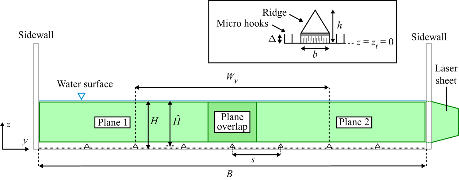
Figure 2. Schematic of the channel cross-section and ridge geometry.
Table 1. Experimental and analysis parameters:  $s$ is ridge spacing,
  $H$ is maximum flow depth,
  $\hat {H}$ is mean flow depth,
  $\varDelta = 1.1$ mm is the height of the cylindrical hooks covering the bed (figure 2),
  $Q$ is flow rate,
  $U = Q/(B\hat {H})$ is bulk flow velocity,
  $B = 400$ mm is channel width,
  $u_* = \sqrt {g\hat {H}S_b}$ is shear velocity,
  $g$ is acceleration due to gravity,
  $S_b$ is bed slope,
  $Re = U\hat {H}/\nu$ is bulk Reynolds number,
  $\nu$ is kinematic viscosity,
  $H^+ = u_*\hat {H}/\nu$ is friction Reynolds number,
  $Fr = U/\sqrt {g\hat {H}}$ is Froude number,
  $f_H = 8u_*^2/U^2$ is Darcy–Weisbach friction factor and
  $W_y$ is the width of the domain used for calculating spatially averaged variables.

4. Results
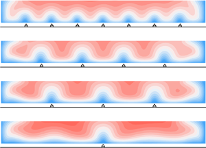
The time-averaged velocity fields for the different ridge spacings are shown in figure 3. The presence of depth-scale SC cells is clear for the s100 case ( $s = 2H$, table 1) while the SCs reduce in size as
  $s$ is reduced to
  $0.4H$ (s020, table 1). The rotation direction of these ridge-induced SCs is the same for all ridge spacings, and consistent with previous works (e.g. Nezu & Nakagawa Reference Nezu and Nakagawa1993; Vanderwel & Ganapathisubramani Reference Vanderwel and Ganapathisubramani2015; Hwang & Lee Reference Hwang and Lee2018). For the s000 case (without ridges), the central part of the flow away from the sidewalls is essentially homogeneous in the transverse direction and free of SCs. Distributions of the Reynolds stresses, turbulent kinetic energy and time-averaged vorticity for these flow conditions were presented in Zampiron et al. (Reference Zampiron, Cameron and Nikora2020a).

Figure 3. Contours of time-averaged streamwise velocity  $\bar {u}/u_*$ with
  $(\bar {v}/u_*,\bar {w}/u_*)$ vectors (shown in only half section for clarity). Horizontal lines mark ridge top (dash) and SC cell centre (dash-dot) elevations.
This paper complements that of Zampiron et al. (Reference Zampiron, Cameron and Nikora2020a) with analysis of the double-averaged momentum and energy conservation equations. The double-averaged quantities reported in this paper have been obtained using spatial-averaging domains (figure 1a) located in the central part of the flow cross-section where the effects of sidewall SCs are negligible (figure 3). The averaging domain width ( $W_y$) was selected to be an integer multiple of the ridge spacing (table 1) and was found to be adequate for approximating the studied cases as uniform two-dimensional double-averaged flows. Indeed, the data show that the transverse gradients of the double-averaged variables and double-averaged transverse and vertical velocities closely approach zero (i.e.
  $\partial \langle \bar {\phantom {u}}\rangle /\partial y = \langle \bar {v}\rangle = \langle \bar {w}\rangle = 0$), simplifying momentum (2.1) and energy (2.8)–(2.10) balance considerations. The vertical size of the averaging domains (
 $W_z$) was 2.5 mm while their streamwise extent (
 $W_x$) was approximately 2 mm corresponding, respectively, to the effective height of the PIV interrogation regions and the light sheet thickness. As for the time-averaging period, the whole measurement duration of 2 h was used.
Distributions of the double-averaged streamwise velocity  $\langle \bar {u}\rangle$, terms in the double-averaged momentum conservation equation (2.1) and momentum fluxes are shown in figures 4 to 8. Distributions of the kinetic energy, terms in the kinetic energy balance equations (2.8)–(2.10) and energy fluxes are presented in figures 9 to 13. Flow quantities are plotted as functions of
  $z/\varDelta$ and
  $z/H$ which are typically used in considerations of rough-bed OCFs. In addition, however, a third normalisation of
  $z$, i.e.
  $(z-d)/s$, is also used. This normalisation accounts for the ridge spacing and the SC ‘displacement height’
  $d$, and stems from Zampiron et al. (Reference Zampiron, Cameron and Nikora2020a) where the elevations of SC cell centres were seen to scale linearly with
  $s$ as
  $z_{sc} = d+0.21s$ (
 $d = 4.6$ mm) for a range of
  $s/H$ between 0.4 and 2.0. Using this normalisation, SC cell centre elevations (marked by dash-dot lines in figures 4–7, 9, 11, 13 and 15) are aligned at
  $(z-d)/s = 0.21$. Additionally, data presented in Zampiron et al. (Reference Zampiron, Cameron and Nikora2020a) showed that the strength of SCs in terms of time-averaged vertical and transverse velocities was approximately constant over a range of ridge spacings, while the size of the SCs scaled in proportion to
  $s$. This suggests that the magnitudes of dispersive momentum and energy fluxes are likely to be only weakly (if at all) dependent on
  $s$, while their vertical gradients, i.e. transport terms, should have similar magnitudes after multiplying by
  $s$. We use
  $z/\varDelta$,
  $z/H$, and
  $(z-d)/s$ scalings throughout the paper. Quantities involving vertical derivatives are made non-dimensional with
  $H$ for plots as functions
  $z/H$ which is conventional for flows over homogeneous beds, and by multiplying with
  $s$ for plots as functions of
  $(z-d)/s$ as justified above.

Figure 4. Double-averaged streamwise velocity and velocity gradient as functions of  $z/H$ and
  $z/\varDelta$ (a,c,e) and
  $(z-d)/s$ (b,d,f). The dotted line in (a) shows
  $\langle \bar {u}\rangle /u_* = \kappa ^{-1}\ln ([z-d_L]/\varDelta )+A_\varDelta$ with
  $\kappa = 0.41$,
  ${d_L = 1.1}$ mm and
  $A_{\varDelta } = 5.5$. Vertical lines mark ridge tops (dash), SC cell centres (dash-dot) and
  $z = 0$ (solid, i.e. increasing
  $s$ from left to right).
4.1. Mean velocity distributions, momentum balance and momentum fluxes
4.1.1. Mean velocity distributions
In figure 4, distributions of the double-averaged streamwise velocity  $\langle \bar {u}\rangle$ and its gradient
  $\partial {\langle \bar {u}\rangle }/\partial {z}$ are presented. Three distinct flow ranges can be identified: (i) a near-bed range where the velocity
  $\langle \bar {u}\rangle /u_*$ and its gradient
  $(\partial {\langle \bar {u}\rangle }/\partial {z})\varDelta /u_*$ scale with
  $z/\varDelta$ irrespective of the ridge spacing (figure 4a,e); (ii) an intermediate range around SC cell centres where
  $(\langle \bar {u}\rangle -\langle \bar {u}\rangle (z_{sc}))/u_*$ and
  $(\partial {\langle \bar {u}\rangle }/\partial {z})s/u_*$ collapse when using
  $(z-d)/s$ (figure 4d,f); and (iii) a near-free-surface range where the velocity difference
  $(\langle \bar {u}\rangle _{max}-\langle \bar {u}\rangle )/u_*$ and the normalised velocity gradient
 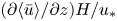 $(\partial {\langle \bar {u}\rangle }/\partial {z})H/u_*$ scale with
  $z/H$ irrespective of
  $s$ (figure 4c,e;
  $\langle \bar {u}\rangle _{max}$ is maximum velocity). Ranges (i) and (iii) are expected for two-dimensional flat-bed OCFs (where
  $\langle \bar {u}\rangle = \bar {u}$; e.g. Nezu & Nakagawa Reference Nezu and Nakagawa1993). This near-bed collapse of double-averaged velocity, and near-free-surface collapse of the velocity defect in highly three-dimensional flows with strong SCs suggest that away from the level of SC cell centres where absolute values of
  $\bar {w}$ are highest,
  $\varDelta$ and
  $H$ remain the dominant scales. In the near-bed range a logarithmic scaling of the double-averaged velocity in the form
  $\langle \bar {u}\rangle /u_* = \kappa ^{-1}\ln ([z-d_L]/\varDelta )+A_{\varDelta }$, with
  $\kappa = 0.41$,
  $d_L = 1.1$ mm and
  $A_{\varDelta } = 5.5$, appears to be approximately valid for all ridge spacings despite the presence of SCs (figure 4a). The extent of the intermediate range where
  $\partial {\langle \bar {u}\rangle }/\partial {z}$ is proportional to
  $s^{-1}$ is not sharply defined and appears to hold approximately over most of the measured elevations (figure 4d,f). The observed scaling, however, cannot continue to the bed level (
 $z = 0$) or the free surface, as the bed and water surface appear at different positions when the elevation is normalised as
  $(z-d)/s$. Therefore, departure of
  $(\langle \bar {u}\rangle -\langle \bar {u}\rangle (z_{sc}))/u_*$ and
  $(\partial {\langle \bar {u}\rangle }/\partial {z})s/u_*$ as functions of
  $(z-d)/s$ from a common trend can be expected approaching the bed and the free surface.
4.1.2. Momentum balance
For steady, uniform and two-dimensional double-averaged flows, the momentum conservation equation (2.1) in the streamwise direction reduces to
 \begin{equation} 0=\phi g S_b- \underbrace{{\frac{\partial \phi \langle \tilde{\bar{u}}\tilde{\bar{w}} \rangle}{\partial z}}}_{\text{$M_1$}} - \underbrace{{\frac{\partial \phi \langle \overline{u' w'} \rangle}{\partial z}}}_{\text{$M_2$}}+\underbrace{\frac{\partial}{\partial z} \left(\phi \nu \left\langle \overline{ \frac{\partial {u} }{\partial z}} \right\rangle\right)}_{\text{$M_3$}} - \frac{F_D}{\rho}. \end{equation}
The terms in (4.1) are presented in figure 5 as functions of  $z/\varDelta$,
  $z/H$ and
  $(z-d)/s$. As the drag term
  $F_D$ is zero above the ridge tops, the gravity term
  $\phi g S_b$ is locally balanced by the sum of the transport terms
  $-M_1$,
  $-M_2$ and
  $M_3$, i.e. associated with dispersive (due to SCs), turbulent and viscous stresses, respectively. The gravity term is constant for all
  $z$ above the ridge tops and is equal to 1.0 when normalised with
  $u_*^2/H$ (figure 5a). Due to the relatively high Reynolds number, the viscous momentum transport (
 $M_3$, figure 5g) is small compared to the transport due to turbulence (
 $-M_2$, figure 5e) and SCs (
 $-M_1$, figure 5c). The terms
  $-M_2$ and
  $-M_1$ counteract each other with local increases in one term balanced by local decreases in the other (and vice versa) such that their sum is approximately
  $-1.0$ over most of the flow depth when normalised with
  $u_*^2/H$. The contribution of SCs to the total momentum transport is significant, with
  $-M_1$ and
  $-M_2$ having comparable magnitudes. Distributions of
  $-M_1s/u_*^2$ have similar values at the SC cell centre elevation
  $(z-d)/s = 0.21$ for all
  $s$. The distributions when plotted as functions of
  $(z-d)/s$ (figure 5d) indicate that SCs contribute to a local loss of momentum above SC cell centres and a local gain of momentum in the region between ridge tops and SC cell centre elevations. The
  $-M_1s/u_*^2$ curves for different
  $s$ have similar shapes, but do not collapse precisely onto a common trend. This likely reflects a scale effect involving interactions between the SCs, the ridge geometry and the free surface. At small
  $s$ the SC cells are only slightly larger than the ridges themselves and the shape of the velocity contours, and subsequently the dispersive transport, will be impacted strongly by the ridge geometry. At the same time, the small SC cells will not feel the free surface or be modified significantly by it. At large
  $s$, in contrast, the larger SC cells are confined by the free surface but will not feel the shape of the ridge to the same extent. For this reason, we might expect to see closer collapse of the dispersive momentum transport distribution as the ridge relative submergence
  $H/h$ is increased.
4.1.3. Momentum fluxes
In this section, SC-induced dispersive  $\langle \tilde {\bar {u}}_i \tilde {\bar {u}}_j \rangle$ and spatially averaged turbulent
  $\langle \overline {u_i'u_j'}\rangle$ momentum flux distributions are explored. These momentum flux (or stress) terms appear in the double-averaged momentum balance equation (2.1). In a statistical sense, they essentially represent the variance or covariance of spatial
  $\tilde {\bar {u}}_i$ or turbulent
  $u_i'$ velocity fluctuations.
As shown in figure 3, the size of the SC cells scales with  $s$ and therefore it is reasonable to expect the dispersive fluxes
  $\langle \tilde {\bar {u}}_i \tilde {\bar {u}}_j \rangle$ to scale as functions of
  $(z-d)/s$ rather than
  $z/H$ or
  $z/\varDelta$. Indeed with this scaling of the vertical coordinate, the normalised streamwise
  $\langle \tilde {\bar {u}}\tilde {\bar {u}}\rangle /u_*^2$ and vertical
  $\langle \tilde {\bar {w}}\tilde {\bar {w}}\rangle /u_*^2$ normal stresses exhibit a similar trend for all spacings, attaining maximum values near the elevations of SC cell centres (figure 6b,f). The magnitude of the dispersive fluxes depends only weakly on
  $s$, which as noted in § 4.1.2 may be dependent on the ridge relative submergence
  $H/h$. Streamwise velocity spatial fluctuations
  $\tilde {\bar {u}}$ are strongly correlated with vertical velocity spatial fluctuations
  $\tilde {\bar {w}}$ such that
  $\langle \tilde {\bar {u}} \tilde {\bar {w}} \rangle \approx \langle \tilde {\bar {u}}\tilde {\bar {u}}\rangle ^{0.5}\langle \tilde {\bar {w}}\tilde {\bar {w}}\rangle ^{0.5}$, i.e. the correlation coefficient between
  $\tilde {\bar {u}}$ and
  $\tilde {\bar {w}}$ is
  ${\approx }1$. The normalised dispersive shear stress
  $-\langle \tilde {\bar {u}}\tilde {\bar {w}}\rangle /u_*^2$ attains a maximum value near the elevation of SC cell centres (figure 6h). The shape of the
  $\langle \tilde {\bar {u}}\tilde {\bar {u}}\rangle$,
  $\langle \tilde {\bar {w}}\tilde {\bar {w}}\rangle$ and
  $-\langle \tilde {\bar {u}}\tilde {\bar {w}}\rangle$ distributions confirms that momentum exchange due to SCs is largest near the SC cell centres where the magnitude of the local time-averaged vertical velocity is highest (figure 3). The location of the maximum dispersive stress contribution shifts slightly below the SC centre elevation as
  $s/H$ is reduced, likely due to the size of the SCs becoming comparable to the size of the ridges (i.e. decreased separation of scales of the ridges and SCs). A similar trend can be seen in the
  $\langle \tilde {\bar {u}}\tilde {\bar {u}}\rangle /u_*^2$ distribution. The maximum value of
  $-\langle \tilde {\bar {u}}\tilde {\bar {w}}\rangle /u_*^2$ of 0.3 is slightly larger than the
  ${\approx }0.25u_*^2$ reported by Vanderwel et al. (Reference Vanderwel, Stroh, Kriegseis, Frohnapfel and Ganapathisubramani2019) for boundary layer flows over rectangular-shaped ridges. Distributions of
  $\langle \tilde {\bar {v}}\tilde {\bar {v}}\rangle /u_*^2$ significantly differ from those of
  $\langle \tilde {\bar {u}}\tilde {\bar {u}}\rangle /u_*^2$ and
  $\langle \tilde {\bar {w}}\tilde {\bar {w}}\rangle /u_*^2$, presenting maximum values near the top and bottom boundaries of SC cells and being approximately zero at the SC cell centres (figure 6d). This reflects the distributions of
  $\bar {v}$ (figure 3), the magnitude of which is highest in the lower and upper parts of the SC cells.

Figure 6. Normal components of the dispersive momentum fluxes (a–f) and dispersive shear stress (g,h). Symbols and vertical lines are defined in figure 4.
The data show that turbulent velocity fluctuations  $u_i'$ are generally attenuated by the ridge-induced SCs as seen in the normalised distributions of the turbulent momentum fluxes
  $\langle \overline {u_i'u_j'}\rangle$ (figure 7). Much of the reduction of
  $\langle \overline {u'u'}\rangle$ (figure 7a) is associated with the suppression of large-scale turbulence structures, particularly VLSMs, by the SCs (Zampiron et al. Reference Zampiron, Cameron and Nikora2020a). The data of
  $\langle \overline {w'w'}\rangle$ for all studied values of
  $s$ closely collapse near the water surface (figure 7e), suggesting that this flow region is only weakly influenced by ridge-induced SCs, at least in a double-averaging sense. The spanwise turbulent variance
  $\langle \overline {v'v'}\rangle$ (figure 7c) appears to be increased/decreased at different elevations relative to s000 due to the interplay between SCs and turbulence. Local reductions in the normalised Reynolds stress
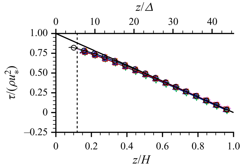
  $-\langle \overline {u'w'}\rangle /u_*^2$ (figure 7g) compared to the no-ridge case (s000) are balanced by local increases in the dispersive stress
  $-\langle \tilde {\bar {u}}\tilde {\bar {w}}\rangle /u_*^2$ (figure 6g) such that the fluid stress above the roughness tops (where
  $\phi = 1$ and
  $F_D = 0$) is equal to
  $gS_b(z_{ws}-z)/u_*^2$ as indicated by (2.4) and verified in figure 8. The slight deviation of the measured stress below the expected linear distribution near the bed is a known effect of the limited spatial resolution of the PIV measurements (e.g. Atkinson et al. Reference Atkinson, Buchmann, Amili and Soria2014). In all cases, the normalised viscous stress contribution
  $\nu \langle \overline {\partial {u}/\partial {z}}\rangle /u_*^2$ was less than 0.03 due to the relatively high Reynolds number. The drag term
  $\int _z^{z_{ws}}{F_D}\,\text {d}z$ appears only below the ridge tops, and is therefore not resolved by the current measurements.

Figure 7. Normal components of the spatially averaged turbulent momentum fluxes (a–f) and spatially averaged turbulent shear stress (g,h). Symbols and vertical lines are defined in figure 4.


4.2. Kinetic energy distributions, balance and fluxes
4.2.1. Kinetic energy distributions
The DMKE ( $\frac {1}{2} \langle \bar {u}_i\rangle \langle \bar {u}_i\rangle$), DKE (
 $\frac {1}{2} \langle \tilde {\bar {u}}_i \tilde {\bar {u}}_i \rangle$) and SATKE (
 $\frac {1}{2} \langle \overline {u'_iu'_i} \rangle$) are shown in figure 9 as functions of
  $z/\varDelta$,
  $z/H$ and
  $(z-d)/s$. The DMKE (figure 9a,b) distributions follow trends similar to those of the streamwise velocity reported in figure 4. This similarity could be expected as the DMKE in these cases is equal to half the square of
  $\langle \bar {u}\rangle /u_*$ since
  $\langle \bar {v}\rangle$ and
  $\langle \bar {w}\rangle$ are near zero for the selected spatial-averaging domain. The DKE and SATKE profiles reflect distributions of their constituent normal stresses reported in figures 6 and 7. The largest DKE for the s100 case is
  ${\approx }0.7u_*^2$ which is about 50 % of the SATKE at the same level (i.e. at the elevation of SC cell centres; figure 9d,f). For s020, the peak ratio of DKE to SATKE reduces to approximately 20 %–25 %, still remaining significant. These estimates show that the contribution of the SCs to the flow kinetic energy is comparable to that provided by turbulence, and therefore cannot be neglected. Compared to the no-ridge case (s000), the SATKE is noticeably reduced for all cases with ridges on the bed (
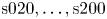 $\textrm {s}020,\ldots ,\textrm {s}200$; figure 9e). As was noted in § 4.1.3 for the streamwise velocity variance, this turbulent kinetic energy reduction likely reflects the suppression of VLSMs by the SCs as was noted in the velocity spectra by Zampiron et al. (Reference Zampiron, Cameron and Nikora2020a).

Figure 9. Distributions of DMKE (a,b), DKE (c,d) and SATKE (e,f). Symbols and vertical lines are defined in figure 4.
4.2.2. Kinetic energy balance
For the case of steady, uniform and two-dimensional double-averaged flow ( $\partial \langle \bar {\phantom {\varTheta }}\rangle /\partial {t} = \partial \langle \bar {\phantom {\varTheta }}\rangle /\partial {x} = \partial \langle \bar {\phantom {\varTheta }}\rangle /\partial {y} = \langle \bar {v}\rangle = \langle \bar {w}\rangle = 0$), (2.8)–(2.10) reduce to
 \begin{align} \text{DMKE}:\;&0=G+I_1+I_2+I_4-I_5\phantom{{}+{}I_6}\:-T_{2\phantom{2}}-T_{3\phantom{3}}\phantom{{}-{}T_{14}^{**}}+T_{5\phantom{0}}\:-D_1-D_2 , \end{align}
 \begin{align} \text{DKE}:\;&0=\phantom{G}{}-{}I_1\phantom{{}+{}I_2}-I_4+I_5+I_6\:-T_{7\phantom{2}}-T_{8\phantom{3}}-T_{9\phantom{4}}^{*\phantom{*}}+T_{10}\:-D_2-D_3 , \end{align}
 \begin{align} \text{SATKE}:\;&0=\phantom{G}\underbrace{\phantom{\;+{}{I_1}}-I_2\phantom{\:+{}I_4\:-{}I_5}-I_6}_{\substack{\text{Interbudget}\\\text{exchange}}}\underbrace{\;-\:T_{12}-T_{13}-T_{14}^{**}+T_{15}}_{\text{Transport}}\underbrace{\;-\:D_4^{**}\phantom{{}-{}D_3}}_{\text{Dissipation}} . \end{align}
Distributions of the terms (normalised by  $u_*^3/H$) of (4.2) to (4.4) are presented in figure 10 as functions of
  $z/H$ and
  $z/\varDelta$. Figure 11 shows the vertical distribution of the same terms (normalised by
  $u_*^3/s$) as functions of
  $(z-d)/s$. The dissipation to heat terms
  $-D_1$ and
  $-D_3$ in the respective DMKE and DKE budgets were found to be negligible and are therefore excluded from the figures. Similarly, the viscous transport terms
  $T_5$,
  $T_{10}$ and
  $T_{15}$ were found to be small in the above-ridge-top region compared to the other transport terms and are also not shown. The pressure transport
  $-T_{14}$ and dissipation to heat
  $-D_4$ terms (marked by double asterisk in (4.4)) could not be calculated from the available data due to the lack of pressure measurements and insufficient spatial resolution of the PIV system, respectively. The pressure transport term
  $-T_9$ in the DKE budget (marked by a single asterisk) could not be measured directly and therefore it was estimated as a residual as all other terms in (4.3) were directly measured. The terms
  $D_2$,
  $I_4$ and
  $I_5$ are non-zero below the ridge tops only and therefore are not included into consideration due to the lack of measurements in that flow region.


Equations (2.8) and (4.2) indicate that the energy is supplied to the DMKE budget by gravity at a rate  $G = \phi gS_b\langle \bar {u}\rangle$. From there it is distributed to the DKE budget through the interbudget (DMKE–DKE) exchange terms
  $I_1$,
  $I_4$ and
  $-I_5$, and to the SATKE budget through the interbudget (DMKE–SATKE) exchange term
  $I_2$. Figure 10 shows that in the near-free-surface region the rate of supply of DMKE (
 $GH/u_*^3$; figure 10a) exceeds the loss to DKE and SATKE (
 $I_1H/u_*^3$ and
  $I_2H/u_*^3$, respectively; figure 10b,e), while near the bed the opposite occurs. Therefore, it can be deduced that the role of the transport terms due to SCs (
 $-T_2$; figure 10h) and due to turbulence (
 $-T_3$; figure 10k) is to redistribute DMKE from the excess supply region near the free surface to the excess loss region near the bed. The two terms counterbalance each other to some extent, with local increases/decreases of
  $-T_2$ relative to the no-ridge s000 case balanced by local reductions/enhancements in
  $-T_3$. Figure 11(h) indicates that
  $-T_2$ is generally a loss above SC cell centres and a gain below this level. Neither
  $-T_2$,
  $-T_3$ nor
  $I_2$ scale exclusively with
  $s$ or
  $H$ and in general are functions of the relative ridge spacing
  $s/H$. It follows from observations in §§ 4.1.1 and 4.1.3 of
  $(\partial {\langle \bar {u}\rangle }/\partial {z})s/u_*$ and
  $\langle \tilde {\bar {u}}\tilde {\bar {w}}\rangle /u_*^2$ collapsing as functions of
  $(z-d)/s$, that
  $I_1$ should follow a similar scaling. Indeed, figure 11(b) exhibits a close data collapse and thus the rate at which energy is supplied to the DKE budget (
 $I_1$) is inversely proportional to the ridge spacing
  $s$, i.e. the SC cell size.
Within the DKE budget, the gain from the DMKE budget through  $-I_1$ is counterbalanced by the loss to the SATKE budget through
  $I_6$ (figures 10c,f and 11c,f). The DMKE–DKE interbudget exchange terms
  $I_5$ (due to the action of viscous drag) and
  $-I_4$ (due to the action of pressure drag) are expected to provide additional contributions to the production of DKE below the ridge tops and below the tops of the hook roughness, respectively. The difference between
  $I_1$ and
  $I_6$ above the ridge tops is balanced by the transport terms
  $-T_7$,
  $-T_8$ and
  $-T_9^*$, whose net effect is to redistribute DKE from the excess production zone below the SC cell centres to elevations just above SC cell centres (figure 11i,l,n) where the loss to the SATKE budget exceeds the gain from the DMKE budget. The net transport of DKE is dominated by
  $-T_8$ which appears to scale as a function of
  $(z-d)/s$, although the magnitude of
  $-T_8s/u_*^3$ weakly depends on the relative ridge spacing
  $s/H$.
At the elevation of the SC cell centres, the production rate of SATKE via the DKE budget ( $-I_6$) reaches approximately double the production rate via the DMKE budget (
 $-I_2$) for the s100 ridge spacing (figure 11g,d). For the s020 case, the ratio of
  $-I_6$ to
  $-I_2$ reduces to approximately 50 %. Both
  $-I_2$ and
  $-I_6$ are gains for the SATKE budget within the whole measured flow region (from the ridge tops to the water surface). The transport terms
  $-T_{12}$ and
  $-T_{13}$ (figure 10j,m) are small compared to the interbudget exchange terms
  $-I_2$ and
  $-I_6$ (figure 10d,g) near the bed suggesting an approximate balance between production and dissipation which is typical for the flow region just above the roughness tops of rough-bed OCFs (e.g. Nezu & Nakagawa Reference Nezu and Nakagawa1993; Mignot et al. Reference Mignot, Barthélemy and Hurther2009; Yuan & Piomelli Reference Yuan and Piomelli2014). Approaching the free surface, the resulting effect of the resolved transport terms (i.e.
  $-T_{12}$,
  $-T_{13}$,
  $T_{15}$) is a ‘gain’ indicating that dissipation of SATKE to heat via
  $-D_4$ (not measured) likely exceeds the production rate at these elevations. Transport of SATKE due to SCs (
 $-T_{12}$; figure 11j) appears to scale as a function of
  $(z-d)/s$ with
  $-T_{12}/u_*^3$ being inversely proportional to
  $s$. Near SC cell centres, the magnitude of
  $-T_{12}$ is comparable to
  $-T_{13}$ (figure 11m), in contrast to rough-wall flows without SCs where Mignot et al. (Reference Mignot, Barthélemy and Hurther2009) found the transport due to mean flow heterogeneity (
 $-T_{12}$) to be negligible. Also important to note is a shift of the
  $-T_{13}H/u_*^3$ distributions for s020 and s025 towards lower values compared to s000 (figure 10m) at
  $z/H>0.4$, the region of homogeneous flow above the SCs (figure 3). This may be explained by the lack of VLSMs in the whole flow despite the small SCs confined to the near-bed region (Zampiron et al. Reference Zampiron, Cameron and Nikora2020a).
4.2.3. Kinetic energy fluxes
Energy fluxes ( $E_n$) are presented in figure 12 as functions of
  $z/H$ and
  $z/\varDelta$ and in figure 13 as functions of
  $(z-d)/s$ (all the terms are explicitly defined in the figure caption). Only energy fluxes in the vertical direction are considered as they are the sole contributors to the energy transport if the double-averaged flow is uniform and two-dimensional. Vertical energy fluxes are closely related to the energy transport terms in the kinetic energy conservation equations (2.8)–(2.10) (i.e. the transport terms are the derivatives of the vertical energy fluxes with respect to
  $z$) and therefore their analysis complements the results presented in the previous section. For clarity, the subscript of each term
  $E_n$ matches that of the corresponding transport term
  $T_n$ (2.8)–(2.10).

Figure 12. Distributions of energy fluxes as functions of  $z/\varDelta$ and
  $z/H$: (a)
  $E_2 = \phi \langle \bar {u}_i \rangle \langle \tilde {\bar {u}}_i \tilde {\bar {w}} \rangle$; (b)
  $E_7 = \phi \langle \tilde {\bar {u}}_i \tilde {\bar {u}}_i \tilde {\bar {w}} \rangle$; (c)
  $E_{12} = \phi \langle \overline {u'_iu'_i}\tilde {\bar {w}}\rangle$; (d)
  $E_3 = \phi \langle \bar {u}_i \rangle \langle \overline {u'_iw'} \rangle$; (e)
  $E_8 = \phi \langle \tilde {\bar {u}}_i \overline {u'_iw'} \rangle$; (f)
  $E_{13} = \phi \langle \overline {u'_iu'_iw'}\rangle$. Symbols and vertical lines are defined in figure 4.

Figure 13. Distributions of energy fluxes as functions of  $(z-d)/s$: (a)
  $E_2 = \phi \langle \bar {u}_i \rangle \langle \tilde {\bar {u}}_i \tilde {\bar {w}} \rangle$; (b)
  $E_7 = \phi \langle \tilde {\bar {u}}_i \tilde {\bar {u}}_i \tilde {\bar {w}} \rangle$; (c)
  $E_{12} = \phi \langle \overline {u'_iu'_i}\tilde {\bar {w}}\rangle$; (d)
  $E_3 = \phi \langle \bar {u}_i \rangle \langle \overline {u'_iw'} \rangle$; (e)
  $E_8 = \phi \langle \tilde {\bar {u}}_i \overline {u'_iw'} \rangle$; (f)
  $E_{13} = \phi \langle \overline {u'_iu'_iw'}\rangle$. Symbols and vertical lines are defined in figure 4.
Distributions of the energy fluxes associated with the SCs ( $E_2$,
  $E_7$,
  $E_8$ and
  $E_{12}$) have similar shapes for all
  $s$ when presented as functions of
  $(z-d)/s$ (figures 13a–c and 13e, respectively), with peak values found at elevations near SC cell centres and magnitudes that depend only weakly on
  $s/H$. Both DMKE flux terms (
 $E_2$ and
  $E_3$) are negative for all elevations indicating that DMKE is transported by SCs and turbulence towards the bed. In contrast, fluxes of DKE and SATKE are generally positive above the ridge tops (figure 12b,e,c,f), indicating upward fluxes of energy compensating the excess production of DKE and SATKE in the near-bed region.
Figure 12(f) indicates that the spatially averaged turbulent flux of the turbulent kinetic energy ( $E_{13}$) is significantly suppressed by the SCs, even at elevations above the SC cells for s020 and s025 (recall that these cells are located near the bed, with a significant flow region above them being free of SCs; figure 3), which explains the offset between
  $-T_{13}H/u_*^3$ distributions for s020, s025 and s000 (figure 10m). This effect likely relates to the suppression of VLSMs by the SCs identified by Zampiron et al. (Reference Zampiron, Cameron and Nikora2020a) and also observed when considering
  $\langle \overline {u'u'}\rangle$ in § 4.1.3 and
  $\frac {1}{2}\langle \overline {u'_iu'_i}\rangle$ in the previous section. Indeed, the lower values of
  $\langle \overline {u'u'}\rangle$ and
  $\frac {1}{2}\langle \overline {u'_iu'_i}\rangle$ in the outer flow region cannot be due to energy exchanges, as for
  $z/H>0.4$ distributions of
  $-I_2H/u_*^3$ and
  $-I_6H/u_*^3$ for s020 and s025 (i.e. above the SCs) collapse with that for s000 (figure 10d,g). For the no-ridge case (s000), the peak value of
  $E_{13}/u_*^3$ is 0.67 (figure 12f), quite close to the 0.66 reported for smooth-wall OCFs by López & García (Reference López and García1999), but slightly smaller than the 0.76 reported for rough-wall OCFs by Hurther, Lemmin & Terray (Reference Hurther, Lemmin and Terray2007).
4.3. Origin of secondary currents
The mechanisms that generate SCs in flows over spanwise heterogeneous roughness have been explored by a number of researchers (e.g. Einstein & Li Reference Einstein and Li1958; Hinze Reference Hinze1967, Reference Hinze1973; Nezu & Nakagawa Reference Nezu and Nakagawa1984, Reference Nezu and Nakagawa1993; Nikora & Roy Reference Nikora and Roy2012; Anderson et al. Reference Anderson, Barros, Christensen and Awasthi2015; Hwang & Lee Reference Hwang and Lee2018). Regardless of the chosen approach (i.e. analysis of time-averaged momentum, time-averaged streamwise vorticity or energy balance equations), the common understanding is that the emergence of such SCs is due to turbulence anisotropy introduced by the wall-surface heterogeneities. In this section, we further investigate the issue using double-averaged conservation equations for the dispersive normal stresses (i.e. stresses generated by SCs).
Balance equations for  $\langle \tilde {\bar {u}}\tilde {\bar {u}}\rangle$,
  $\langle \tilde {\bar {v}}\tilde {\bar {v}}\rangle$ and
  $\langle \tilde {\bar {w}}\tilde {\bar {w}}\rangle$ stem from the conservation equation for the dispersive stress tensor (A2). For steady
  $\partial {\langle \bar {\phantom {\varTheta }}\rangle }/\partial {t} = 0$, uniform
  $\partial \langle \bar {\phantom {\varTheta }}\rangle /\partial {x} = 0$ and two-dimensional
  $\langle \bar {v}\rangle = \langle \bar {w}\rangle = \partial \langle \bar {\phantom {\varTheta }}\rangle /\partial {y} = 0$ flow, the conservation equation for
  $\langle \tilde {\bar {u}}\tilde {\bar {u}}\rangle$ is
 \begin{align} &\left.\begin{aligned} 0 & ={-}\underbrace{2\phi \langle \tilde{\bar{u}} \tilde{\bar{w}} \rangle \frac{\partial \langle \bar{u}\rangle}{\partial z}}_{I_{1u}}+\underbrace{2\phi \left\langle \overline{u'u_j'} \frac{\partial \tilde{\bar{u}}}{\partial x_j} \right\rangle}_{I_{6u}}\\ \phantom{0} & \quad-\underbrace{2\frac{\langle \bar{u} \rangle }{\rho V_0}\iint\limits_{S_{int}} \bar{p}m_1\,\text{d}S}_{I_{4u}}+\underbrace{2 \frac{\langle \bar{u} \rangle}{V_0} \iint\limits_{S_{int}}\nu \frac{\partial \bar{u}}{\partial x_j}m_j\,\text{d}S}_{I_{5u}} \end{aligned}\notag\right\rbrace\begin{aligned}\text{Interbudget}\\ \text{exchange}\end{aligned}\nonumber\\ &\quad\left.\begin{aligned} \phantom{0} & +\underbrace{2\frac{\phi}{\rho}\left\langle\bar{p}\frac{\partial\bar{u}}{\partial x}\right \rangle}_{P_{1u}}\\ \end{aligned}\right\rbrace\text{Pressure strain rate}\nonumber\\ &\quad\left.\begin{aligned} \phantom{0} & -\underbrace{\frac{\partial \phi\langle \tilde{\bar{u}} \tilde{\bar{u}}\tilde{\bar{w}}\rangle}{\partial z}}_{T_{7u}}- \underbrace{2\frac{\partial \phi\langle \tilde{\bar{u}}\overline{u'w'} \rangle}{\partial z}}_{T_{8u}}+ \underbrace{2\nu\frac{\partial}{\partial z} \left(\phi \left\langle \tilde{\bar{u}} \frac{\partial \tilde{\bar{u}}}{\partial z} \right\rangle \right)}_{T_{10u}}\\ \end{aligned}\right\rbrace\text{Transport}\nonumber\\ &\quad\left.\begin{aligned} \phantom{0} & -\underbrace{2\phi\nu \frac{\partial \langle \bar{u} \rangle}{\partial z} \left\langle \frac{\partial \tilde{\bar{u}}}{\partial z}\right\rangle}_{D_{2u}}- \underbrace{2\phi\nu \left\langle \frac{\partial \tilde{\bar{u}} }{\partial x_j} \frac{ \partial \tilde{\bar{u}} }{\partial x_j} \right\rangle}_{D_{3u}}\\ \end{aligned}\right\rbrace\text{Dissipation to heat,} \end{align}
the conservation equation for  $\langle \tilde {\bar {v}}\tilde {\bar {v}}\rangle$ is
 \begin{align} &\left.\begin{aligned} 0 & =\underbrace{2\phi \left\langle \overline{v'u'_j} \frac{\partial \tilde{\bar{v}}}{\partial x_j} \right\rangle}_{I_{6v}}\\ \end{aligned}\notag\right\rbrace\text{Interbudget exchange}\nonumber\\ &\quad\left.\begin{aligned} \phantom{0} & +\underbrace{2\frac{\phi}{\rho}\left\langle\bar{p}\frac{\partial\bar{v}}{\partial y} \right\rangle}_{P_{1v}}\\ \end{aligned}\right\rbrace\text{Pressure strain rate}\nonumber\\ &\quad\left.\begin{aligned} \phantom{0} & -\underbrace{\frac{\partial\phi\langle\tilde{\bar{v}}\tilde{\bar{v}}\tilde{\bar{w}}\rangle}{ \partial z}}_{T_{7v}}-\underbrace{2\frac{\partial \phi\langle\tilde{\bar{v}}\overline{v'w'} \rangle}{ \partial z}}_{T_{8v}}+\underbrace{2\nu\frac{\partial}{\partial z} \left(\phi \left\langle \tilde{\bar{v}} \frac{\partial \tilde{\bar{v}}}{\partial z} \right\rangle \right)}_{T_{10v}}\\ \end{aligned}\right\rbrace\text{Transport}\nonumber\\ &\quad\left.\begin{aligned} \phantom{0} & -\underbrace{2\phi\nu \left\langle \frac{\partial \tilde{\bar{v}} }{\partial x_j} \frac{\partial \tilde{\bar{v}} }{\partial x_j} \right\rangle}_{D_{3v}}\\ \end{aligned}\right\rbrace\text{Dissipation to heat} \end{align}
and, finally, the conservation equation for  $\langle \tilde {\bar {w}}\tilde {\bar {w}}\rangle$ is
 \begin{align} &\left.\begin{aligned} 0 & =\underbrace{2\phi \left\langle \overline{w'u'_j} \frac{\partial \tilde{\bar{w}}}{\partial x_j} \right\rangle}_{I_{6w}}\\ \end{aligned}\notag\right\rbrace\text{Interbudget exchange}\nonumber\\ &\quad\left.\begin{aligned} \phantom{0} & +\underbrace{2\frac{\phi}{\rho}\left\langle\bar{p}\frac{\partial\bar{w}}{\partial z} \right\rangle}_{P_{1w}}\\ \end{aligned}\right\rbrace\text{Pressure strain rate}\nonumber\\ &\quad\left.\begin{aligned} \phantom{0} & -\underbrace{\frac{\partial\phi\langle\tilde{\bar{w}}\tilde{\bar{w}}\tilde{\bar{w}} \rangle}{\partial z}}_{T_{7w}}-\underbrace{2\frac{\partial \phi\langle \tilde{\bar{w}}\overline{w'w'} \rangle}{\partial z}}_{T_{8w}}\\ & -\underbrace{\frac{2}{\rho}\frac{\partial\phi\langle\tilde{\bar{p}}\tilde{\bar{w}}\rangle}{\partial z}}_{T_{9w}}+\underbrace{2\nu\frac{\partial}{\partial z} \left(\phi \left\langle \tilde{\bar{w}} \frac{\partial \tilde{\bar{w}}}{\partial z} \right\rangle \right)}_{T_{10w}}\\ \end{aligned}\right\rbrace\text{Transport}\nonumber\\ &\quad\left.\begin{aligned} \phantom{0} & -\underbrace{2\phi\nu \left\langle \frac{\partial \tilde{\bar{w}} }{\partial x_j} \frac{\partial \tilde{\bar{w}} }{\partial x_j} \right\rangle}_{D_{3w}}\\ \end{aligned}\right\rbrace\text{Dissipation to heat.} \end{align}
The terms in (4.5)–(4.7) are subsets of those in the DKE balance (2.9), e.g.  $0.5(I_{6u}+I_{6v}+I_{6w}) = I_6$. Of particular interest are the pressure-strain rate terms (
 $P_{1u}$,
  $P_{1v}$ and
  $P_{1w}$), which following the mass conservation equation sum to zero, i.e.
 \begin{equation} P_{1u}+P_{1v}+P_{1w} = 2\frac{\phi}{\rho}\left\langle\bar{p}\left(\frac{\partial\bar{u}}{\partial x}+\frac{\partial\bar{v}}{\partial y}+\frac{\partial\bar{w}}{\partial z}\right)\right\rangle=0, \end{equation}
and therefore do not appear in the DKE budget (2.9). The roles of  $P_{1u}$,
  $P_{1v}$ and
  $P_{1w}$ are to exchange energy between the
  $\langle \tilde {\bar {u}}\tilde {\bar {u}}\rangle$,
  $\langle \tilde {\bar {v}}\widetilde {\bar {v}}\rangle$ and
  $\langle \tilde {\bar {w}}\tilde {\bar {w}}\rangle$ budgets. For the specific case of two-dimensional streamwise ridges (as in our study)
  $P_{1u} = 0$ as
  $\partial \bar {u}/\partial x = 0$. Equation (4.8) then reduces to
  $P_{1v} = -P_{1w}$ and thus there is no exchange of energy between the streamwise (
 $\langle \tilde {\bar {u}}\tilde {\bar {u}}\rangle$) and the secondary (
 $\langle \tilde {\bar {v}}\tilde {\bar {v}}\rangle$ and
  $\langle \tilde {\bar {w}}\tilde {\bar {w}}\rangle$) components of DKE. Considering the budgets for
  $\langle \tilde {\bar {v}}\tilde {\bar {v}}\rangle$ (4.6) and
  $\langle \tilde {\bar {w}}\tilde {\bar {w}}\rangle$ (4.7) which contain the energy of the SC cellular vortices, the only possible terms to provide a net energy supply to the SCs are therefore
  $I_{6v}$ and
  $I_{6w}$. These terms have counterparts with opposite sign in the budgets for
  $\langle \overline {v'v'}\rangle$ and
  $\langle \overline {w'w'}\rangle$ (A3). Equations (4.6) and (4.7) therefore show explicitly that energy must be supplied to the secondary motions via the transverse and vertical components of the turbulent kinetic energy. Figure 14 summarises the energy exchanges that generate and sustain SCs. Energy is initially supplied to the streamwise component of the double mean flow where it is distributed to the streamwise turbulent fluctuations both directly and via the spatial fluctuations of the time-averaged streamwise velocity. Pressure fluctuations distribute energy from the streamwise turbulent fluctuations to the vertical and transverse turbulent fluctuations which ultimately exchange energy with the SCs. Figure 14 indicates that SCs cannot form in laminar flows over streamwise ridges.

Figure 14. Energy exchanges that generate and sustain SCs in flows over streamwise ridges, where  $P_{2u} = 2\phi \langle \overline {p'(\partial u'/\partial x)}\rangle /\rho$,
  $P_{2v} = 2\phi \langle \overline {p'(\partial v'/\partial y)}\rangle /\rho$,
 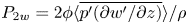 $P_{2w} = 2\phi \langle \overline {p'(\partial w'/\partial z)}\rangle /\rho$ and
 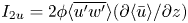 $I_{2u} = 2\phi \langle \overline {u'w'} \rangle (\partial \langle \bar {u}\rangle /\partial z)$. Other terms are defined in (4.5)–(4.7).
Our data for the  $\langle \tilde {\bar {v}}\tilde {\bar {v}}\rangle +\langle \tilde {\bar {w}}\tilde {\bar {w}}\rangle$ budget show that the net energy exchange is negative above the ridge tops (figure 15a), indicating loss of energy from SCs to turbulence. We know that
  $I_{6v}+I_{6w}$ when integrated over the flow depth must be greater than zero to balance the losses to heat through
  $D_{3v}$ and
  $D_{3w}$. Therefore, we can infer from figure 15(a,b) that
  $I_{6v}+I_{6w}$ must be strongly positive in the region below the ridge tops where data are not yet available. We therefore conclude from our analysis of the dispersive stress balance equations that SCs are generated and sustained by harvesting the energy of transverse and vertical turbulent velocity fluctuations in the near-bed region.


5. Conclusions
Ridge-induced SCs and their interactions with turbulence in OCFs were explored by assessing the distributions of terms in the double-averaged momentum and energy conservation equations. The data obtained from stereoscopic PIV measurements indicate that near the elevation of SC cell centres, the vertical gradient of the double-averaged streamwise velocity is inversely proportional to the transverse spacing ( $s$) of longitudinal ridges on the bed. This new scaling for the streamwise velocity appears at intermediate elevations between traditional rough-bed OCF regions near the bed and near the free surface. Distributions of the momentum and energy fluxes associated with the SCs were found to collapse reasonably well if presented as functions of the relative elevation
  $(z-d)/s$ with magnitudes generally independent of
  $s$, where
  $d$ is a ‘SC displacement height’ that aligns the elevations of SC cell centres for different
  $s$.
$s$.
Analysis of the budget equations for DMKE, DKE and SATKE components indicates that energy is supplied to the DMKE budget via a gravity source term and finally is dissipated to heat predominately within the SATKE budget. There is very little direct dissipation to heat within the DMKE and DKE budgets. The energy is supplied to turbulence directly from the DMKE budget as well as through a second production term via the DKE budget associated with SCs. At the elevation of SC cell centres, the ratio of the production rate of SATKE via the DKE budget to the production rate via the DMKE budget changes from  ${\approx }2$ for
  $s/H = 2$ (depth-scale SCs) to
  ${\approx }0.5$ for
  $s/H = 0.4$ (small near-bed SCs).
The overall effect of the SCs was to reduce the turbulent energy, likely due to the suppression of VLSMs (Zampiron et al. Reference Zampiron, Cameron and Nikora2020a). This reduction can be observed also for small ridge spacings, where SCs are confined near the bed and the overlying flow is homogeneous in the spanwise direction. In these cases, the data suggest that such a reduction is due to the decrease of turbulent transport of energy from near the bed towards the outer flow.
Study of the conservation equations for the dispersive stresses shows that the energy supplied to SCs does not come directly from the double-mean flow, or from spatial fluctuations of the streamwise velocity. Instead, the only source term in the dispersive stress budget is via exchange of energy with the turbulent flow field. The data imply that the energy to generate and sustain SC motions is supplied by transverse and vertical turbulent fluctuations, predominantly in the near-bed region.
Further data are required to clarify: the behaviour of the SCs at very small ridge spacings ( $s/H<0.4$); the role of ridge geometry (e.g. different ridge cross-sectional shapes such as squares, rectangles and semicircles); and the role of the ridge size (e.g. ridge height to flow depth ratio).
Acknowledgements
Discussions with I. Marusic (University of Melbourne) and B. Ganapathisubramani (University of Southampton) are greatly appreciated.
Funding
Financial support was provided by the EPSRC/UK grant ‘Bed friction in rough-bed free-surface flows: a theoretical framework, roughness regimes, and quantification’ (grant EP/K041088/1).
Declaration of interests
The authors report no conflict of interest.
Appendix A. Conservation equations for the fluid stresses
Papadopoulos et al. (Reference Papadopoulos, Nikora, Cameron, Stewart and Gibbins2020) derived double-averaged balance equations for the fluid stresses for the case of OCFs over mobile rough beds. For fixed beds, the conservation equation for the double-mean stresses reduces to
 \begin{align} &\left.\begin{aligned} \frac{\partial\phi\langle\bar{u}_i\rangle\langle\bar{u}_k\rangle}{\partial t} & =\\ \end{aligned}\notag\right\rbrace\text{Time rate of change}\nonumber\\ &\left.\begin{aligned} \phantom{\frac{\partial\phi\langle\bar{u}_i\rangle\langle\bar{u}_k\rangle}{\partial t}} & + \phi\left(\langle\bar{u}_i\rangle g_k+\langle\bar{u}_k\rangle g_i\right)\\ \end{aligned}\right\rbrace\text{Source}\nonumber\\ &\left.\begin{aligned} \phantom{\frac{\partial\phi\langle\bar{u}_i\rangle\langle\bar{u}_k\rangle}{\partial t}} & +\phi\left( \langle \tilde{\bar{u}}_i\tilde{\bar{u}}_j\rangle\frac{\partial\langle\bar{u}_k\rangle}{\partial x_j} + \langle\tilde{\bar{u}}_k\tilde{\bar{u}}_j\rangle\frac{\partial\langle\bar{u}_i\rangle}{\partial x_j} \right)\\ & +\phi\left(\langle\overline{u'_iu'_j}\rangle\frac{\partial\langle\bar{u}_k\rangle}{ \partial x_j}+\langle\overline{u'_ku'_j}\rangle\frac{\partial\langle\bar{u}_i\rangle}{\partial x_j}\right)\\ & +\frac{\phi}{\rho}\langle\bar{p}\rangle\left(\frac{\partial\langle\bar{u}_k\rangle}{\partial x_i}+\frac{\partial\langle\bar{u}_i\rangle}{\partial x_k}\right)\\ & +\frac{\langle\bar{u}_k\rangle}{\rho V_0}\iint\limits_{S_{int}} \bar{p}m_i\,\text{d}S+\frac{\langle\bar{u}_i\rangle}{\rho V_0}\iint\limits_{S_{int}}\bar{p}m_k\,\text{d}S\\ & -\frac{\langle\bar{u}_k\rangle}{V_0}\iint\limits_{S_{int}}\nu\frac{\partial\bar{u}_i}{\partial x_j}m_j\, \text{d}S-\frac{\langle\bar{u}_i\rangle}{V_0}\iint\limits_{S_{int}}\nu\frac{\partial\bar{u}_k}{\partial x_j}m_j\,\text{d}S\\ \end{aligned}\right\rbrace\begin{aligned}\text{Interbudget}\\ \text{exchange}\end{aligned}\nonumber\\ &\left.\begin{aligned} \phantom{\frac{\partial\phi\langle\bar{u}_i\rangle\langle\bar{u}_k\rangle}{\partial t}} & - \frac{\partial\phi\langle\bar{u}_i\rangle\langle\bar{u}_k\rangle\langle\bar{u}_j\rangle}{ \partial x_j}-\frac{\partial\phi\left(\langle\bar{u}_k\rangle\langle\tilde{\bar{u}}_i\tilde{ \bar{u}}_j\rangle+\langle\bar{u}_i\rangle\langle\tilde{\bar{u}}_k\tilde{\bar{u}}_j\rangle\right)}{\partial x_j}\\ & -\frac{\partial\phi(\langle\bar{u}_k\rangle\langle\overline{u'_iu'_j}\rangle+\langle\bar{u}_i\rangle\langle\overline{u'_ku'_j}\rangle)}{\partial x_j}\\ & -\frac{1}{\rho}\frac{\partial\phi(\langle\bar{p}\rangle\langle\bar{u}_k\rangle\delta_{ij}+\langle\bar{p}\rangle\langle\bar{u}_i\rangle\delta_{kj})}{\partial x_j}\\ & +\nu\frac{\partial}{\partial x_j}\left(\langle\bar{u}_k\rangle\frac{\partial \phi\langle\bar{u}_i\rangle}{\partial x_j}+\langle\bar{u}_i\rangle\frac{\partial \phi\langle\bar{u}_k\rangle}{\partial x_j}\right) \end{aligned}\right\rbrace\text{Transport}\nonumber\\ &\left.\begin{aligned} \phantom{\frac{\partial\phi\langle\bar{u}_i\rangle\langle\bar{u}_k\rangle}{\partial t}} & - 2\phi\nu\frac{\partial\langle\bar{u}_i\rangle}{\partial x_j}\frac{\partial\langle\bar{u}_k\rangle}{\partial x_j}\\ & -\phi\nu\left(\frac{\partial\langle\bar{u}_i\rangle}{\partial x_j} \left\langle\frac{\partial \tilde{\bar{u}}_k}{\partial x_j}\right\rangle+ \frac{\partial\langle\bar{u}_k\rangle}{\partial x_j} \left\langle\frac{\partial \tilde{\bar{u}}_i}{\partial x_j}\right\rangle\right)\\ \end{aligned}\right\rbrace\begin{aligned}\text{Dissipation}\\ \text{to heat,}\end{aligned} \end{align}
the conservation equation for the dispersive stresses becomes
 \begin{align} &\left.\begin{aligned} \frac{\partial\phi\langle\tilde{\bar{u}}_i\tilde{\bar{u}}_k\rangle}{\partial t} & =\\ \end{aligned}\notag\right\rbrace\text{Time rate of change}\nonumber\\ &\left.\begin{aligned} \phantom{\frac{\partial\phi\langle\tilde{\bar{u}}_i\tilde{\bar{u}}_k\rangle}{\partial t}} & -\phi \left( \langle\tilde{\bar{u}}_i\tilde{\bar{u}}_j\rangle\frac{\partial\langle\bar{u}_k\rangle}{\partial x_j} + \langle\tilde{\bar{u}}_k\tilde{\bar{u}}_j\rangle\frac{\partial\langle\bar{u}_i\rangle}{\partial x_j} \right)\\ & -\frac{\phi}{\rho}\langle\bar{p}\rangle\left(\frac{\partial\langle\bar{u}_k\rangle}{\partial x_i}+ \frac{\partial\langle\bar{u}_i\rangle}{\partial x_k}\right)\\ & +\phi\left(\left\langle\overline{u'_iu'_j}\frac{\partial\tilde{\bar{u}}_k}{\partial x_j}\right\rangle+ \left\langle\overline{u'_ku'_j}\frac{\partial\tilde{\bar{u}}_i}{\partial x_j}\right\rangle\right)\\ & -\frac{\langle\bar{u}_k\rangle}{\rho V_0}\iint\limits_{S_{int}}\bar{p}m_i\,\text{d}S- \frac{\langle\bar{u}_i\rangle}{\rho V_0}\iint\limits_{S_{int}}\bar{p}m_k\,\text{d}S\\ & +\frac{\langle\bar{u}_k\rangle}{V_0}\iint\limits_{S_{int}}\nu\frac{\partial\bar{u}_i}{\partial x_j}m_j\, \text{d}S+\frac{\langle\bar{u}_i\rangle}{V_0}\iint\limits_{S_{int}}\nu\frac{\partial\bar{u}_k}{\partial x_j}m_j\, \text{d}S\\ \end{aligned}\right\rbrace\begin{aligned}\text{Interbudget}\\ \text{exchange}\end{aligned}\nonumber\\ &\left.\begin{aligned} \phantom{\frac{\partial\phi\langle\tilde{\bar{u}}_i\tilde{\bar{u}}_k\rangle}{\partial t}} & +\frac{\phi}{\rho}\left\langle\bar{p}\left(\frac{\partial\bar{u}_k}{\partial x_i}+\frac{ \partial\bar{u}_i}{\partial x_k}\right)\right\rangle\\ \end{aligned}\right\rbrace\begin{aligned}\text{Pressure}\\ \text{strain rate}\end{aligned}\nonumber\\ &\left.\begin{aligned} \phantom{\frac{\partial\phi\langle\tilde{\bar{u}}_i\tilde{\bar{u}}_k\rangle}{\partial t}} & - \frac{\partial\phi\langle\tilde{\bar{u}}_i\tilde{\bar{u}}_k\rangle\langle\bar{u}_j\rangle}{\partial x_j}- \frac{\partial\phi\langle\tilde{\bar{u}}_i\tilde{\bar{u}}_k\tilde{\bar{u}}_j\rangle}{\partial x_j}- \frac{\partial\phi\langle\tilde{\bar{u}}_k\overline{u'_i u'_j}+\tilde{\bar{u}}_i \overline{u'_ku'_j}\rangle}{\partial x_j}\\ & -\frac{1}{\rho}\frac{\partial\phi\langle\tilde{\bar{p}}\tilde{\bar{u}}_k\delta_{ij}+ \tilde{\bar{p}}\tilde{\bar{u}}_i\delta_{kj}\rangle}{\partial x_j}+\nu \frac{\partial}{\partial x_j}\left(\phi\left\langle\tilde{\bar{u}}_k\frac{\partial \tilde{\bar{u}}_i}{\partial x_j}+\tilde{\bar{u}}_i\frac{\partial \tilde{\bar{u}}_k}{\partial x_j} \right\rangle\right)\\ \end{aligned}\right\rbrace\text{Transport}\nonumber\\ &\left.\begin{aligned} \phantom{\frac{\partial\phi\langle\tilde{\bar{u}}_i\tilde{\bar{u}}_k\rangle}{\partial t}} & - \phi\nu\left(\frac{\partial\langle\bar{u}_i\rangle}{\partial x_j} \left\langle\frac{\partial \tilde{\bar{u}}_k}{\partial x_j}\right\rangle+ \frac{\partial\langle\bar{u}_k\rangle}{\partial x_j} \left\langle\frac{\partial \tilde{\bar{u}}_i}{\partial x_j}\right\rangle\right)\\ & -2\phi\nu\left\langle\frac{\partial \tilde{\bar{u}}_i}{\partial x_j} \frac{\partial \tilde{\bar{u}}_k}{\partial x_j}\right\rangle\\ \end{aligned}\right\rbrace\begin{aligned}\text{Dissipation}\\ \text{to heat}\end{aligned} \end{align}
and the conservation equation for the spatially averaged turbulent stresses becomes
 \begin{align} &\left.\begin{aligned} \frac{\partial\phi\langle\overline{u'_iu'_k}\rangle}{\partial t} & =\\ \end{aligned}\notag\right\rbrace\text{Time rate of change}\nonumber\\ &\left.\begin{aligned} \phantom{\frac{\partial\phi\langle\overline{u'_iu'_k}\rangle}{\partial t}} & -\phi\left(\langle\overline{u'_iu'_j} \rangle\frac{\partial\langle\bar{u}_k\rangle}{\partial x_j}+\langle\overline{u'_ku'_j}\rangle\frac{\partial\langle \bar{u}_i\rangle}{\partial x_j}\right)\\ & -\phi\left(\left\langle\overline{u'_iu'_j}\frac{\partial\tilde{\bar{u}}_k}{\partial x_j} \right\rangle+\left\langle\overline{u'_ku'_j}\frac{\partial\tilde{\bar{u}}_i}{\partial x_j}\right\rangle\right) \end{aligned}\right\rbrace\begin{aligned}\text{Interbudget}\\ \text{exchange}\end{aligned}\nonumber\\ &\left.\begin{aligned} \phantom{\frac{\partial\phi\langle\overline{u'_iu'_k}\rangle}{\partial t}} & +\frac{\phi}{\rho} \left\langle\overline{p'\left(\frac{\partial u'_k}{\partial x_i}+\frac{\partial u'_i}{ \partial x_k}\right)}\right\rangle\\ \end{aligned}\right\rbrace\begin{aligned}\text{Pressure}\\ \text{strain rate}\end{aligned}\nonumber\\ &\left.\begin{aligned} \phantom{\frac{\partial\phi\langle\overline{u'_iu'_k}\rangle}{\partial t}} & - \frac{\partial\phi\langle\overline{u'_iu'_k}\rangle\langle\bar{u}_j\rangle}{\partial x_j}- \frac{\partial\phi\langle\overline{u'_iu'_k}\tilde{\bar{u}}_j\rangle}{\partial x_j}- \frac{\partial\phi\langle\overline{u'_iu'_ku'_j}\rangle}{\partial x_j}\\ & -\frac{1}{\rho}\frac{\partial\phi\left(\langle\overline{p'u'_k}\rangle \delta_{ij}+\langle\overline{p'u'_i}\rangle\delta_{kj}\right)}{\partial x_j}+\nu \frac{\partial}{\partial x_j}\left(\frac{\partial\phi\langle\overline{u'_iu'_k}\rangle}{\partial x_j}\right)\\ \end{aligned}\right\rbrace\text{Transport}\nonumber\\ &\left.\begin{aligned} \phantom{\frac{\partial\phi\langle\overline{u'_iu'_k}\rangle}{\partial t}} & -2\phi\nu \left\langle\overline{\frac{\partial u'_i}{\partial x_j}\frac{\partial u'_k}{\partial x_j}}\right\rangle\\ \end{aligned}\right\rbrace\begin{aligned}\text{Dissipation}\\ \text{to heat,}\end{aligned} \end{align}
where  $\delta _{ij}$ is the Kronecker delta function. In this work, the conservation equations for DMKE (2.8), DKE (2.9) and SATKE (2.10) are obtained from (A1), (A2) and (A3), respectively, by setting with
  $i = k$ and dividing each term by 2.


 Open access