


1. Introduction
Transport of the van der Waals fluids through microscale/nanoscale confined geometries appears in many engineering applications, such as shale gas production (Wu et al. Reference Wu, Liu, Reese and Zhang2016; Mehrabi, Javadpour & Sepehrnoori Reference Mehrabi, Javadpour and Sepehrnoori2017), carbon dioxide geological sequestration (Wang, Wang & Chen Reference Wang, Wang and Chen2018), energy-efficient cooling (Rana, Lockerby & Sprittles Reference Rana, Lockerby and Sprittles2018; Van Erp et al. Reference Van Erp, Soleimanzadeh, Nela, Kampitsis and Matioli2020) and ultrafast filtration using membranes (Joseph & Aluru Reference Joseph and Aluru2008; Torres-Herrera & Poiré Reference Torres-Herrera and Poiré2021). The definition of the van der Waals fluids originates from the celebrated van der Waals equation of state (EoS) (van der Waals Reference van der Waals1873; Maxwell Reference Maxwell1874), which extends the ideal gas law by coupling the effects of both the finite size of gas molecules and the long-range attraction between gas molecules. The EoS for van der Waals fluids is
 \begin{equation} p=\frac{nk_BT}{1-nV_0}-an^2, \end{equation}
where  $p$ is the pressure, $n$ is the gas number density, $T$ is the temperature, $k_B$ is the Boltzmann constant, $V_0=2{\rm \pi} \sigma ^3/3$ is the excluded volume per molecule, with $\sigma$ being the molecular diameter, and $a$ is a constant that measures the average attraction between fluid molecules, which can be determined from the critical pressure and temperature of the fluids.
The gas volume exclusion and long-range molecular attraction are known as the real gas effect (Wang et al. Reference Wang, Wang and Chen2018; Zhang et al. Reference Zhang, Shan, Zhao and Guo2019), which plays a prominent role in high-pressure scenarios (Shan et al. Reference Shan, Wang, Guo and Wang2021) or at near-critical regions (Restrepo & Simões-Moreira Reference Restrepo and Simões-Moreira2022). In conventional hydrodynamics, the real gas effect is considered empirically using the realistic EoS with the Euler or Navier–Stokes (NS) equations (Zhao et al. Reference Zhao, Zhang, Luo and Zhang2014; Restrepo & Simões-Moreira Reference Restrepo and Simões-Moreira2022), which is valid for equilibrium or near-equilibrium flows. For the flows far from equilibrium, these continuum models are no longer applicable (Torrilhon Reference Torrilhon2016; Rana et al. Reference Rana, Lockerby and Sprittles2018). In addition, surface confinement can lead to inhomogeneities in not only density but also transport coefficients (e.g. shear viscosity and thermal conductivity). However, the van der Waals EoS assumes homogeneous fluid density (Maxwell Reference Maxwell1874), making the conventional continuum models inadequate to capture inhomogeneous molecular flow features (Kogan Reference Kogan1973).
Consequently, an accurate model of the van der Waals fluids under tight surface confinement requires simultaneous consideration of the effects of real gas, rarefaction and surface confinement, which remains a research challenge.
At the molecular scale, molecular dynamics (MD) simulations can provide an accurate computational tool for investigating gas dynamics under tight surface confinement. In MD simulations, the van der Waals interactions are described mostly by the 12–6 Lennard-Jones (LJ) potential (Martini et al. Reference Martini, Hsu, Patankar and Lichter2008), i.e.
 \begin{equation} \phi(r)=4\epsilon \left[ \left(\frac{\sigma}{r}\right)^{12} - \left(\frac{\sigma}{r}\right)^{6}\right], \end{equation}
where  $\epsilon$ and $\sigma$ are the characteristic energy and length (equivalently, the molecular diameter) scales, respectively, and $r$ is the distance between molecules. The LJ potential is composed of a strong repulsive part and a weak long-range attractive tail, which describes the real gas effect from a molecular perspective and captures the fluid inhomogeneity caused by the confinement. However, MD simulations are prohibitively expensive for most practical simulations (Nie et al. Reference Nie, Chen and Robbins2004; Sheng et al. Reference Sheng, Gibelli, Li, Borg and Zhang2020), and suffer from statistical noise for low-speed flows when the flow velocity is significantly smaller than the thermal motions of fluid molecules. Therefore, a multiscale model is required to capture both molecular and continuum effects.
Kinetic theory relates the molecular-scale dynamics to the continuum-scale flow properties, serving as a bridge between the continuum and atomistic worlds (Kogan Reference Kogan1973; Guo & Shu Reference Guo and Shu2013; Gan et al. Reference Gan, Xu, Lai, Li, Sun and Succi2022). The fundamental equation in kinetic theory is the Boltzmann equation for ideal gases (Takata & Noguchi Reference Takata and Noguchi2018). However, it becomes invalid in the scenarios where the gas molecule size is comparable to (i) the gas mean free path (e.g. dense gas flows) (Cercignani & Lampis Reference Cercignani and Lampis1988; Sadr & Gorji Reference Sadr and Gorji2017; Wang et al. Reference Wang, Wu, Ho, Li, Li and Zhang2020) or (ii) the characteristic length of the flow domain (e.g. nanoscale confined flows) (Shan et al. Reference Shan, Wang, Zhang and Guo2020; Sheng et al. Reference Sheng, Gibelli, Li, Borg and Zhang2020; Corral-Casas et al. Reference Corral-Casas, Li, Borg and Gibelli2022).
Enskog (Reference Enskog1921) extended the localised Boltzmann collision operator to a non-localised one by considering the finite size of gas molecules, so that the instantaneous collisional transfer of momentum and energy over a molecule size comes into play (Frezzotti Reference Frezzotti1999). The finite size of gas molecules will increase the collision frequency by reducing the free streaming space for gas molecules by a factor  $1/(1-2nV_0)$, and decrease the collision frequency by shielding other molecules (Chapman & Cowling Reference Chapman and Cowling1990; Wang & Li Reference Wang and Li2007) by a factor $(1-11nV_0/8)$, therefore the overall change in collision frequency is quantified by
 \begin{equation} \chi^{Enskog}=\chi\left[n\left(\dfrac{\boldsymbol{r}_1 +\boldsymbol{r}_2}{2}\right)\right] = \dfrac{1-\dfrac{11}{8}nV_0}{1-2nV_0}, \end{equation}
where the density-dependent pair correlation function is evaluated at the contact point of two colliding molecules, and  $\boldsymbol {r}_1$ and $\boldsymbol {r}_2$ are the positions of two colliding molecules, respectively. This refers to the original standard Enskog theory (SET).
The SET was refined by van Beijeren & Ernst (Reference van Beijeren and Ernst1973) to guarantee the irreversible thermodynamics for dense gas mixtures of hard-sphere molecules and yield the correct single-particle equilibrium distribution function (van Beijeren Reference van Beijeren1983), which is now known as the revised Enskog theory (RET). In the RET, the pair correlation function is no longer evaluated at the contact point of two colliding molecules, but takes the spatial variation of density into account (Dorfman, van Beijeren & Kirkpatrick Reference Dorfman, van Beijeren and Kirkpatrick2021), which means that the pair correlation function now depends on the density distribution between the two colliding molecules, i.e.  $\chi ^{RET} = \chi [\boldsymbol {r}_1, \boldsymbol {r}_2\mid n(\boldsymbol {r}_1 \to \boldsymbol {r}_2)]$. Both SET and RET for dense gases have achieved some successes in predicting transport properties of simple fluids (Hanley, McCarty & Cohen Reference Hanley, McCarty and Cohen1972; Amorós, Maeso & Villar Reference Amorós, Maeso and Villar1992), shock wave propagation (Frezzotti Reference Frezzotti1997) and gas dynamics under confinement (Wu et al. Reference Wu, Liu, Reese and Zhang2016; Sheng et al. Reference Sheng, Gibelli, Li, Borg and Zhang2020). However, SET and RET ignore the long-range attractive interactions between gas molecules, which are important in real gases (Vera & Prausnitz Reference Vera and Prausnitz1972; He & Doolen Reference He and Doolen2002; Wang & Li Reference Wang and Li2007; Frezzotti, Barbante & Gibelli Reference Frezzotti, Barbante and Gibelli2019).
Two approaches have been developed to describe the dynamics of van der Waals fluids, namely the modified Enskog theory (MET) (Chapman & Cowling Reference Chapman and Cowling1990; Amorós et al. Reference Amorós, Maeso and Villar1992; Luo Reference Luo2000) and the mean-field approximation (de Sobrino Reference de Sobrino1967; Karkheck & Stell Reference Karkheck and Stell1981). The MET imposes two modifications on the pair correlation function and the co-volume for more realistic molecular interactions. One is to use the ‘thermal pressure’ from the experimental data (Hanley et al. Reference Hanley, McCarty and Cohen1972; Amorós et al. Reference Amorós, Maeso and Villar1992) or the van der Waals pressure (i.e. the pressure in the van-der-Waals-type EoS) (Luo Reference Luo2000) to replace the pressure  $p^{hs}$ in the hard-sphere EoS $p^{hs}=nk_BT(1+nV_0\chi )$. With (1.1), the pair correlation function becomes
 \begin{equation} \chi^{MET} = \frac{1}{1-nV_0} -\frac{a}{k_BTV_0}, \end{equation}
where both the volume exclusion and the molecular attraction are taken into account. The other modification is to correct the co-volume  $V_0$ according to either the second virial coefficient (Hanley et al. Reference Hanley, McCarty and Cohen1972; Amorós et al. Reference Amorós, Maeso and Villar1992) or the experimental data of the transport coefficients (Chapman & Cowling Reference Chapman and Cowling1990). However, the MET has been applied only to obtain transport coefficients of real gases. It is not clear whether it can also describe the dynamic behaviour of real gases. In addition, the MET can predict a negative pair correlation function, and thus negative transport coefficients for real gases, which is not physical.
The mean-field approximation adds a weak attractive tail as an extra force term to the Enskog-type equation to account for the long-range molecular attraction (de Sobrino Reference de Sobrino1967), resulting in the Enskog–Vlasov-type equation (Karkheck & Stell Reference Karkheck and Stell1981; Sadr, Pfeiffer & Gorji Reference Sadr, Pfeiffer and Gorji2021). Furthermore, a state-dependent hard-sphere diameter, as commonly discussed in perturbation theories for classical fluids (Barker & Henderson Reference Barker and Henderson1967; Andersen, Weeks & Chandler Reference Andersen, Weeks and Chandler1971; Cotterman, Schwarz & Prausnitz Reference Cotterman, Schwarz and Prausnitz1986), can be chosen for a better approximation of real fluids (Karkheck & Stell Reference Karkheck and Stell1981; Guo, Zhao & Shi Reference Guo, Zhao and Shi2006). In this way, the hard-core repulsion is softened to account for the softness of the repulsive potential (Ben-Amotz & Herschbach Reference Ben-Amotz and Herschbach1990), which modifies the transport coefficients. However, the Enskog–Vlasov (EV) collision operator still considers hard-sphere molecules. A more realistic molecular potential model (e.g. LJ type) needs to be considered for molecular collisions.
Although the van-der-Waals-type EoS can be recovered, both the MET and the EV equation have their own problems in modelling the van der Waals fluids, e.g. recovering correct transport coefficients. Therefore, there is still an open question about how to model molecular attraction in the kinetic theory of dense gases (He, Shan & Doolen Reference He, Shan and Doolen1998; Luo Reference Luo1998, Reference Luo2000; He & Doolen Reference He and Doolen2002). Another major issue that hinders the application of kinetic models is their computational complexity and cost. As the computational cost of solving the Enskog and EV equations directly using either probabilistic or deterministic methods is prohibitive (Frezzotti & Sgarra Reference Frezzotti and Sgarra1993; Alexander, Garcia & Alder Reference Alexander, Garcia and Alder1995; Wu, Zhang & Reese Reference Wu, Zhang and Reese2015; Wu et al. Reference Wu, Liu, Reese and Zhang2016; Frezzotti et al. Reference Frezzotti, Barbante and Gibelli2019; Sadr & Gorji Reference Sadr and Gorji2019), simplified models have been proposed to achieve efficient computations using the relaxation time approach, e.g. Luo (Reference Luo1998), He et al. (Reference He, Shan and Doolen1998), Wang et al. (Reference Wang, Wu, Ho, Li, Li and Zhang2020), Su et al. (Reference Su, Gibelli, Li, Borg and Zhang2023) and Busuioc (Reference Busuioc2023). Based on the intuitive observations of the underlying molecular physics, various types of simple kinetic models (Suryanarayanan, Singh & Ansumali Reference Suryanarayanan, Singh and Ansumali2013; Takata & Noguchi Reference Takata and Noguchi2018; Takata, Matsumoto & Hattori Reference Takata, Matsumoto and Hattori2021) have been developed for the van der Waals fluids, which have been applied successfully to the study of phase transition problems. However, these models are either limited to the low-speed/isothermal flows or fail to reproduce the correct transport coefficients. In this study, we will therefore analyse the available approaches theoretically and numerically, and attempt to develop an improved kinetic model for the van der Waals fluids that is computationally efficient to solve.
To develop an efficient and accurate kinetic model to describe non-equilibrium transport of confined van der Waals fluids, the following considerations are made.
(i) The volume exclusion is described for both hard-sphere and LJ molecular interactions, with appropriate modifications of the transport coefficients.
(ii) The long-range molecular attraction is considered in a thermodynamically consistent manner.
(iii) The kinetic model reduces to the Boltzmann model equation in the dilute gas limit, namely when $n\sigma ^2\ (\sim 1/\lambda ) \to \text {finite}$, with $\lambda$ being the gas mean free path, $n\sigma ^3 \to 0$ (i.e. $\chi \to 1$) and $\sigma \to 0$.
(iv) The model recovers the NS equations in the continuum limit, i.e. when
$H/\sigma \to \infty$ and Kn $\to 0$, with $H$ being the characteristic length of the flow domain, and $Kn$ the Knudsen number.(v) The non-equilibrium (e.g. velocity slip), thermal (e.g. temperature jump) and confinement (e.g. inhomogeneous fluid properties) effects can be captured accurately.


The remainder of the paper is organised as follows. In § 2, a new kinetic model for the van der Waals fluids is developed starting from the generalised Boltzmann equation using the mean-field approximation. Through the Chapman–Enskog expansion, we show that the correct EoS can be recovered from our kinetic model to achieve thermodynamic consistency, where the relaxation time and Prandtl number ( $Pr$) can be determined using the transport coefficients of real gases. In § 3, numerical simulations are performed to validate the model and to understand the effects of long-range molecular attraction and viscous dissipation on gas dynamics at different density, non-equilibrium and confinement conditions, using the MD data for comparison. We also show that the current kinetic model reduces to the Shakhov model for hard-sphere molecules in the dilute limit, and recovers the NS equations when the confinement and non-equilibrium effects are negligible. Finally, conclusions are drawn in § 4.
2. Kinetic modelling of van der Waals fluids
As gas density increases, the molecular size can no longer be neglected. Therefore, the Boltzmann equation becomes inappropriate. For dense gases, the molecular interactions, including short-range repulsion and long-range attraction, play a prominent role, especially in applications such as phase transitions (Frezzotti et al. Reference Frezzotti, Barbante and Gibelli2019; Huang, Wu & Adams Reference Huang, Wu and Adams2021) and multiphase flows (Sadr et al. Reference Sadr, Pfeiffer and Gorji2021; Huang, Li & Adams Reference Huang, Li and Adams2022). To consider molecular interactions, we can start from the BBGKY (Bogoliubov–Born–Green–Kirkwood–Yvon) hierarchy to derive appropriate models for the dynamics of both dilute and dense gases. For example, diffuse interface and Cahn–Hilliard fluid models including the Dunn–Serrin heat flux have been derived from the BBGKY hierarchy by Giovangigli (Reference Giovangigli2020, Reference Giovangigli2021). The generalised Boltzmann equation derived from the BBGKY hierarchy (Ferziger & Kaper Reference Ferziger and Kaper1972; He & Doolen Reference He and Doolen2002) can be written as
 \begin{equation} \frac{\partial f}{\partial t} + \boldsymbol{\xi}\boldsymbol{\cdot} \boldsymbol{\nabla} f + \frac{\boldsymbol{F}_{ext}}{m} \boldsymbol{\cdot} \boldsymbol{\nabla}_{\boldsymbol{\xi}}f = \iint \frac{\partial f^{(2)}}{\partial \boldsymbol{\xi}} \boldsymbol{\cdot} \boldsymbol{\nabla} \phi(\boldsymbol{r},\boldsymbol{r}_1)\,\mathrm{d}\boldsymbol{\xi}_1\,\mathrm{d}\boldsymbol{r}_1, \end{equation}
where  $f=f(\boldsymbol {r}, \boldsymbol {\xi }, t)$ is the velocity distribution function of molecular velocity $\boldsymbol {\xi }$ at the spatial position $\boldsymbol {r}$ and the time $t$,
$t$,  $\boldsymbol {F}_{ext}$ is the external force, $f^{(2)}=f(\boldsymbol {r}, \boldsymbol {\xi }, \boldsymbol {r}_1, \boldsymbol {\xi }_1, t)$ is the two-particle distribution function, and $\phi (\boldsymbol {r},\boldsymbol {r}_1)$ is the pairwise intermolecular potential. For the LJ potential (1.2), it can be decomposed into a short-range repulsive core $\phi _{rep}$ and a long-range attractive tail $\phi _{att}$ according to perturbation rules (Barker & Henderson Reference Barker and Henderson1967; Andersen et al. Reference Andersen, Weeks and Chandler1971; Cotterman et al. Reference Cotterman, Schwarz and Prausnitz1986). Furthermore, two simplifications are made to the two-particle distribution function. First, fluid molecules are assumed to satisfy the molecular chaos hypothesis, i.e. the positions and velocities of colliding molecules are not correlated so that the two-particle distribution function can be expressed by the product of two one-particle distribution functions, i.e.
 \begin{equation} f(\boldsymbol{r}, \boldsymbol{\xi}, \boldsymbol{r}_1, \boldsymbol{\xi}_1, t) = \chi\left(\frac{\boldsymbol{r} + \boldsymbol{r}_1}{2}\right) f(\boldsymbol{r}, \boldsymbol{\xi}, t)\, f(\boldsymbol{r}_1, \boldsymbol{\xi}_1, t). \end{equation}
The second simplification is based on the observation that the pair correlation function is approximately unity in the attractive range (Reichl Reference Reichl2016). With these two simplifications, the generalised Boltzmann equation (2.1) can be transformed to
 \begin{equation} \frac{\partial f}{\partial t} + \boldsymbol{\xi}\boldsymbol{\cdot} \boldsymbol{\nabla} f + \frac{\boldsymbol{F}_{ext} + \boldsymbol{F}_{att}}{m} \boldsymbol{\cdot}\boldsymbol{\nabla}_{\boldsymbol{\xi}}f = J_E, \end{equation}
where  $J_E$ and $\boldsymbol {F}_{att}$ are the Enskog collision operator and the mean-field force for molecular attractions, respectively. Equation (2.3) is also known as the EV equation (de Sobrino Reference de Sobrino1967). The Enskog collision operator can be expressed as
 \begin{equation} J_E(f,f)=\sigma^2 \iint \left[ \begin{array}{c} \chi(\boldsymbol{r}+\dfrac{1}{2}\sigma \boldsymbol k)\,f(\boldsymbol{r}, \boldsymbol{\xi}')\,f_1 (\boldsymbol{r}+\sigma \boldsymbol k, \boldsymbol {\xi}_1')\\ - \chi(\boldsymbol{r}-\dfrac{1}{2}\sigma \boldsymbol k)\,f(\boldsymbol{r}, \boldsymbol{\xi})\,f_1(\boldsymbol{r}-\sigma \boldsymbol k, \boldsymbol {\xi}_1)\\ \end{array}\right]\boldsymbol{g} \boldsymbol{\cdot} \boldsymbol{k}\,\mathrm{d} \boldsymbol{k}\, \mathrm{d} \boldsymbol{\xi}_1, \end{equation}
where  $\boldsymbol {g}=\boldsymbol {\xi }_1-\boldsymbol {\xi }$ is the relative velocity of two colliding molecules, $\boldsymbol {k}=(\boldsymbol {r}_1-\boldsymbol {r})/|\boldsymbol {r}_1-\boldsymbol {r}|$ is the unit vector that specifies the relative position of two colliding molecules, and $\boldsymbol {\xi }'$ and $\boldsymbol {\xi }_1'$ are the post-collision velocities, which are related to the pre-collision velocities $\boldsymbol {\xi }$ and $\boldsymbol {\xi }_1$ through
 \begin{equation} \boldsymbol{\xi}'=\boldsymbol{\xi}+\boldsymbol{k}(\boldsymbol{g} \boldsymbol{\cdot} \boldsymbol{k}), \quad \boldsymbol{\xi}_1'=\boldsymbol{\xi}_1-\boldsymbol{k}(\boldsymbol{g} \boldsymbol{\cdot} \boldsymbol{k}). \end{equation}
Meanwhile, the mean-field force term can be expressed as
 \begin{equation} \boldsymbol{F}_{att}={-} \boldsymbol{\nabla} \left[\int_{|\boldsymbol{r'}|>\sigma} n(\boldsymbol{r}+\boldsymbol{r}')\,\phi_{att}(|\boldsymbol{r}'|) \,\mathrm{d}\boldsymbol{r}'\right]. \end{equation}
To better represent realistic gases, the hard-sphere collisions (2.4) are softened by taking a state-dependent molecular diameter according to the perturbation theories (Barker & Henderson Reference Barker and Henderson1967; Andersen et al. Reference Andersen, Weeks and Chandler1971; Cotterman et al. Reference Cotterman, Schwarz and Prausnitz1986). For example, the effective molecular diameter, according to Barker & Henderson (Reference Barker and Henderson1967), can be calculated as
 \begin{equation} \sigma_e =\sigma \int_{0}^{\infty}\left\{1-\exp\left[-\frac{\phi(r)}{k_BT}\right]\right\}\mathrm{d}r, \end{equation}
which decreases with increasing temperature and plays a role similar to that of two colliding molecules penetrating into each other. It is not surprising that this state-dependent molecular diameter changes the transport coefficients. Shear viscosity  $\mu _s^{hs}$ and thermal conductivity $\kappa ^{hs}$ can be calculated as
 \begin{equation} \mu_s^{hs}=\frac{1}{\chi}\,[1+0.8nV_0\chi+0.7614(nV_0\chi)^2]\,\mu_0 \end{equation}
and
 \begin{equation} \kappa^{hs}=\frac{1}{\chi}\,[1+1.2nV_0\chi+0.7574(nV_0\chi)^2]\,\kappa_0, \end{equation}
respectively, with  $\mu _0$ and $\kappa _0$ being the viscosity and thermal conductivity at the atmospheric pressure, respectively. It is noted that the EV equation (2.3) and its corresponding transport coefficients (2.8) and (2.9) are based on binary collisions. While the BBGKY hierarchy allows for investigating collisions involving three or more particles, the collision operator encounters divergence under specific circumstances, such as when considering quadruple collisions in a three-dimensional space, which presents a fundamental research challenge (Ferziger & Kaper Reference Ferziger and Kaper1972; Chapman & Cowling Reference Chapman and Cowling1990). This divergence can be amended by taking the mean free path damping into account in the density expansion of the generalised collision integral, leading to a new term in the viscosity that is proportional to $n^2\ln n$. Unfortunately, this new result has not been confirmed by experimental observations. Therefore, (2.8) and (2.9) are used more commonly in predicting transport coefficients of dense gases. However, molecular attraction is not considered in (2.8) and (2.9) as well as the collision integral (2.4), which makes them unsuitable for modelling realistic gases.
Equation (2.3) combined with (2.4) and (2.6) formulates an integral procedure to simulate the dynamics of van der Waals fluids, where the macroscopic properties can then be obtained by taking moments of the distribution function, i.e.
 \begin{gather} n(\boldsymbol{r}, t) = \int f(\boldsymbol{r}, \boldsymbol{\xi}, t) \,{\rm d}\boldsymbol{\xi}, \end{gather}
 \begin{gather}n\,\boldsymbol u(\boldsymbol{r}, t) = \int \boldsymbol{\xi}\,f(\boldsymbol{r}, \boldsymbol{\xi}, t) \,{\rm d}\boldsymbol{\xi}, \end{gather}
 \begin{gather}\frac{3}{2} nk_B\,T(\boldsymbol{r}, t) = \int \frac{m}{2}\,c^2\,f(\boldsymbol{r}, \boldsymbol{\xi}, t) \,{\rm d}\boldsymbol{\xi}, \end{gather}
 \begin{gather}\boldsymbol{\mathsf{P}}_k(\boldsymbol{r}, t) = \int m\boldsymbol{cc}\,f(\boldsymbol{r}, \boldsymbol{\xi}, t) \,{\rm d}\boldsymbol{\xi}, \end{gather}
 \begin{gather}\boldsymbol{Q}_k(\boldsymbol{r}, t) = \int \frac{m}{2}\,c^2\boldsymbol{c}\,f(\boldsymbol{r}, \boldsymbol{\xi}, t) \,{\rm d} \boldsymbol{\xi}, \end{gather}
where  $\boldsymbol {u}$ is the macroscopic flow velocity, $c=|\boldsymbol {c}|$ is the magnitude of the peculiar velocity $\boldsymbol {c}=\boldsymbol {\xi } - \boldsymbol {u}$, $T$ is the temperature, and $\boldsymbol{\mathsf{P}}_k$ and $\boldsymbol {Q}_k$ are the kinetic stress tensor and heat flux, respectively, which arise from the free streaming of gas molecules. However, the collision operator (2.4) is more complex than the Boltzmann collision operator, so a simplified model is required to achieve computational efficiency with reasonable simulation accuracy.
2.1. The simplified kinetic model for van der Waals fluids
Following our previous works (Wang et al. Reference Wang, Wu, Ho, Li, Li and Zhang2020; Su et al. Reference Su, Gibelli, Li, Borg and Zhang2023), we expand the collision operator (2.4) into a Taylor series near  $\boldsymbol {r}$ and retain up to the second-order terms as shown below:
 \begin{equation} J_E(f,f) = \chi\,J^{(0)}(f,f) + J^{(1)}(f,f) + J^{(2)}(f,f), \end{equation}
with
 \begin{equation} \left.\begin{aligned} J^{(0)}(f,f) & = \sigma^2 \iint (f'f_1'-ff_1) \boldsymbol{g}\boldsymbol{\cdot}\boldsymbol{k}\,{\rm{d}}\boldsymbol{k}\, {\rm d}\boldsymbol{\xi}_1, \\ J^{(1)}(f,f) & = \sigma^3\chi \iint \boldsymbol{k} \boldsymbol{\cdot} (f'\,\boldsymbol{\nabla} f_1' + f\,\boldsymbol{\nabla} f_1) \boldsymbol{g} \boldsymbol{\cdot} \boldsymbol{k}\,{\rm{d}} \boldsymbol{k}\,{\rm d}\boldsymbol{\xi}_1\\ & \quad + \frac{\sigma^3}{2}\iint (\boldsymbol{k}\boldsymbol{\cdot}\boldsymbol{\nabla}\chi) (f'f_1' + ff_1) \boldsymbol{g} \boldsymbol{\cdot}\boldsymbol{k}\,{\rm{d}}\boldsymbol{k}\,{\rm d} \boldsymbol{\xi}_1,\\ J^{(2)}(f,f) & = \frac{\sigma^4}{2}\,\chi \iint \boldsymbol{kk}: (f'\,\boldsymbol{\nabla} \boldsymbol{\nabla} f_1' - f\,\boldsymbol{\nabla}\boldsymbol{\nabla} f_1) \boldsymbol{g} \boldsymbol{\cdot} \boldsymbol{k}\,{\rm{d}}\boldsymbol{k}\,{\rm d}\boldsymbol{\xi}_1\\ & \quad+ \frac{\sigma^4}{2}\iint (\boldsymbol{k} \boldsymbol{\cdot} \boldsymbol{\nabla} \chi) [\boldsymbol{k} \boldsymbol{\cdot}(f'\,\boldsymbol{\nabla} f_1' - f\,\boldsymbol{\nabla} f_1)]\boldsymbol{g}\boldsymbol{\cdot}\boldsymbol{k}\,{\rm{d}}\boldsymbol{k}\,{\rm d}\boldsymbol{\xi}_1\\ & \quad+ \frac{\sigma^4}{8}\iint (\boldsymbol{kk} : \boldsymbol{\nabla}\boldsymbol{\nabla} \chi) (f' f_1' - f f_1)]\boldsymbol{g} \boldsymbol{\cdot}\boldsymbol{k}\,{\rm{d}}\boldsymbol{k}\,{\rm d} \boldsymbol{\xi}_1, \end{aligned}\right\} \end{equation}
where all the quantities are evaluated at the position  $\boldsymbol {r}$, and $J^{(0)}(f,f)$ is the Boltzmann collision operator for dilute gases, which can be simplified further by kinetic models. Here, we choose the Shakhov model (Shakhov Reference Shakhov1968), which is written as
 \begin{equation} J^{(0)}(f,f)\simeq J_s={-}\frac{1}{\tau_s}\left[(f-f^{eq})-f^{eq}(1-Pr)\,\frac{\boldsymbol{c}\boldsymbol{\cdot} \boldsymbol{Q}_k}{5p_0RT}\left(\frac{c^2}{RT}-5\right)\right], \end{equation}
where  $\tau _s$ is the relaxation time, $Pr$ is the Prandtl number, $p_0=nk_BT$ is the EoS for ideal gases, $R=k_B/m$ is the specific gas constant, and $f^{eq}$ is the Maxwellian distribution function, which reads as
 \begin{equation} f^{eq}=n\left(\frac{m}{2{\rm \pi} k_BT}\right)^{{3}/{2}}\exp\left(-\frac{mc^2}{2k_BT}\right). \end{equation}
 The terms  $J^{(1)}(f,f)$ and $J^{(2)}(f,f)$ describe the dense gas effect arising from increasing density. Considering that (i) for dilute gases far from equilibrium, the density terms $J^{(1)}(f,f)$ and $J^{(2)}(f,f)$ are negligible, and the non-equilibrium effect can be captured by the Shakhov model (2.13), (ii) for the gases of large densities, the density terms $J^{(1)}(f,f)$ and $J^{(2)}(f,f)$ become important, where the gas mean free path should be small as $\lambda \propto 1/n$, implying that the gases are not far from equilibrium, and (iii) for gases not far from equilibrium, the equilibrium distribution function $f^{eq}$ is the leading part of the distribution function $f$, further simplifications can be made on $J^{(1)}(f,f)$ and $J^{(2)}(f,f)$ by replacing the velocity distribution functions therein with their corresponding equilibrium distribution functions, leading to the following two terms (Rangel-Huerta & Velasco Reference Rangel-Huerta and Velasco1996; Kremer Reference Kremer2010; Wang et al. Reference Wang, Wu, Ho, Li, Li and Zhang2020; Su et al. Reference Su, Gibelli, Li, Borg and Zhang2023):
 \begin{equation} J^{(1)}(f,f)\simeq \mathcal{I}^{(1)}={-}nV_0 \chi f^{eq}\left\{ \begin{array}{l} \boldsymbol{c}\boldsymbol{\cdot} \left[\boldsymbol{\nabla} \ln(n^2\chi T)+\dfrac{3}{5} \left(\mathcal{C}^2-\dfrac{5}{2}\right)\boldsymbol{\nabla} \ln T \right]\\ \quad{}+\dfrac{2}{5}\left[2\mathcal{CC}:\boldsymbol{\nabla} \boldsymbol{u} +\left(\mathcal{C}^2-\dfrac{5}{2}\right) \boldsymbol{\nabla}\boldsymbol{\cdot}\boldsymbol{u} \right] \end{array}\right\} \end{equation}
and
 \begin{equation} J^{(2)}(f,f)\simeq\mathcal{I}^{(2)}=\boldsymbol{\nabla}\boldsymbol{\cdot}\left[f^{eq}\,\frac{\mu_B}{p_0}\,(\boldsymbol{\nabla}\boldsymbol{\cdot} \boldsymbol{u})\left(\mathcal{C}^2-\frac{3}{2}\right)\boldsymbol{c}\right]+\mathcal{R}, \end{equation}
where  $\mathcal {C}=(m/2k_BT)^{1/2}\boldsymbol c$ is the non-dimensional peculiar velocity, and $\mu _B$ is the bulk viscosity. Here, $\mathcal {R}$ is a second-order quantity that has no contribution to the transfer of mass, momentum and energy, so it can be ignored hereafter in the kinetic model. Since $n \to 0$ leads to $\mu _B\to 0$ for monatomic gases, the dense gas terms $\mathcal {I}^{(1)}$ and $\mathcal {I}^{(2)}$ become negligible in the dilute gas limit. In this case, the present kinetic model reduces to the Shakhov model.
It should be noted that the bulk viscosity  $\mu _B$ appears when calculating the pressure tensor and heat flux from the Enskog equation using the Chapman–Enskog analysis (Ferziger & Kaper Reference Ferziger and Kaper1972; Chapman & Cowling Reference Chapman and Cowling1990), but is absent in the previous simplified kinetic models (Luo Reference Luo1998; He & Doolen Reference He and Doolen2002; Wang et al. Reference Wang, Wu, Ho, Li, Li and Zhang2020; Takata et al. Reference Takata, Matsumoto and Hattori2021). Although it is a small quantity involved in the second-order term of the Taylor series (Rangel-Huerta & Velasco Reference Rangel-Huerta and Velasco1996; Kremer Reference Kremer2010), it is important in many applications (Jaeger, Matar & Müller Reference Jaeger, Matar and Müller2018), such as sound attenuation and shock wave propagation, where gases undergo strong compression or expansion (Hoover et al. Reference Hoover, Evans, Hickman, Ladd, Ashurst and Moran1980a,Reference Hoover, Ladd, Hickman and Holianb).
For simplicity, the pair correlation function  $\chi$ in (2.11) can be absorbed into the relaxation time $\tau _s$ in (2.13). The final evolution equation of the kinetic model for the van der Waals fluids can be written as
 \begin{equation} \frac{\partial f}{\partial t} + \boldsymbol{\xi} \boldsymbol{\cdot}\boldsymbol{\nabla} f + \frac{\boldsymbol{F}_{ext}+\boldsymbol{F}_{att}}{m} \boldsymbol{\cdot}\boldsymbol{\nabla}_{\boldsymbol{\xi}}f = J^{(0)}_s + \mathcal{I}^{(1)} + \mathcal{I}^{(2)}, \end{equation}
where
 \begin{equation} J^{(0)}_s={-}\frac{1}{\tau}\left[(f-f^{eq})-f^{eq}(1-Pr)\,\frac{\boldsymbol{c}\boldsymbol{\cdot}\boldsymbol{Q}_k}{5p_0RT}\left(\frac{c^2}{RT}-5\right)\right], \end{equation}
with the relaxation time  $\tau =\tau _s/\chi$. The attractive part of the LJ potential, i.e. $\phi _{att}=-4\epsilon (\sigma /r)^{6}$, is chosen to simulate the molecular attraction in the mean-field force term (2.6). It should be emphasised that (2.17) is second-order accurate in the Taylor series of the Enskog collision operator (2.4), with omitted second-order quantities that have no contribution to mass, momentum and energy transfer. It should be noted that although the collisional terms $J^{(0)}_s$, $\mathcal {I}^{(1)}$ and $\mathcal {I}^{(2)}$ are derived from the Enskog collision operator (2.4), the kinetic model (2.17) is not restricted to hard-sphere molecules as the transport coefficients can be corrected to account for the influence of intermolecular potentials. In the following subsections, we will demonstrate the thermodynamic consistency of our kinetic model and how to obtain correct transport coefficients.
2.2. The hydrodynamic equations and relaxation time
Using the Chapman–Enskog expansion (see Appendix A for the details), the following hydrodynamic equations can be obtained:
 \begin{align} \left.\begin{gathered} \frac{\partial \rho}{\partial t}+\boldsymbol{\nabla}\boldsymbol{\cdot}(\rho \boldsymbol{u})=0,\\ \frac{\partial (\rho \boldsymbol{u})}{\partial t}+\boldsymbol{\nabla}\boldsymbol{\cdot} \{\rho \boldsymbol{uu}+[p-\mu_B(\boldsymbol{\nabla}\boldsymbol{\cdot}\boldsymbol{u})] \boldsymbol{\mathsf{U}}-2\mu_s\mathring{\boldsymbol{\mathsf{S}}}-\boldsymbol{\mathsf{K}}\}-n\boldsymbol{F}_{ext}=0,\\ \frac{\partial (\rho E)}{\partial t}+\boldsymbol{\nabla}\boldsymbol{\cdot} \{\rho E \boldsymbol{u}-\kappa\,\boldsymbol{\nabla} T+ [p-\mu_B(\boldsymbol{\nabla} \boldsymbol{\cdot}\boldsymbol{u})]\boldsymbol{\mathsf{U}}\boldsymbol{\cdot}\boldsymbol{u} -(2\mu_s\mathring{\boldsymbol{\mathsf{S}}}+\boldsymbol{\mathsf{K}})\boldsymbol{\cdot}\boldsymbol{u}\} - n\boldsymbol{F}_{ext}\boldsymbol{\cdot}\boldsymbol{u}=0, \end{gathered}\right\} \end{align}
where  $E=(3RT+\boldsymbol {u}^2)/2$ is the combination of internal and kinetic energies per unit mass of monatomic gases, and $\mathring {\boldsymbol{\mathsf{S}}}$ and $\boldsymbol{\mathsf{K}}$ are the rate-of-shear and capillary tensors, respectively, which can be found in Appendix A. According to (A20), the relaxation time $\tau$ and the Prandtl number $Pr$ can be obtained as
 \begin{equation} \left.\begin{gathered} \tau= \dfrac{\mu_s}{nk_BT}\,\dfrac{1}{1+\dfrac{2}{5} nV_0\chi}, \\ Pr = \dfrac{5k_B}{2m}\,\dfrac{{1+\dfrac{3}{5} nV_0\chi}}{{1+\dfrac{2}{5} nV_0\chi}}\,\dfrac{\mu_s}{\kappa}. \end{gathered}\right\} \end{equation}
The proper assignment of the relaxation time  $\tau$ and Prandtl number $Pr$ is a key requirement for the thermodynamic consistency of the kinetic model, which depends on the appropriate determination of the shear viscosity $\mu _s$ and thermal conductivity $\kappa$ of the fluids, to be discussed in § 2.3.
It should be noted that the hydrostatic pressure  $p$ in (2.19) satisfies the van-der-Waals-type EoS, where both the volume exclusion and the intermolecular attraction are considered. The specific form of the EoS depends on the choice of the pair correlation function $\chi$. If we choose $\chi =1/(1-nV_0)$, then the hydrostatic pressure (A22) recovers the exact van der Waals EoS (1.1). However, the shielding effect of the gas molecules is not taken into account by this choice. As the density inhomogeneity may become significant in a nano-confined system, we use the Fischer–Methfessel method to consider the density dependence of the pair correlation function (Fischer & Methfessel Reference Fischer and Methfessel1980), and the Carnahan–Starling EoS to consider the shielding effect (Carnahan & Starling Reference Carnahan and Starling1969). Therefore, the pair correlation function can be written as
 \begin{equation} \chi = \chi[\boldsymbol{r}_1, \boldsymbol{r}_2\mid n(\boldsymbol{r}_1 \to \boldsymbol{r}_2)] \simeq \chi(\bar{n})=\frac{1-0.5\eta}{(1-\eta)^3},\quad \eta=0.25\bar{n}V_0, \end{equation}
where  $\bar {n}=\int w(\boldsymbol {r}')\,n(\boldsymbol {r}+\boldsymbol {r'})\,\mathrm {d}\boldsymbol {r'}$ is the local average density, with $w(\boldsymbol {r})$ being a weight function (Tarazona Reference Tarazona1985; Vanderlick, Scriven & Davis Reference Vanderlick, Scriven and Davis1989). Substituting (2.21) into (A22), we can get the hydrostatic pressure $p$ satisfying the EoS
 \begin{equation} p=nk_BT\,\frac{1+\eta+\eta^2-\eta^3}{(1-\eta)^3}-an^2. \end{equation}
Other cubic equations of state, such as the Soave–Redlich–Kwong and Peng–Robinson types, can also be recovered by choosing appropriately the pair correlation function  $\chi$ using the above approach. This hydrostatic pressure, which is recovered from the non-equilibrium transport equation, is consistent with the thermodynamic theory for the equilibrium state, demonstrating that our kinetic model (2.17) is thermodynamically consistent.
2.3. Transport coefficients for van der Waals fluids
The transport coefficients in (2.8) and (2.9) are obtained through the first-order Chapman–Enskog expansion of the Enskog equation, and include both the kinetic and collisional contributions. For simplicity, the derivation of (2.8) and (2.9) was based on the hard-sphere molecules, i.e. all intermolecular collisions are rigid and elastic. To improve accuracy of the predictions for real gases, the molecular dimensions are assumed to change with temperature, i.e. a higher temperature leads to a smaller molecular diameter, which has been adopted widely in MET (Hanley et al. Reference Hanley, McCarty and Cohen1972), kinetic reference theory (Karkheck & Stell Reference Karkheck and Stell1981) and other models (Guo, Zhao & Shi Reference Guo, Zhao and Shi2005; Guo et al. Reference Guo, Zhao and Shi2006; Shan et al. Reference Shan, Wang, Zhang and Guo2020). This modification accounts for the softness of molecules during the collision, but the effect of the gas molecular attraction on transport coefficients can still not be considered properly. In contrast to the Enskog equation, which describes the dynamics of hard-sphere gases, no molecular potential model appears explicitly in our kinetic model (2.17). Instead, the intermolecular potential, including molecular attraction for real gases, is included in the transport coefficients.
For different molecular potential models (Chapman & Cowling Reference Chapman and Cowling1990), the shear viscosity of real dilute gases can be written as
 \begin{equation} \mu_0=\frac{\mu_0^{hs}}{\varOmega^{(2,2)}},\quad \mu_0^{hs}=\frac{5}{16\sigma^2}\sqrt{\frac{mk_BT}{\rm \pi}}, \end{equation}
where  $\mu _0^{hs}$ is the viscosity of dilute gases of hard-sphere molecules, and $\varOmega ^{(2,2)}$ is the reduced collision integral depending on the intermolecular potential, which accounts for the effect of gas molecular attraction on viscosity and is difficult to obtain theoretically. Neufeld, Janzen & Aziz (Reference Neufeld, Janzen and Aziz1972) proposed an empirical form of the integral that performs well (with error less than 0.1 %) in the temperature range $0.3\leq \hat {T}\leq 100$, with $\hat {T}=k_BT/\epsilon$, which can be written as
 \begin{equation} \varOmega^{(2,2)}=\frac{c_1}{\hat{T}^{c_2}} + c_3\exp(c_4\hat{T})+c_5\exp(c_6\hat{T})+c_7\hat{T}^{c_8}\sin(c_9\hat{T}^{c_{10}}+c_{11}), \end{equation}
with corresponding coefficients given in table 1.
Table 1. Coefficients for calculating the transport integral in (2.24).

To obtain the shear viscosity and thermal conductivity of the van der Waals fluids, we use the method proposed by Chung, Lee & Starling (Reference Chung, Lee and Starling1984) and Chung et al. (Reference Chung, Ajlan, Lee and Starling1988), which is based on the kinetic theory and experimental correlation. For convenience, we convert the original expression to the following form where the shear viscosity can be calculated as
 \begin{equation} \mu_s = \mu_0^{hs}\left(\frac{F_AF_B}{\varOmega^{(2,2)}}+F_C\right), \end{equation}
with
 \begin{gather} F_A=1-0.2756\omega, \end{gather}
 \begin{gather}F_B=\frac{1}{G_v}+A_6\eta, \end{gather}
 \begin{gather}F_C=\frac{1}{\hat{T}^{{1}/{2}}}\,A_7\eta^2G_v\exp\left(A_8+\frac{A_9}{\hat{T}}+\frac{A_{10}}{\hat{T}^2}\right), \end{gather}
 \begin{gather}G_v=\frac{(A_1/\eta)[1-\exp({-}A_4\eta)]+A_2\chi\exp(A_5\eta)+A_3\chi}{A_1A_4+A_2+A_3}, \end{gather}
where  $F_A$ accounts for the effect of the acentric of molecules, with $\omega$ being the acentric factor, and $F_B$ and $F_C$ account for the dependence of viscosity on gas density. For monatomic gases, the acentric factor is $\omega =0$, so $F_A=1$. The coefficients $A_1$– $A_9$ can be calculated by
 \begin{equation} A_i=a_0(i)+a_1(i)\,\omega, \end{equation}
with the corresponding constants listed in table 2.
Table 2. Coefficients for calculating the viscosity of van der Waals fluids in (2.27).

Similarly, the thermal conductivity of dilute gases can be calculated as
 \begin{equation} \kappa_0=\frac{\kappa_0^{hs}}{\varOmega^{(2,2)}},\quad \kappa_0^{hs}=\frac{75k_B}{64m\sigma^2}\sqrt{\frac{mk_BT}{\rm \pi}}. \end{equation}
The thermal conductivity of van der Waals fluids at large densities can be calculated as
 \begin{equation} \kappa=\kappa_0^{hs}\left(\frac{F_P F_A F_D}{\varOmega^{(2,2)}}+F_E\right), \end{equation}
with
 \begin{gather} F_D=\frac{1}{G_t}+B_6\eta, \end{gather}
 \begin{gather}F_E=0.8906B_7\eta^2G_t, \end{gather}
 \begin{gather}G_t=\frac{(B_1/\eta)[1-\exp({-}B_4\eta)]+B_2\chi\exp(B_5\eta)+B_3\chi}{B_1B_4+B_2+B_3}, \end{gather}
where  $F_P$ accounts for the polyatomic effect on thermal conductivity, which is unity for monatomic gases, $F_D$ and $F_E$ account for the dependence of thermal conductivity on density, and the coefficients $B_1$– $B_7$ can be calculated from
 \begin{equation} B_i=b_0(i)+b_1(i)\,\omega \end{equation}
using the constants listed in table 3.
Table 3. Coefficients to calculate the thermal conductivity of van der Waals fluids in (2.31).

Since the correlated density-dependent functions are introduced to extend the Enskog model (2.8) and (2.9) for real gases by taking gas molecular attraction into account, the modified Enskog model (2.25) and (2.29) is referred to as the correlated Enskog model in this study. Once the shear viscosity  $\mu _s$ and thermal conductivity $\kappa$ are calculated from (2.25) and (2.29), respectively, the relaxation time $\tau$ and Prandtl number $Pr$ can be determined through (2.20).
One last parameter that needs to be determined is the bulk viscosity  $\mu _B$, which was derived for the hard-sphere fluids as
 \begin{equation} \mu_B^{hs}=(nV_0)^2\chi \mu_0^{hs}. \end{equation}
This equation overestimates the bulk viscosity of dense LJ fluids according to Hoover et al. (Reference Hoover, Evans, Hickman, Ladd, Ashurst and Moran1980a) and Borgelt, Hoheisel & Stell (Reference Borgelt, Hoheisel and Stell1990). The overestimation is inherent in the calculation of the shear viscosity and thermal conductivity of the Enskog model given by (2.8) and (2.9), as these two transport coefficients are a combination of kinetic and collisional contributions. Taking the shear viscosity (2.8) as an example, (2.8) can be rewritten as
 \begin{equation} \mu^{hs} = \mathop{ \underbrace{\frac{\mu_0^{hs}}{\chi}\left(1+\frac{2}{5}\,nV_0\chi\right)}}\limits_{\mu_k} + \mathop{\underbrace{\frac{\mu_0^{hs}}{\chi}\left(1+\frac{2}{5}\,nV_0\chi\right)\frac{2}{5}\,nV_0\chi+\frac{3}{5}\,\mu_B^{hs}}}\limits_{ \mu_c}, \end{equation}
where  $\mu _k$ and $\mu _c$ are the kinetic and collisional contributions to the shear viscosity, respectively. An overestimation of the bulk viscosity in $\mu _c$ will naturally lead to an overestimation of the shear viscosity, especially at large densities where $\mu _c$ dominates. This explains that the transport coefficients of the Enskog model at large densities are not accurate.
Gray & Rice (Reference Gray and Rice1964) proposed an explicit formula for the bulk viscosity, suggesting that the bulk viscosity consists of three parts: the hard-core collision part  $\mu _B^{hs}$, the long-range attractive part $\mu _B^{att}$, and the cross (intermediate) part $\mu _B^{crs}$ between hard-core collision and long-range attraction, namely $\mu _B=\mu _B^{hs}+\mu _B^{att}+\mu _B^{crs}$. There are conflicting explanations for this formula. Madigosky (Reference Madigosky1967) stated that the cross part $\mu _B^{crs}$ is negligible when $\hat {T}>1$ and the long-range attractive part satisfies $\mu _B^{att} \propto \rho ^2$, and $\mu _B^{att}$ is always positive. On the contrary, Collings & Hain (Reference Collings and Hain1976) found that the cross part $\mu _B^{crs}$ cannot be neglected, and the long-range attractive part $\mu _B^{att}$ can be negative at large densities, which is consistent with the fact that the Enskog prediction of the transport coefficients is much larger than the experimental values at large densities, where the contribution of the long-range molecular attraction to the bulk viscosity is ignored.
A two-parametric function has recently been proposed by Chatwell & Vrabec (Reference Chatwell and Vrabec2020) to calculate the bulk viscosity, which is in good agreement with the experimental data and the MD simulation results at ultra-low temperature and ultra-high density conditions. However, it may become problematic when the density reduces or temperature increases, as non-physical bulk viscosity would appear. Overall, the bulk viscosity for dense monatomic gases needs further investigation. Here, we adopt an empirical approach (Hoover et al. Reference Hoover, Ladd, Hickman and Holian1980b) to calculating the bulk viscosity, which considers the effect of attraction between gas molecules as
 \begin{equation} \mu_B =nV_0y\left(\frac{\epsilon}{k_BT}\right)^{{1}/{12}}\mu_0^{hs}, \end{equation}
with
 \begin{gather} y=2.722x+3.791x^2 +2.495x^3-1.131x^5, \end{gather}
 \begin{gather}x=0.477465nV_0\left(\frac{\epsilon}{k_BT}\right)^{{1}/{4}}. \end{gather}
To be consistent with the shear viscosity and thermal conductivity, we refer to (2.34) as the correlated Enskog model since the effect of gas molecular attraction is included.
3. Numerical results and discussion
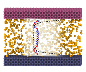
Here, we examine whether our kinetic model (2.17) can capture the non-equilibrium and dense gas effects of confined flows of the van der Waals fluids. The kinetic model is solved by the discrete velocity method together with the diffuse boundary condition, which is set at the position a half-molecule size away from the physical boundary as the molecule dimension is considered (see figure 1). The steady-state solutions are obtained using a semi-implicit iteration scheme (Su et al. Reference Su, Wang, Zhang and Wu2020), with the flow field initialised at the equilibrium state.

Figure 1. Schematic of (a) Poiseuille, (b) Couette, and (c) Couette–Fourier flows.
To validate the current kinetic model, MD simulations are conducted using a large-scale atomic/molecular massively parallel simulator (Thompson et al. Reference Thompson2022). In the MD simulations, fluid molecules interact with each other through the LJ potential (1.2), while the fluid–surface interaction is described by the diffuse boundary condition, to be consistent with the kinetic simulations. For initialisation, molecular velocities are generated with a Gaussian distribution to produce the required temperature, followed by a run of  $5\times 10^4$ steps in the constant number, volume, temperature ensemble to ensure that the initial states (mass, momentum and energy) are the same for the MD and kinetic simulations. Afterwards, the constant number, volume, energy ensemble is applied to fluid molecules to run all the cases with sufficient time steps and obtain the flow field data. The parameters for energy and size (molecule diameter) are obtained through the critical temperature and volume of the fluids (Chung et al. Reference Chung, Ajlan, Lee and Starling1988), respectively, as
 \begin{equation} \epsilon=\frac{k_BT_c}{1.2593},\quad \sigma =\left(\frac{MV_c}{N_A{\rm \pi}}\right)^{{1}/{3}}, \end{equation}
where  $T_c$ is the critical temperature (K), $\sigma$ is the molecular diameter (m), $V_c=1/\rho _c$ is the critical volume ( $\textrm {m}^3\ \textrm {kg}^{-1}$), $M$ is the molar mass ( $\textrm {kg}\ \textrm {mol}^{-1}$), and $N_A$ is the Avogadro constant. For argon, the critical temperature $T_c=150.69$ K and critical density $\rho _c=535.60\ \textrm {kg}\ \textrm {m}^{-3}$ are chosen in this study.
We consider the van der Waals fluids confined between two parallel plates located at  $y=0$ and $y=H$, as shown in figure 1. In Poiseuille flow, the plates are kept stationary and all the fluid molecules are subjected to an external force $\boldsymbol {F}_{ext}$ in the $x$ direction. In the Couette and Couette–Fourier flows, the top and bottom plates move with velocities $u_w$ and $-u_w$ in opposite directions, which drive fluid molecules to move. In the Poiseuille and Couette flows, the temperatures of the top and bottom plates are identical, while the temperature of the top plate $T_h$ is higher than that of the bottom plate $T_c$ in the Couette–Fourier flow.
3.1. Model analysis and comparison
The pair correlation function plays an essential role in the MET. A key requirement for determining the pair correlation function is that  $\chi \to 1$ as $n \to 0$, so that the Enskog-type equation for dense gases reduces to the Boltzmann-type equation in the dilute gas limit. However, the MET does not satisfy this requirement when the van der Waals pressure is chosen, as shown by (1.4), which makes the MET inaccurate in capturing the effect of the long-range molecular attraction. A temperature-dependent diameter (Hanley et al. Reference Hanley, McCarty and Cohen1972) can be employed to correct this error, which relates the co-volume $V_0$ with the second virial coefficient $B$ through $V_0 =B+T\,\mathrm {d}B/\mathrm {d}T$, and leads directly to the following EoS for real gases:
 \begin{equation} p=Znk_BT, \quad Z=1+n\chi\left(B+T\,\frac{\mathrm{d}B}{\mathrm{d}T}\right), \end{equation}
where  $Z$ is the compressibility factor. Clearly, the real gas EoS recovers the ideal gas EoS as the compressibility factor $Z \to 1$ when $n \to 0$. However, the compressibility factor $Z$ may be less than unity near the critical temperature (Mahmoud Reference Mahmoud2014), which means that the pair correlation function $\chi$ may be negative in (3.2a,b) as both $n>0$ and $V_0 =B+T\,\mathrm {d}B/\mathrm {d}T>0$, thus leading to negative shear viscosity and thermal conductivity, as can be seen from (2.8) and (2.9), which is physically inappropriate. Therefore, the MET is not suitable for modelling gas dynamics of the van der Waals fluids.
As shown in figure 2, the Enskog prediction overestimates the shear viscosity and thermal conductivity at large densities. The assumption of a state-dependent diameter (2.7) attenuates this overestimation at low temperatures (see figure 2a), but leads to an overestimation of the shear viscosity at low densities (see figure 2b). Overall, the correlated Enskog model agrees well with the experimental data for a wide range of temperatures and densities, particularly for shear viscosity and thermal conductivity, which indicates the importance of molecular attraction.

Figure 2. Comparison of transport coefficients of argon: (a,b) for the shear viscosity at  $T= 173.0$ K and 298.0 K, respectively, with the experimental data from Haynes (Reference Haynes1973); (c,d) for the thermal conductivity at $T= 298.15$ K and 348.15 K, respectively, with the experimental data from Michels, Sengers & Van de Klundert (Reference Michels, Sengers and Van de Klundert1963); and (e,f) for the bulk viscosity with the experimental data from Malbrunot et al. (Reference Malbrunot, Boyer, Charles and Abachi1983) and Madigosky (Reference Madigosky1967), respectively. The correlated Enskog model considers the effect of gas attraction on shear viscosity and thermal conductivity using the approach of Chung et al. (Reference Chung, Ajlan, Lee and Starling1988), and on the bulk viscosity using the approach of Hoover et al. (Reference Hoover, Ladd, Hickman and Holian1980b). The softened Enskog uses a state-dependent molecule diameter (2.7) in the Enskog prediction of transport coefficients (2.32). The Enskog (corrected $\mu _B$) uses the corrected bulk viscosity in the Enskog prediction of shear viscosity (2.33).
Similar to shear viscosity and thermal conductivity, molecular attraction is important for bulk viscosity. However, the bulk viscosity is predicted more accurately by the Enskog formula (2.32) with a state-dependent diameter (2.7), i.e. the softened Enskog prediction, as shown in figures 2(e) and 2(f). Consequently, the Enskog prediction of shear viscosity and thermal conductivity is in better agreement with the experimental data at large densities if we use this corrected bulk viscosity in (2.33), replacing the original hard-sphere bulk viscosity  $\mu _B^{hs}$ (see figures 2a,b,c,d). So the overestimation of bulk viscosity from the Enskog theory leads to the overestimation of shear viscosity and thermal conductivity (see figures 2a,b,c,d) at large densities.
To evaluate the effect of viscosity models on gas dynamics, a Poiseuille-type flow is investigated with the bottom and top wall temperatures  $T_c=173$ K and $T_h=373$ K, respectively, the averaged density $\rho _{avg}=150\ \textrm {kg}\ \textrm {m}^{-3}$, the channel width $H=15$ nm, and the external force $F_{ext}=0.0003\ \textrm {kcal}\ \textrm {mol}^{-1}\ \textrm {\AA }^{-1}$. The profiles of gas density, viscosity and velocity distributions are shown in figure 3. Although the density distribution is barely changed, the molecular attraction affects the velocity and viscosity profiles obviously.

The present kinetic model (2.17) will then be evaluated by comparison with the simulation results of MD, the Shakhov–Enskog model (Wang et al. Reference Wang, Wu, Ho, Li, Li and Zhang2020), and the NS equations. For incompressible, steady-state and laminar flows, the NS equations reduce to
 \begin{gather} \mu\,\frac{\partial^2 u}{\partial y^2}+F_{ext}n=0, \end{gather}
 \begin{gather}\kappa\,\frac{\partial^2~T}{\partial y^2}+\mu \left(\frac{\partial u}{\partial y}\right)^2=0, \end{gather}
with the second-order boundary condition for velocity slip and the first-order boundary condition for temperature jump, namely
 \begin{gather} u_s=\left.\pm A_1\lambda\,\frac{\partial u}{\partial y}\right|_{y=0}-\left.A_2\lambda^2\,\frac{\partial^2 u}{\partial y^2}\right|_{y=0}, \end{gather}
 \begin{gather}T_j=\left.\beta\,\frac{2\gamma}{\gamma+1}\,\frac{\lambda}{Pr}\,\frac{\partial T}{\partial y}\right|_{y=0}, \end{gather}
where the slip coefficients  $A_1=1.0$ and $A_2=0.5$ are chosen (Chapman & Cowling Reference Chapman and Cowling1990), and $\beta =(2-\sigma _T)/\sigma _T$ with the chosen thermal accommodation coefficient $\sigma _T=1.0$.
3.2. Poiseuille flows
In Poiseuille flows, an external body force acts on all the fluid molecules in the  $x$ direction with the wall temperature $T_w=273$ K. By solving (3.3) and (3.4), the velocity and temperature distribution across the channel can be obtained as
 \begin{gather} u(y)={-}\frac{F_{ext}n}{2\mu}\,[y^2-yH-H^2(A_1\,{Kn} +2A_2\,{Kn}^2)], \end{gather}
 \begin{gather}T(y)={-}\frac{(F_{ext}n)^2}{24\mu \kappa}\,(2y^4-4Hy^3+3H^2y^2-H^3y-L_TH^4)+T_w, \end{gather}
where  $Kn$ is the Knudsen number defined as
 \begin{equation} {Kn}=\frac{1}{\sqrt{2}\,n{\rm \pi} \sigma^2\chi H}, \end{equation}
and  $L_T$ is the thermal jump length expressed as
 \begin{equation} L_T=\beta\,\frac{2\gamma}{\gamma+1}\,\frac{{Kn}}{Pr}. \end{equation}
 Figure 4 shows the density and velocity profiles of the Poiseuille flows under a small external body force at different densities, i.e. different degrees of non-equilibrium (rarefaction) effect. As shown, the results of our kinetic model are in good agreement with the MD data for a broad range of densities (the reduced number density  $\eta$ ranges from 0.00031 to 0.14). By contrast, the Shakhov–Enskog model (Wang et al. Reference Wang, Wu, Ho, Li, Li and Zhang2020), which neglects the gas molecular attraction, overestimates the density near the wall and underestimates the overall velocity profiles, particularly at large densities. The reduced fluid density at the wall when the molecular attraction is considered is due to the ‘pull’ of the molecules in the bulk. The NS prediction, on the other hand, is better at large densities where the non-equilibrium effect is not significant.

Figure 4. Density and velocity profiles: (a,b) for  $\rho _{avg}=10\ \textrm {kg}\ \textrm {m}^{-3}$ ( $\eta = 0.00031$, $Kn = 2.56$); (c,d) for $\rho _{avg}=150\ \textrm {kg}\ \textrm {m}^{-3}$ ( $\eta = 0.047$, $Kn = 0.15$); and (e,f) for $\rho _{avg}=450\ \textrm {kg}\ \textrm {m}^{-3}$ ( $\eta = 0.14$, $Kn =0.039$). The external force $F_{ext} = 0.001\ \textrm {kcal}\ \textrm {mol}^{-1}\ \textrm {\AA }^{-1}$ is small, so the viscous dissipation is negligible, the channel width is $H=5$ nm, and the wall temperature is $T_w = 273$ K.
For high-speed flows, the viscous dissipation plays an important role, which is investigated in figure 5 with the average density  $\rho _{avg}=350\ \textrm {kg}\ \textrm {m}^{-3}$, channel width $H=5$ nm, and wall temperature $T_w=273$ K. Two large external forces are considered, namely $F_{ext}=0.01$ and $0.02\ \textrm {kcal}\ \textrm {mol}^{-1}\ \textrm {\AA }^{-1}$, respectively. Again, the density oscillation, parabolic velocity and quartic temperature profiles are well captured by the current kinetic model, while the Shakhov–Enskog model and the NS equation show large errors. The discrepancy in the results between the current kinetic model and the Shakhov–Enskog model suggests the important role of the long-range molecular attraction in gas dynamics, leading to reduced density near the wall, and enhanced velocity slip and temperature jump.

Figure 5. The density, velocity and temperature profiles at different external forces: (a–c) for  $F_{ext} = 0.01\ \textrm {kcal}\ \textrm {mol}^{-1}\ \textrm {\AA }^{-1}$; and (d–f) for $F_{ext} = 0.02\ \textrm {kcal}\ \textrm {mol}^{-1}\ \textrm {\AA }^{-1}$. The average density is $\rho _{avg}= 350\ \textrm {kg}\ \textrm {m}^{-3}$ ( $\eta =0.11$), the channel width is $H=5$ nm, and the wall temperature is $T_w= 273$ K. The resulting Knudsen number is $Kn=0.055$.
The effect of temperature on density and velocity profiles is shown in figure 6, with the average density  $\rho _{avg}=350\ \textrm {kg}\ \textrm {m}^{-3}$, channel width $H=5$ nm, and external force $F_{ext}=0.001\ \textrm {kcal}\ \textrm {mol}^{-1}\ \textrm {\AA }^{-1}$. It is very clear that the density and velocity profiles predicted by our kinetic model agree with the MD data, while the NS equation fails to predict density variation, and the Shakhov–Enskog model overpredicts the density near the wall. The main difference between our model and the Shakhov–Enskog model is that we include the gas molecular attraction, which can pull the gas molecules to the bulk. As a result, our prediction of the density at the wall is significantly smaller than the Shakhov–Enskog model for hard-sphere molecules, which ignores the molecular attraction. As shown in figure 6(e), even at high temperatures, the gas density of van der Waals fluids is still significantly affected by the long-range molecular attraction, i.e. the gas molecular attraction is not negligible even at high temperatures, which has largely been ignored in the previous studies.

Figure 6. The density and velocity profiles at different temperatures: (a,b) for  $T=253$ K; (c,d) for $T=313$ K; and (e,f) for $T=373$ K. The average density is $\rho _{avg}= 350\ \textrm {kg}\ \textrm {m}^{-3}$, the channel width is $H=5$ nm, and the external force is $F_{ext} = 0.001\ \textrm {kcal}\ \textrm {mol}^{-1}\ \textrm {\AA }^{-1}$.
The velocity decreases with the temperature, as shown in figures 6(b), 6(d) and 6(f), which is caused by the larger near-wall density and viscosity at high temperatures. The larger near-wall density means more efficient momentum transfer between the fluid and the wall, leading to smaller velocity slips at the solid surfaces, while the larger viscosity means more flow resistance for bulk fluid in the channel. This can be seen more clearly by normalising the slip velocity  $u_s$ by $F_{ext}H/(mu_m)$, namely
 \begin{equation} \hat{u}_s=\frac{u_smu_m}{F_{ext}H},\quad u_m=\sqrt{\frac{2k_BT}{m}}, \end{equation}
where  $u_m$ is the most probable velocity. The variation of the normalised slip velocity with temperature is shown in figure 7. The normalised slip velocity of hard-sphere gases predicted by the Shakhov–Enskog model is nearly constant as the temperature changes, while the present kinetic model and MD simulation predict a decreasing slip velocity with temperature. For the hard-sphere gases, the density distribution is not affected by the temperature and the velocity distribution $u(y)\propto 1/\mu _s^{hs}$. As shown by (2.8), the shear viscosity of hard-sphere gases satisfies $\mu _s^{hs} \propto \sqrt {T}$, so the normalised velocity is temperature-independent as $u_m \propto \sqrt {T}$. However, the relationship between viscosity and temperature $\mu _s \propto \sqrt {T}$ no longer holds for the van der Waals fluids as the collision integral $\varOmega ^{(2,2)}$, which is temperature-dependent, comes into play. Furthermore, a new dimensionless number, namely the reduced temperature $\hat {T}=k_BT/\epsilon$, is introduced to signify the competition between gas molecular attraction and kinetic energy for the van der Waals fluids. As the temperature increases, the gas molecules gain more kinetic energy to overcome the attractive forces holding them to the bulk. This results in greater accumulation of gas molecules near the walls, leading to the increased momentum transfer between the solid and the gas, thus reducing the slip velocity.

Figure 7. The variation of the normalised slip velocity with temperature.
As the viscous dissipation is non-negligible for fluids under high shear rates, we investigate its effect on the normalised mass flow rate  $Q_n$, which is defined as
 \begin{equation} Q_n= \frac{\displaystyle\int\nolimits_{0}^{H} n(y)\,u(y)\,\mathrm{d}y}{n_{avg}F_{ext}H^2/(mu_m)}. \end{equation}
As shown in figure 8, increased viscous dissipation reduces the mass flow rate in all the flow regimes. This is because the viscous dissipation leads to a smaller slip velocity and a larger flow resistance, as shown by the results in figure 5. The effect of viscous dissipation on mass flow rate is similar to that of confinement, which is also included in figure 8 for comparison. However, the confinement reduces the mass flow rate more significantly for small- ${Kn}$ flows, resulting in the disappearance of the Knudsen minimum. On the contrary, the viscous dissipation flattens the variation curve ( $Q_n \sim Kn$), but no Knudsen minimum disappearance is observed.

Figure 8. The variation of normalised mass flow rate with the Knudsen number at different external forces and confinements.
3.3. Couette flows
In the Couette flows, the top and bottom walls move at speed  $u_w$ in opposite directions, as shown in figure 1(b). No external force is exerted on fluid molecules, so $F_{ext}=0$ and the wall temperature is set to be $T_w=273$ K. The velocity and temperature profiles can also be obtained by solving (3.3) and (3.4), which are written as
 \begin{gather} u(y)=\frac{2u_w}{H}\,y-u_w, \end{gather}
 \begin{gather}T(y)={-}\frac{2\mu u_w^2}{\kappa H^2}\left(y^2-Hy-L_T H^2\right)+T_w. \end{gather}
 Figure 9 shows the density, velocity and temperature profiles of the Couette flows at different shear rates, with the average density  $\rho _{avg}=350\ \textrm {kg}\ \textrm {m}^{-3}$, and the channel width $H=5$ nm. The present kinetic model captures the density oscillation, linear velocity distribution and parabolic temperature distribution, which are in good agreement with the MD data. Similar to the Poiseuille flow, the Shakhov–Enskog model, which neglects the long-range attraction between gas molecules, overestimates the density near the wall, and underestimates both the velocity slip and the temperature jump. As the shear rate increases, gas molecules are more likely to accumulate near the wall, as the long-range molecular attraction may not be sufficient to pull the gas molecules to the bulk, also shown in figure 10. In contrast to the density peak near the wall, the viscosity is the lowest in this region; see figure 10(d). This is because the bulk gas has higher temperatures due to viscous heating. Figure 10(b) shows that stronger viscous dissipation causes a reduction in velocity slip as a combined consequence of a higher density peak and a greater viscosity near the wall.

Figure 9. The density, velocity and temperature profiles: (a–c)  $u_w=200\ \textrm {m}\ \textrm {s}^{-1}$; and (d–f) $u_w=400\ \textrm {m}\ \textrm {s}^{-1}$. The average density is $\rho _{avg}= 350\ \textrm {kg}\ \textrm {m}^{-3}$, the channel width is $H=5$ nm, and the wall temperature is $T_w= 273$ K.

Figure 10. Distribution of (a) density, (b) velocity, (c) temperature, and (d) viscosity across the channel at different wall velocities. The average density is  $\rho _{avg}= 350\ \textrm {kg}\ \textrm {m}^{-3}$, the channel width is $H=5$ nm, and the wall temperature is $T_w= 273$ K.
The viscous dissipation effect on Couette flows under tighter confinement is also investigated, where the channel width shrinks from 5 nm to 2 nm, as shown in figure 11. For such a case, both the non-equilibrium and confinement effects become stronger. The results from the Shakhov–Enskog model and the NS equations exhibit larger discrepancies compared to the MD simulation results, while our kinetic model can still capture accurately the density, velocity and temperature profiles.

Figure 11. The density, velocity and temperature profiles: (a–c)  $u_w=200\ \textrm {m}\ \textrm {s}^{-1}$; and (d–f) $u_w=400\ \textrm {m}\ \textrm {s}^{-1}$. The average density is $\rho _{avg} =350\ \textrm {kg}\ \textrm {m}^{-3}$, the channel width is $H=2$ nm, and the wall temperature is $T_w =273$ K. The resulting Knudsen number is $Kn=0.14$.
3.4. Couette–Fourier flows
The Couette–Fourier flow differs from the Couette flow only in the different wall temperatures, with the top wall temperature at  $T_h=373$ K and the bottom wall temperature at $T_c=273$ K. By solving (3.3) and (3.4), the velocity and temperature can be obtained as
 \begin{gather} u(y)=\frac{2u_w}{H}\,y-u_w, \end{gather}
 \begin{gather}\frac{T(y)-T_c}{T_h-T_c}={-}2\,{Br} \left[\left(\frac{y}{H}\right)^2-(1-2L_T)\,\frac{y}{H}-L_T(1-2L_T) \right]+\frac{y}{H}+L_T, \end{gather}
where  $Br =\mu u_w^2/[\kappa (T_h-T_c)]$ is the Brinkman number measuring the competition between viscous heating and thermal conduction.
The density, velocity and temperature profiles of the Couette–Fourier flows at two different wall velocities are shown in figure 12, with the channel width  $H=5$ nm. At a small wall moving velocity ( $u_w=50\ \textrm {m}\ \textrm {s}^{-1}$), the viscous dissipation is negligible, so the density and temperature distributions recover those of the Fourier flows, while the velocity distribution is similar to the Couette flows. When the wall velocity increases to $u_w=300\ \textrm {m}\ \textrm {s}^{-1}$, the temperature profile becomes a combination of the linear and parabola distributions resulting from the Fourier and Couette flows, respectively. Again, the present kinetic model predicts these profiles accurately, while the results of the Shakhov–Enskog model deviate significantly from the MD data, particularly for the density and temperature profiles.

Figure 12. The density, velocity and temperature profiles of the Couette–Fourier flows at different wall velocities: (a–c)  $u_w=50\ \textrm {m}\ \textrm {s}^{-1}$; and (d–f) $u_w=300\ \textrm {m}\ \textrm {s}^{-1}$. The average density is $\rho _{avg}=350\ \textrm {kg}\ \textrm {m}^{-3}$, the channel width is $H=5$ nm, and the top and bottom wall temperatures are $T_h=373$ K and $T_c=273$ K, respectively.
With increased viscous dissipation at large wall velocities, the heat generated in the gases leads to higher gas temperatures, as shown in figure 13(a). The viscous dissipation increases the heat transfer rate between the gas and the cold (bottom) wall, while it limits the heat transfer rate between the gas and the hot (top) wall, which can be seen clearly from the heat flux variation in figure 13(b). When the wall velocity is sufficiently large, the hot wall can also be heated by the gases due to the large amount of heat generated by viscous heating. Thus our kinetic model may provide a design simulation tool to develop next-generation technologies such as nanoscale evaporative cooling.

Figure 13. (a) Temperature and (b) heat flux distributions of the Couette–Fourier flows at different wall velocities, where the symbols denote the MD data. The averaged density is  $\rho _{avg}=350\ \textrm {kg}\ \textrm {m}^{-3}$, the channel width is $H=5$ nm, and the top and bottom wall temperatures are $T_h=373$ K and $T_c=273$ K, respectively.
3.5. Model solution in the dilute and continuum limits
As shown in figures 14(a) and 14(b), the results of the present kinetic model for the van der Waals fluids are in good agreement with the Shakhov–Boltzmann model for dilute gases and the MD simulation when the real gas effects (namely the volume exclusion and the long-range molecular attraction) and the confinement effect are negligible. This is because the density terms  $\mathcal {I}^{(1)}$ (2.15) and $\mathcal {I}^{(2)}$ (2.16) and the mean-field force (2.6) become negligible, and the kinetic model (2.17) reduces to the Shakhov model for the hard-sphere molecules in the dilute limit. Meanwhile, the results of our kinetic model, NS equations and MD simulations are very close in the continuum limit where the non-equilibrium and confinement effects are sufficiently small, as shown in figures 14(c) and 14(d). This is also expected because the NS equations are recovered from the kinetic model (2.17) in the small- ${Kn}$ limit, as shown in Appendix A. Therefore, the present kinetic model, which is an extension of the EV model for the hard-sphere molecules to consider real gas effects, is capable of simulating non-equilibrium flows of the confined van der Waals fluids.

Figure 14. The present kinetic model agrees with (a,b) the Boltzmann model in the dilute limit, and (c,d) the NS equations in the continuum limit. The average density  $\rho _{avg}= 2\ \textrm {kg}\ \textrm {m}^{-3}$, the channel width $H=100$ nm and the external force $F_{ext}=0.00003\ \textrm {kcal}\ \textrm {mol}^{-1}\ \textrm {\AA }^{-1}$ in (a,b) correspond to $\eta =0.00062$ and $Kn = 0.64$; the average density $\rho _{avg}= 450\ \textrm {kg}\ \textrm {m}^{-3}$, the channel width $H=50$ nm and the external force $F_{ext}=0.00005\ \textrm {kcal}\ \textrm {mol}^{-1}\ \textrm {\AA }^{-1}$ in (c,d) correspond to $\eta =0.14$ and $Kn = 0.0039$.
4. Conclusions
We have proposed a new kinetic model for confined flows of the van der Waals fluids that is consistent with the Boltzmann model in the dilute limit and with the NS equations in the continuum limit. The long-range molecular attraction is considered in both the kinetic equation and the transport coefficients (shear viscosity and thermal conductivity). Building upon the Enskog theory for dense gases, the kinetic model is capable of handling dilute to moderately dense gas flows at any Knudsen number. Through the Chapman–Enskog expansion, macroscopic equations can be obtained with a correct form of EoS if the pair correlation function is chosen appropriately, demonstrating the thermodynamic consistency of our kinetic model.
Further analysis shows that the shear viscosity and thermal conductivity are in better agreement with the experimental data when the molecular attraction is taken into account, while the bulk viscosity is more accurately predicted by the Enskog formula for the hard-sphere molecules with a state-dependent diameter. The Enskog theory greatly overestimates the bulk viscosity of dense gases, which explains the overestimation of shear viscosity and thermal conductivity at large densities. The empirical MET that incorporates the molecular attraction into the pair correlation function either fails to recover the Boltzmann equation in the dilute limit or produces non-physical properties, e.g. negative transport coefficients near critical temperatures. Momentum and energy transfer become temperature-dependent for the van der Waals fluids due to gas molecular attraction, which is not the case for the hard-sphere molecules. The extensive numerical tests suggest that the present model can capture the effects of non-equilibrium, confinement and real gas simultaneously. While this study is concerned primarily with the confined flows of van der Waals fluids, the present kinetic model can be applied to other types of flows, including unconfined flows and non-equilibrium evaporating flows. In this work, only monatomic gases are considered. Nevertheless, the developed model, with the transport coefficients corrected by the acentric factor, may be applicable to the polyatomic gases if the internal energies of molecules (i.e. rotational, vibrational and electronic energies) are thermalised rapidly with the translational energy. Otherwise, more terms should be added to account for the relaxation between the translational and internal modes during molecular collisions.
Acknowledgements
Supercomputer time on ARCHER is provided by the UK Consortium on Mesoscale Engineering Sciences (UKCOMES) under the UK Engineering and Physical Sciences Research Council grant no. EP/R029598/1. This work made use of computational support by CoSeC, the Computational Science Centre for Research Communities, through UKCOMES.
Funding
This work is supported by the UK's Engineering and Physical Sciences Research Council (grant no. EP/R041938/1).
Declaration of interests
The authors declare no competing interests.
Appendix A. Chapman–Enskog expansion of the present kinetic model
To properly assign the relaxation time  $\tau$ and the Prandtl number $Pr$, we will derive the hydrodynamic equations from the kinetic model (2.17) using the Chapman–Enskog expansion (Chapman & Cowling Reference Chapman and Cowling1990). First, the following expansions are introduced:
 \begin{equation} \frac{\partial}{\partial t}=\varepsilon\,\frac{\partial}{\partial t_1}+\varepsilon^{2}\,\frac{\partial}{\partial t_2},\quad \frac{\partial}{\partial \boldsymbol{r}}=\varepsilon\,\frac{\partial}{\partial \boldsymbol{r}_1}, \end{equation}
where  $\varepsilon$ is a small parameter on the order of the Knudsen number, and $t_1$ and $t_2$ are the fast convective and slow diffusive scales, respectively. The distribution function $f$, kinetic pressure tensor $\boldsymbol{\mathsf{P}}_k$, and kinetic heat flux $\boldsymbol {Q}_k$ satisfy
 \begin{equation} \mathcal{W}=\mathcal{W}^{(0)}+\varepsilon \mathcal{W}^{(1)}+\varepsilon^{2}\mathcal{W}^{(2)}+\cdots, \end{equation}
where  $\mathcal {W}=\{\,f, \boldsymbol{\mathsf{P}}_k, \boldsymbol {Q}_k\}$. Meanwhile, we also assume $\boldsymbol {F} = \varepsilon \boldsymbol {F}_0$, with $\boldsymbol {F} =\boldsymbol {F}_{ext} + \boldsymbol {F}_{att}$ being the total force term. Following (A1a,b) and (A2), the kinetic equation (2.17) can be transformed into a hierarchy of equations according to the order of $\varepsilon$, with the preceding equations given as
 \begin{equation} \left.\begin{aligned} \varepsilon^{0}: & \quad f^{(0)}=f^{eq},\\ \varepsilon^{1}: & \quad \frac{\partial f^{(0)}}{\partial t_1} + \boldsymbol{\xi} \boldsymbol{\cdot} \frac{\partial f^{(0)}}{\partial \boldsymbol{r}_1} + \frac{\boldsymbol{F}_{0}}{m} \boldsymbol{\cdot} \frac{\partial f^{(0)}}{\partial \boldsymbol{\xi}_1} \\ & \qquad \quad={-}\frac{1}{\tau}\left[f^{(1)}-f^{eq}(1-Pr)\,\frac{\boldsymbol{c}\boldsymbol{\cdot}\boldsymbol{Q}_k^{(1)}}{ 5p_0RT}\left(\frac{c^2}{RT}-5\right)\right]+\mathcal{I}^{(1)},\\ \varepsilon^{2}: & \quad \frac{\partial f^{(1)}}{\partial t_1} + \frac{\partial f^{(0)}}{\partial t_2} + \boldsymbol{\xi} \boldsymbol{\cdot} \frac{\partial f^{(1)}}{\partial \boldsymbol{r}_1} + \frac{\boldsymbol{F}_{0}}{m} \boldsymbol{\cdot} \frac{\partial f^{(1)}}{\partial \boldsymbol{\xi}_1} \\ & \qquad \quad={-}\frac{1}{\tau}\left[f^{(2)}-f^{eq}(1-Pr)\,\frac{\boldsymbol{c}\boldsymbol{\cdot}\boldsymbol{Q}_k^{(2)}} {5p_0RT}\left(\frac{c^2}{RT}-5\right)\right]+\mathcal{I}^{(2)}. \end{aligned}\right\} \end{equation}
Here,  $\mathcal {I}^{(1)}$ and $\mathcal {I}^{(2)}$ are of the order of $\varepsilon$ and $\varepsilon ^2$, respectively, as they include the first- and second-order gradients of macroscopic properties (density, velocity and temperature). From the result of the order $\varepsilon ^{0}$, we can get that
 \begin{equation} \int \varPsi_i\,f^{(k)}\,\mathrm{d}\boldsymbol{\xi}=0, \quad k\geqslant1, \end{equation}
where  $\varPsi _i=\{1, m\boldsymbol {\xi }, m\boldsymbol {\xi }^2/2\}$ are the summation invariants. Consequently, the hydrodynamic equations of the order of $\varepsilon ^{1}$ can be obtained as
 \begin{gather} \frac{\partial \rho}{\partial t_1}+\frac{\partial}{\partial \boldsymbol{r}_1}\boldsymbol{\cdot} (\rho \boldsymbol{u})=0, \end{gather}
 \begin{gather}\frac{\partial (\rho \boldsymbol{u})}{\partial t_1}+\frac{\partial}{\partial \boldsymbol{r}_1}\boldsymbol{\cdot} [\boldsymbol{\mathsf{P}}_k^{(0)} +\rho \boldsymbol{uu}]-n\boldsymbol{F}_0={-} \boldsymbol{\nabla}\boldsymbol{\cdot}[(nV_0\chi nk_BT)\boldsymbol{\mathsf{U}}], \end{gather}
 \begin{gather}\frac{\partial (\rho E)}{\partial t_1}+\frac{\partial}{\partial \boldsymbol{r}_1}\boldsymbol{\cdot} [\boldsymbol{Q}_k^{(0)}+\rho E \boldsymbol{u}+ \boldsymbol{\mathsf{P}}_k^{(0)} \boldsymbol{\cdot}\boldsymbol{u}]-n\boldsymbol{F}_0\boldsymbol{\cdot} \boldsymbol{u}={-}\boldsymbol{\nabla}\boldsymbol{\cdot} (nV_0\chi nk_BT \boldsymbol{u}), \end{gather}
where  $\boldsymbol{\mathsf{U}}$ is the unit tensor, and $E=(3RT+\boldsymbol {u}^2)/2$ is the combination of internal and kinetic energies of molecules per unit mass. It is noted that the potential energy of molecules is described by the excess collision terms $\mathcal {I}^{(1)}$ and $\mathcal {I}^{(2)}$ as well as the mean-field force term $\boldsymbol {F}_{att}$ in the kinetic model, so it does not appear in $E$. The terms on the right-hand side of (A5b) and (A5c) quantify the effect of the non-local collisions of gas molecules, which are negligible for dilute gases. The zeroth-order pressure tensor $\boldsymbol{\mathsf{P}}_k^{(0)}$ and heat flux $\boldsymbol {Q}_k^{(0)}$ can be calculated as
 \begin{equation} \left.\begin{gathered} \boldsymbol{\mathsf{P}}_k^{(0)}=\int m\boldsymbol{cc}\,f^{(0)}\,\mathrm{d}\boldsymbol{\xi} = nk_BT\boldsymbol{\mathsf{U}}, \\ \boldsymbol{Q}_k^{(0)} = \int \frac{mc^2\boldsymbol c}{2}\,f^{(0)}\,\mathrm{d}\boldsymbol{\xi}=0. \end{gathered}\right\} \end{equation}
 Similarly, the hydrodynamic equations of the order of  $\varepsilon ^{2}$ can be obtained by taking the moments in terms of the summation invariants $\varPsi _i$ as
 \begin{equation} \left.\begin{gathered} \frac{\partial \rho}{\partial t_2}=0,\\ \frac{\partial (\rho \boldsymbol{u})}{\partial t_2}+\frac{\partial}{\partial \boldsymbol{r}_1} \boldsymbol{\cdot} \boldsymbol{\mathsf{P}}_k^{(1)} =\boldsymbol{\nabla}\boldsymbol{\cdot} [\mu_B(\boldsymbol{\nabla}\boldsymbol{\cdot}\boldsymbol{u})\boldsymbol{\mathsf{U}}],\\ \frac{\partial (\rho E)}{\partial t_2}+\frac{\partial}{\partial \boldsymbol{r}_1}\boldsymbol{\cdot} [\boldsymbol{Q}_k^{(1)}+ \boldsymbol{\mathsf{P}}_k^{(1)} \boldsymbol{\cdot}\boldsymbol{u}] =\boldsymbol{\nabla}\boldsymbol{\cdot} [\mu_B(\boldsymbol{\nabla}\boldsymbol{\cdot}\boldsymbol{u})\boldsymbol{u}]. \end{gathered}\right\} \end{equation}
 From the result of the order  $\varepsilon ^1$ in (A3), $f^{(1)}$ can be obtained as
 \begin{equation} f^{(1)}={-}\tau \left[\frac{\partial f^{(0)}}{\partial t_1} + \boldsymbol{\xi} \boldsymbol{\cdot} \frac{\partial f^{(0)}}{\partial \boldsymbol{r}_1} + \frac{\boldsymbol{F}_0}{m} \boldsymbol{\cdot} \frac{\partial f^{(0)}}{\partial \boldsymbol{\xi}_1}\right] +f^{eq}(1-Pr)\,\frac{\boldsymbol{c}\boldsymbol{\cdot}\boldsymbol{Q}_k^{(1)}}{5p_0RT} \left(\frac{c^2}{RT}-5\right)+\tau \mathcal{I}^{(1)}. \end{equation}
Therefore, the first-order pressure tensor  $\boldsymbol{\mathsf{P}}_k^{(1)}$ and heat flux $\boldsymbol {Q}_k^{(1)}$ can be calculated as
 \begin{equation} \left.\begin{gathered} \boldsymbol{\mathsf{P}}_k^{(1)}=\int m\boldsymbol{cc}\,f^{(1)}\,\mathrm{d}\boldsymbol{\xi}={-}2nk_BT\tau\left(1+ \frac{2}{5}\,nV_0\chi\right) \mathring{\boldsymbol{\mathsf{S}}} , \\ \boldsymbol{Q}_k^{(1)} =\int \frac{mc^2\boldsymbol{c}}{2}\,f^{(1)}\,\mathrm{d}\boldsymbol{\xi}={-} \frac{5k_B}{2m}\,\frac{nk_BT\tau}{Pr}\left(1+\frac{3}{5}\,nV_0\chi\right) \boldsymbol{\nabla} T, \end{gathered}\right\} \end{equation}
where the rate-of-shear tensor  $\mathring {\boldsymbol{\mathsf{S}}}$ can be expressed as
 \begin{equation} \mathring{\boldsymbol{\mathsf{S}}}=\tfrac{1}{2}\left[\boldsymbol{\nabla}\boldsymbol{u}+( \boldsymbol{\nabla}\boldsymbol{u})^{\rm T}\right]-\tfrac{1}{3}(\boldsymbol{\nabla}\boldsymbol{\cdot} \boldsymbol{u})\boldsymbol{\mathsf{U}}, \end{equation}
where  $(\boldsymbol {\nabla }\boldsymbol {u})^\textrm {T}$ denotes the transpose of $\boldsymbol {\nabla }\boldsymbol {u}$.
If the molecular size is not negligible, then the momentum and energy can be transferred at the instant collisions over a molecule size  $\sigma$. According to Cercignani & Lampis (Reference Cercignani and Lampis1988) and Frezzotti (Reference Frezzotti1999), the collisional pressure tensor $\boldsymbol{\mathsf{P}}_c$ and heat flux $\boldsymbol {Q}_c$ relate to the collision operator through
 \begin{equation} \left.\begin{gathered} \int m\boldsymbol{\xi} [J_s^{(0)}+\mathcal{I}^{(1)}+\mathcal{I}^{(2)}]\,\mathrm{d}\boldsymbol{\xi}={-} \boldsymbol{\nabla}\boldsymbol{\cdot}\boldsymbol{\mathsf{P}}_c, \\ \int \frac{m\xi^2}{2}\,[J_s^{(0)}+\mathcal{I}^{(1)}+\mathcal{I}^{(2)}]\,\mathrm{d}\boldsymbol{\xi}={-} \boldsymbol{\nabla}\boldsymbol{\cdot}(\boldsymbol{Q}_c+\boldsymbol{\mathsf{P}}_c\boldsymbol{\cdot}\boldsymbol{u}), \end{gathered}\right\} \end{equation}
from which we can get
 \begin{equation} \left.\begin{gathered} \boldsymbol{\mathsf{P}}_c=[nk_BTnV_0\chi -\mu_B(\boldsymbol{\nabla}\boldsymbol{\cdot}\boldsymbol{u})]\boldsymbol{\mathsf{U}}, \\ \boldsymbol{Q}_c=0. \end{gathered}\right\} \end{equation}
Combining (A5) and (A7), the hydrodynamic equations can be obtained as
 \begin{gather} \frac{\partial \rho}{\partial t}+\boldsymbol{\nabla}\boldsymbol{\cdot}(\rho \boldsymbol{u})=0, \end{gather}
 \begin{gather}\frac{\partial (\rho \boldsymbol{u})}{\partial t}+\boldsymbol{\nabla}\boldsymbol{\cdot}(\rho \boldsymbol{uu}+\boldsymbol{\mathsf{P}}_k+\boldsymbol{\mathsf{P}}_c)-n(\boldsymbol{F}_{att}+\boldsymbol{F}_{ext})=0, \end{gather}
 \begin{gather}\frac{\partial (\rho E)}{\partial t}+\boldsymbol{\nabla}\boldsymbol{\cdot}[\rho E \boldsymbol{u}+\boldsymbol{Q}_k+ (\boldsymbol{\mathsf{P}}_k+\boldsymbol{\mathsf{P}}_c)\boldsymbol{\cdot}\boldsymbol{u}]-n(\boldsymbol{F}_{att}+ \boldsymbol{F}_{ext})\boldsymbol{\cdot}\boldsymbol{u}=0, \end{gather}
where  $\boldsymbol{\mathsf{P}}_k=\boldsymbol{\mathsf{P}}_k^{(0)}+\boldsymbol{\mathsf{P}}_k^{(1)}$ and $\boldsymbol {Q}_k=\boldsymbol {Q}_k^{(0)}+\boldsymbol {Q}_k^{(1)}$ are the kinetic parts of the pressure tensor and heat flux, respectively. Now we make further analysis on the mean-field force term $\boldsymbol {F}_{att}$. When the long-range attractive forces between gas molecules are considered, the intermolecular potential energy comes into play (Chapman & Cowling Reference Chapman and Cowling1990; Martys Reference Martys1999; He & Doolen Reference He and Doolen2002). Assuming that the spatial variation of density is small in the hydrodynamic limit, the mean-field force $\boldsymbol {F}_{att}$ can be approximated by
 \begin{equation} \boldsymbol{F}_{att} = 2a\,\boldsymbol{\nabla} n+k\,\boldsymbol{\nabla}\nabla^2n, \end{equation}
where  $a$ and $k$ are two constants related to the attractive potential as
 \begin{equation} \left.\begin{gathered} a={-}\tfrac{1}{2}\int_{r>\sigma}\phi_{att}(r)\,\mathrm{d}\boldsymbol{r}, \\ k={-}\tfrac{1}{6}\int_{r>\sigma}r^2\,\phi_{att}(r)\,\mathrm{d}\boldsymbol{r}. \end{gathered}\right\} \end{equation}
Considering the identity  $n\,\boldsymbol {\nabla }\nabla ^2n$ in the form
 \begin{equation} n\,\boldsymbol{\nabla}\nabla^2 n=\boldsymbol{\nabla}\boldsymbol{\cdot} \left[\left(n\,\nabla^2n+\tfrac{1}{2}|\boldsymbol{\nabla}n|^2\right)\boldsymbol{\mathsf{U}}-\boldsymbol{\nabla}n\, \boldsymbol{\nabla} n\right], \end{equation}
the mean-field force term in (A5) can be transformed as
 \begin{equation} n\boldsymbol{F}_{att}=\boldsymbol{\nabla}\boldsymbol{\cdot}\boldsymbol{\mathsf{P}}_{att} +\boldsymbol{\nabla} \boldsymbol{\cdot}\boldsymbol{\mathsf{K}}, \end{equation}
where  $\boldsymbol{\mathsf{P}}_{att}=an^2\boldsymbol{\mathsf{U}}$ is the pressure contribution due to attractive forces, and $\boldsymbol{\mathsf{K}}$ is the capillary (or Korteweg stress) tensor (Anderson, McFadden & Wheeler Reference Anderson, McFadden and Wheeler1998), which is given by
 \begin{equation} \boldsymbol{\mathsf{K}}=k\left[\left(n\nabla^2n+\tfrac{1}{2}|\boldsymbol{\nabla}n|^2\right)\boldsymbol{\mathsf{U}}-\boldsymbol{\nabla} n\,\boldsymbol{\nabla}n\right]. \end{equation}
 The total pressure tensor  $\boldsymbol{\mathsf{P}}$ and heat flux $\boldsymbol {Q}$ are the combination of kinetic and potential contributions, which are
 \begin{equation} \left.\begin{aligned} \boldsymbol{\mathsf{P}} & =\boldsymbol{\mathsf{P}}_k+\boldsymbol{\mathsf{P}}_c+\boldsymbol{\mathsf{P}}_{att}\\ & =[nk_BT(1+nV_0\chi)-an^2 -\mu_B(\boldsymbol{\nabla}\boldsymbol{\cdot} \boldsymbol{u})]\boldsymbol{\mathsf{U}}-2nk_BT\tau\left(1+\frac{2}{5}\,nV_0\chi\right) \mathring{\boldsymbol{\mathsf{S}}}, \\ \boldsymbol{Q} & =\boldsymbol{Q}_k+\boldsymbol{Q}_c={-}\frac{5k_B}{2m}\,\frac{nk_BT\tau}{Pr}\left(1+\frac{3}{5}\,nV_0\chi\right) \boldsymbol{\nabla} T. \end{aligned}\right\} \end{equation}
Comparing (A19) to Newton's law of viscosity and Fourier's law of thermal conduction, the relationship between the relaxation time and transport coefficients can be obtained as
 \begin{equation} \left.\begin{gathered} \mu_s=nk_BT\tau\left(1+\frac{2}{5}\,nV_0\chi\right), \\ \kappa=\frac{5k_B}{2m}\,\frac{nk_BT\tau}{Pr}\left(1+\frac{3}{5}\,nV_0\chi\right). \end{gathered}\right\} \end{equation}
Finally, combining (A13) and (A17), we obtain the hydrodynamic equations of the kinetic model (2.17) in the conservative form as
 \begin{equation} \left.\begin{gathered} \frac{\partial \rho}{\partial t}+\boldsymbol{\nabla}\boldsymbol{\cdot}(\rho \boldsymbol{u})=0,\\ \frac{\partial (\rho \boldsymbol{u})}{\partial t}+\boldsymbol{\nabla} \boldsymbol{\cdot}\{\rho \boldsymbol{uu}+[p-\mu_B(\boldsymbol{\nabla}\boldsymbol{\cdot} \boldsymbol{u})]\boldsymbol{\mathsf{U}}-2\mu_s\mathring{\boldsymbol{\mathsf{S}}}-\boldsymbol{\mathsf{K}}\}=n\boldsymbol{F}_{ext},\\ \frac{\partial (\rho E)}{\partial t}+\boldsymbol{\nabla}\boldsymbol{\cdot}\{\rho E \boldsymbol{u}-\kappa \boldsymbol{\nabla}T+ [p-\mu_B(\boldsymbol{\nabla}\boldsymbol{\cdot}\boldsymbol{u})] \boldsymbol{\mathsf{U}}\boldsymbol{\cdot}\boldsymbol{u} -(2\mu_s\mathring{\boldsymbol{\mathsf{S}}}+\boldsymbol{\mathsf{K}}) \boldsymbol{\cdot}\boldsymbol{u}\} =n\boldsymbol{F}_{ext}\boldsymbol{\cdot}\boldsymbol{u}, \end{gathered}\right\} \end{equation}
where the pressure  $p$ in both the momentum and energy equations satisfies
 \begin{equation} p=nk_BT(1+nV_0\chi)-an^2. \end{equation}
Noted that if there is no interface, e.g. for single phase flows, then the capillary force does not appear, and the hydrodynamic equations (A21) reduce to the conventional NS equations for compressible flows.


