


1. Introduction
The displacement of an interface between two Newtonian fluids driven through a narrow gap bounded by elastic walls is a fundamental two-phase fluid–structure interaction that occurs in many industrial, geophysical and biological processes (Juel, Pihler-Puzović & Heil Reference Juel, Pihler-Puzović and Heil2018). In the absence of fluid inertia, the behaviour of the interface is determined by the interplay between the interfacial surface tension; the viscosities of the fluids; and the elastic properties of the wall. Although the inertialess equations governing the bulk response of the fluids, the Stokes equations, are linear, nonlinearities arise due to the presence of (i) the interface and (ii) the elastic walls.
Elastic walls are not required to elicit complex behaviour; indeed, the Saffman–Taylor viscous fingering instability in a rigid Hele-Shaw channel, a channel whose width is much greater than its height (Saffman & Taylor Reference Saffman and Taylor1958), is an exemplar of non-trivial interfacial dynamics. Precisely because of its fundamental nature and the implications for transport of multi-phase flows and flow in porous media, viscous fingering has been extensively studied, see Homsy (Reference Homsy1987), Couder (Reference Couder2000) and Casademunt (Reference Casademunt2004) for reviews. Moreover, the introduction of non-Newtonian effects (Lindner et al. Reference Lindner, Bonn, Poiré, Ben Amar and Meunier2002) or fluid inertia (Chevalier et al. Reference Chevalier, Ben Amar, Bonn and Lindner2006) does not fundamentally change the fingering and can be accommodated by suitable redefinitions of the control parameter.
More recently, attention has turned to control or suppression of the fingering by varying the flow rate (Li et al. Reference Li, Lowengrub, Fontana and Palffy-Muhoray2009; Dias, Parisio & Miranda Reference Dias, Parisio and Miranda2010; Dias et al. Reference Dias, Alvarez-Lacalle, Carvalho and Miranda2012); adjusting the viscosity ratio of the two fluids (Bischofberger, Ramachandran & Nagel Reference Bischofberger, Ramachandran and Nagel2014); introducing particles (Luo, Chen & Lee Reference Luo, Chen and Lee2018); and modifying the channel geometry either statically (Al-Housseiny, Tsai & Stone Reference Al-Housseiny, Tsai and Stone2012; Dias & Miranda Reference Dias and Miranda2013; Jackson et al. Reference Jackson, Power, Giddings and Stevens2017; Bongrand & Tsai Reference Bongrand and Tsai2018) or dynamically via the introduction of elastic walls (Pihler-Puzović et al. Reference Pihler-Puzović, Illien, Heil and Juel2012; Al-Housseiny, Christov & Stone Reference Al-Housseiny, Christov and Stone2013; Lister, Peng & Neufeld Reference Lister, Peng and Neufeld2013) or via a time-varying displacement of rigid walls (Zheng, Kim & Stone Reference Zheng, Kim and Stone2015; Morrow, Moroney & McCue Reference Morrow, Moroney and McCue2019; Vaquero-Stainer et al. Reference Vaquero-Stainer, Heil, Juel and Pihler-Puzović2019). The majority of these studies have been conducted in radial geometries in which the average interfacial propagation speed decreases with distance from the injection point for a constant injected volume flux. In such geometries, a steadily propagating state is never possible.
In this paper, we replace the upper wall of an otherwise rigid Hele-Shaw channel by an elastic sheet, see figure 1, to make an elasto-rigid channel. If fluid is injected from one end of the channel then it is possible for a steadily propagating state to develop. The propagation of an air finger into a collapsed elasto-rigid channel is a simplified model for pulmonary airway reopening (Gaver et al. Reference Gaver, Halpern, Jensen and Grotberg1996; Hazel & Heil Reference Hazel and Heil2003; Heap & Juel Reference Heap and Juel2009; Ducloué et al. Reference Ducloué, Hazel, Thompson and Juel2017b), but our focus in this paper is primarily on the nonlinear behaviour of the depth-averaged, elasto-rigid system rather than on any applications to pulmonary mechanics.

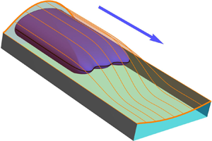
Figure 1. The elasto-rigid channel consists of two rigid sidewalls, a rigid lower wall and a deformable upper wall. The cross-section of the channel has width  $W^{*}$ and undeformed height $b^{*}_{0}$. The height of the deformed sheet is $b^{*}(x^{*}_{1},x^{*}_{2})$. An air finger propagates into the fluid-filled channel along the $x^{*}_{1}$ direction.
Our study directly complements the experimental investigations of Ducloué et al. (Reference Ducloué, Hazel, Pihler-Puzović and Juel2017a,Reference Ducloué, Hazel, Thompson and Juelb) who observed several different modes of interface propagation in elasto-rigid channels. Ducloué et al. (Reference Ducloué, Hazel, Thompson and Juel2017b) found that, for constant interfacial propagation speed, the complexity of the propagation modes increases with increasing levels of initial collapse of the channel. For modest initial collapse, a single air finger reopens the channel as it propagates steadily and adopts a shape that is reminiscent of a single Saffman–Taylor finger in a rigid channel. At higher levels of collapse the elastic channel reopens over a shorter axial length scale, for a fixed interfacial propagation speed, and, consequently, the interface propagates into a converging gap. In this geometric configuration, the interface is unstable and the instability leads to the formation of small-scale unsteady fingers. Ducloué et al. (Reference Ducloué, Hazel, Pihler-Puzović and Juel2017a) conjectured that the small-scale fingers are analogous to those that develop during peeling of an adhesive strip (McEwan & Taylor Reference McEwan and Taylor1966) and those seen in the printer's instability on an interface between two rotating rigid cylinders (Couder Reference Couder2000). Cuttle, Pihler-Puzović & Juel (Reference Cuttle, Pihler-Puzović and Juel2020) investigated the behaviour of a strongly collapsed elasto-rigid channel experimentally and found a number of different finger morphologies whose geometric complexity increased with increasing propagation speed from simple Saffman–Taylor-like fingers to highly disordered interfaces with multiple tips that evolve continually in time. Cuttle et al. (Reference Cuttle, Pihler-Puzović and Juel2020) also identified regions of non-trivial transient dynamics that suggested the existence of unstable states mediating the transition between different steadily propagating states.
In contrast to the elasto-rigid system, the experimentally observed two-phase flow in an equivalent rigid geometry over the same parameter range is relatively simple. If a more viscous fluid (oil) is displaced by a less viscous one (air) injected from one end of a rigid Hele-Shaw channel, an initially flat interface can exhibit multiple tips transiently, but ultimately a single symmetric finger emerges and propagates at constant speed (Saffman & Taylor Reference Saffman and Taylor1958). In this geometry, the height of the channel's cross-section is much smaller than its width and consequently the flow within the channel can be effectively described using a depth-averaged theory. The simplest two-phase, depth-averaged model does not include surface tension because the perturbation to the interface curvature does not feature at leading order in the expansion in inverse cross-sectional aspect ratio. In the absence of surface tension, however, the model has continuous families of symmetric and asymmetric (Taylor & Saffman Reference Taylor and Saffman1959) solutions at the same flow rate. McLean & Saffman (Reference McLean and Saffman1981) showed that the ad hoc introduction of surface tension qualitatively reproduces the experimental observations by selecting a single finger from the symmetric solution family at each flow rate. Additional unstable symmetric solutions of the McLean & Saffman (Reference McLean and Saffman1981) model were later found by Romero (Reference Romero1982) and Vanden-Broeck (Reference Vanden-Broeck1983) and shown to correspond to symmetric fingers with multiple tips by Gardiner et al. (Reference Gardiner, McCue, Lustri and Moroney2015). Park & Homsy (Reference Park and Homsy1984) showed that quantitative agreement with experiments requires the inclusion of corrections due to the presence of liquid films that remain on the channel walls after propagation of the air finger. The necessity of including these liquid-film corrections was later confirmed by the detailed experiments of Tabeling & Libchaber (Reference Tabeling and Libchaber1986).
Although the depth-averaged model system describing two-phase flow in a rigid Hele-Shaw channel has multiple possible solutions only the symmetric, single-tipped finger is stable (Bensimon, Pelce & Shraiman Reference Bensimon, Pelce and Shraiman1987; Tanveer Reference Tanveer1987). Experimental observations have shown, however, that the finger becomes unstable to tip splitting (Tabeling, Zocchi & Libchaber Reference Tabeling, Zocchi and Libchaber1987) and fluctuations in width (Moore et al. Reference Moore, Juel, Burgess, McCormick and Swinney2003) at high driving flow rates in channels of sufficiently large cross-sectional aspect ratio. Tabeling et al. (Reference Tabeling, Zocchi and Libchaber1987) showed that the flow rate at which instabilities first occur is strongly dependent on channel roughness and Couder (Reference Couder2000) suggested that the tip-splitting instability is a noise-induced subcritical transition to nearby alternative states.
Rather than relying on uncontrolled perturbations to provoke instability, further studies introduced well-defined perturbations into either the depth-averaged model system or the geometry of the Hele-Shaw channel; see the review by Couder (Reference Couder2000). These perturbed systems exhibit symmetry breaking and tip splitting, as well as periodic and complex time-dependent behaviour. More recently, Thompson, Juel & Hazel (Reference Thompson, Juel and Hazel2014) introduced a prescribed depth perturbation (a longitudinal ridge) into the model of McLean & Saffman (Reference McLean and Saffman1981) and showed that this leads to interaction between solutions of the unperturbed system. For example, the symmetric finger exchanges stability with an asymmetric finger at a critical flow rate via a symmetry-breaking bifurcation. The solution structure and sequence of symmetry-breaking and Hopf bifurcations agreed qualitatively with previous experimental observations in channels with cross-sections designed to mimic collapsed elastic tubes (de Lózar et al. Reference de Lózar, Heap, Box, Hazel and Juel2009; Pailha et al. Reference Pailha, Hazel, Glendinning and Juel2012). Quantitative agreement between the depth-averaged model and experimental measurements of finger widths for the multiple solutions was subsequently obtained for these depth-perturbed channels with sufficiently large cross-sectional aspect ratios (Franco-Gómez et al. Reference Franco-Gómez, Thompson, Hazel and Juel2016). Thus, in perturbed rigid channels the multiple solutions of the depth-averaged model can be directly related to the complex behaviour observed in experiments.
Having established that depth-averaged models can be used to describe the observed two-phase flow phenomena in perturbed rigid Hele-Shaw channels, our aims in the present study are twofold: (i) to develop an accurate, depth-averaged model for the elasto-rigid system; and (ii) to use the model to examine the connection between the multiple modes of finger propagation observed by Ducloué et al. (Reference Ducloué, Hazel, Thompson and Juel2017b) and the known multiple solutions in depth-averaged models of two-phase flow in perturbed rigid Hele-Shaw channels (Franco-Gómez et al. Reference Franco-Gómez, Thompson, Hazel and Juel2016).
The rest of this paper is divided into three parts. In § 2, we describe the depth-averaged model used to describe the propagating finger and the reopening of the channel as well as its numerical solution using finite element methods. In § 3 we demonstrate the good quantitative agreement between the model and the experimental data of Ducloué et al. (Reference Ducloué, Hazel, Thompson and Juel2017b) and present illustrative results showing the qualitative behaviour of the model. Finally, in § 4 we summarise our findings and describe a dynamic scenario consistent with our results.
2. Model
We consider the constant-volume-flux propagation of an air finger, modelled as an inviscid fluid at uniform pressure, into an elasto-rigid channel containing an incompressible, Newtonian viscous fluid, see figure 2. The channel geometry is identical to that used in the experiments of Ducloué et al. (Reference Ducloué, Hazel, Pihler-Puzović and Juel2017a,Reference Ducloué, Hazel, Thompson and Juelb) and consists of a rigid base, rigid sidewalls and a compliant elastic sheet as the upper boundary. The channel has a width  $W^*$ and undeformed height $b_{0}^*$, with (undeformed) aspect ratio $\alpha \equiv W^*/b_{0}^* \gg 1$. The elastic sheet has Young's modulus $E^*$, Poisson's ratio $\nu$ and thickness $h^*$. The fluid has a dynamic viscosity $\mu ^*$ and the constant air–liquid surface tension is given by $\gamma ^*$. Throughout the paper an asterisk is used to distinguish dimensional quantities from their non-dimensional equivalents. The initial level of collapse of the channel, quantified by the channel's cross-sectional area $A^{*}_{\infty }$, is set by adjusting the transmural (internal minus external) pressure, see § 3.1. We choose the external pressure to be our reference pressure and set it to zero.

Figure 2. (a) Numerical domain in the frame of reference moving with the finger tip:  $x_{2}=-0.5$ and $x_{2}=0.5$ are the rigid sidewalls; $x_{1}=-x_{{up}}$ is the upstream end of the domain and $x_{1}=x_{{down}}$ is the downstream end of the domain. (b) Sketch of the thin layers of viscous fluid left behind of the advancing interface, at $x_{2}=0$. The total thickness of the film layers is $f_{1}(Ca)b$. The thickness of the air finger is $(1-f_{1}(Ca))b$.
The modelling framework follows that developed and validated in studies of radial finger propagation in elastic-walled, Hele-Shaw cells (Pihler-Puzović et al. Reference Pihler-Puzović, Périllat, Russell, Juel and Heil2013; Pihler-Puzović, Juel & Heil Reference Pihler-Puzović, Juel and Heil2014; Peng et al. Reference Peng, Pihler-Puzović, Juel, Heil and Lister2015; Pihler-Puzović et al. Reference Pihler-Puzović, Juel, Peng, Lister and Heil2015; Pihler-Puzović et al. Reference Pihler-Puzović, Peng, Lister, Heil and Juel2018). The fluid mechanics is described using depth-averaged, lubrication equations and the elastic sheet is modelled using Föppl–von Kármán plate theory, a moderate rotation theory that includes the in-plane stress contributions to the total force balance. The new features in the present model, compared to that described by Pihler-Puzović et al. (Reference Pihler-Puzović, Peng, Lister, Heil and Juel2018), are: (i) the channel geometry means that the equations are most naturally formulated in Cartesian, rather than cylindrical polar coordinates; (ii) the equations are presented in a frame that moves with the tip of the air finger so that steady states correspond to steadily propagating (travelling-wave) solutions; and (iii) the elastic sheet is horizontally clamped to the sidewalls of the channel and is subject to an in-plane pre-stress.
Cartesian coordinates are defined in the frame moving with the instantaneous axial speed of the finger,  $u^{*}_{f}(t)$, such that the coordinate $x_{1}^*$ is aligned with the channel axis, $x_{2}^*$ spans the channel width and $x_{3}^*$ is the out-of-plane coordinate (see figure 2). The notional flow domain is $-\infty < x_{1}^* < \infty$, $-W^*/2\leq x_{2}^* \leq W^*/2$ and $0 \leq x_{3}^* \leq b^*(x_{1}^*,x_{2}^*)$, where $b^*$ is the distance between the sheet and the bottom wall.
We non-dimensionalise the in-plane coordinates using the channel width,  $x^*_{1,2}=W^*x_{1,2}$, and out-of-plane coordinate using the undeformed channel height, $x^*_{3}=b^*_{0}\,x_{3}$. All three components of the displacement of the elastic sheet are non-dimensionalised using the channel width $W^{*}$, $(v_{1}^{*}, v_{2}^{*}, w^{*}) = W^{*} (v_{1}, v_{2}, w)$. The flow is driven by the injection of air at a constant flow rate $Q^*$, and we non-dimensionalise the fluid velocity using the in-plane velocity scale $\mathcal {V}^*=Q^*/(W^*b^*_{0})$. The natural time scale is thus $\mathcal {T}^*=W^*/\mathcal {V}^*$ and the fluid pressure is non-dimensionalised using $\mathcal {P}^*=12\mu ^*\alpha ^2/\mathcal {T}^*$.
After applying the Reynolds lubrication approximation, the governing equation for the fluid pressure,  $p$ in the frame moving with instantaneous speed $u_{f}(t) = u_{f}^{*}/\mathcal {V}^{*}$ is
 \begin{equation} \frac{\partial b}{\partial t} - u_{f} \frac{\partial b}{\partial x_{1}} = b^{3} \frac{\partial^{2} p}{\partial x_\beta\partial x_{\beta}}, \end{equation}
where we use the Einstein summation convention with Greek indices taking the values  $\beta =1,2$. We determine the unknown speed $u_{f}(t)$ by insisting that the finger tip, defined to be the maximum $x_{1}$ coordinate on the interface, is located at zero, which removes the translational invariance of the system. The axial coordinate corresponding to a fixed laboratory frame is given by $X_{1} = x_{1} + \int _{0}^{t} u_{f}(s)\,\text {d}s$. The local height of the channel is given by
 \begin{equation} b(x_{1},x_{2},t) = 1 + \alpha w, \end{equation}
where  $w$ is the dimensionless displacement of the sheet in the $x_{3}$ direction; and the displacement is determined from the Föppl–von Kármán equations (Landau & Lifshitz Reference Landau and Lifshitz1970) in the moving frame
 \begin{equation} \left(\frac{\partial^{2}}{\partial x_{\xi}\partial x_{\xi}}\right) \left(\frac{\partial^{2}}{\partial x_{\beta}\partial x_{\beta}}\right)w - \eta \frac{\partial}{\partial x_{\beta}} \left( \sigma_{\xi\beta} \frac{\partial w}{\partial x_{\xi}} \right) = P, \quad \frac{\partial \sigma_{\xi\beta}}{\partial x_{\beta}} = 0, \end{equation}
where  $P$ is the pressure load on the sheet, non-dimensionalised using the bending stiffness $({E^*}/{12(1-\nu ^2)})({h^*}/{W^*})^3$ and the parameter $\eta = 12(1-\nu ^2) ({W^*}/{h^*} ) ^2$ describes the relative importance of the in-plane and bending stresses. The components of the in-plane stress tensor, $\sigma _{\xi \beta }$ are
 \begin{align} \sigma_{11} = \sigma_{11}^{(0)} + \frac{\left( \epsilon_{11} +\nu \epsilon_{22} \right)}{1-\nu^2},\quad \sigma_{22} = \sigma_{22}^{(0)} + \frac{\left( \epsilon_{22} +\nu \epsilon_{11} \right)}{1-\nu^2}, \quad \sigma_{12} = \sigma_{21} = \sigma_{12}^{(0)} + \frac{\epsilon_{12}}{1+\nu}, \end{align}
where  $\sigma _{\xi \beta }^{(0)}$ is the in-plane pre-stress and the in-plane strain is
 \begin{equation} \epsilon_{\xi\beta} =\frac{1}{2} \left( \frac{\partial v_{\xi}}{\partial x_{\beta}} + \frac{\partial v_{\beta}}{\partial x_{\xi}} \right) + \frac{1}{2}\frac{\partial w}{\partial x_{\xi}}\frac{\partial w}{\partial x_{\beta}}. \end{equation}
 The equations governing the fluid mechanics (2.1) and solid mechanics (2.3a,b) are coupled via (i) the displacement of the elastic sheet  $w$, which affects the channel height $b$ through (2.2); and (ii) the fluid pressure load on the sheet, given by
 \begin{equation} P = \mathcal{I}p_{b} \quad \text{in} \ \varOmega_{air},\qquad P =\mathcal{I}p \quad \text{in} \ \varOmega_{fluid}. \end{equation}
The fluid–structure interaction parameter,
 \begin{equation} \mathcal{I}=\frac{144\mu^* \mathcal{V}^* W^{*2}(1-\nu^2)}{\alpha^2 E^* h^{*3}}, \end{equation}
measures the ratio between typical viscous stresses in the fluid and the stiffness of the elastic sheet. As  $\mathcal {I} \to 0$ the sheet becomes rigid and stops interacting with the fluid.
We impose non-penetration of the fluid on the channel sidewalls and apply clamped boundary conditions to the elastic sheet
 \begin{equation} \frac{\partial p}{\partial x_{2}} = 0, \quad v_{\beta}=0, \quad w=0, \quad \frac{\partial w}{\partial x_{2}}=0, \quad\text{at}\ x_{2}={\pm} 0.5. \end{equation}
 All disturbances should decay far away from the finger tip, as  $x_{1} \to \pm \infty$. Here, we truncate the computational domain at finite distances behind ( $x_{1}=-x_{up}$) and ahead ( $x_{1}=x_{down}$) of the finger, see figure 2. We choose $x_{up}=10$ and $x_{down}=15$, but we have confirmed that increasing the length of the domain beyond these values does not alter the results to graphical accuracy. Following Hazel & Heil (Reference Hazel and Heil2003), we impose
 \begin{equation} \left. \begin{aligned} v_{\beta} & =0,\quad \frac{\partial w}{\partial x_{1}}=0, \quad \frac{\partial^{3} w}{\partial x^{3}_{1}}=0, \quad \frac{\partial p}{\partial x_{1}}=0 \quad \text{at}\ x_{1}={-}x_{up},\\ v_{\beta} & =0, \quad \frac{\partial w}{\partial x_{1}}=0, \quad \frac{\partial^{3} w}{\partial x^{3}_{1}}=0, \quad \frac{\partial p}{\partial x_{1}}= G \quad \text{at} \ x_{1}=x_{down}, \end{aligned} \right\} \end{equation}
and determine the unknown pressure gradient  $G$ by imposing the condition that the fluid flux at the truncated downstream boundary is consistent with the level of collapse of the channel far ahead of the finger
 \begin{equation} \int_{-\frac{1}{2}}^{{1}/{2}} ({-}b^3G -bu_{f} )|_{x_{1} = x_{down}} \,\textrm{d}x_{2} ={-}A_{\infty}u_{f}. \end{equation}
Here,  $A_{\infty } = A_{\infty }^{*}/(W^{*} b_{0}^{*})$ specifies the dimensionless initial level of collapse of the channel. The unknown finger pressure, $p_{b}$ is determined via global conservation of volume in the moving frame, assuming incompressibility of the air
 \begin{equation} \int_{{-}x_{{up}}}^{x_{{down}}} \int_{{-}1/2}^{1/2} \frac{\partial b}{\partial t}\, \text{d}x_{2}\, \text{d} x_{1} = 1 + u_{f} A_{\infty} - u_{f} \int_{{-}1/2}^{1/2} b|_{x ={-}x_{{up}}}\, \text{d} x_{2}. \end{equation}
For a steadily propagating state  ${\partial b}/{\partial t} = 0$ and the influx is entirely accommodated by the change in cross-sectional area between the two ends of the channel.
Finally, for the boundary conditions on the air–liquid interface, we use the same modelling assumptions as Peng et al. (Reference Peng, Pihler-Puzović, Juel, Heil and Lister2015) and Pihler-Puzović et al. (Reference Pihler-Puzović, Peng, Lister, Heil and Juel2018), and incorporate the presence of the liquid films into the kinematic and dynamic boundary conditions. The kinematic condition is
 \begin{equation} \left( 1-f_{1}(Ca) \right)\left[\frac{\partial \boldsymbol{R}}{\partial t} + u_{f} \boldsymbol{e}_{1}\right]\boldsymbol{\cdot} \boldsymbol{n} ={-}b^{2} \frac{\partial p}{\partial x_{\beta}} n_{\beta}\quad \text{on} \ \partial \varOmega_{air}, \end{equation}
where  $\boldsymbol {R}(s,t)$ is the position of the advancing air–fluid interface in the moving frame, parameterised by the coordinate $s$, and $\boldsymbol {n}$ is the in-plane outer unit normal vector to the interface, see figure 2. The dynamic condition is
 \begin{equation} \Delta p=p|_{\partial \varOmega_{air}} - p_{b}={-}\frac{u_f}{12\alpha^2 Ca} \left( \kappa + \alpha\frac{2}{b}\,f_{2}(Ca) \right), \end{equation}
where  $\kappa$ is the in-plane curvature of the interface and the capillary number $Ca=\mu ^* u_{f}^{*}/\gamma ^{*}$ is based on the instantaneous velocity of the finger tip $u_{f}^{*}$.
The functions  $f_{1}(Ca)$ and $f_{2}(Ca)$ model the effects of the deposited liquid films which are directly related to the propagation speed of the finger, rather than the flow rate. Following Aussillous & Quéré (Reference Aussillous and Quéré2000), Pihler-Puzović et al. (Reference Pihler-Puzović, Juel, Peng, Lister and Heil2015) and Peng et al. (Reference Peng, Pihler-Puzović, Juel, Heil and Lister2015) we take
 \begin{equation} f_{1}(Ca)=\frac{Ca^{2/3}}{0.76+2.16\,Ca^{2/3}} , \quad f_{2}(Ca)=1+\frac{Ca^{2/3}}{0.26+1.48\,Ca^{2/3}} + 1.59\,Ca, \end{equation}
which Peng et al. (Reference Peng, Pihler-Puzović, Juel, Heil and Lister2015) found by fitting the results of two-dimensional numerical calculations to simple functional forms consistent with scaling arguments and asymptotic limits. The effects of the liquid films can be neglected by taking  $f_{1}(Ca)=0$ and $f_{2}(Ca)=1$.
The governing equations (2.1)–(2.3a,b) and boundary conditions (2.8a–d)–(2.13) were solved using a Galerkin finite element method, implemented in the finite element library, oomph-lib (Heil & Hazel Reference Heil and Hazel2006). We used six-noded triangular elements for piecewise quadratic interpolation of the fluid pressure,  $p$, and each of the Cartesian components of the membrane displacement, $(v_{1}, v_{2}, w)$. A mixed method is used to solve the Föppl–von Kármán equations, meaning that $\nabla ^{2} w$ is also interpolated quadratically over each element.
We find steadily propagating states by setting all time derivatives to zero in the governing equations. Branches of steadily propagating solutions are found via parameter and arclength continuation. We perform a linear stability analysis of the steadily propagating solutions at a fixed flow rate  $Q^{*}$, as opposed to fixed capillary number $Ca$, for consistency with the experiments. In this analysis, we find the eigenvalues, $\lambda$, of the linearised system of equations derived by posing a solution of the form $\boldsymbol {U} = \boldsymbol {U}_{ss}(\boldsymbol {x}) + \epsilon \, \text {e}^{\lambda t} \hat {\boldsymbol {U}}(\boldsymbol {x})$ and retaining only terms of $O(\epsilon )$ where $\epsilon \ll 1$. Here, $\boldsymbol {U}_{ss}$ is the steadily propagating solution and $\hat {\boldsymbol {U}}$ is the associated eigenfunction. Finally, we investigate the nonlinear stability of the steadily propagating solutions by conducting time simulations of the full system of governing equations.
The interface and interior of the fluid domain are remeshed at regular intervals in response to a spatial error measure to improve accuracy, and to prevent excessive mesh distortion, see figure 3. We use the unstructured mesh generator Triangle (Shewchuk Reference Shewchuk1996), which ensures high-quality elements; and a ZZ error estimator (Zienkiewicz & Zhu Reference Zienkiewicz and Zhu1992) based on the continuity of  $\boldsymbol {u} = -b^2 \boldsymbol {\nabla } p -\boldsymbol {u}_{f}$ between the bulk elements.

Figure 3. Time evolution of interface at  $Ca=0.47$ and $A_{\infty } = 0.5$ illustrating the remeshing as the interface morphology changes. The snapshots are taken from the simulation shown in figure 13(d).
In time simulations, the time derivatives were discretised using a second-order adaptive backward differentiation formula (BDF) scheme, where the temporal error was based on the error estimate for the position of the air–liquid interface. The resulting set of discrete equations was solved by Newton's method, using the sparse direct solver SuperLU (Demmel, Gilbert & Li Reference Demmel, Gilbert and Li1999) as a linear solver. The number of elements and unknowns varied throughout the simulations, reaching maxima of 15 000 and 200 000, respectively. For linear stability analysis of the steady states, the solution of the discrete generalised eigenproblem was obtained via the Anasazi solver from Trilinos (Heroux et al. Reference Heroux2005). Further details of the implementation can be found in Pihler-Puzović et al. (Reference Pihler-Puzović, Juel and Heil2014), Thompson et al. (Reference Thompson, Juel and Hazel2014), Pihler-Puzović et al. (Reference Pihler-Puzović, Juel, Peng, Lister and Heil2015) and more verification details are provided in appendix B.
3. Results
We simulate our system using parameters that correspond to the experiments performed by Ducloué et al. (Reference Ducloué, Hazel, Thompson and Juel2017b) in which the channel had width  $W^*=30\ \textrm {mm}$, undeformed height $b_{0}^*=1.05\ \textrm {mm}$ and length $L^*=60\ \textrm {cm}$. The elastic sheet had thickness $h^*=0.34\ \textrm {mm}$, Young's modulus $E^*=1.44\ \textrm {MPa}$ and Poisson ratio $\nu =0.5$. The working fluid was silicone oil with density $\rho ^*=973\ \textrm {kg}\,\textrm {m}^{-3}$, dynamic viscosity $\mu ^*=0.099\ \textrm {Pa}\,\textrm {s}$ and surface tension $\gamma ^*=21\ \textrm {mN}\,\textrm {m}^{-1}$. The non-dimensional parameters $\alpha \approx 28.6$, $\eta \approx 70\,000$ remain fixed, but $Ca$ and $\mathcal {I}$ will vary with the imposed flow rate and $A_{\infty }$ is adjusted to examine the influence of the level of collapse.
3.1. Initial channel collapse
We first assess how accurately the Föppl–von Kármán equations capture the deformation of the elastic sheet in the experimental channel studied by Ducloué et al. (Reference Ducloué, Hazel, Thompson and Juel2017b). Figure 4 shows the variation of the transmural pressure (difference between the pressure inside the channel and the atmospheric pressure) as a function of  $A_\infty$, which represents a constitutive relation similar to the so-called tube laws used to model flows in collapsible tubes (Shapiro Reference Shapiro1977). We shall refer to the relationship for our system as the channel law. The symbols correspond to the measurements of Ducloué et al. (Reference Ducloué, Hazel, Thompson and Juel2017b). When the transmural pressure is zero, $A_\infty =1$ and the elastic sheet is undeformed. Inset sheet profiles for $A_\infty <1$ and for $A_\infty >1$ provide examples of collapsed and inflated channel cross-sections, respectively. For $A_\infty \le 0.36$, the deformation of the elastic sheet is sufficient for the sheet to come into contact with the bottom boundary of the empty channel. In this paper, we shall not address the contact problem and instead focus on moderately collapsed/inflated channel cross-sections in the range $0.4 \le A_\infty \le 1.2$.

Figure 4. Variation of the transmural pressure as a function of the level of collapse, which provides a constitutive relation for the channel (the channel law). The red circles indicate the experiments of Ducloué et al. (Reference Ducloué, Hazel, Thompson and Juel2017b), while the black line is the numerical solution of the Föppl–von Kármán equation (2.3a,b) for experimental parameters and a pre-stress  $\boldsymbol {\sigma }_{22}^{(0)*}=30\ \textrm {kPa}$ and $A_\infty > 0.36$, the point of near-opposite wall contact.
In the experiment, a non-zero pre-stress,  $\sigma _{22}^{(0)*}$, was imposed by hanging evenly distributed weights from one long edge of the elastic sheet prior to clamping it to the channel wall. The exact pre-stress imposed was influenced by details of the clamping procedure and was difficult to determine accurately. Hence, in the model we treat the pre-stress as a fitting parameter chosen to achieve the best quantitative match to the experimental results for $0.4 \le A_\infty \le 1$. The solid line in figure 4 corresponds to the numerical solution of the Föppl–von Kármán equations at best fit – a pre-stress of $\sigma _{22}^{(0)*}=30\ \textrm {kPa}$, $\sigma _{11}^{(0)*}=0$ and $\sigma _{12}^{(0)*}=0$.
The quantitative agreement between model and experiment over this parameter range extends to the sheet profiles shown as insets in figure 4 for  $A_\infty =0.7$ and $1.3$, respectively. The sensitivity of the channel law to variations in pre-stress was assessed by varying $\sigma _{22}^{(0)*}$ by $\pm 2\ \textrm {kPa}$ (6.6 %), which resulted in a variation in the transmural pressure of $\pm 5.7\,\%$ at $A_\infty =0.6$.
Under perfect clamping conditions the system will be up–down symmetric in the sense that the same deflection would result from the same transmural pressure magnitude irrespective of direction. Imperfections in the experimental clamping procedure break the up–down symmetry, but are not included in the theoretical model. We choose to match the experimental and numerical channel laws for collapsed channels ( $0.4 < A_\infty \le 1$) rather than for inflated channels ( $A_\infty > 1$) to ensure that the transmural pressures required to set a given level of initial collapse are the same in the experiments and the model. Moreover, the reopening dynamics in the fully coupled system occur near the tip of the propagating finger, where the channel is typically collapsed. We will show in § 3.2.1 that the remaining discrepancy between experimental and numerical channel laws leads to a modest underestimation of the inflation far behind the finger tip (see figure 5), but does not appear to affect any of the other dynamics.

Figure 5. Membrane height along the centreline of the channel ( $x_{2}=0$) for decreasing values of $A_\infty$. The red circles indicate the experiments of Ducloué et al. (Reference Ducloué, Hazel, Thompson and Juel2017b), while black lines indicate steady numerical solutions of the fully coupled fluid–structure interaction model. The tip of the air finger is located at $x_{1}=0$.
3.2. Steady finger propagation
3.2.1. Comparison with the experiments of Ducloué et al. (Reference Ducloué, Hazel, Thompson and Juel2017b)
We examine finger propagation for different levels of initial collapse and a fixed propagation speed corresponding to  $Ca=0.47$. We present direct comparisons between the steady numerical solutions and the experimental results presented in Ducloué et al. (Reference Ducloué, Hazel, Thompson and Juel2017b). In the experiments, steadily propagating fingers were only observed when $A_{\infty } > 0.7$. For lower values of $A_{\infty }$, we compare the calculated steadily propagating fingers with snapshots of the unsteady fingers found in the experiments. Profiles of the elastic sheet measured along the centreline of the channel at $x_2=0$ are shown in figure 5 and finger shapes viewed from above are shown in figure 6. Experimental measurements are plotted with red symbols, while black lines denote the numerical results. The finger tip is located at $x_{1}=0$ in all the plots shown and was used as the reference point to align the experimental and numerical results.

Figure 6. Finger shapes delimited by the air–liquid interface for decreasing values for  $A_\infty$. The red circles indicate the experiments of Ducloué et al. (Reference Ducloué, Hazel, Thompson and Juel2017b), while black lines show steady numerical solutions of the fully coupled fluid–structure interaction model. The experimental fingers shown in (c–e) are snapshots of unsteady modes of propagation where small-scale fingers are continually formed near the tip and advected around the curved front.
Figure 5 shows that as  $A_\infty$ decreases (i.e. the initial level of collapse increases), the profile steepens in the reopening region and the finger tip ( $x_{1} = 0$) is displaced towards the most collapsed region so that the volume of fluid ahead of the interface is reduced to a small wedge. These changes in the channel geometry near the finger tip are associated with a gradual reduction of the importance of viscous stresses relative to elastic stresses resulting in the development of an elastic peeling mode (Gaver, Samsel & Solway Reference Gaver, Samsel and Solway1990; Gaver et al. Reference Gaver, Halpern, Jensen and Grotberg1996) as $A_\infty$ decreases, see also Peng et al. (Reference Peng, Pihler-Puzović, Juel, Heil and Lister2015), Peng & Lister (Reference Peng and Lister2019) and Cuttle et al. (Reference Cuttle, Pihler-Puzović and Juel2020).
Figure 6 shows that when  $A_\infty =1.01$, corresponding to a slightly inflated sheet, the finger propagates steadily and is symmetric about the centreline $x_2=0$, resembling the classical Saffman–Taylor finger in a rigid Hele-Shaw channel.
As the initial level of collapse of the channel is increased, the finger widens and the in-plane curvature of the finger tip decreases. Ducloué et al. (Reference Ducloué, Hazel, Thompson and Juel2017b) found that the finger width increases linearly with decreasing  $A_\infty$, which they explained using a simple mass conservation argument. In all cases, the width of the finger behind the tip predicted by the model agrees with the experimental results and, therefore, obeys the same linear scaling with $A_\infty$.
At  $A_\infty =0.87$, the computed finger shape has lost its symmetry about the centreline $x_2=0$ to a finger with a slightly asymmetric tip. This asymmetry is enhanced for $A_\infty =0.7$, where it can also be seen in the experimental finger shape and remains at $A_{\infty } = 0.54$ and $A_{\infty } = 0.43$. The relatively modest changes of the tip shape for these asymmetric fingers means that their existence could not be convincingly established from the experimental data alone and hence they were not identified by Ducloué et al. (Reference Ducloué, Hazel, Thompson and Juel2017b,Reference Ducloué, Hazel, Pihler-Puzović and Juela).
For  $A_{\infty } \le 0.7$, the overall shapes of the finger in the experimental snapshots are very similar to the shapes obtained in our steady numerical simulations. The similarity suggests that, as conjectured by Ducloué et al. (Reference Ducloué, Hazel, Thompson and Juel2017b), fingering instabilities develop on unstable steadily propagating base states for $A_\infty \le 0.7$. We shall discuss these instabilities further when we present unsteady numerical solutions in § 3.3.
In figure 7, we present a global measure of the system behaviour by plotting the finger pressure as a function of  $A_\infty$ at $Ca=0.47$. The experimental data of Ducloué et al. (Reference Ducloué, Hazel, Thompson and Juel2017b) are shown with red symbols and the error bars denote the standard deviations of three experiments conducted for the same level of initial collapse and the same flow rate. The black lines in figure 7 are steadily propagating solutions of the theoretical model. As in rigid channels, we find that the model has a complex solution structure with multiple steady solution branches connected via bifurcations, which we describe in § 3.2.2. The experimental measurements are all close, usually to within experimental error, to branches of steadily propagating numerical solutions. Thus, the model provides a reasonable prediction of the finger pressure observed in the experiment for $0.4 < A_\infty < 1$.

Figure 7. Finger pressure  $p_{b} = p_{b}^{*}/(\gamma ^{*}/b^{*}_{0})$ on the capillary scale as a function of the initial level of collapse $A_{\infty }$ for a fixed capillary number of $Ca=0.47$. The experimental data from Ducloué et al. (Reference Ducloué, Hazel, Thompson and Juel2017b) are shown with red circles and the error bars correspond to the standard deviations of three experiments. The black lines show steady solutions of the model, and blue lines are the corresponding solutions without any liquid-film corrections.
In addition, the blue lines in figure 7 show the results of the model without the liquid-film corrections. The finger shapes and profiles of the elastic sheet without the liquid-film corrections are shown in appendix A. The necessity for the liquid-film corrections to achieve quantitative agreement with experiments in rigid Hele-Shaw cells (Tabeling et al. Reference Tabeling, Zocchi and Libchaber1987) and elastic cells (Peng et al. Reference Peng, Pihler-Puzović, Juel, Heil and Lister2015; Pihler-Puzović et al. Reference Pihler-Puzović, Juel, Peng, Lister and Heil2015) has been previously established for individual solutions. If the liquid films are ignored, both the finger widths and pressure jumps over the air–liquid interface are underpredicted by the model. We are unaware of studies that have investigated the influence of the liquid films in situations where there are multiple solutions. Over the range of  $A_{\infty }$ shown in figure 7, although the fundamental solution structure is the same with and without liquid-film corrections (a symmetric branch with a limit point connected to an asymmetric branch via a symmetry-breaking bifurcation, see § 3.2.2), we find that the inclusion of liquid-film corrections dramatically shifts the structure. Consequently, the number of solutions at a given value of $A_{\infty }$ differs between the two models for most of the range shown and although both models have a single solution when $0.78 < A_{\infty } < 0.93$ the solutions have different symmetries: the solution in the absence of liquid-film corrections is symmetric about the channel's centreline, whereas it is asymmetric when liquid films are included, see figure 8. We conclude that the liquid-film corrections are required for both quantitative and qualitative agreement with experimental data.

Figure 8. Steady numerical solutions with liquid-film corrections shown in terms of the variation of the finger pressure  $p_{b}$ as a function of the initial level of collapse $A_{\infty }$, for a fixed capillary number of $Ca=0.47$. The results are similar to those shown in figure 7, but here, each solution branch is shown with a different colour and the finger morphologies for different parameter values are illustrated with inset images. Solutions that are symmetric about the channel's centreline are represented as black or green lines; asymmetric solutions are shown as blue lines; $P_1$ and $P_2$ denote pitchfork bifurcations, $H_{1}$ and $H_{2}$ the locus of Hopf bifurcations and $L_{1}$ is a limit point. The number of positive eigenvalues are indicated by the pair of numbers in the inset images, where the first number counts the real positive eigenvalues and the second one the number of complex eigenvalues with positive real part; these occur in complex conjugate pairs.
3.2.2. Stability analysis and steadily propagating solution structure
In figure 8, we replot the data for the steady numerical solutions previously shown in figure 7, but add information about linear stability of the solutions and the location of bifurcations. We use a different colour for each solution branch: solutions that are symmetric about the channel's centreline are shown in black or green and asymmetric solutions are shown in blue. The points  $P_1$ and $P_2$ indicate pitchfork bifurcations at which the symmetric solution exchanges stability with a pair of asymmetric solutions. The points $H_{1}$ and $H_{2}$ are Hopf bifurcations at which the steadily propagating solutions become unstable to oscillatory solutions, in the moving frame, and $L_{1}$ is a limit point. Finger morphologies corresponding to each branch are illustrated with inset images. The structure becomes increasingly intricate for decreasing values of $A_\infty$, corresponding to increasing levels of collapse.
The steady solutions in figures 7 and 8 are shown at fixed  $Ca$ for comparison with the experimental data. In any given experiment, however, the flow rate, $Q^{*}$, is fixed and the finger speed, represented by $Ca$, is free to vary. Hence, we fix the flow rate in our stability analysis, as described in § 2. The linear stability of the solution branches shown in figure 8 is indicated by the pair $(i,j)$, where $i$ and $j$ denote the number of positive (unstable) real eigenvalues and complex eigenvalues with a positive real part, respectively. We note that solutions which co-exist at the same $Ca$ will not have the same flow rates, in general, meaning that the steady states shown in figures 8 will not necessarily occur in the same experiment.
For  $A_{\infty }>1$, there is a single stable solution (black branch), that is steady and similar to a Saffman–Taylor finger in a rigid channel, as previously discussed in § 3.2.1. This symmetric finger persists as $A_\infty$ decreases until it exchanges stability with a stable asymmetric finger (blue branch) at a supercritical pitchfork bifurcation $P_1$ ( $A_{\infty } (P_1)=0.93$). The resulting unstable symmetric finger has a nearby limit point $L_{1}$ ( $A_{\infty } (L_{1})=0.927$), beyond which the solution becomes doubly unstable. The finger then develops a region of negative curvature at its tip as $A_\infty$ is increased. The resulting finger morphology is reminiscent of the first family of Romero–Vanden-Broeck (RVB) solutions in a rigid Hele-Shaw channel (Romero Reference Romero1982; Vanden-Broeck Reference Vanden-Broeck1983; Gardiner et al. Reference Gardiner, McCue, Lustri and Moroney2015; Green, Lustri & McCue Reference Green, Lustri and McCue2017). The same solution structure has been observed in rigid channels with depth perturbations (Franco-Gómez et al. Reference Franco-Gómez, Thompson, Hazel and Juel2016), in which case the first family of RVB solutions was shown to connect to the Saffman–Taylor finger as the height of the perturbation increased.
As  $A_\infty$ decreases from $A_{\infty }(P_1) = 0.93$, the stable steady mode of finger propagation is asymmetric about the centreline $x_2=0$ (blue branch), consistent with the experiments shown in § 3.2.1. This finger loses stability to a time-periodic solution at a Hopf bifurcation $H_{1}$ ( $A_\infty (H_{1})= 0.912$), which we show to be subcritical in § 3.3. A second Hopf bifurcation occurs on the asymmetric branch at ( $A_{\infty }(H_{2})=0.69$). We shall discuss the oscillatory modes that emerge from these Hopf bifurcations in § 3.3.
As the level of collapse increases yet further, the steadily propagating asymmetric finger (blue branch) regains symmetry about the centreline of the channel at a second pitchfork bifurcation  $P_2$ ( $A_\infty (P_2)= 0.61$). A linear stability analysis of the branches at some distance from $P_{2}$ is consistent with the local structure being identical to that near $P_{1}$. In other words, we expect there to be a limit point and a Hopf bifurcation in the vicinity of $P_{2}$, but the details of this region are difficult to resolve.
The symmetric green branch is not connected to any other branches in the parameter regions that we have examined, despite the fact that it has the same finger pressure as other solutions for particular values of  $A_{\infty }$. The finger morphology on the green branch is reminiscent of the second family of RVB solutions (triple tipped) for values of $A_\infty \simeq 0.8$, which are disconnected from the Saffman–Taylor solution branch in a rigid Hele-Shaw channel containing a centred obstacle (Franco-Gómez et al. Reference Franco-Gómez, Thompson, Hazel and Juel2016). For high levels of collapse, the distinction between the different branches is primarily in the shape of the tip; the finger widths and finger pressures are approximately the same on all branches. It is, therefore, very difficult to distinguish between different solutions in this region and we suspect that there may be other solutions that we have not identified. For this reason, the details of the region where the blue, black and green branches appear to meet at $A_{\infty } \approx 0.6$ have not been resolved.
Figure 9 shows the dimensional flow rates corresponding to the steadily propagating fingers shown in figure 8. The finger propagation speed is fixed and so changes in flow rate correspond to changes in the cross-sectional area of the air finger far behind the finger tip. For the same level of collapse a wider finger therefore corresponds to a higher flow rate. As the level of collapse increases, there are smaller differences in flow rate between the co-existing solutions.

Figure 9. The dimensional flow rates,  $Q^{*}$, corresponding to the computed steadily propagating solutions shown in figure 8 as a function of the initial level of collapse $A_{\infty }$. All solutions correspond to a fixed capillary number of $Ca=0.47$. The colour coding for the solution branches is the same as in figure 8.
3.3. Unsteady finger propagation
In this section we replicate individual experiments by performing time-dependent simulations at fixed flow rates. We complement the linear stability analysis presented in § 3.2.2 by assessing the sensitivity of the steadily propagating solutions to general perturbations for increasing levels of collapse,  $A_{\infty } = 1$, $0.92$, $0.8$, $0.66$, $0.5$ and $0.44$. According to the bifurcation diagram shown in figure 8, the system should exhibit different dynamics at each of the chosen levels of collapse. Note that these levels of collapse do not correspond directly to the experimental levels of collapse chosen by Ducloué et al. (Reference Ducloué, Hazel, Thompson and Juel2017b). Although perturbing a steadily propagating state is not the same as initiating the system from rest by suddenly imposing a gas flux, we expect the transient dynamics in both cases to be broadly similar.
We apply a localised asymmetric perturbation to the pressure jump across the interface in (2.13) of the form
 \begin{equation} \delta p ={-} \delta p_{0} \,\textrm{e}^{-(t/t_{p})^2} \,\textrm{e}^{-((x_{2}-y)/\lambda_{p})^2}, \end{equation}
where  $\delta p_{0}$ is the amplitude of the perturbation; $\lambda _{p}=0.035$ is the width of the perturbation; $y=0.005$ is the offset from the centreline; and the time scale $t_{p}=0.015$. We choose the pressure perturbations to be fractions of $p_{b}$, usually $\delta p_{0} = 0.15 p_{b}$ and $\delta p_{0} = 0.30 p_{b}$, to ensure that we apply comparable perturbations for different levels of collapse. The perturbation leads to the formation of a controlled dimple at the interface as indicated by the finger outlines highlighted in red in figure 10, which correspond to the interface shapes at time $t_p$.

Figure 10. Finger propagation in a stationary (laboratory) frame of reference for an initially uncollapsed channel,  $A_\infty = 1$. Unsteady numerical simulations were initialised with a steady solution at $Ca=0.47$. The time increment between the interfaces is $\delta t = 0.2$. During the time evolution, the interface is subject to a transient local pressure perturbation in the form of (3.1). The amplitude of the perturbation is (a) $\delta p_{0} = 0.15 p_{b}$ and (b) $\delta p_{0} = 0.30 p_{b}$. The interfaces at the time $t_{p}$ are highlighted in red. The deformation on the interface quickly decays and a steadily propagating symmetric finger is established.
For  $A_\infty = 1$, figure 10, the initially deformed finger rapidly relaxes to the linearly stable, symmetric, steady state identified in figure 8 (stable black branch) for both amplitudes of perturbation, consistent with the experimental observations discussed in § 3.2.1. For $\delta p_0 =0.15p_b$ and $0.30p_b$, the finger reaches the steady state within less than one channel width, making it easily observable within the experimental channel.
Figure 11 shows the time evolution of the finger for  $A_{\infty } = 0.92$, after the pitchfork bifurcation $P_{1}$, but before the Hopf bifurcation $H_{1}$, which means that there are two linearly stable steady asymmetric solutions, each being the reflection of the other about the channel's centreline. If one of these steadily propagating, asymmetric fingers is subject to a small pressure perturbation $\delta p_{0} = 0.10 p_{0}$, figure 11(a), then the finger initially exhibits small-amplitude asymmetric oscillations, but these decay and the finger returns to the steadily propagating state. The asymmetric oscillations are consistent with the shape of eigenmode associated with the least-stable eigenvalue, but because the perturbation excites a number of eigenmodes the oscillation frequency does not match that of the least-stable eigenmode. In fact, the linear stability analysis shows that there are a large number of near-neutral oscillatory modes for $A_{\infty } < 0.93$ and their presence leads to a non-trivial oscillatory response to general perturbations.

Figure 11. Finger propagation in a stationary (laboratory) frame of reference for an initially slightly collapsed channel,  $A_\infty = 0.92$ and fixed flow rate. Unsteady numerical simulations were initialised with a steady solution at $Ca=0.47$. The time increment between the interfaces is $\delta t = 0.1$. During the time evolution, the interface is subject to a transient local pressure perturbation given by (3.1). The amplitude of the perturbation is (a) $\delta p_{0} = 0.10 p_{b}$; (b) $\delta p_{0} = 0.20 p_{b}$ and (c) $\delta p_{0} = 0.30 p_{b}$. The interfaces at the time $t_{p}$ are highlighted in red. For the smallest-amplitude perturbation the interface quickly returns to the linearly stable steadily propagating asymmetric state. For the intermediate-amplitude perturbation the finger evolves towards a periodic solution, shown in (d). The first and last interfacial positions of one complete oscillation are highlighted in pink and the period $T=3.5$. For the largest-amplitude perturbation, the finger evolves towards the alternative steadily propagating asymmetric state, in which the asymmetric finger has been reflected about the channel's centreline.
For a larger perturbation amplitude,  $\delta p_{0} = 0.20 p_{0}$, figure 11(b), the finger does not return to the steadily propagating state but instead exhibits periodic oscillations. The finger tip advances alternately on either side of the channel and the periodic state has a spatio-temporal ‘shift and reflect’ symmetry: it is invariant under reflection about the channel's centreline combined with temporal shift by half a period. A complete period of the final periodic state is shown in figure 11(d). For an even larger perturbation amplitude, $\delta p_{0} = 0.30 p_{0}$, figure 11(c), the finger adopts the alternative steadily propagating asymmetric state: the final finger shape in figure 11(c) is the same as that in figure 11(a) after reflection about the channel's centreline. Thus there are, at least, three possible stable states at this level of collapse. The periodic state can be continued to values of $A_{\infty }$ above and below $A_{\infty } = 0.92$ by smoothly changing $A_{\infty }$ during the time simulation and waiting until the system settles into a new periodic state. The periodic state appears to persist for increasing values of $A_{\infty }$ until the limit point at $A_{\infty } = 0.927$ with little change in period.
As the initial level of collapse is reduced further to  $A_\infty =0.8$, figure 12, the steadily propagating asymmetric states become linearly unstable to a complex conjugate pair of eigenvalues through the Hopf bifurcation $H_{1}$. When the asymmetric finger is perturbed the localised dimple initially applied to the interface increases in length as the finger advances and is advected to the side of the finger. The dimple decays rapidly for the smaller perturbation amplitude and the finger relaxes to the time-periodic state first observed at $A_{\infty } = 0.92$. These results together with those for $A_{\infty } = 0.92$ indicate that the Hopf bifurcation is subcritical, but the relationship between the associated unstable asymmetric limit cycles and the observed stable symmetric limit cycle was not investigated. For the larger perturbation amplitude, a localised cleft develops and is advected to the side of the finger. The cleft increases in length as the finger propagates and narrows as it grows, forming a neck region. We discontinued the numerical simulations when the two faces of the cleft made contact in the neck region.

Figure 12. Finger propagation in a stationary (laboratory) frame of reference for a moderately collapsed channel,  $A_\infty =0.8$. Unsteady numerical simulations were initialised with a steady solution at $Ca=0.47$. The time increment between the interfaces is $\delta t = 0.27$. During the time evolution, the interface is subject to a transient local pressure perturbation in the form of (3.1). The amplitude of the perturbation is $\delta p_{0} = 0.15 p_{b}$ (a) and $\delta p_{0} = 0.30 p_{b}$ (b). The interfaces at the time $t_{p}$ are highlighted in red and the deformation on the interface is advected to the narrower side of the asymmetric finger and decreases in amplitude. In (a), the finger tip rapidly develops an oscillatory motion. The first and last interfacial positions of one oscillation are highlighted in pink. The period and wavelength of the oscillation are $T=2.7$ and $L=2.7$ channel widths, respectively. In order to aid the visualisation of the oscillations, we are only plotting the interfaces for 1.5 channel widths behind the finger tip. In (b), the interface develops a deep cleft and we terminate the simulation when the sides of the cleft intersect.
Although there is evidence of small-amplitude, transient oscillations in the experiments, the length of the observation window available to Ducloué et al. (Reference Ducloué, Hazel, Thompson and Juel2017b), approximately eight channel widths, was insufficient for reliable detection of the large-amplitude periodic state. Nevertheless, the system exhibits a similar response to perturbations: a localised cleft can be seen on the upper side of the snapshot of the experimental finger in figure 6(c) for  $A_\infty =0.70$ that is similar to the cleft that develops as the dimple is advected to the side of the finger in the simulations with the smaller perturbation amplitude.
At  $A_\infty = 0.66$, figure 13(a,b), the asymmetric finger is unstable to two oscillatory eigenmodes because the second Hopf bifurcation point $H_2$ has been crossed. Both amplitudes of perturbation now result in the formation of a narrower dimple than in figures 12(a,b) and the development of a single cleft. The simulations are again terminated when the two sides of the cleft come into contact.

Figure 13. Finger propagation in a stationary (laboratory) frame of reference for high levels of collapse,  $A_{\infty } < A_{\infty }(H_{2})=0.69$. For each value of $A_{\infty }$, unsteady numerical simulations were initialised with a steady solution at $Ca=0.47$. The time increment between the interfaces is $\delta t$. During the time evolution, the interface is subject to the same pressure perturbation used in figure 10. The amplitude of the perturbation is $\delta p_{0} = 0.15 p_{b}$ (a,c,e) and $\delta p_{0} = 0.30 p_{b}$ (b,d, f). The interfaces at the time $t_{p}$ are highlighted in red. The insets magnify the regions of the fingering instabilities and include a scale bar to indicate the height, $h$, of the reopening membrane at the centreline of the channel at the $x_{1}$ position of the finger tip. The latter interfaces are plotted in a colour gradient to aid visualisation. For $A_{\infty } = 0.66$ in (a,b) where $\delta t = 0.15$ and $h = 0.051$, the deformation on the interface is advected to the narrower side of the asymmetric finger and evolves to a deep indentation. For $A_{\infty } = 0.50$ in (c,d) where $\delta t = 0.15$ and $h = 0.029$, the initial localised deformation destabilises the interface and multiple small-scale fingers emerge. For $A_{\infty } = 0.44$ in (e, f) where $\delta t = 0.10$ and $h = 0.013$, the evolution is similar to (c,d) but with an even smaller typical wavelength of the fingering pattern. We stop the time evolution of the fingers presented in this figure when the interface is about to self-intersect.
The pitchfork point  $P_{2}$ has been crossed by $A_\infty =0.5$ (figure 13c,d) so that the unstable, steady state is now symmetric (unstable black branch in figure 8). The initial perturbation whose width is of the order of the depth of the fluid layer now evolves into several clefts. The narrowest cleft is close to the channel centreline and its size remains close to the length scale of the initial perturbation. Moreover, the clefts emerge on both sides of the centreline in contrast with $A_\infty =0.66$. The clefts are advected around the tip of the finger until the numerical simulation had to be discontinued due to contact between the faces of the narrowest, most centred cleft. A similar evolution is found in figure 13(e, f) for $A_{\infty }=0.44$, where the formation of four small clefts results in a pattern of five small-scale stubby fingers on the propagating front before the numerical simulation had to be discontinued. This pattern is qualitatively similar to that observed experimentally in figure 6(e).
Overall, figure 13 indicates that the widths and depths of the features that develop on the interface are reduced as the level of collapse is increased from  $A_\infty =0.66$ to $0.44$ in qualitative agreement with the experimental images shown in figure 6. The observed features form on the approximate length scale of the depth of the layer as shown by Ducloué et al. (Reference Ducloué, Hazel, Pihler-Puzović and Juel2017a) and their characteristic size is reduced as $A_\infty$ decreases because the depth of the layer in the centre of the channel decreases accordingly. In the experiments of Ducloué et al. (Reference Ducloué, Hazel, Thompson and Juel2017b), the interfacial patterns form continuously at the propagating front and are advected around the tip of the finger where they decay. Because our numerical simulations had to be discontinued when the interface self-intersects within the clefts, we were unable to determine whether the tip instabilities driven by the initially imposed perturbation would eventually decay or whether they would be sustained as in the experiments. The linear stability analysis showed, however, that there are a large number of near-neutral oscillatory modes that could interact nonlinearly to yield non-trivial transients. Thus, although the unsteady simulations of the numerical model exhibit many of the same features as the experiments, we do not yet have a detailed understanding of how the complex solution structure leads to the development of the observed small-scale fingers.
4. Discussion and conclusion
In this paper we have presented a depth-averaged model to describe the propagation of an air finger into a collapsed elasto-rigid channel filled with viscous liquid and driven at constant volume flux. We find that the model is in excellent qualitative and quantitative agreement with the experiments of Ducloué et al. (Reference Ducloué, Hazel, Thompson and Juel2017b). The model predicts a non-trivial solution structure with multiple co-existing steady and oscillatory modes of propagation for the same level of initial collapse and finger propagation speed.
In line with the experiments, the complexity of the solution structure increases with the level of collapse (Ducloué et al. Reference Ducloué, Hazel, Thompson and Juel2017b) for a fixed finger propagation speed. At low levels of collapse, the interface propagates steadily with a morphology similar to a Saffman–Taylor finger in a rigid channel. The model predicts the existence of an alternative, unstable, double-tipped, steadily propagating finger analogous to the first RVB solution in rigid channel (Romero Reference Romero1982; Vanden-Broeck Reference Vanden-Broeck1983; Gardiner et al. Reference Gardiner, McCue, Lustri and Moroney2015), which requires a greater finger pressure and higher flow rate to propagate at the same speed as the Saffman–Taylor-like finger.
For  $0.93 > A_\infty > 0.61$ there are two steadily propagating fingers each with an asymmetric tip arising through a symmetry-breaking bifurcation from the Saffman–Taylor solution and related by reflection about the centreline of the channel. The asymmetric fingers are only stable for a very small range of $A_{\infty }$ and lose stability to asymmetric oscillatory modes through a Hopf bifurcation at $A_{\infty } = 0.912$. The close proximity of the limit point, pitchfork and Hopf bifurcations suggests that they may arise from the perturbation of a bifurcation of higher co-dimension. An analogous solution structure has been found in two-phase flow through a uniformly curved rigid tube (Hazel et al. Reference Hazel, Heil, Waters and Oliver2012) in which case it could be shown to arise directly from a perturbed fold-Hopf bifurcation (Kuznetsov Reference Kuznetsov1998).
Time-dependent simulations at fixed flow rate showed that for values of  $A_{\infty }$ lower than $0.912$ if the unstable steadily propagating finger is perturbed it will eventually settle on an oscillatory mode of propagation in which the finger tip meanders from side. Irregular meandering of the finger tip has been seen in large-aspect-ratio, rigid, Hele-Shaw cells (Moore et al. Reference Moore, Juel, Burgess, McCormick and Swinney2003). We have found that this stable oscillatory mode persists for values of $A_{\infty } > 0.912$ indicating that the Hopf bifurcation is subcritical. We also find that the oscillatory mode can be reached by applying a suitable nonlinear perturbation to the stable steadily propagating asymmetric finger when $0.927 > A_{\infty } > 0.912$.
The observed oscillations have a spatio-temporal symmetry being identical under reflection about the channel's centreline after a time shift of half a period. Hence, the periodic state cannot arise directly from the Hopf bifurcation because at the bifurcation two unstable, asymmetric limit cycles will emanate from the two asymmetric steadily propagating solution branches. Instead, the observed periodic state must be a consequence of another bifurcation that we have not identified. The simplest possibility is that the two asymmetric limit cycles merge to create the symmetric limit cycle, a process known as a gluing bifurcation (Kuznetsov Reference Kuznetsov1998), see figure 14. An unstable symmetric steady state is involved in a standard gluing bifurcation, which means that the symmetric periodic solution cannot be created until  $A_{\infty }$ is greater that the limit point $L_{1}$ on the symmetric branch. The existence of a stable symmetric limit cycle for $A_{\infty } < 0.927$ suggests that a limit point of periodic states must also exist either for the symmetric cycle after gluing or for the two asymmetric cycles before gluing. A sketch of the former scenario is shown in figure 14 and is consistent with a perturbed Takens–Bogdanov bifurcation with underlying ${\mathbb{Z}}_{2}$ symmetry, see for example figure 2 in Rucklidge et al. (Reference Rucklidge, Weiss, Brownjohn and Proctor1993). This co-dimension two bifurcation has been identified as the organising centre for complex dynamics in other scenarios, such as double-diffusive convection (Knobloch & Proctor Reference Knobloch and Proctor1981) and magnetoconvection (Rucklidge et al. Reference Rucklidge, Weiss, Brownjohn and Proctor1993).

Figure 14. A sketch of the proposed bifurcation scenario in the region  $0.9 < A_{\infty } < 0.95$ at fixed $Ca=0.47$. A symmetric steadily propagating finger state (black line) undergoes a symmetry-breaking pitchfork bifurcation at $A_{\infty } = 0.93$ followed by a limit point at $A_{\infty } = 0.927$. The two steadily propagating asymmetric states that arise from the pitchfork bifurcation (blue line) each undergo a subcritical Hopf bifurcation at $A_{\infty } = 0.912$. Two unstable limit cycles emanate from the Hopf bifurcation on each asymmetric branch for $A_{\infty } > 0.912$. We conjecture that these unstable limit cycles become a symmetric limit cycle via a gluing bifurcation on the symmetric branch in the region between the limit point and the pitchfork bifurcation, $0.927 > A_{\infty } > 0.93$. The symmetric limit cycle is likely to be stabilised through a limit point (not shown).
At increased levels of collapse, the asymmetric fingers are further destabilised through a second Hopf bifurcation at  $A_{\infty } = 0.69$ and rather than settling into a periodic state the interface exhibits a more complex response to perturbations. In the least collapsed channels, a single cleft develops in the interface, which resembles the early stages of tip-splitting instabilities in rigid Hele-Shaw cells. As the level of collapse increases further, the number of clefts increases and the morphology resembles a small-scale fingering instability of the tip. Instability of the finger tip to small-scale fingers was observed in the experiments by Ducloué et al. (Reference Ducloué, Hazel, Thompson and Juel2017b) for $A_{\infty } < 0.7$. The typical length scale of the smaller fingers decreases with increasing levels of collapse in both the experiments and predictions of the model. The length scale of the small-scale fingers is comparable to the height of the channel, which means that the interface configuration violates one of the assumptions of the model: variations in the transverse direction should occur over a greater length scale than the channel height. In the model, the interface eventually self-intersects, forcing us to terminate the computations at these points. Hence, it is not possible to determine whether these small-scale fingering patterns are transient or self-sustaining. A further complication is the presence of a large number of near-neutral oscillatory modes in the model that are likely to lead to complex transient dynamics. Near contact of the interface was not observed in experiments, implying that effects not included in the model may prevent self-intersection and providing further evidence that the results of the model in which the interface has transverse variations over small length scales should be treated with caution.
We chose to apply the liquid-film corrections using an effective capillary number based on the interfacial velocity at the tip instead of using a local capillary number based on the velocity at each point of the interface. For a steadily propagating interface, every point must move with the same velocity so all local capillary numbers will be the same. In time-dependent simulations, however, particularly for the unstable fingers, the velocity can vary significantly along the interface leading to variations in the local capillary number. In physical terms, basing the liquid-film corrections on the tip velocity means that in the model the total thickness of the liquid films relative to the local channel height is assumed to be constant and that there are no pressure gradients within the films. In reality the liquid films will vary in thickness around the finger. The good quantitative agreement between the model predictions and experimental data suggests that these fine details do not influence the finger width far behind the tip nor the finger pressure. The liquid-film modelling assumptions are likely to have a significant impact on the development of the small-scale fingers, however.
As far as we are aware, all previous studies of the influence of liquid-film corrections in Hele-Shaw cells have been for cases in which there is only one solution. In these cases the purpose of the correction is to achieve improved quantitative agreement between the model and experiments (Tabeling & Libchaber Reference Tabeling and Libchaber1986), but the qualitative features are unchanged. In the present study, we have found a non-trivial solution structure with multiple co-existing states. If liquid-film corrections are not applied in our system then the results are both qualitatively and quantitatively wrong: the number and nature of the solutions changes.
We conclude that the relatively simple depth-averaged model appears to capture the majority of the features observed in experiments and, moreover, that the steadily propagating solutions present in the depth-averaged model of rigid Hele-Shaw channels are also present in the elastic-walled channel. The presence of the elastic wall can lead to interaction between solution branches that are isolated in the rigid channel, altering their stability and leading to complex dynamics in elasto-rigid channels at higher levels of initial collapse. The model can readily be extended to include variable basal topography, but it remains to be seen whether it can predict the myriad of exotic fingering patterns found in partially occluded, elasto-rigid channels (Ducloué et al. Reference Ducloué, Hazel, Pihler-Puzović and Juel2017a).
Funding
This work was supported via EPSRC grants EP/J007927/1 and EP/P026044/1. The preliminary model development was supported by the Leverhulme Trust under grant number RPG-2014-081.
Declaration of interests
The authors report no conflict of interest.
Appendix A. Absence of liquid films
The influence of the liquid films that are deposited on the upper and lower walls of the channel on the finger morphologies and membrane profiles is shown in figures 15 and 16, respectively. As previously described (Tabeling & Libchaber Reference Tabeling and Libchaber1986), in the absence of liquid films the model predicts narrower fingers because the air volume is incorrectly assumed to span the entire height of the channel. For higher levels of collapse  $A_\infty \leq 0.61$ (i.e. below the location of the pitchfork bifurcation $P_2$), the model without liquid films predicts that the underlying steadily propagating fingers are asymmetric, in qualitative disagreement with the experiments. For the steadily propagating fingers, the cross-sectional area of liquid deposited behind the finger tip is fixed at $A_{\infty }$. In the absence of liquid films, the membrane must inflate further in order to accommodate the liquid that is no longer in the films above and below the finger. The difference in membrane profiles increases with the level of collapse.

Figure 15. Finger shapes for decreasing values of  $A_\infty$. The red circles indicate the experiments of Ducloué et al. (Reference Ducloué, Hazel, Thompson and Juel2017b), while solid lines show steady numerical solutions of the fully coupled fluid–structure interaction problem in the presence (black) and absence (blue) of the liquid films on the upper and lower walls. The experimental fingers shown in (c–e) are snapshots of unsteady modes of propagation where small-scale fingers are continually formed near the tip and advected around the curved front.

Figure 16. Membrane height along the centreline of the channel ( $x_{2}=0$) for decreasing values of $A_\infty$. The red circles indicate the experiments of Ducloué et al. (Reference Ducloué, Hazel, Thompson and Juel2017b), while solid lines indicate steady numerical solutions of the fully coupled fluid–structure interaction problem in the presence (black) and absence (blue) of the liquid films on the upper and lower walls. The tip of the air finger is located at $x_{1}=0$.
Appendix B. Numerical verification
We verified that our results were unchanged under increases in mesh resolution by adjusting the error tolerances, which can be interpreted in terms of the maximum allowed area of each triangular element,  $A_{{max}}$. Figure 17 shows the region near the tip for a steadily propagating asymmetric finger at two different mesh resolutions. The finger shapes are nearly indistinguishable. Figure 18 shows the finger pressure as a function of the initial level of collapse at four different mesh resolutions.

Figure 17. Steadily propagating asymmetric fingers for  $A_{\infty } = 0.8$, $Ca=0.47$ at two different mesh resolutions (a) $A_{{max}} = 0.05$, (b) $A_{{max}} 0.03$.

Figure 18. Finger pressure at  $Ca=0.47$ as a function of the initial level of collapse for different mesh resolutions. The results are indistinguishable for $A_{max} \leq 0.03$.


 Open access