


1 Introduction
The merger of two co-rotating vortices is one of the most important elementary interactions in vortex dynamics. It has, for example, been put forward as a possible physical mechanism to explain the energy transfers observed in spectral space in two-dimensional turbulence (see e.g. McWilliams Reference McWilliams1984; Borue Reference Borue1994). Indeed, the merger of two similar-sized vortices first generates a larger vortex. This contributes to the transfer of the ‘self-energy’ of the vortices to a larger physical length scale (the size of the merged vortex), and corresponds qualitatively to the ‘inverse’ energy cascade in spectral space. On the other hand, the conservation of invariants, in particular of the angular impulse, implies that vortex merger must be accompanied by the ejection of low-energy filamentary vorticity and small-scale vorticity debris in the periphery. This contributes to the direct enstrophy cascade observed in spectral space. Qualitatively similar arguments can be made for three-dimensional rapidly rotating and stably stratified turbulence (see e.g. McWilliams, Weiss & Yavneh Reference McWilliams, Weiss and Yavneh1999; Reinaud, Dritschel & Koudella Reference Reinaud, Dritschel and Koudella2003).
The merger of a pair of two-dimensional, uniform-vorticity, finite-area patches was first studied numerically by Overman & Zabusky (Reference Overman and Zabusky1982). Merger is in fact associated with an instability developing on a pair of vortices in mutual equilibrium (see Dritschel Reference Dritschel1985). The equilibrium states were originally studied by Saffman & Szeto (Reference Saffman and Szeto1980). Numerous other studies of two-dimensional vortex merger can be found in the literature – see, for example, Melander, Zabusky & McWilliams (Reference Melander, Zabusky and McWilliams1988) and Waugh (Reference Waugh1992), to name but two. The upshot is that vortices are able to merge provided they are closer than a threshold, here referred to as the ‘critical merger distance’.
Vortex merger has also been observed in the oceans. Gulf Stream rings, or Mediterranean Water eddies (Meddies), can strongly interact if they are close enough (see e.g. Carton et al. Reference Carton, Daniault, Alves, Chérubin and Ambar2010; L’Hegaret et al. Reference L’Hegaret, Carton, Ambar, Menesguen, Hua, Chérubin, Aguiar, Le Cann, Daniault and Serra2014). For example, the merger of two cyclonic eddies was observed near the Azores Current by Tychensky & Carton (Reference Tychensky and Carton1998), and the merger of two submesoscale eddies, producing a mesoscale eddy, was observed by Barbosa Aguiar, Peliz & Carton (Reference Barbosa Aguiar, Peliz and Carton2013). Vortex merger has also been observed on gas-giant planets. Jupiter’s ‘Oval BA’ is the result of two successive mergers between three white storms (see Sanchez-Lavega et al. Reference Sanchez-Lavega, Orton, Morales, Lecacheux, Colas, Fisher, Fukumua-Swada, Golish, Griep, Kaminski, Baines, Rages and R.2001).
It is becoming increasingly apparent that submesoscale motions play an important role in the transfer of energy between the large-scale, approximately ‘geostrophic’ flow (where local acceleration is negligible compared to the Coriolis acceleration) and smaller scales (Gula, Molemaker & McWilliams Reference Gula, Molemaker and McWilliams2016). In geophysical contexts, the merger of two vortices has also been studied theoretically and numerically within the framework of the quasi-geostrophic (QG) model, the simplest model capturing the leading-order behaviour of rotating, stably stratified flows (see Vallis Reference Vallis2006). Symmetric, vertically aligned vortices have been examined by von Hardenberg et al. (Reference von Hardenberg, McWilliams, Provenzale, Shchpetkin and Weiss2000) and by Dritschel (Reference Dritschel2002), while vertically offset vortices have been examined by Reinaud & Dritschel (Reference Reinaud and Dritschel2002). General conditions for symmetric and asymmetric vortex merger were discovered in Reinaud & Dritschel (Reference Reinaud and Dritschel2005), while nonlinear asymmetric merger has been studied in Bambrey, Reinaud & Dritschel (Reference Bambrey, Reinaud and Dritschel2007) and in Ozugurlu, Reinaud & Dritschel (Reference Ozugurlu, Reinaud and Dritschel2008).
It is important, however, to note that there is no dynamical asymmetry between cyclonic and anticyclonic vortices within the QG model on the
 $f$
-plane. The asymmetry on the
$f$
-plane. The asymmetry on the
 $f$
-plane, however, comes from ageostrophic effects. It is worth mentioning that an asymmetry between the merger of cyclonic or anticyclonic vortices due to the ‘topographic’
$f$
-plane, however, comes from ageostrophic effects. It is worth mentioning that an asymmetry between the merger of cyclonic or anticyclonic vortices due to the ‘topographic’
 $\unicode[STIX]{x1D6FD}$
-effect was observed experimentally by Griffiths & Hopfinger (Reference Griffiths and Hopfinger1987) and explained by Carnevale et al. (Reference Carnevale, Cavazza, Orlandi and Purini1991) even in the QG regime. These effects are, however, absent in the present work. The evolution of mesoscale vortices in the oceans (20–200 km) is nonetheless well captured by the QG model. But for more intense vortices at submesoscale (
$\unicode[STIX]{x1D6FD}$
-effect was observed experimentally by Griffiths & Hopfinger (Reference Griffiths and Hopfinger1987) and explained by Carnevale et al. (Reference Carnevale, Cavazza, Orlandi and Purini1991) even in the QG regime. These effects are, however, absent in the present work. The evolution of mesoscale vortices in the oceans (20–200 km) is nonetheless well captured by the QG model. But for more intense vortices at submesoscale (
 ${<}20~\text{km}$
), the relative acceleration of the fluid and hence ageostrophic effects become important. Ciani, Carton & Verron (Reference Ciani, Carton and Verron2016) investigated the merger of isolated vortices in a hydrostatic primitive equation model. Isolated vortices have a core of potential vorticity (PV) of a given sign and are surrounded or ‘shielded’ by opposite-signed PV, and hence differ from the vortices considered in many past studies (primarily done in QG). In this paper we consider the merger of a pair of three-dimensional vortices containing uniform PV at finite Rossby and Froude number to model the elementary interactions between two submesoscale vortices. Thereby, we account for both the relative horizontal and the relative vertical acceleration in the governing equations of motion. We do not make the hydrostatic approximation.
${<}20~\text{km}$
), the relative acceleration of the fluid and hence ageostrophic effects become important. Ciani, Carton & Verron (Reference Ciani, Carton and Verron2016) investigated the merger of isolated vortices in a hydrostatic primitive equation model. Isolated vortices have a core of potential vorticity (PV) of a given sign and are surrounded or ‘shielded’ by opposite-signed PV, and hence differ from the vortices considered in many past studies (primarily done in QG). In this paper we consider the merger of a pair of three-dimensional vortices containing uniform PV at finite Rossby and Froude number to model the elementary interactions between two submesoscale vortices. Thereby, we account for both the relative horizontal and the relative vertical acceleration in the governing equations of motion. We do not make the hydrostatic approximation.
Our study exploits the equilibrium (i.e. steadily rotating) states for symmetric, uniform PV, QG vortices originally computed in Reinaud & Dritschel (Reference Reinaud and Dritschel2002) and here recomputed at higher resolution. The shapes of the vortices are then used to initialise numerical simulations at finite Rossby and Froude number. During the initialisation period or ‘spin-up’, the PV anomaly is slowly ramped to a targeted finite fraction of the Coriolis frequency
 $f$
, defining the ‘PV-based Rossby number’
$f$
, defining the ‘PV-based Rossby number’
 $Ro_{PV}$
for the simulation (Viúdez & Dritschel Reference Viúdez and Dritschel2002; Dritschel & Viúdez Reference Dritschel and Viúdez2003). This initialisation minimises the generation of inertia–gravity waves. At the end of the initialisation period, the flow consists of two near-equilibrium vortices in a near-balanced state (a hypothetical state free of inertia–gravity waves). All simulations are run to the same QG equivalent time, and the outcomes of the vortex interactions are analysed. We fix the value of the ratio of the buoyancy frequency to the Coriolis frequency,
$Ro_{PV}$
for the simulation (Viúdez & Dritschel Reference Viúdez and Dritschel2002; Dritschel & Viúdez Reference Dritschel and Viúdez2003). This initialisation minimises the generation of inertia–gravity waves. At the end of the initialisation period, the flow consists of two near-equilibrium vortices in a near-balanced state (a hypothetical state free of inertia–gravity waves). All simulations are run to the same QG equivalent time, and the outcomes of the vortex interactions are analysed. We fix the value of the ratio of the buoyancy frequency to the Coriolis frequency,
 $N/f$
, and begin with QG equilibria having a unit scaled height-to-mean-width aspect ratio, where the height is scaled by
$N/f$
, and begin with QG equilibria having a unit scaled height-to-mean-width aspect ratio, where the height is scaled by
 $f/N$
(or stretched by
$f/N$
(or stretched by
 $N/f>1$
). This implies that the Froude number is proportional to
$N/f>1$
). This implies that the Froude number is proportional to
 $Ro_{PV}$
, as shown explicitly in Tsang & Dritschel (Reference Tsang and Dritschel2015).
$Ro_{PV}$
, as shown explicitly in Tsang & Dritschel (Reference Tsang and Dritschel2015).
We show that the critical merger distance varies strongly with the Rossby number. Vortices merge from further apart for a relatively high magnitude of
 $Ro_{PV}$
. There is also an asymmetry between the behaviour of cyclonic and anticyclonic vortices. Cyclonic vortices tend to move closer together whereas anticyclones tend to move away from one another due to weak inertia–gravity wave radiation. On the other hand, anticyclones tend to deform more than cyclones do, in particular when they are subject to vertical shear (as when they are vertically offset). This effect favours the merger of the anticyclones, and competes with the weak tendency to move apart.
$Ro_{PV}$
. There is also an asymmetry between the behaviour of cyclonic and anticyclonic vortices. Cyclonic vortices tend to move closer together whereas anticyclones tend to move away from one another due to weak inertia–gravity wave radiation. On the other hand, anticyclones tend to deform more than cyclones do, in particular when they are subject to vertical shear (as when they are vertically offset). This effect favours the merger of the anticyclones, and competes with the weak tendency to move apart.
The paper is organised as follows. Next, § 2 describes the governing equations and the numerical set-up, while § 3 explains the flow initialisation. The main results on the interactions are provided in § 4, and our conclusions are presented in § 5.
2 Numerical model
2.1 Governing equations
We consider an inviscid, adiabatic, incompressible, rotating and stratified flow under the Boussinesq approximation. For the sake of simplicity, we consider constant Coriolis frequency
 $f$
and constant buoyancy frequency
$f$
and constant buoyancy frequency
 $N$
. Following Dritschel & Viúdez (Reference Dritschel and Viúdez2003), the governing ‘prognostic’ equations are written in terms of the materially conserved potential vorticity anomaly
$N$
. Following Dritschel & Viúdez (Reference Dritschel and Viúdez2003), the governing ‘prognostic’ equations are written in terms of the materially conserved potential vorticity anomaly
 $q$
and the horizontal part
$q$
and the horizontal part
 $\boldsymbol{A}_{h}$
of the vector quantity
$\boldsymbol{A}_{h}$
of the vector quantity
 $$\begin{eqnarray}\boldsymbol{A}\equiv \frac{\unicode[STIX]{x1D74E}}{f}+\frac{\unicode[STIX]{x1D735}b}{f^{2}},\end{eqnarray}$$
where
 $\text{D/D}t\equiv \unicode[STIX]{x2202}/\unicode[STIX]{x2202}t+\boldsymbol{u}\boldsymbol{\cdot }\unicode[STIX]{x1D735}$
denotes the material derivative,
$\text{D/D}t\equiv \unicode[STIX]{x2202}/\unicode[STIX]{x2202}t+\boldsymbol{u}\boldsymbol{\cdot }\unicode[STIX]{x1D735}$
denotes the material derivative,
 $\unicode[STIX]{x1D74E}=(\unicode[STIX]{x1D709},\unicode[STIX]{x1D702},\unicode[STIX]{x1D701})=\unicode[STIX]{x1D735}\times \boldsymbol{u}$
is the vorticity,
$\unicode[STIX]{x1D74E}=(\unicode[STIX]{x1D709},\unicode[STIX]{x1D702},\unicode[STIX]{x1D701})=\unicode[STIX]{x1D735}\times \boldsymbol{u}$
is the vorticity,
 $\boldsymbol{u}=(u,v,w)$
is the velocity, and
$\boldsymbol{u}=(u,v,w)$
is the velocity, and
 $b$
is the buoyancy anomaly (the mean part being
$b$
is the buoyancy anomaly (the mean part being
 $N^{2}z$
). The evolution equations for the prognostic variables
$N^{2}z$
). The evolution equations for the prognostic variables
 $q$
and
$q$
and
 $\boldsymbol{A}_{h}$
are
$\boldsymbol{A}_{h}$
are
 $$\begin{eqnarray}\displaystyle & \displaystyle \frac{\text{D}q}{\text{D}t}=0, & \displaystyle\end{eqnarray}$$
 $$\begin{eqnarray}\displaystyle & \displaystyle \frac{\text{D}\boldsymbol{A}_{h}}{\text{D}t}+f\boldsymbol{k}\times \boldsymbol{A}_{h}=\frac{1}{f}(\unicode[STIX]{x1D74E}\boldsymbol{\cdot }\unicode[STIX]{x1D735})\boldsymbol{u}_{h}+\left(1-\frac{N^{2}}{f^{2}}\right)\unicode[STIX]{x1D735}_{h}w-\frac{1}{f^{2}}\unicode[STIX]{x1D735}_{h}\boldsymbol{u}\boldsymbol{\cdot }\unicode[STIX]{x1D735}b, & \displaystyle\end{eqnarray}$$
where the subscript
 $h$
denotes the horizontal part of the quantity, i.e.
$h$
denotes the horizontal part of the quantity, i.e.
 $\boldsymbol{u}_{h}=(u,v,0)$
, while
$\boldsymbol{u}_{h}=(u,v,0)$
, while
 $\boldsymbol{k}$
is the vertical unit vector. We define a vector potential
$\boldsymbol{k}$
is the vertical unit vector. We define a vector potential
 $\unicode[STIX]{x1D753}=(\unicode[STIX]{x1D711},\unicode[STIX]{x1D713},\unicode[STIX]{x1D719})$
associated with the vector
$\unicode[STIX]{x1D753}=(\unicode[STIX]{x1D711},\unicode[STIX]{x1D713},\unicode[STIX]{x1D719})$
associated with the vector
 $\boldsymbol{A}$
from
$\boldsymbol{A}$
from
 $$\begin{eqnarray}\boldsymbol{A}=\unicode[STIX]{x0394}\unicode[STIX]{x1D753},\end{eqnarray}$$
where
 $\unicode[STIX]{x0394}$
is the three-dimensional Laplace operator. The velocity
$\unicode[STIX]{x0394}$
is the three-dimensional Laplace operator. The velocity
 $\boldsymbol{u}$
and the buoyancy anomaly
$\boldsymbol{u}$
and the buoyancy anomaly
 $b$
are readily obtained from
$b$
are readily obtained from
 $\unicode[STIX]{x1D753}$
as
$\unicode[STIX]{x1D753}$
as
 $$\begin{eqnarray}\displaystyle & \displaystyle \boldsymbol{u}=-f\unicode[STIX]{x1D735}\times \unicode[STIX]{x1D753}, & \displaystyle\end{eqnarray}$$
 $$\begin{eqnarray}\displaystyle & \displaystyle b=f^{2}\unicode[STIX]{x1D735}\boldsymbol{\cdot }\unicode[STIX]{x1D753}. & \displaystyle\end{eqnarray}$$
The inversion relations to obtain the potential
 $\unicode[STIX]{x1D753}$
from the prognostic variables
$\unicode[STIX]{x1D753}$
from the prognostic variables
 $q$
and
$q$
and
 $\boldsymbol{A}_{h}$
consist of the horizontal part of (2.4), i.e.
$\boldsymbol{A}_{h}$
consist of the horizontal part of (2.4), i.e.
 $\unicode[STIX]{x0394}\unicode[STIX]{x1D753}_{h}=\boldsymbol{A}_{h}$
, together with
$\unicode[STIX]{x0394}\unicode[STIX]{x1D753}_{h}=\boldsymbol{A}_{h}$
, together with
 $$\begin{eqnarray}q={\mathcal{L}}_{QG}(\unicode[STIX]{x1D719})-\left(1-\frac{f^{2}}{N^{2}}\right)\unicode[STIX]{x1D735}\boldsymbol{\cdot }\frac{\unicode[STIX]{x2202}\unicode[STIX]{x1D753}_{h}}{\unicode[STIX]{x2202}z}+\frac{f^{2}}{N^{2}}\unicode[STIX]{x1D735}(\unicode[STIX]{x1D735}\boldsymbol{\cdot }\unicode[STIX]{x1D753})\boldsymbol{\cdot }(\unicode[STIX]{x1D6FB}^{2}\unicode[STIX]{x1D753}-\unicode[STIX]{x1D735}(\unicode[STIX]{x1D735}\boldsymbol{\cdot }\unicode[STIX]{x1D753})),\end{eqnarray}$$
where
 $$\begin{eqnarray}{\mathcal{L}}_{QG}=\unicode[STIX]{x1D6FB}_{h}^{2}+\frac{f^{2}}{N^{2}}\frac{\unicode[STIX]{x2202}^{2}}{\unicode[STIX]{x2202}z^{2}}\end{eqnarray}$$
is the QG linear inversion operator. Equation (2.7) comes from the (nonlinear) definition of PV. This double Monge–Ampère equation is solved numerically using an iterative method – see Dritschel & Viúdez (Reference Dritschel and Viúdez2003) for full details.
2.2 Numerical set-up
The equations are discretised and solved using the contour–advective semi-Lagrangian (CASL) method introduced in Dritschel & Viúdez (Reference Dritschel and Viúdez2003). The computational domain
 $D$
is triply periodic and of dimensions
$D$
is triply periodic and of dimensions
 $[2\unicode[STIX]{x03C0},2\unicode[STIX]{x03C0},2f\unicode[STIX]{x03C0}/N]$
. It is discretised into
$[2\unicode[STIX]{x03C0},2\unicode[STIX]{x03C0},2f\unicode[STIX]{x03C0}/N]$
. It is discretised into
 $n_{\ell }$
‘isopycnals’ (constant density or total buoyancy surfaces). The PV field
$n_{\ell }$
‘isopycnals’ (constant density or total buoyancy surfaces). The PV field
 $q$
is represented in a fully Lagrangian way by contours on isopycnals explicitly advected without diffusion. Contour surgery (Dritschel Reference Dritschel1988) is periodically applied to the contours to control complexity. The inversion relations (2.4)–(2.7) are solved on a regular Eulerian grid of size
$q$
is represented in a fully Lagrangian way by contours on isopycnals explicitly advected without diffusion. Contour surgery (Dritschel Reference Dritschel1988) is periodically applied to the contours to control complexity. The inversion relations (2.4)–(2.7) are solved on a regular Eulerian grid of size
 $n_{g}^{3}$
on which the vector fields
$n_{g}^{3}$
on which the vector fields
 $\unicode[STIX]{x1D753}$
and
$\unicode[STIX]{x1D753}$
and
 $\boldsymbol{A}_{h}$
are both represented. We set Prandtl’s ratio
$\boldsymbol{A}_{h}$
are both represented. We set Prandtl’s ratio
 $f/N=0.1$
. Dritschel & McKiver (Reference Dritschel and McKiver2015) have shown that geostrophic turbulence depends very weakly on the value of
$f/N=0.1$
. Dritschel & McKiver (Reference Dritschel and McKiver2015) have shown that geostrophic turbulence depends very weakly on the value of
 $f/N$
at least for
$f/N$
at least for
 $f/N\lesssim 0.5$
. To invert (2.7), the Lagrangian PV is first converted to gridded values on an
$f/N\lesssim 0.5$
. To invert (2.7), the Lagrangian PV is first converted to gridded values on an
 $n_{\ell }^{3}$
mesh and then locally averaged to the coarser
$n_{\ell }^{3}$
mesh and then locally averaged to the coarser
 $n_{g}^{3}$
inversion grid. Here the standard setting
$n_{g}^{3}$
inversion grid. Here the standard setting
 $n_{\ell }=4n_{g}$
is used. The inversion is done spectrally, making use of fast Fourier transforms (FFTs) and dealiasing nonlinear products in (2.7) by the ‘2/3 rule’ (see Orszag Reference Orszag1971).
$n_{\ell }=4n_{g}$
is used. The inversion is done spectrally, making use of fast Fourier transforms (FFTs) and dealiasing nonlinear products in (2.7) by the ‘2/3 rule’ (see Orszag Reference Orszag1971).
Time is normalised by setting
 $N=2\unicode[STIX]{x03C0}$
so that the buoyancy period
$N=2\unicode[STIX]{x03C0}$
so that the buoyancy period
 $T_{buoy}\equiv 2\unicode[STIX]{x03C0}/N=1$
. The time integration is done by a leapfrog algorithm and the time step is set to
$T_{buoy}\equiv 2\unicode[STIX]{x03C0}/N=1$
. The time integration is done by a leapfrog algorithm and the time step is set to
 $\unicode[STIX]{x0394}t=0.1$
. Small biharmonic hyperdiffusion is applied to
$\unicode[STIX]{x0394}t=0.1$
. Small biharmonic hyperdiffusion is applied to
 $\boldsymbol{A}_{h}$
. The hyperviscosity coefficient is set by
$\boldsymbol{A}_{h}$
. The hyperviscosity coefficient is set by
 $Ro_{PV}$
using the formula discussed in Dritschel & Viúdez (Reference Dritschel and Viúdez2003) and McKiver & Dritschel (Reference McKiver and Dritschel2008). Explicitly, the damping rate of the highest wavenumber is set to
$Ro_{PV}$
using the formula discussed in Dritschel & Viúdez (Reference Dritschel and Viúdez2003) and McKiver & Dritschel (Reference McKiver and Dritschel2008). Explicitly, the damping rate of the highest wavenumber is set to
 $1+160Ro_{PV}^{4}$
per inertial period
$1+160Ro_{PV}^{4}$
per inertial period
 $T_{ip}\equiv 2\unicode[STIX]{x03C0}/f$
.
$T_{ip}\equiv 2\unicode[STIX]{x03C0}/f$
.
To initialise a simulation, we start with
 $\boldsymbol{A}_{h}=0$
. The PV anomaly
$\boldsymbol{A}_{h}=0$
. The PV anomaly
 $q$
inside the vortices is slowly ramped from
$q$
inside the vortices is slowly ramped from
 $q=0$
to its targeted value,
$q=0$
to its targeted value,
 $q=Ro_{PV}f$
, using a smooth ramping function
$q=Ro_{PV}f$
, using a smooth ramping function
 $q(t)=(1/2)Ro_{PV}f(1-\cos (\unicode[STIX]{x03C0}t/\unicode[STIX]{x1D70F}))$
for
$q(t)=(1/2)Ro_{PV}f(1-\cos (\unicode[STIX]{x03C0}t/\unicode[STIX]{x1D70F}))$
for
 $t\in [0,\unicode[STIX]{x1D70F}]$
with
$t\in [0,\unicode[STIX]{x1D70F}]$
with
 $\unicode[STIX]{x1D70F}=20|Ro_{PV}|T_{ip}$
following Tsang & Dritschel (Reference Tsang and Dritschel2015). Equations (2.4) and (2.7) allow one to determine the full fields
$\unicode[STIX]{x1D70F}=20|Ro_{PV}|T_{ip}$
following Tsang & Dritschel (Reference Tsang and Dritschel2015). Equations (2.4) and (2.7) allow one to determine the full fields
 $\boldsymbol{A}_{h}$
and
$\boldsymbol{A}_{h}$
and
 $\unicode[STIX]{x1D753}$
. The origin of time is reset to
$\unicode[STIX]{x1D753}$
. The origin of time is reset to
 $0$
at the end of the initialisation period.
$0$
at the end of the initialisation period.
To be able to compare simulations at different values of
 $Ro_{PV}$
, we define a normalised ‘equivalent QG time’
$Ro_{PV}$
, we define a normalised ‘equivalent QG time’
 $t_{QG}$
from
$t_{QG}$
from
 $$\begin{eqnarray}t_{QG}T_{QG}=tT_{buoy},\end{eqnarray}$$
where
 $T_{QG}\equiv 2\unicode[STIX]{x03C0}/|q|$
; hence
$T_{QG}\equiv 2\unicode[STIX]{x03C0}/|q|$
; hence
 $t_{QG}=t(f/N)|Ro_{PV}|=0.1|Ro_{PV}|t$
, for
$t_{QG}=t(f/N)|Ro_{PV}|=0.1|Ro_{PV}|t$
, for
 $f/N=0.1$
.
$f/N=0.1$
.
3 Quasi-geostrophic equilibrium states
Equilibrium states for two uniform PV, equal-volume QG vortices with a height-to-width ratio of
 $f/N$
were first computed and analysed by Reinaud & Dritschel (Reference Reinaud and Dritschel2002) using the spatial resolution available at the time. The vertical resolution used (25 layers per vortex) is too low to initialise the high-resolution non-hydrostatic simulations in this study. We have therefore recomputed the QG steady states at higher resolution using the same method.
$f/N$
were first computed and analysed by Reinaud & Dritschel (Reference Reinaud and Dritschel2002) using the spatial resolution available at the time. The vertical resolution used (25 layers per vortex) is too low to initialise the high-resolution non-hydrostatic simulations in this study. We have therefore recomputed the QG steady states at higher resolution using the same method.
We discuss two complete sets of non-hydrostatic simulations. The first uses an inversion grid resolution of
 $n_{g}^{3}=128^{3}$
(hence
$n_{g}^{3}=128^{3}$
(hence
 $n_{\ell }=4n_{g}=512$
), while the second one uses
$n_{\ell }=4n_{g}=512$
), while the second one uses
 $n_{g}^{3}=256^{3}$
(hence
$n_{g}^{3}=256^{3}$
(hence
 $n_{\ell }=1024$
). The number of layers
$n_{\ell }=1024$
). The number of layers
 $n_{v}$
used to resolve a vortex is determined so that the two vortices fit within a subdomain of dimension
$n_{v}$
used to resolve a vortex is determined so that the two vortices fit within a subdomain of dimension
 $2\times 2\times 2f/N$
in the
$2\times 2\times 2f/N$
in the
 $2\unicode[STIX]{x03C0}\times 2\unicode[STIX]{x03C0}\times 2\unicode[STIX]{x03C0}f/N$
periodic domain. This helps to reduce the unwanted impact of the periodic images. Estimating that the maximum span of the two vortices is four times the vortex height, the number of layers available to discretise the vortices is
$2\unicode[STIX]{x03C0}\times 2\unicode[STIX]{x03C0}\times 2\unicode[STIX]{x03C0}f/N$
periodic domain. This helps to reduce the unwanted impact of the periodic images. Estimating that the maximum span of the two vortices is four times the vortex height, the number of layers available to discretise the vortices is
 $n_{v}\sim n_{\ell }/(4\unicode[STIX]{x03C0})$
. In practice, we use
$n_{v}\sim n_{\ell }/(4\unicode[STIX]{x03C0})$
. In practice, we use
 $n_{v}=83$
for the
$n_{v}=83$
for the
 $256^{3}$
simulations and
$256^{3}$
simulations and
 $n_{v}=43$
for the
$n_{v}=43$
for the
 $128^{3}$
ones. The number of nodes
$128^{3}$
ones. The number of nodes
 $n_{p}$
used to discretise each contour forming the boundaries of the vortices is set to
$n_{p}$
used to discretise each contour forming the boundaries of the vortices is set to
 $n_{p}=4n_{v}$
for high accuracy (no significant gain in accuracy is obtained by further increasing
$n_{p}=4n_{v}$
for high accuracy (no significant gain in accuracy is obtained by further increasing
 $n_{p}$
while the numerical cost of the algorithm grows as
$n_{p}$
while the numerical cost of the algorithm grows as
 $n_{v}^{2}n_{p}^{2}$
).
$n_{v}^{2}n_{p}^{2}$
).
The method to calculate the equilibrium states, detailed in Reinaud & Dritschel (Reference Reinaud and Dritschel2002), is an iterative method that forces the vortex boundary contours to converge to streamlines. The procedure is purely Lagrangian and does not rely on any underlying Eulerian grid. When a QG equilibrium state is found for a given separation distance between the vortices, the vortices are pushed closer together and the calculation is resumed for this new separation distance. The decrement in the relative gap
 $\text{d}\unicode[STIX]{x1D6FF}/r_{m}$
between two neighbouring states on a branch is set to
$\text{d}\unicode[STIX]{x1D6FF}/r_{m}$
between two neighbouring states on a branch is set to
 $0.0126$
, where
$0.0126$
, where
 $r_{m}=\sqrt[3]{3V/(4\unicode[STIX]{x03C0})}$
is the vortex mean radius and
$r_{m}=\sqrt[3]{3V/(4\unicode[STIX]{x03C0})}$
is the vortex mean radius and
 $V$
is the vortex volume. The vortex volume
$V$
is the vortex volume. The vortex volume
 $V$
is linearly conserved between iterations, and converges to within the tolerance set to the prescribed volume (see equation (A9) in Reinaud & Dritschel (Reference Reinaud and Dritschel2002)). Volume
$V$
is linearly conserved between iterations, and converges to within the tolerance set to the prescribed volume (see equation (A9) in Reinaud & Dritschel (Reference Reinaud and Dritschel2002)). Volume
 $V$
is set to
$V$
is set to
 $2\unicode[STIX]{x03C0}/3$
when determining the equilibria. For the nonlinear simulations, the vortices are rescaled to fit the dimensions prescribed by the size of the computational box and the number of layers used to discretise them. The gap
$2\unicode[STIX]{x03C0}/3$
when determining the equilibria. For the nonlinear simulations, the vortices are rescaled to fit the dimensions prescribed by the size of the computational box and the number of layers used to discretise them. The gap
 $\unicode[STIX]{x1D6FF}$
is the minimum horizontal distance between the inner edges of the vortices. Owing to a minor improvement in the choice of our control parameter along the branch of solutions, we have managed to reach the ends of the solution branches for vertically offset vortices. There, the two vortices touch at a single point. Figure 1 illustrates the vortex shapes at the ends of the solution branches for five values of the vertical offset
$\unicode[STIX]{x1D6FF}$
is the minimum horizontal distance between the inner edges of the vortices. Owing to a minor improvement in the choice of our control parameter along the branch of solutions, we have managed to reach the ends of the solution branches for vertically offset vortices. There, the two vortices touch at a single point. Figure 1 illustrates the vortex shapes at the ends of the solution branches for five values of the vertical offset
 $\unicode[STIX]{x0394}z$
. We may take
$\unicode[STIX]{x0394}z$
. We may take
 $\unicode[STIX]{x0394}z\geqslant 0$
without loss of generality. For convenience
$\unicode[STIX]{x0394}z\geqslant 0$
without loss of generality. For convenience
 $\unicode[STIX]{x0394}z$
is set to
$\unicode[STIX]{x0394}z$
is set to
 $n\unicode[STIX]{x1D6FF}z$
, where
$n\unicode[STIX]{x1D6FF}z$
, where
 $\unicode[STIX]{x1D6FF}z$
is a layer thickness and
$\unicode[STIX]{x1D6FF}z$
is a layer thickness and
 $n$
is an integer (
$n$
is an integer (
 ${\geqslant}0$
). We define
${\geqslant}0$
). We define
 $\unicode[STIX]{x1D6E5}_{v}=\unicode[STIX]{x0394}z/H=n/n_{v}$
, where
$\unicode[STIX]{x1D6E5}_{v}=\unicode[STIX]{x0394}z/H=n/n_{v}$
, where
 $H=n_{v}\unicode[STIX]{x1D6FF}z$
is the height occupied by a vortex. Vortices then share common horizontal layers (hence can potentially merge) if and only if
$H=n_{v}\unicode[STIX]{x1D6FF}z$
is the height occupied by a vortex. Vortices then share common horizontal layers (hence can potentially merge) if and only if
 $0\leqslant \unicode[STIX]{x1D6E5}_{v}<1$
. The five branches of solutions considered roughly correspond to
$0\leqslant \unicode[STIX]{x1D6E5}_{v}<1$
. The five branches of solutions considered roughly correspond to
 $\unicode[STIX]{x1D6E5}_{v}=0$
,
$\unicode[STIX]{x1D6E5}_{v}=0$
,
 $\unicode[STIX]{x1D6E5}_{v}\sim 0.125$
,
$\unicode[STIX]{x1D6E5}_{v}\sim 0.125$
,
 $\unicode[STIX]{x1D6E5}_{v}\sim 0.25$
,
$\unicode[STIX]{x1D6E5}_{v}\sim 0.25$
,
 $\unicode[STIX]{x1D6E5}_{v}\sim 0.5$
and
$\unicode[STIX]{x1D6E5}_{v}\sim 0.5$
and
 $\unicode[STIX]{x1D6E5}_{v}\sim 0.75$
.
$\unicode[STIX]{x1D6E5}_{v}\sim 0.75$
.

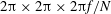
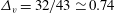
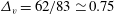
Figure 1. QG equilibrium states (with
 $n_{v}=83$
) at the ends of the solution branches where the vortices nearly touch for (a)
$n_{v}=83$
) at the ends of the solution branches where the vortices nearly touch for (a)
 $\unicode[STIX]{x1D6E5}_{v}=0$
, (b)
$\unicode[STIX]{x1D6E5}_{v}=0$
, (b)
 $\unicode[STIX]{x1D6E5}_{v}=11/83\simeq 1.1325$
, (c)
$\unicode[STIX]{x1D6E5}_{v}=11/83\simeq 1.1325$
, (c)
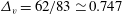
 $\unicode[STIX]{x1D6E5}_{v}=21/83\simeq 0.253$
, (d)
$\unicode[STIX]{x1D6E5}_{v}=21/83\simeq 0.253$
, (d)
 $\unicode[STIX]{x1D6E5}_{v}=41/83\simeq 0.494$
and (e)
$\unicode[STIX]{x1D6E5}_{v}=41/83\simeq 0.494$
and (e)
 $\unicode[STIX]{x1D6E5}_{v}=62/83\simeq 0.747$
. The vortices are shown in a reference frame whose vertical coordinate has been stretched by
$\unicode[STIX]{x1D6E5}_{v}=62/83\simeq 0.747$
. The vortices are shown in a reference frame whose vertical coordinate has been stretched by
 $N/f$
. Note that these QG solutions do not depend on the value of
$N/f$
. Note that these QG solutions do not depend on the value of
 $f/N$
when written as a function of
$f/N$
when written as a function of
 $x$
,
$x$
,
 $y$
and
$y$
and
 $Nz/f$
.
$Nz/f$
.
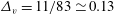
As originally suggested by Saffman & Szeto (Reference Saffman and Szeto1980) for two-dimensional vortices and verified in QG for three-dimensional vortices in Reinaud & Dritschel (Reference Reinaud and Dritschel2002) and Reinaud & Dritschel (Reference Reinaud and Dritschel2005), the margin of linear stability of the vortex equilibrium (which corresponds to the critical merger distance) coincides with the maximum of the total energy
 $E$
as a function of the gap
$E$
as a function of the gap
 $\unicode[STIX]{x1D6FF}$
between the vortices. It also coincides with the minimum of the angular impulse
$\unicode[STIX]{x1D6FF}$
between the vortices. It also coincides with the minimum of the angular impulse
 $J=\iiint q(x^{2}+y^{2})\,\text{d}V$
. Figure 2 shows the total energy
$J=\iiint q(x^{2}+y^{2})\,\text{d}V$
. Figure 2 shows the total energy
 $E(\unicode[STIX]{x1D6FF})$
for the five branches of solutions, distinguished by their value of
$E(\unicode[STIX]{x1D6FF})$
for the five branches of solutions, distinguished by their value of
 $\unicode[STIX]{x1D6E5}_{v}$
. As explained in Reinaud & Dritschel (Reference Reinaud and Dritschel2002), the total energy
$\unicode[STIX]{x1D6E5}_{v}$
. As explained in Reinaud & Dritschel (Reference Reinaud and Dritschel2002), the total energy
 $E$
first increases as the gap
$E$
first increases as the gap
 $\unicode[STIX]{x1D6FF}$
decreases as a consequence of the increase in the interaction energy. As the gap decreases further, however, the vortices become more deformed in response to the shear induced by their partner. The deformation decreases the self-energy of the vortices. For
$\unicode[STIX]{x1D6FF}$
decreases as a consequence of the increase in the interaction energy. As the gap decreases further, however, the vortices become more deformed in response to the shear induced by their partner. The deformation decreases the self-energy of the vortices. For
 $\unicode[STIX]{x1D6FF}<\unicode[STIX]{x1D6FF}_{c}$
, the energy decreases as
$\unicode[STIX]{x1D6FF}<\unicode[STIX]{x1D6FF}_{c}$
, the energy decreases as
 $\unicode[STIX]{x1D6FF}$
is further reduced as the latter effect becomes dominant.
$\unicode[STIX]{x1D6FF}$
is further reduced as the latter effect becomes dominant.
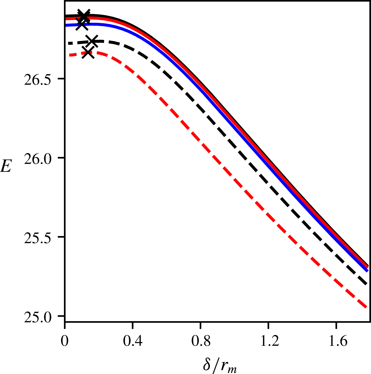
Figure 2. Total energy
 $E$
versus the gap
$E$
versus the gap
 $\unicode[STIX]{x1D6FF}$
for a vertical offset of
$\unicode[STIX]{x1D6FF}$
for a vertical offset of
 $\unicode[STIX]{x1D6E5}_{v}=0$
(solid black),
$\unicode[STIX]{x1D6E5}_{v}=0$
(solid black),
 $\unicode[STIX]{x1D6E5}_{v}=11/83\simeq 1.1325$
(solid red)
$\unicode[STIX]{x1D6E5}_{v}=11/83\simeq 1.1325$
(solid red)
 $\unicode[STIX]{x1D6E5}_{v}=21/83\simeq 0.253$
(solid blue),
$\unicode[STIX]{x1D6E5}_{v}=21/83\simeq 0.253$
(solid blue),
 $\unicode[STIX]{x1D6E5}_{v}=41/83\simeq 0.494$
(dashed black) and
$\unicode[STIX]{x1D6E5}_{v}=41/83\simeq 0.494$
(dashed black) and
 $\unicode[STIX]{x1D6E5}_{v}=62/83\simeq 0.747$
(dashed red). The symbol
$\unicode[STIX]{x1D6E5}_{v}=62/83\simeq 0.747$
(dashed red). The symbol
 $\times$
indicates the location of the energy maximum and coincides with the margin of linear stability.
$\times$
indicates the location of the energy maximum and coincides with the margin of linear stability.
The results described here provide initial conditions for the two vortices on both sides of the QG margin of stability, hence on both sides of the QG critical merger distance, for five different values of the vertical offset between the vortices.
4 Results
We next analyse two sets of non-hydrostatic simulations conducted to locate the critical merger distance for five different vertical offsets
 $\unicode[STIX]{x1D6E5}_{v}$
, as well as for various PV-based Rossby numbers
$\unicode[STIX]{x1D6E5}_{v}$
, as well as for various PV-based Rossby numbers
 $Ro_{PV}$
. As mentioned above, the two sets of simulations have different resolutions. Set I uses
$Ro_{PV}$
. As mentioned above, the two sets of simulations have different resolutions. Set I uses
 $n_{g}^{3}=128^{3}$
while set II uses
$n_{g}^{3}=128^{3}$
while set II uses
 $n_{g}^{3}=256^{3}$
. We have run in total over 100 simulations at
$n_{g}^{3}=256^{3}$
. We have run in total over 100 simulations at
 $128^{3}$
and 50 at
$128^{3}$
and 50 at
 $256^{3}$
for times up to
$256^{3}$
for times up to
 $t_{QG}=50$
. This time limit comes from extensive experience studying QG vortex interactions, and it is long enough to cover the onset and development of vortex merger.
$t_{QG}=50$
. This time limit comes from extensive experience studying QG vortex interactions, and it is long enough to cover the onset and development of vortex merger.
Set I considers
 $Ro_{PV}\in \{-0.8,-0.6,-0.5,-0.25,-0.1,0.1,0.25,0.5,0.75,1\}$
, while set II considers
$Ro_{PV}\in \{-0.8,-0.6,-0.5,-0.25,-0.1,0.1,0.25,0.5,0.75,1\}$
, while set II considers
 $Ro_{PV}\in \{-0.6,-0.5,-0.25,-0.1,0.1,0.25,0.5,0.75\}$
. The asymmetry between the values chosen for positive and negative
$Ro_{PV}\in \{-0.6,-0.5,-0.25,-0.1,0.1,0.25,0.5,0.75\}$
. The asymmetry between the values chosen for positive and negative
 $Ro_{PV}$
comes from the fact that anticyclones are more prone to static instability (see Tsang & Dritschel Reference Tsang and Dritschel2015). The numerical method assumes a bijective relation between isopycnal levels and physical heights, and simulations are stopped when static instability is detected. Moreover, such intense (local) events are more likely to be captured by high-resolution simulations.
$Ro_{PV}$
comes from the fact that anticyclones are more prone to static instability (see Tsang & Dritschel Reference Tsang and Dritschel2015). The numerical method assumes a bijective relation between isopycnal levels and physical heights, and simulations are stopped when static instability is detected. Moreover, such intense (local) events are more likely to be captured by high-resolution simulations.
The fact that anticyclones are more intense for a given value of PV
 $q$
can be traced back to the first ageostrophic correction in the equations of motion. Following McKiver & Dritschel (Reference McKiver and Dritschel2016), consider a single vortex of uniform PV anomaly
$q$
can be traced back to the first ageostrophic correction in the equations of motion. Following McKiver & Dritschel (Reference McKiver and Dritschel2016), consider a single vortex of uniform PV anomaly
 $q$
which is spherical in a reference frame whose vertical direction has been stretched by a factor
$q$
which is spherical in a reference frame whose vertical direction has been stretched by a factor
 $N/f$
, i.e.
$N/f$
, i.e.
 $z^{\ast }=Nz/f$
. Then, the interior vertical potential to
$z^{\ast }=Nz/f$
. Then, the interior vertical potential to
 $\mathit{O}(q^{2})$
is given by
$\mathit{O}(q^{2})$
is given by
 $$\begin{eqnarray}\unicode[STIX]{x1D719}=\frac{qr^{2}}{6}-\frac{q^{2}r^{2}}{27}+\frac{q^{2}r^{2}}{180}\left(\cos 2\unicode[STIX]{x1D703}-\frac{1}{3}\right),\end{eqnarray}$$
where
 $r=\sqrt{x^{2}+y^{2}+{z^{\ast }}^{2}}$
is the radial distance from the vortex centre and
$r=\sqrt{x^{2}+y^{2}+{z^{\ast }}^{2}}$
is the radial distance from the vortex centre and
 $\unicode[STIX]{x1D703}$
is the latitude. The exterior vertical potential is given by
$\unicode[STIX]{x1D703}$
is the latitude. The exterior vertical potential is given by
 $$\begin{eqnarray}\unicode[STIX]{x1D719}=-\frac{q}{3r}+\frac{q^{2}}{54r^{4}}+\left(\frac{q^{2}}{30r^{3}}-\frac{q^{2}}{36r^{4}}\right)\left(\cos 2\unicode[STIX]{x1D703}-\frac{1}{3}\right).\end{eqnarray}$$
The horizontal potentials vanish,
 $\unicode[STIX]{x1D753}_{h}=0$
. The first term in both equations is the well-known QG solution. The dominant correction term
$\unicode[STIX]{x1D753}_{h}=0$
. The first term in both equations is the well-known QG solution. The dominant correction term
 $-q^{2}r^{2}/27$
in (4.1) shows that
$-q^{2}r^{2}/27$
in (4.1) shows that
 $\unicode[STIX]{x1D719}$
increases in magnitude for anticyclones but decreases for cyclones. Overall, therefore, anticyclones are expected to be associated with higher values of vorticity
$\unicode[STIX]{x1D719}$
increases in magnitude for anticyclones but decreases for cyclones. Overall, therefore, anticyclones are expected to be associated with higher values of vorticity
 $\unicode[STIX]{x1D714}$
and buoyancy anomaly
$\unicode[STIX]{x1D714}$
and buoyancy anomaly
 $b$
.
$b$
.
Figure 3 summarises the results. The gap
 $\unicode[STIX]{x1D6FF}^{+}$
is the minimum gap for which no merger occurs by
$\unicode[STIX]{x1D6FF}^{+}$
is the minimum gap for which no merger occurs by
 $t_{QG}=50$
, while
$t_{QG}=50$
, while
 $\unicode[STIX]{x1D6FF}^{-}$
is the maximum gap for which merger occurs by this time. The difference between the two corresponds to the distance between two neighbouring solutions in our QG equilibrium database, and indicates the error range in our empirical determination of the critical merger distance.
$\unicode[STIX]{x1D6FF}^{-}$
is the maximum gap for which merger occurs by this time. The difference between the two corresponds to the distance between two neighbouring solutions in our QG equilibrium database, and indicates the error range in our empirical determination of the critical merger distance.
Figure 3. Critical merger gaps
 $\unicode[STIX]{x1D6FF}^{+}$
(solid) and
$\unicode[STIX]{x1D6FF}^{+}$
(solid) and
 $\unicode[STIX]{x1D6FF}^{-}$
(dotted) against the Rossby number
$\unicode[STIX]{x1D6FF}^{-}$
(dotted) against the Rossby number
 $Ro_{PV}$
. (a) Set I with
$Ro_{PV}$
. (a) Set I with
 $n_{g}^{3}=128^{3}$
and
$n_{g}^{3}=128^{3}$
and
 $\unicode[STIX]{x1D6E5}_{v}=0$
(black),
$\unicode[STIX]{x1D6E5}_{v}=0$
(black),
 $\unicode[STIX]{x1D6E5}_{v}=6/43\simeq 0.14$
(yellow),
$\unicode[STIX]{x1D6E5}_{v}=6/43\simeq 0.14$
(yellow),
 $\unicode[STIX]{x1D6E5}_{v}=11/43\simeq 0.26$
(red),
$\unicode[STIX]{x1D6E5}_{v}=11/43\simeq 0.26$
(red),
 $\unicode[STIX]{x1D6E5}_{v}=21/43\simeq 0.49$
(blue) and
$\unicode[STIX]{x1D6E5}_{v}=21/43\simeq 0.49$
(blue) and
 $\unicode[STIX]{x1D6E5}_{v}=32/43\simeq 0.74$
(green). (b) Set II with
$\unicode[STIX]{x1D6E5}_{v}=32/43\simeq 0.74$
(green). (b) Set II with
 $n_{g}^{3}=256^{3}$
and
$n_{g}^{3}=256^{3}$
and
 $\unicode[STIX]{x1D6E5}_{v}=0$
(black),
$\unicode[STIX]{x1D6E5}_{v}=0$
(black),
 $\unicode[STIX]{x1D6E5}_{v}=11/83\simeq 0.13$
(yellow),
$\unicode[STIX]{x1D6E5}_{v}=11/83\simeq 0.13$
(yellow),
 $\unicode[STIX]{x1D6E5}_{v}=21/83\simeq 0.25$
(red),
$\unicode[STIX]{x1D6E5}_{v}=21/83\simeq 0.25$
(red),
 $\unicode[STIX]{x1D6E5}_{v}=41/83\simeq 0.5$
(blue) and
$\unicode[STIX]{x1D6E5}_{v}=41/83\simeq 0.5$
(blue) and
 $\unicode[STIX]{x1D6E5}_{v}=62/83\simeq 0.75$
(green). The outcome is based on simulations run up to
$\unicode[STIX]{x1D6E5}_{v}=62/83\simeq 0.75$
(green). The outcome is based on simulations run up to
 $t_{QG}=50$
.
$t_{QG}=50$
.
There is a large influence of the spatial resolution on the results. As a consequence, we cannot confirm that set II has reached convergence. Robust trends can nonetheless be identified from the results. First, we note that the gaps
 $\unicode[STIX]{x1D6FF}^{\pm }$
tend to increase for large values of
$\unicode[STIX]{x1D6FF}^{\pm }$
tend to increase for large values of
 $|Ro_{PV}|$
. This can be explained by the increased importance of ageostrophic effects (discussed below). Second, we observe an asymmetry for
$|Ro_{PV}|$
. This can be explained by the increased importance of ageostrophic effects (discussed below). Second, we observe an asymmetry for
 $\unicode[STIX]{x1D6FF}^{\pm }$
between the cases with positive
$\unicode[STIX]{x1D6FF}^{\pm }$
between the cases with positive
 $Ro_{PV}$
and those with negative
$Ro_{PV}$
and those with negative
 $Ro_{PV}$
. For small values of
$Ro_{PV}$
. For small values of
 $\unicode[STIX]{x1D6E5}_{v}$
, when the vortices are nearly aligned horizontally, cyclones with
$\unicode[STIX]{x1D6E5}_{v}$
, when the vortices are nearly aligned horizontally, cyclones with
 $Ro_{PV}=\unicode[STIX]{x1D716}>0$
tend to be able to merge from larger gaps
$Ro_{PV}=\unicode[STIX]{x1D716}>0$
tend to be able to merge from larger gaps
 $\unicode[STIX]{x1D6FF}$
than their anticyclonic counterparts with
$\unicode[STIX]{x1D6FF}$
than their anticyclonic counterparts with
 $Ro_{PV}=-\unicode[STIX]{x1D716}<0$
. In particular, anticyclones do not merge even when the vortices initially nearly touch at
$Ro_{PV}=-\unicode[STIX]{x1D716}<0$
. In particular, anticyclones do not merge even when the vortices initially nearly touch at
 $t=0$
for
$t=0$
for
 $-0.5\leqslant Ro_{PV}\leqslant -0.1$
at resolution
$-0.5\leqslant Ro_{PV}\leqslant -0.1$
at resolution
 $256^{3}$
. Notably, the vertical shear that one vortex induces on the other is small for small values of
$256^{3}$
. Notably, the vertical shear that one vortex induces on the other is small for small values of
 $\unicode[STIX]{x1D6E5}_{v}$
.
$\unicode[STIX]{x1D6E5}_{v}$
.
The trend is, however, reversed for larger values of
 $\unicode[STIX]{x1D6E5}_{v}$
. Then, the vertical shear induced by one vortex on the other is enhanced and anticyclones appear to be able to merge for larger
$\unicode[STIX]{x1D6E5}_{v}$
. Then, the vertical shear induced by one vortex on the other is enhanced and anticyclones appear to be able to merge for larger
 $\unicode[STIX]{x1D6FF}$
than cyclones at the same
$\unicode[STIX]{x1D6FF}$
than cyclones at the same
 $Ro_{PV}$
. This suggests a competition between two opposing effects. The effects appear to balance around
$Ro_{PV}$
. This suggests a competition between two opposing effects. The effects appear to balance around
 $\unicode[STIX]{x1D6E5}_{v}\sim 0.25$
where the curve
$\unicode[STIX]{x1D6E5}_{v}\sim 0.25$
where the curve
 $\unicode[STIX]{x1D6FF}^{\pm }$
against
$\unicode[STIX]{x1D6FF}^{\pm }$
against
 $Ro_{PV}$
is almost symmetric across the axis
$Ro_{PV}$
is almost symmetric across the axis
 $Ro_{PV}=0$
.
$Ro_{PV}=0$
.
To help understand these results, consider the time evolution of the distance
 $d$
between the vortices and of their shape, along with the time evolution of the ageostrophic energy. The distance between the vortices is obtained by determining the location of the centroid of each vortex (identified as contiguous volumes of uniform PV). The centroid position of vortex
$d$
between the vortices and of their shape, along with the time evolution of the ageostrophic energy. The distance between the vortices is obtained by determining the location of the centroid of each vortex (identified as contiguous volumes of uniform PV). The centroid position of vortex
 $k$
occupying the volume
$k$
occupying the volume
 $V^{k}$
is simply
$V^{k}$
is simply
 $\boldsymbol{x}_{v}^{k}=\iiint _{V^{k}}(x,y,z^{\ast })\,\text{d}V/\iiint _{V^{k}}\text{d}V$
. (The integration is done by contour integration.) For the sake of simplicity, the generally weak variation in height between neighbouring isopycnals (and the contours lying on them) is not taken into account but is assumed constant in this diagnostic.
$\boldsymbol{x}_{v}^{k}=\iiint _{V^{k}}(x,y,z^{\ast })\,\text{d}V/\iiint _{V^{k}}\text{d}V$
. (The integration is done by contour integration.) For the sake of simplicity, the generally weak variation in height between neighbouring isopycnals (and the contours lying on them) is not taken into account but is assumed constant in this diagnostic.
To characterise the shape of the vortices, we first determine the ellipsoids that best fit them. In particular, we determine the semi-axis lengths of the best-fit ellipsoids and analyse their time evolution as the vortices deform. The ‘best-fit ellipsoid’ is the one having the same volume, centroid and second-order spatial moments. The latter are defined for vortex
 $k$
in terms of a symmetric
$k$
in terms of a symmetric
 $3\times 3$
matrix:
$3\times 3$
matrix:
 $$\begin{eqnarray}{\mathcal{B}}^{k}=[B_{i,j}^{k}],\quad B_{i,j}^{k}=\frac{5}{V^{k}}\iiint _{V^{k}}\tilde{x}_{i}^{k}\tilde{x}_{j}^{k}\,\text{d}V,\end{eqnarray}$$
where
 $\tilde{\boldsymbol{x}}^{k}=(\tilde{x}_{1}^{k},\tilde{x}_{2}^{k},\tilde{x}_{3}^{k})=(x-x_{v}^{k},y-y_{v}^{k},z^{\ast }-z_{v}^{k})$
. The equation for the best-fit ellipsoid surface is then
$\tilde{\boldsymbol{x}}^{k}=(\tilde{x}_{1}^{k},\tilde{x}_{2}^{k},\tilde{x}_{3}^{k})=(x-x_{v}^{k},y-y_{v}^{k},z^{\ast }-z_{v}^{k})$
. The equation for the best-fit ellipsoid surface is then
 $$\begin{eqnarray}\tilde{\boldsymbol{x}}^{k}{{\mathcal{B}}^{k}}^{-1}\tilde{\boldsymbol{x}}^{kT}=1.\end{eqnarray}$$
The eigenvalues of the matrix
 ${\mathcal{B}}^{k}$
are the squared semi-axes lengths
${\mathcal{B}}^{k}$
are the squared semi-axes lengths
 $(a^{2},b^{2},c^{2})$
of the ellipsoid. We sort the semi-axes lengths such that
$(a^{2},b^{2},c^{2})$
of the ellipsoid. We sort the semi-axes lengths such that
 $a\leqslant b\leqslant c$
without loss of generality. We denote
$a\leqslant b\leqslant c$
without loss of generality. We denote
 $(a_{0},b_{0},c_{0})$
as their values at
$(a_{0},b_{0},c_{0})$
as their values at
 $t=0$
. Note that, owing to the symmetry of the initial conditions, both vortices behave in a similar way. We thus only present results for one of the two vortices, or for the largest vortex if the interaction results in a change in the number of identifiable vortices.
$t=0$
. Note that, owing to the symmetry of the initial conditions, both vortices behave in a similar way. We thus only present results for one of the two vortices, or for the largest vortex if the interaction results in a change in the number of identifiable vortices.
To diagnose the ageostrophic energy and other ageostrophic features of the flow, we determine the balanced part of the vector potential
 $\unicode[STIX]{x1D753}$
using two different balance conditions. In the first one, we decompose the full potential
$\unicode[STIX]{x1D753}$
using two different balance conditions. In the first one, we decompose the full potential
 $\unicode[STIX]{x1D753}$
at time
$\unicode[STIX]{x1D753}$
at time
 $t$
as the sum of a QG potential
$t$
as the sum of a QG potential
 $\unicode[STIX]{x1D753}_{QG}$
and an ageostrophic part, simply defined as the departure of the full potential from the QG potential,
$\unicode[STIX]{x1D753}_{QG}$
and an ageostrophic part, simply defined as the departure of the full potential from the QG potential,
 $\unicode[STIX]{x1D753}_{ageo}\equiv \unicode[STIX]{x1D753}-\unicode[STIX]{x1D753}_{QG}$
. The QG potential
$\unicode[STIX]{x1D753}_{ageo}\equiv \unicode[STIX]{x1D753}-\unicode[STIX]{x1D753}_{QG}$
. The QG potential
 $\unicode[STIX]{x1D753}_{QG}=(0,0,\unicode[STIX]{x1D719}_{QG})$
is obtained, at any given time
$\unicode[STIX]{x1D753}_{QG}=(0,0,\unicode[STIX]{x1D719}_{QG})$
is obtained, at any given time
 $t$
, by taking the PV distribution from the non-hydrostatic simulation and inverting
$t$
, by taking the PV distribution from the non-hydrostatic simulation and inverting
 ${\mathcal{L}}_{QG}(\unicode[STIX]{x1D719}_{QG})=q$
. The second balance condition used is the nonlinear QG (NQG) balance introduced in McKiver & Dritschel (Reference McKiver and Dritschel2008). The balance relations include the ageostrophic corrections up to
${\mathcal{L}}_{QG}(\unicode[STIX]{x1D719}_{QG})=q$
. The second balance condition used is the nonlinear QG (NQG) balance introduced in McKiver & Dritschel (Reference McKiver and Dritschel2008). The balance relations include the ageostrophic corrections up to
 ${\mathcal{O}}(Ro_{PV}^{2})$
. Details of the balance condition may be found in McKiver & Dritschel (Reference McKiver and Dritschel2008) and Tsang & Dritschel (Reference Tsang and Dritschel2015), and are not reproduced here. The diagnosis of the NQG-balanced part
${\mathcal{O}}(Ro_{PV}^{2})$
. Details of the balance condition may be found in McKiver & Dritschel (Reference McKiver and Dritschel2008) and Tsang & Dritschel (Reference Tsang and Dritschel2015), and are not reproduced here. The diagnosis of the NQG-balanced part
 $\unicode[STIX]{x1D753}_{NQG}$
allows us to estimate the imbalanced part of the fields, namely
$\unicode[STIX]{x1D753}_{NQG}$
allows us to estimate the imbalanced part of the fields, namely
 $\unicode[STIX]{x1D753}_{imb}=\unicode[STIX]{x1D753}-\unicode[STIX]{x1D753}_{NQG}$
. It should be noted that the ‘imbalanced’ part of the potential
$\unicode[STIX]{x1D753}_{imb}=\unicode[STIX]{x1D753}-\unicode[STIX]{x1D753}_{NQG}$
. It should be noted that the ‘imbalanced’ part of the potential
 $\unicode[STIX]{x1D753}_{imb}$
is included in the ageostrophic part
$\unicode[STIX]{x1D753}_{imb}$
is included in the ageostrophic part
 $\unicode[STIX]{x1D753}_{ageo}$
. These potentials allow one to define the associated velocities and buoyancy anomalies from (2.5) and (2.6).
$\unicode[STIX]{x1D753}_{ageo}$
. These potentials allow one to define the associated velocities and buoyancy anomalies from (2.5) and (2.6).
We next define the (scaled) energies from either
 $\unicode[STIX]{x1D753}^{\prime }=\unicode[STIX]{x1D753}$
or
$\unicode[STIX]{x1D753}^{\prime }=\unicode[STIX]{x1D753}$
or
 $\unicode[STIX]{x1D753}_{ageo}$
or
$\unicode[STIX]{x1D753}_{ageo}$
or
 $\unicode[STIX]{x1D753}_{imb}$
as follows:
$\unicode[STIX]{x1D753}_{imb}$
as follows:
 $$\begin{eqnarray}E^{\prime }=\iiint _{D}\left(|\unicode[STIX]{x1D735}\times \unicode[STIX]{x1D753}^{\prime }|^{2}+\left({\displaystyle \frac{\unicode[STIX]{x1D735}\boldsymbol{\cdot }\unicode[STIX]{x1D753}^{\prime }}{N}}\right)^{2}\right)\,\text{d}V.\end{eqnarray}$$
The first term in the integral represents the kinetic energy (rescaled by
 $f^{2}$
) and the second term represents the scaled potential energy (proportional to the squared buoyancy anomaly).
$f^{2}$
) and the second term represents the scaled potential energy (proportional to the squared buoyancy anomaly).
At
 $t=0$
, the vortices are in near-equilibrium and in a near-balanced state. Yet, they contain a small amount of imbalance, and they spontaneously emit a small amount of inertia–gravity waves (IGWs). The presence of IGWs can be inferred by the spatial pattern of the imbalanced vertical velocity field,
$t=0$
, the vortices are in near-equilibrium and in a near-balanced state. Yet, they contain a small amount of imbalance, and they spontaneously emit a small amount of inertia–gravity waves (IGWs). The presence of IGWs can be inferred by the spatial pattern of the imbalanced vertical velocity field,
 $w_{imb}=-f\unicode[STIX]{x1D735}\times \unicode[STIX]{x1D753}_{imb}\boldsymbol{\cdot }\boldsymbol{k}$
, where
$w_{imb}=-f\unicode[STIX]{x1D735}\times \unicode[STIX]{x1D753}_{imb}\boldsymbol{\cdot }\boldsymbol{k}$
, where
 $\boldsymbol{k}$
is the vertical unit vector. Figure 4 shows cross-sections of
$\boldsymbol{k}$
is the vertical unit vector. Figure 4 shows cross-sections of
 $w_{imb}$
for
$w_{imb}$
for
 $\unicode[STIX]{x1D6E5}_{v}=0$
,
$\unicode[STIX]{x1D6E5}_{v}=0$
,
 $Ro_{PV}=-0.5$
and
$Ro_{PV}=-0.5$
and
 $\unicode[STIX]{x1D6FF}/r_{m}=0.5$
at resolution
$\unicode[STIX]{x1D6FF}/r_{m}=0.5$
at resolution
 $256^{3}$
(set II). The patterns observed in this case are qualitatively representative of the patterns observed in all other cases. The vertical cross-sections show the characteristic Saint Andrew’s cross pattern of IGWs as they disperse away from the vortices. Moreover, as the two vortices co-rotate, the IGWs spread away from the vortices in a spiral pattern. Similar spiral patterns have been observed by Viúdez (Reference Viúdez2006) and Pallàs-Sanz & Viúdez (Reference Pallàs-Sanz and Viúdez2008). The maximum imbalanced vertical velocities are found inside the vortex, in particular near their inner edges. These are the parts of the vortices which interact most strongly. As the vortices lose energy to waves, they deform and further depart from their initial near-equilibrium configuration. The interaction is also accompanied by increased ageostrophic motion.
$256^{3}$
(set II). The patterns observed in this case are qualitatively representative of the patterns observed in all other cases. The vertical cross-sections show the characteristic Saint Andrew’s cross pattern of IGWs as they disperse away from the vortices. Moreover, as the two vortices co-rotate, the IGWs spread away from the vortices in a spiral pattern. Similar spiral patterns have been observed by Viúdez (Reference Viúdez2006) and Pallàs-Sanz & Viúdez (Reference Pallàs-Sanz and Viúdez2008). The maximum imbalanced vertical velocities are found inside the vortex, in particular near their inner edges. These are the parts of the vortices which interact most strongly. As the vortices lose energy to waves, they deform and further depart from their initial near-equilibrium configuration. The interaction is also accompanied by increased ageostrophic motion.

Figure 4. Cross-section of the imbalanced vertical velocity
 $w_{imb}=-f\unicode[STIX]{x1D735}\times \unicode[STIX]{x1D753}_{imb}\boldsymbol{\cdot }\boldsymbol{k}$
for a
$w_{imb}=-f\unicode[STIX]{x1D735}\times \unicode[STIX]{x1D753}_{imb}\boldsymbol{\cdot }\boldsymbol{k}$
for a
 $256^{3}$
simulation with
$256^{3}$
simulation with
 $\unicode[STIX]{x1D6E5}_{v}=0$
,
$\unicode[STIX]{x1D6E5}_{v}=0$
,
 $Ro_{PV}=-0.5$
and
$Ro_{PV}=-0.5$
and
 $\unicode[STIX]{x1D6FF}/r_{m}=0.5$
. (a,b) Vertical cross-section in the mid-plane
$\unicode[STIX]{x1D6FF}/r_{m}=0.5$
. (a,b) Vertical cross-section in the mid-plane
 $x=0$
at
$x=0$
at
 $t_{QG}=2$
(a) and
$t_{QG}=2$
(a) and
 $3$
(b). (c,d) Horizontal cross-section in the mid-plane
$3$
(b). (c,d) Horizontal cross-section in the mid-plane
 $z=0$
at
$z=0$
at
 $t=11$
(c) and
$t=11$
(c) and
 $t=12$
(d). The colour map is bounded to better visualise the waves spreading away from the vortices.
$t=12$
(d). The colour map is bounded to better visualise the waves spreading away from the vortices.
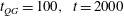
The total energy (derived from
 $\unicode[STIX]{x1D753}^{\prime }=\unicode[STIX]{x1D753}$
in (4.5)) is conserved for an adiabatic inviscid flow. With weak biharmonic diffusion, the total energy is nearly conserved, within the accuracy of its calculation on the inversion grid. We focus on the time evolution of the ageostrophic energy
$\unicode[STIX]{x1D753}^{\prime }=\unicode[STIX]{x1D753}$
in (4.5)) is conserved for an adiabatic inviscid flow. With weak biharmonic diffusion, the total energy is nearly conserved, within the accuracy of its calculation on the inversion grid. We focus on the time evolution of the ageostrophic energy
 $E_{ageo}$
obtained from the potential
$E_{ageo}$
obtained from the potential
 $\unicode[STIX]{x1D753}^{\prime }=\unicode[STIX]{x1D753}_{ageo}=\unicode[STIX]{x1D753}-\unicode[STIX]{x1D753}_{QG}$
in (4.5). Figure 5 shows
$\unicode[STIX]{x1D753}^{\prime }=\unicode[STIX]{x1D753}_{ageo}=\unicode[STIX]{x1D753}-\unicode[STIX]{x1D753}_{QG}$
in (4.5). Figure 5 shows
 $E_{ageo}$
, for two cases at resolution
$E_{ageo}$
, for two cases at resolution
 $256^{3}$
,
$256^{3}$
,
 $\unicode[STIX]{x1D6E5}_{v}=0$
and
$\unicode[STIX]{x1D6E5}_{v}=0$
and
 $\unicode[STIX]{x1D6FF}/r_{m}=0.5$
, specifically for
$\unicode[STIX]{x1D6FF}/r_{m}=0.5$
, specifically for
 $Ro_{PV}=0.5$
and
$Ro_{PV}=0.5$
and
 $Ro_{PV}=-0.5$
. The vortices do not merge, allowing us to explore the time evolution of the individual vortices over a large time period. For these two particular simulations, diagnostics are obtained over an extended time period, up to
$Ro_{PV}=-0.5$
. The vortices do not merge, allowing us to explore the time evolution of the individual vortices over a large time period. For these two particular simulations, diagnostics are obtained over an extended time period, up to
 $t_{QG}=100$
, that is,
$t_{QG}=100$
, that is,
 $t=2000$
. First, we see that
$t=2000$
. First, we see that
 $E_{ageo}$
is typically larger for anticyclones than for cyclones. This is consistent with the fact that anticyclones are more intense than cyclones for a given
$E_{ageo}$
is typically larger for anticyclones than for cyclones. This is consistent with the fact that anticyclones are more intense than cyclones for a given
 $|Ro_{PV}|$
. We also see that, overall,
$|Ro_{PV}|$
. We also see that, overall,
 $E_{ageo}$
decreases with time for cyclones, with small-amplitude oscillations, while it increases for anticyclones.
$E_{ageo}$
decreases with time for cyclones, with small-amplitude oscillations, while it increases for anticyclones.
We can relate these general trends to the time evolution of the distance
 $d$
separating the two vortex centroids, also presented in figure 5. Cyclones tend to move towards one another while anticyclones move away from each other. For anticyclones the ageostrophic motion extracts energy from the QG balanced energy. This means that the vortices move further apart to remain in near-equilibrium, consistent with figure 2. It should be noted that this equivalence is not straightforward, as the energy is a quadratic quantity. The full, conserved, energy
$d$
separating the two vortex centroids, also presented in figure 5. Cyclones tend to move towards one another while anticyclones move away from each other. For anticyclones the ageostrophic motion extracts energy from the QG balanced energy. This means that the vortices move further apart to remain in near-equilibrium, consistent with figure 2. It should be noted that this equivalence is not straightforward, as the energy is a quadratic quantity. The full, conserved, energy
 $E$
associated with
$E$
associated with
 $\unicode[STIX]{x1D753}$
is not the sum of the energy
$\unicode[STIX]{x1D753}$
is not the sum of the energy
 $E_{QG}$
associated with
$E_{QG}$
associated with
 $\unicode[STIX]{x1D753}_{QG}$
and the energy
$\unicode[STIX]{x1D753}_{QG}$
and the energy
 $E_{ageo}$
associated with the ageostrophic potential
$E_{ageo}$
associated with the ageostrophic potential
 $\unicode[STIX]{x1D753}_{ageo}=\unicode[STIX]{x1D753}-\unicode[STIX]{x1D753}_{QG}$
. We can nonetheless infer that anticyclones separate due to a transfer of energy from the QG balanced part of the flow to the ageostrophic part. On the other hand, we deduce that cyclones merge from further apart compared to anticyclones because some energy is transferred from
$\unicode[STIX]{x1D753}_{ageo}=\unicode[STIX]{x1D753}-\unicode[STIX]{x1D753}_{QG}$
. We can nonetheless infer that anticyclones separate due to a transfer of energy from the QG balanced part of the flow to the ageostrophic part. On the other hand, we deduce that cyclones merge from further apart compared to anticyclones because some energy is transferred from
 $E_{ageo}$
to
$E_{ageo}$
to
 $E_{QG}$
and this results in the vortices moving closer together.
$E_{QG}$
and this results in the vortices moving closer together.
Figure 5. (a,b) Evolution of the ageostrophic energy
 $E_{ageo}$
for two
$E_{ageo}$
for two
 $256^{3}$
simulations with
$256^{3}$
simulations with
 $\unicode[STIX]{x1D6E5}_{v}=0$
,
$\unicode[STIX]{x1D6E5}_{v}=0$
,
 $\unicode[STIX]{x1D6FF}/r_{m}=0.5$
and
$\unicode[STIX]{x1D6FF}/r_{m}=0.5$
and
 $Ro_{PV}=0.5$
(a) and
$Ro_{PV}=0.5$
(a) and
 $Ro_{PV}=-0.5$
(b). (c) Evolution of the distance
$Ro_{PV}=-0.5$
(b). (c) Evolution of the distance
 $d$
between the vortex centroids for
$d$
between the vortex centroids for
 $Ro_{PV}=0.5$
(black) and
$Ro_{PV}=0.5$
(black) and
 $Ro_{PV}=-0.5$
(red). (d) Evolution of the best-fit ellipsoid. Black lines corresponds to
$Ro_{PV}=-0.5$
(red). (d) Evolution of the best-fit ellipsoid. Black lines corresponds to
 $Ro_{PV}=0.5$
, and red lines to
$Ro_{PV}=0.5$
, and red lines to
 $Ro_{PV}=-0.5$
. The quantities plotted are
$Ro_{PV}=-0.5$
. The quantities plotted are
 $a/a_{0}$
(solid),
$a/a_{0}$
(solid),
 $b/b_{0}$
(dotted) and
$b/b_{0}$
(dotted) and
 $c/c_{0}$
(dashed).
$c/c_{0}$
(dashed).
Figure 6. Evolution of the vortices, depicted by their bounding contours in each isopycnal, and in a reference frame stretched in the vertical direction by
 $N/f$
, for
$N/f$
, for
 $\unicode[STIX]{x1D6E5}_{v}=0$
,
$\unicode[STIX]{x1D6E5}_{v}=0$
,
 $Ro_{PV}=0.5$
and
$Ro_{PV}=0.5$
and
 $\unicode[STIX]{x1D6FF}/r_{m}=0.5$
. The view is orthographic at an angle of
$\unicode[STIX]{x1D6FF}/r_{m}=0.5$
. The view is orthographic at an angle of
 $60^{\circ }$
from the vertical. Times displayed are (a)
$60^{\circ }$
from the vertical. Times displayed are (a)
 $t_{QG}=40,~t=800$
, (b)
$t_{QG}=40,~t=800$
, (b)
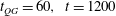 $t_{QG}=60,~t=1200$
and (c)
$t_{QG}=60,~t=1200$
and (c)
 $t_{QG}=100,~t=2000$
.
$t_{QG}=100,~t=2000$
.
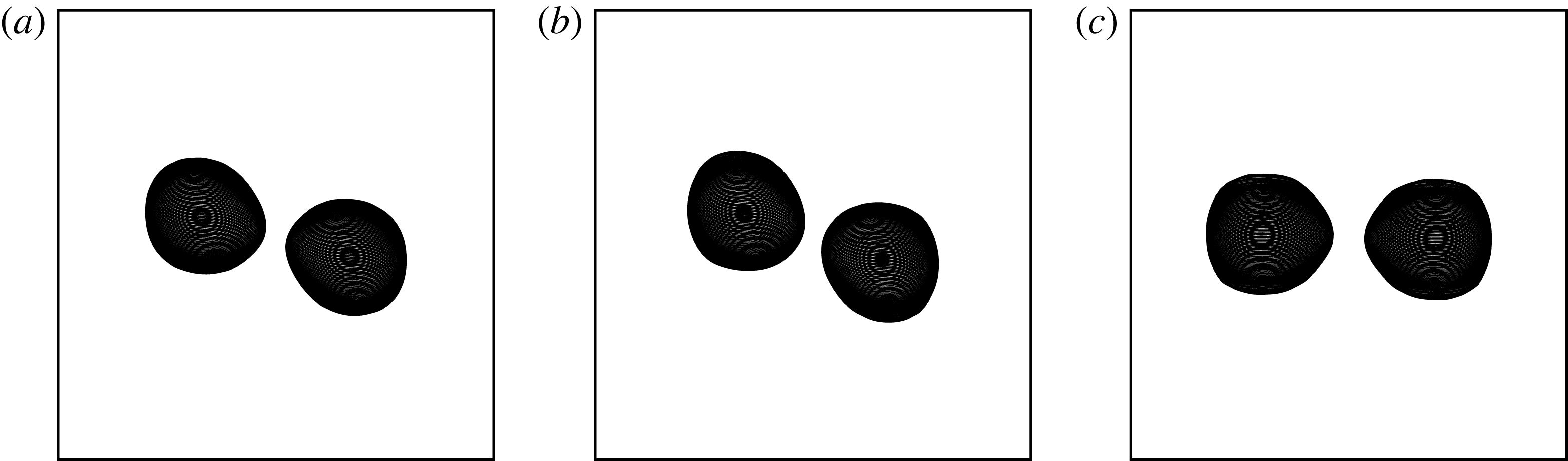
Figure 7. Evolution of the vortices, depicted by their bounding contours in each isopycnal, and in a reference frame stretched in the vertical direction by
 $N/f$
, for
$N/f$
, for
 $\unicode[STIX]{x1D6E5}_{v}=0$
,
$\unicode[STIX]{x1D6E5}_{v}=0$
,
 $Ro_{PV}=-0.5$
and
$Ro_{PV}=-0.5$
and
 $\unicode[STIX]{x1D6FF}/r_{m}=0.5$
. The view is orthographic at an angle of
$\unicode[STIX]{x1D6FF}/r_{m}=0.5$
. The view is orthographic at an angle of
 $60^{\circ }$
from the vertical. Times displayed are (a)
$60^{\circ }$
from the vertical. Times displayed are (a)
 $t_{QG}=31,~t=620$
, (b)
$t_{QG}=31,~t=620$
, (b)
 $t_{QG}=60,~t=1200$
and (c)
$t_{QG}=60,~t=1200$
and (c)
 $t_{QG}=100,~t=2000$
.
$t_{QG}=100,~t=2000$
.
Figure 8. (a,b) Evolution of the ageostrophic energy
 $E_{ageo}$
for two
$E_{ageo}$
for two
 $256^{3}$
simulations with
$256^{3}$
simulations with
 $\unicode[STIX]{x1D6E5}_{v}=21/83$
,
$\unicode[STIX]{x1D6E5}_{v}=21/83$
,
 $\unicode[STIX]{x1D6FF}/r_{m}=0.48$
and
$\unicode[STIX]{x1D6FF}/r_{m}=0.48$
and
 $Ro_{PV}=0.5$
(a) and
$Ro_{PV}=0.5$
(a) and
 $Ro_{PV}=-0.5$
(b). (c) Evolution of the distance
$Ro_{PV}=-0.5$
(b). (c) Evolution of the distance
 $d$
between the vortex centroids for
$d$
between the vortex centroids for
 $Ro_{PV}=0.5$
(black) and
$Ro_{PV}=0.5$
(black) and
 $Ro_{PV}=-0.5$
(red). (d) Evolution of the best-fit ellipsoid. Black lines represent results for
$Ro_{PV}=-0.5$
(red). (d) Evolution of the best-fit ellipsoid. Black lines represent results for
 $Ro_{PV}=0.5$
, red lines for
$Ro_{PV}=0.5$
, red lines for
 $Ro_{PV}=-0.5$
. The quantities plotted are
$Ro_{PV}=-0.5$
. The quantities plotted are
 $a/a_{0}$
(solid),
$a/a_{0}$
(solid),
 $b/b_{0}$
(dotted) and
$b/b_{0}$
(dotted) and
 $c/c_{0}$
(dashed).
$c/c_{0}$
(dashed).
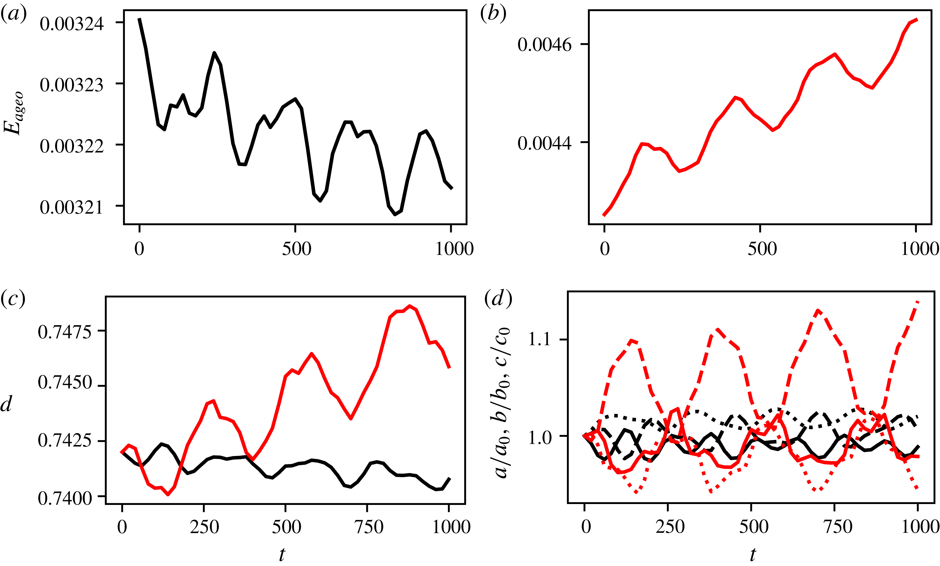
Figure 9. (a,b) Evolution of the ageostrophic energy
 $E_{ageo}$
for two
$E_{ageo}$
for two
 $256^{3}$
simulations with
$256^{3}$
simulations with
 $\unicode[STIX]{x1D6E5}_{v}=41/83$
,
$\unicode[STIX]{x1D6E5}_{v}=41/83$
,
 $\unicode[STIX]{x1D6FF}/r_{m}=0.62$
and
$\unicode[STIX]{x1D6FF}/r_{m}=0.62$
and
 $Ro_{PV}=0.5$
(a) and
$Ro_{PV}=0.5$
(a) and
 $Ro_{PV}=-0.5$
(b). (c) Evolution of the distance
$Ro_{PV}=-0.5$
(b). (c) Evolution of the distance
 $d$
between the vortex centroids for
$d$
between the vortex centroids for
 $Ro_{PV}=0.5$
(black) and
$Ro_{PV}=0.5$
(black) and
 $Ro_{PV}=-0.5$
(red). (d) Evolution of the best-fit ellipsoid. Black lines represent results for
$Ro_{PV}=-0.5$
(red). (d) Evolution of the best-fit ellipsoid. Black lines represent results for
 $Ro_{PV}=0.5$
, red lines for
$Ro_{PV}=0.5$
, red lines for
 $Ro_{PV}=-0.5$
. The quantities plotted are
$Ro_{PV}=-0.5$
. The quantities plotted are
 $a/a_{0}$
(solid),
$a/a_{0}$
(solid),
 $b/b_{0}$
(dotted) and
$b/b_{0}$
(dotted) and
 $c/c_{0}$
(dashed).
$c/c_{0}$
(dashed).

Figure 10. (a,b) Evolution of the ageostrophic
 $E_{ageo}$
for two
$E_{ageo}$
for two
 $256^{3}$
simulations with
$256^{3}$
simulations with
 $\unicode[STIX]{x1D6E5}_{v}=62/83$
,
$\unicode[STIX]{x1D6E5}_{v}=62/83$
,
 $\unicode[STIX]{x1D6FF}/r_{m}=0.55$
and
$\unicode[STIX]{x1D6FF}/r_{m}=0.55$
and
 $Ro_{PV}=0.5$
(a) and
$Ro_{PV}=0.5$
(a) and
 $Ro_{PV}=-0.5$
(b). (c) Evolution of the distance
$Ro_{PV}=-0.5$
(b). (c) Evolution of the distance
 $d$
between the vortex centroids for
$d$
between the vortex centroids for
 $Ro_{PV}=0.5$
(black) and
$Ro_{PV}=0.5$
(black) and
 $Ro_{PV}=-0.5$
(red). (d) Evolution of the best-fit ellipsoid. Black lines represent results for
$Ro_{PV}=-0.5$
(red). (d) Evolution of the best-fit ellipsoid. Black lines represent results for
 $Ro_{PV}=0.5$
, red lines for
$Ro_{PV}=0.5$
, red lines for
 $Ro_{PV}=-0.5$
. The quantities plotted are
$Ro_{PV}=-0.5$
. The quantities plotted are
 $a/a_{0}$
(solid),
$a/a_{0}$
(solid),
 $b/b_{0}$
(dotted) and
$b/b_{0}$
(dotted) and
 $c/c_{0}$
(dashed).
$c/c_{0}$
(dashed).
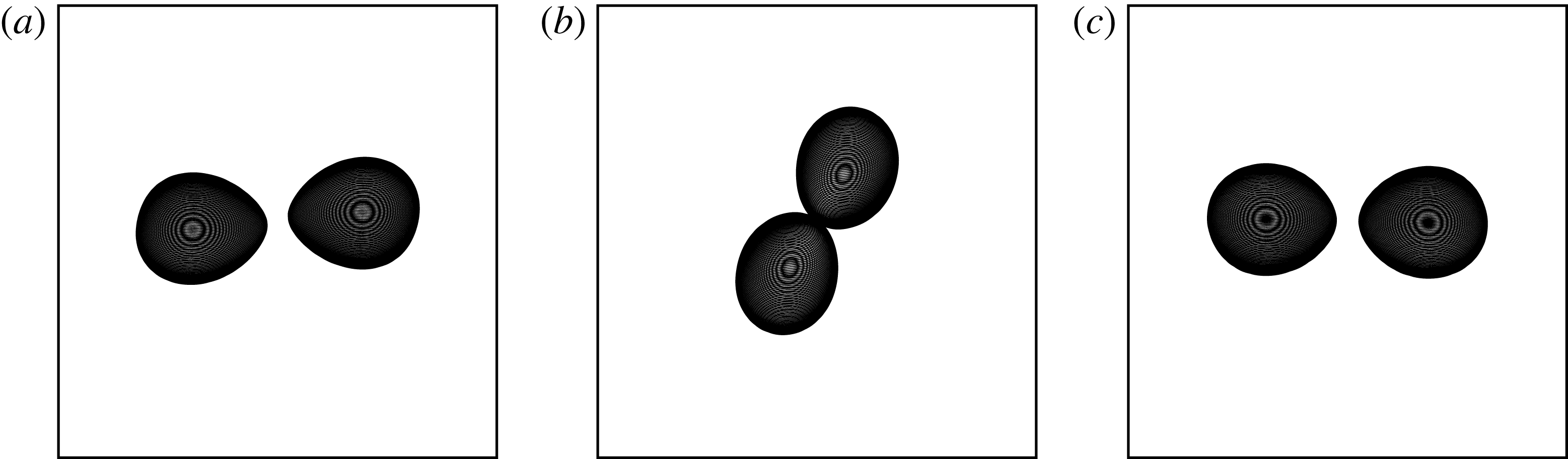
Figure 11. Evolution of the vortices, depicted by their bounding contours in each isopycnal, and in a reference frame stretched in the vertical direction by
 $N/f$
, for
$N/f$
, for
 $\unicode[STIX]{x1D6E5}_{v}=21/83$
,
$\unicode[STIX]{x1D6E5}_{v}=21/83$
,
 $Ro_{PV}=0.5$
and
$Ro_{PV}=0.5$
and
 $\unicode[STIX]{x1D6FF}/r_{m}=0.48$
. The view is orthographic at an angle of
$\unicode[STIX]{x1D6FF}/r_{m}=0.48$
. The view is orthographic at an angle of
 $60^{\circ }$
from the vertical. Times displayed are (a)
$60^{\circ }$
from the vertical. Times displayed are (a)
 $t_{QG}=21,~t=420$
, (b)
$t_{QG}=21,~t=420$
, (b)
 $t_{QG}=30,~t=600$
and (c)
$t_{QG}=30,~t=600$
and (c)
 $t_{QG}=45,~t=900$
.
$t_{QG}=45,~t=900$
.

Figure 12. Evolution of the vortices, depicted by their bounding contours in each isopycnal, and in a reference frame stretched in the vertical direction by
 $N/f$
, for
$N/f$
, for
 $\unicode[STIX]{x1D6E5}_{v}=21/83$
,
$\unicode[STIX]{x1D6E5}_{v}=21/83$
,
 $Ro_{PV}=-0.5$
and
$Ro_{PV}=-0.5$
and
 $\unicode[STIX]{x1D6FF}/r_{m}=0.48$
. The view is orthographic at an angle of
$\unicode[STIX]{x1D6FF}/r_{m}=0.48$
. The view is orthographic at an angle of
 $60^{\circ }$
from the vertical. Times displayed are (a)
$60^{\circ }$
from the vertical. Times displayed are (a)
 $t_{QG}=15,~t=300$
, (b)
$t_{QG}=15,~t=300$
, (b)
 $t_{QG}=30,~t=600$
and (c)
$t_{QG}=30,~t=600$
and (c)
 $t_{QG}=45,~t=900$
.
$t_{QG}=45,~t=900$
.
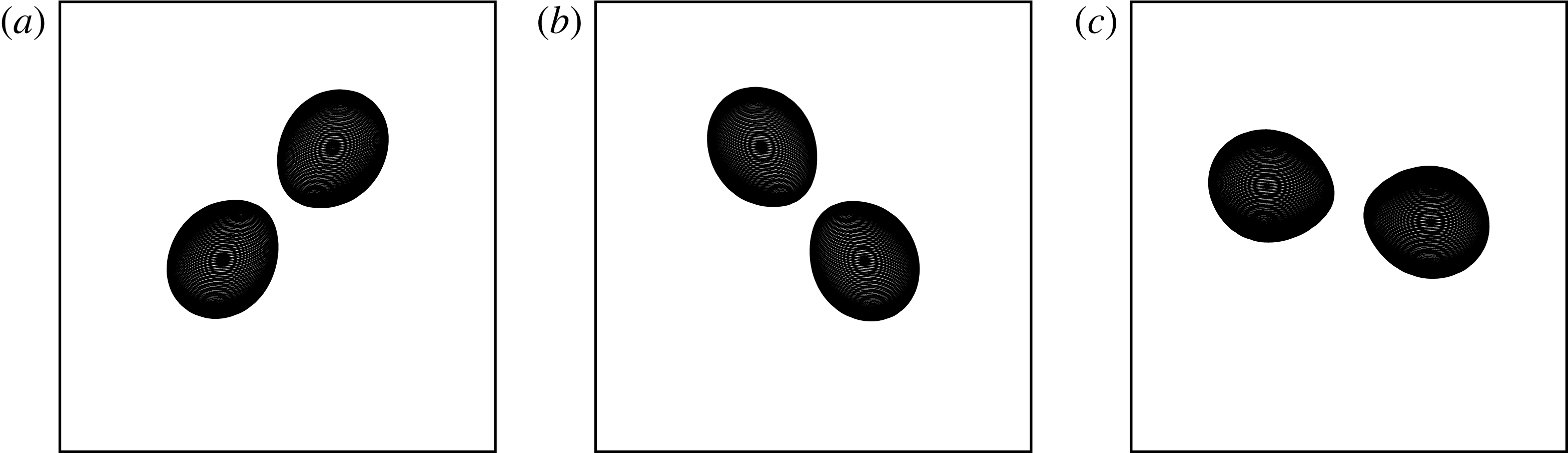
Figure 13. Evolution of the vortices, depicted by their bounding contours in each isopycnal, and in a reference frame stretched in the vertical direction by
 $N/f$
, for
$N/f$
, for
 $\unicode[STIX]{x1D6E5}_{v}=41/83$
,
$\unicode[STIX]{x1D6E5}_{v}=41/83$
,
 $Ro_{PV}=0.5$
and
$Ro_{PV}=0.5$
and
 $\unicode[STIX]{x1D6FF}/r_{m}=0.62$
. The view is orthographic at an angle of
$\unicode[STIX]{x1D6FF}/r_{m}=0.62$
. The view is orthographic at an angle of
 $60^{\circ }$
from the vertical. Times displayed are (a)
$60^{\circ }$
from the vertical. Times displayed are (a)
 $t_{QG}=31,~t=620$
, (b)
$t_{QG}=31,~t=620$
, (b)
 $t_{QG}=42,~t=840$
and (c)
$t_{QG}=42,~t=840$
and (c)
 $t_{QG}=50,~t=1000$
.
$t_{QG}=50,~t=1000$
.

Figure 14. Evolution of the vortices, depicted by their bounding contours in each isopycnal, and in a reference frame stretched in the vertical direction by
 $N/f$
, for
$N/f$
, for
 $\unicode[STIX]{x1D6E5}_{v}=41/83$
,
$\unicode[STIX]{x1D6E5}_{v}=41/83$
,
 $Ro_{PV}=-0.5$
and
$Ro_{PV}=-0.5$
and
 $\unicode[STIX]{x1D6FF}/r_{m}=0.62$
. The view is orthographic at an angle of
$\unicode[STIX]{x1D6FF}/r_{m}=0.62$
. The view is orthographic at an angle of
 $60^{\circ }$
from the vertical. Times displayed are (a)
$60^{\circ }$
from the vertical. Times displayed are (a)
 $t_{QG}=31,~t=620$
, (b)
$t_{QG}=31,~t=620$
, (b)
 $t_{QG}=42,~t=840$
and (c)
$t_{QG}=42,~t=840$
and (c)
 $t_{QG}=50,~t=1000$
.
$t_{QG}=50,~t=1000$
.
As mentioned in § 3, the shape of vortices influences their self-energy. The time evolution of the best-fit semi-axes lengths, normalised by their initial values, is shown in figure 5. Initially, the vortices have a unit mean height-to-width aspect ratio in stretched coordinates
 $(x,y,z^{\ast }=zN/f)$
where
$(x,y,z^{\ast }=zN/f)$
where
 $(a,b,c)$
are computed. Since the vortices are typically elongated along the axis joining their centroids (see figure 1), the lengths
$(a,b,c)$
are computed. Since the vortices are typically elongated along the axis joining their centroids (see figure 1), the lengths
 $a$
and
$a$
and
 $c$
are the horizontal semi-axis lengths while the intermediate length
$c$
are the horizontal semi-axis lengths while the intermediate length
 $b$
is a vertical semi-axis length at
$b$
is a vertical semi-axis length at
 $t=0$
. Figure 5 shows oscillations of
$t=0$
. Figure 5 shows oscillations of
 $a$
and
$a$
and
 $c$
, indicating a quasi-periodic pulsation of the vortices. Figures 6 and 7 illustrate the time evolution of the vortices for the two cases. The amplitude of these oscillations, a measure of the amplitude of the deformation of the vortices, is roughly of the same order of magnitude for cyclones and anticyclones when
$c$
, indicating a quasi-periodic pulsation of the vortices. Figures 6 and 7 illustrate the time evolution of the vortices for the two cases. The amplitude of these oscillations, a measure of the amplitude of the deformation of the vortices, is roughly of the same order of magnitude for cyclones and anticyclones when
 $\unicode[STIX]{x1D6E5}_{v}=0$
. Hence deformation plays a similar role in both cases. We can see, however, a much more pronounced increase of
$\unicode[STIX]{x1D6E5}_{v}=0$
. Hence deformation plays a similar role in both cases. We can see, however, a much more pronounced increase of
 $b/b_{0}$
for anticyclones than for cyclones. The increase is, in fact, associated with a tilt of the semi-axis, which began as vertical at
$b/b_{0}$
for anticyclones than for cyclones. The increase is, in fact, associated with a tilt of the semi-axis, which began as vertical at
 $t=0$
. This has been confirmed by analysing the eigenvector of
$t=0$
. This has been confirmed by analysing the eigenvector of
 ${\mathcal{B}}$
associated with the direction of the axis (results not shown). Hence, anticyclones appear to be vertically sheared. Since
${\mathcal{B}}$
associated with the direction of the axis (results not shown). Hence, anticyclones appear to be vertically sheared. Since
 $\unicode[STIX]{x1D6E5}_{v}=0$
, the initial configuration is symmetric with respect to the plane
$\unicode[STIX]{x1D6E5}_{v}=0$
, the initial configuration is symmetric with respect to the plane
 $z=0$
, and the shear is not imposed by the flow geometry. We conjecture that this tilt is the trace of a tilt instability which affects anticyclones predominantly. This may explain why anticyclones appear to deform more when an enhanced vertical shear, associated with
$z=0$
, and the shear is not imposed by the flow geometry. We conjecture that this tilt is the trace of a tilt instability which affects anticyclones predominantly. This may explain why anticyclones appear to deform more when an enhanced vertical shear, associated with
 $\unicode[STIX]{x1D6E5}_{v}>0$
, is present. This is discussed next.
$\unicode[STIX]{x1D6E5}_{v}>0$
, is present. This is discussed next.
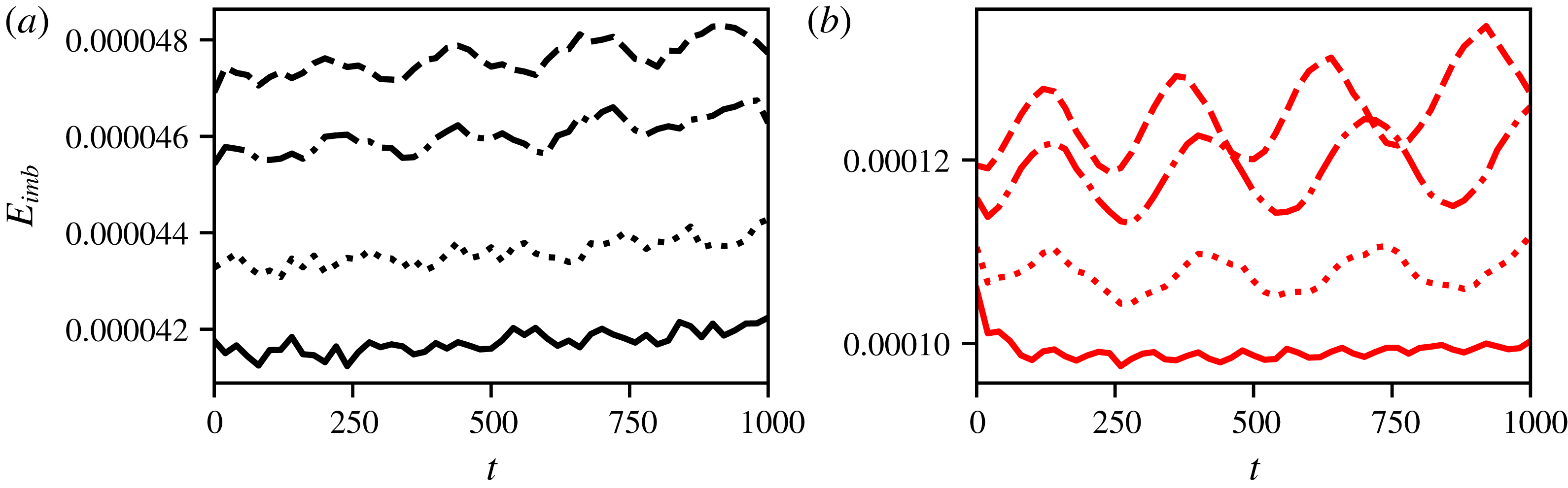
Figure 15. Evolution of the imbalanced energy
 $E_{imb}$
for
$E_{imb}$
for
 $Ro_{PV}=0.5$
(a) and
$Ro_{PV}=0.5$
(a) and
 $Ro_{PV}=-0.5$
(b). The simulations have resolution
$Ro_{PV}=-0.5$
(b). The simulations have resolution
 $256^{3}$
(set II) and correspond to
$256^{3}$
(set II) and correspond to
 $\unicode[STIX]{x1D6E5}_{v}=0,~\unicode[STIX]{x1D6FF}/r_{m}=0.5$
(solid),
$\unicode[STIX]{x1D6E5}_{v}=0,~\unicode[STIX]{x1D6FF}/r_{m}=0.5$
(solid),
 $\unicode[STIX]{x1D6E5}_{v}=11/83,~\unicode[STIX]{x1D6FF}/r_{m}=0.48$
(dotted),
$\unicode[STIX]{x1D6E5}_{v}=11/83,~\unicode[STIX]{x1D6FF}/r_{m}=0.48$
(dotted),
 $\unicode[STIX]{x1D6E5}_{v}=41/83,~\unicode[STIX]{x1D6FF}/r_{m}=0.62$
(dashed-dotted) and
$\unicode[STIX]{x1D6E5}_{v}=41/83,~\unicode[STIX]{x1D6FF}/r_{m}=0.62$
(dashed-dotted) and
 $\unicode[STIX]{x1D6E5}_{v}=62/83,~\unicode[STIX]{x1D6FF}/r_{m}=0.55$
(dashed).
$\unicode[STIX]{x1D6E5}_{v}=62/83,~\unicode[STIX]{x1D6FF}/r_{m}=0.55$
(dashed).
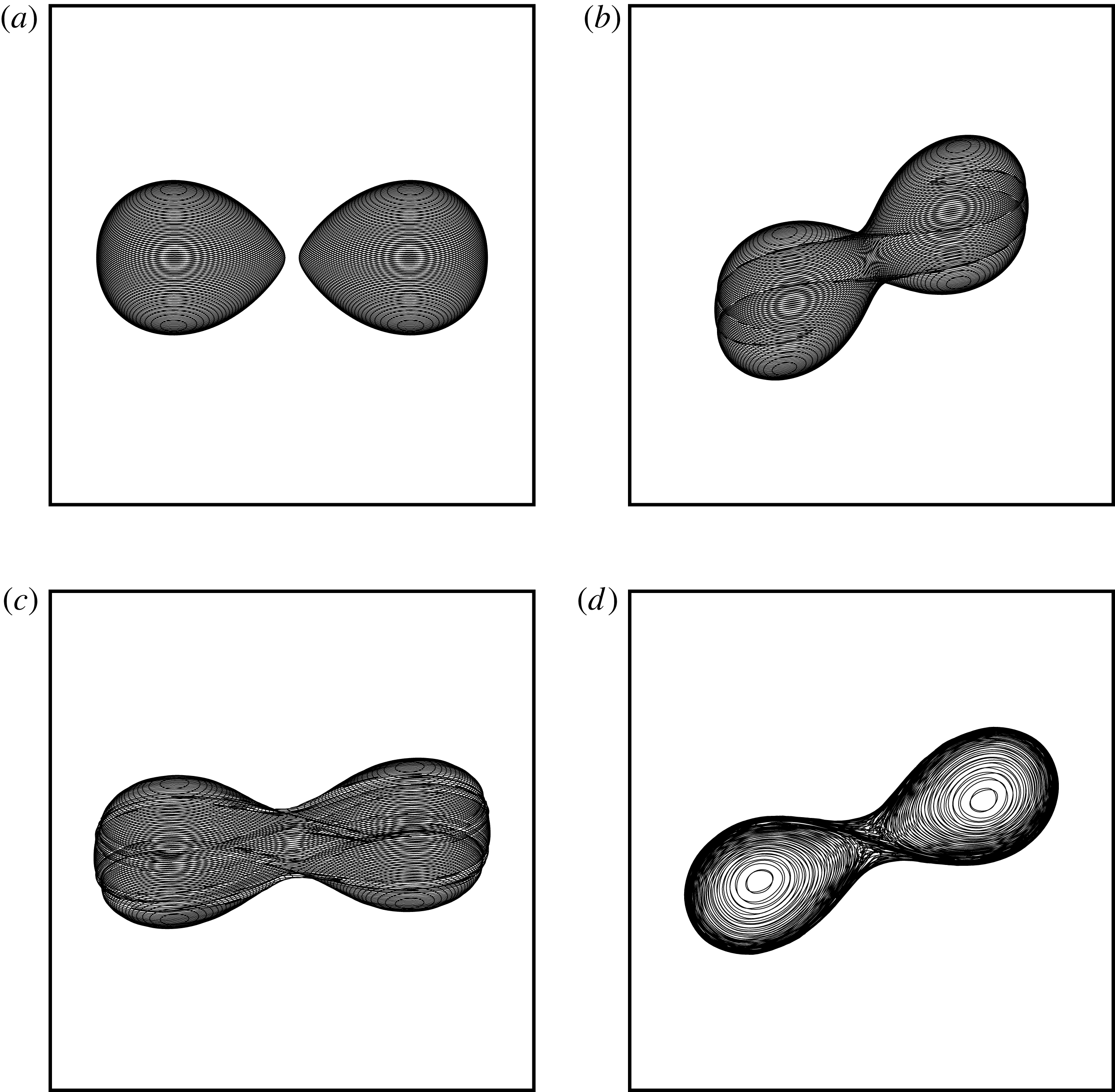
Figure 16. Evolution of the vortices, depicted by their bounding contours in each isopycnal, and in a reference frame stretched in the vertical direction by
 $N/f$
, for
$N/f$
, for
 $\unicode[STIX]{x1D6E5}_{v}=0$
,
$\unicode[STIX]{x1D6E5}_{v}=0$
,
 $Ro_{PV}=0.6$
and
$Ro_{PV}=0.6$
and
 $\unicode[STIX]{x1D6FF}/r_{m}=0.18$
. The view is orthographic at an angle of
$\unicode[STIX]{x1D6FF}/r_{m}=0.18$
. The view is orthographic at an angle of
 $60^{\circ }$
from the vertical in panels (a–c). Panel (d) provides a top view. Times displayed are (a)
$60^{\circ }$
from the vertical in panels (a–c). Panel (d) provides a top view. Times displayed are (a)
 $t_{QG}=t=0$
, (b)
$t_{QG}=t=0$
, (b)
 $t_{QG}=5,~t=83.3$
, (c)
$t_{QG}=5,~t=83.3$
, (c)
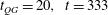 $t_{QG}=20,~t=333$
and (d)
$t_{QG}=20,~t=333$
and (d)
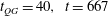 $t_{QG}=40,~t=667$
.
$t_{QG}=40,~t=667$
.

Figure 17. Evolution of the vortices for
 $\unicode[STIX]{x1D6E5}_{v}=0$
,
$\unicode[STIX]{x1D6E5}_{v}=0$
,
 $Ro_{PV}=-0.6$
and
$Ro_{PV}=-0.6$
and
 $\unicode[STIX]{x1D6FF}/r_{m}=0.18$
. The view is orthographic at an angle of
$\unicode[STIX]{x1D6FF}/r_{m}=0.18$
. The view is orthographic at an angle of
 $60^{\circ }$
from the vertical in panels (a–c). Panel (d) provides a top view. Times displayed are (a)
$60^{\circ }$
from the vertical in panels (a–c). Panel (d) provides a top view. Times displayed are (a)
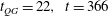 $t_{QG}=22,~t=366$
, (b)
$t_{QG}=22,~t=366$
, (b)
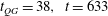 $t_{QG}=38,~t=633$
, (c)
$t_{QG}=38,~t=633$
, (c)
 $t_{QG}=45,~t=750$
and (d)
$t_{QG}=45,~t=750$
and (d)
 $t_{QG}=49,~t=817$
.
$t_{QG}=49,~t=817$
.

Figure 18. (a) Evolution of the distance
 $d$
between the vortex centroids for
$d$
between the vortex centroids for
 $Ro_{PV}=0.6$
(black) and
$Ro_{PV}=0.6$
(black) and
 $Ro_{PV}=-0.6$
(red) for
$Ro_{PV}=-0.6$
(red) for
 $\unicode[STIX]{x1D6E5}_{v}=0$
and
$\unicode[STIX]{x1D6E5}_{v}=0$
and
 $\unicode[STIX]{x1D6FF}/r_{m}=0.18$
. (b) Evolution of the best-fit ellipsoid. Black lines represent results for
$\unicode[STIX]{x1D6FF}/r_{m}=0.18$
. (b) Evolution of the best-fit ellipsoid. Black lines represent results for
 $Ro_{PV}=0.6$
, red lines for
$Ro_{PV}=0.6$
, red lines for
 $Ro_{PV}=-0.6$
. The quantities plotted are
$Ro_{PV}=-0.6$
. The quantities plotted are
 $a/a_{0}$
(solid),
$a/a_{0}$
(solid),
 $b/b_{0}$
(dotted) and
$b/b_{0}$
(dotted) and
 $c/c_{0}$
(dashed).
$c/c_{0}$
(dashed).
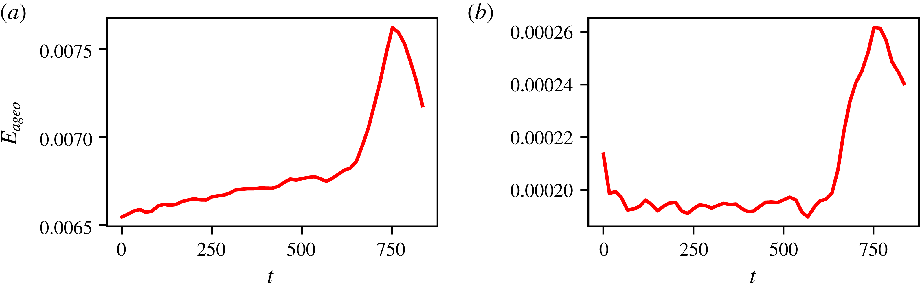
Figure 19. (a) Evolution of the ageostrophic energy
 $E_{ageo}$
for
$E_{ageo}$
for
 $Ro_{PV}=-0.6$
for
$Ro_{PV}=-0.6$
for
 $\unicode[STIX]{x1D6E5}_{v}=0$
and
$\unicode[STIX]{x1D6E5}_{v}=0$
and
 $\unicode[STIX]{x1D6FF}/r_{m}=0.18$
. (b) Evolution of the imbalanced energy
$\unicode[STIX]{x1D6FF}/r_{m}=0.18$
. (b) Evolution of the imbalanced energy
 $E_{imb}$
for the same simulation.
$E_{imb}$
for the same simulation.

Figure 20. Evolution of the vortices for
 $\unicode[STIX]{x1D6E5}_{v}=62/83$
,
$\unicode[STIX]{x1D6E5}_{v}=62/83$
,
 $Ro_{PV}=-0.5$
and
$Ro_{PV}=-0.5$
and
 $\unicode[STIX]{x1D6FF}/r_{m}=0.52$
. The view is orthographic at an angle of
$\unicode[STIX]{x1D6FF}/r_{m}=0.52$
. The view is orthographic at an angle of
 $60^{\circ }$
from the vertical. Times displayed are (a)
$60^{\circ }$
from the vertical. Times displayed are (a)
 $t_{QG}=t=0$
, (b)
$t_{QG}=t=0$
, (b)
 $t_{QG}=35,~t=700$
, (c)
$t_{QG}=35,~t=700$
, (c)
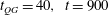 $t_{QG}=40,~t=900$
and (d)
$t_{QG}=40,~t=900$
and (d)
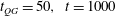 $t_{QG}=50,~t=1000$
.
$t_{QG}=50,~t=1000$
.
Figure 21. (a) Evolution of the best-fit ellipsoid semi-axis lengths for
 $\unicode[STIX]{x1D6E5}_{v}=62/83$
,
$\unicode[STIX]{x1D6E5}_{v}=62/83$
,
 $Ro_{PV}=-0.5$
and
$Ro_{PV}=-0.5$
and
 $\unicode[STIX]{x1D6FF}/r_{m}=0.52$
. (b) Evolution of the ageostrophic energy
$\unicode[STIX]{x1D6FF}/r_{m}=0.52$
. (b) Evolution of the ageostrophic energy
 $E_{ageo}$
versus
$E_{ageo}$
versus
 $t$
, and (c) evolution of the imbalance energy
$t$
, and (c) evolution of the imbalance energy
 $E_{imb}$
versus
$E_{imb}$
versus
 $t$
for the same simulation.
$t$
for the same simulation.
We now turn to the influence of the vertical offset
 $\unicode[STIX]{x1D6E5}_{v}$
. We further analyse three cases, with
$\unicode[STIX]{x1D6E5}_{v}$
. We further analyse three cases, with
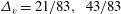 $\unicode[STIX]{x1D6E5}_{v}=21/83,~43/83$
and
$\unicode[STIX]{x1D6E5}_{v}=21/83,~43/83$
and
 $62/83$
. All these cases are run at a grid resolution
$62/83$
. All these cases are run at a grid resolution
 $n_{g}^{3}=256^{3}$
. For each case we consider
$n_{g}^{3}=256^{3}$
. For each case we consider
 $Ro_{PV}=\pm 0.5$
. As above, figures 8–10 show the time evolution of the ageostrophic energy, of the horizontal distance
$Ro_{PV}=\pm 0.5$
. As above, figures 8–10 show the time evolution of the ageostrophic energy, of the horizontal distance
 $d$
between the vortex centroids, and of the vortex semi-axis lengths. The evolution of the vortices for the first four cases is presented in figure 11 for
$d$
between the vortex centroids, and of the vortex semi-axis lengths. The evolution of the vortices for the first four cases is presented in figure 11 for
 $Ro_{PV}=0.5$
and
$Ro_{PV}=0.5$
and
 $\unicode[STIX]{x1D6E5}_{v}=21/83$
, in figure 12 for
$\unicode[STIX]{x1D6E5}_{v}=21/83$
, in figure 12 for
 $Ro_{PV}=-0.5$
and
$Ro_{PV}=-0.5$
and
 $\unicode[STIX]{x1D6E5}_{v}=21/83$
, in figure 13 for
$\unicode[STIX]{x1D6E5}_{v}=21/83$
, in figure 13 for
 $Ro_{PV}=0.5$
and
$Ro_{PV}=0.5$
and
 $\unicode[STIX]{x1D6E5}_{v}=41/83$
, and in figure 14 for
$\unicode[STIX]{x1D6E5}_{v}=41/83$
, and in figure 14 for
 $Ro_{PV}=-0.5$
and
$Ro_{PV}=-0.5$
and
 $\unicode[STIX]{x1D6E5}_{v}=41/83$
. The general trend where cyclones move closer together and anticyclones move apart persists when
$\unicode[STIX]{x1D6E5}_{v}=41/83$
. The general trend where cyclones move closer together and anticyclones move apart persists when
 $\unicode[STIX]{x1D6E5}_{v}>0$
and is therefore a generic feature of the interaction. We notice, however, that this main drift is subject to oscillations of large amplitude. These oscillations are also noticeable in the time evolution of the ageostrophic energy. Again, the time evolution of
$\unicode[STIX]{x1D6E5}_{v}>0$
and is therefore a generic feature of the interaction. We notice, however, that this main drift is subject to oscillations of large amplitude. These oscillations are also noticeable in the time evolution of the ageostrophic energy. Again, the time evolution of
 $E_{ageop}$
is consistent with the time evolution of the vortex separation distance
$E_{ageop}$
is consistent with the time evolution of the vortex separation distance
 $d$
, and follows the pattern previously observed for
$d$
, and follows the pattern previously observed for
 $\unicode[STIX]{x1D6E5}_{v}=0$
. The main difference from the aligned cases with
$\unicode[STIX]{x1D6E5}_{v}=0$
. The main difference from the aligned cases with
 $\unicode[STIX]{x1D6E5}_{v}=0$
is found in the amplitude of the oscillations. This is particularly evident in the time evolution of
$\unicode[STIX]{x1D6E5}_{v}=0$
is found in the amplitude of the oscillations. This is particularly evident in the time evolution of
 $a(t)$
,
$a(t)$
,
 $b(t)$
and
$b(t)$
and
 $c(t)$
. Contrary to the cases with
$c(t)$
. Contrary to the cases with
 $\unicode[STIX]{x1D6E5}_{v}=0$
, there is a large difference in the amplitude of the oscillations for cyclones and anticyclones, with the latter exhibiting significantly higher amplitudes. We associate this difference to the greater sensitivity of the anticyclones to vertical shear. The greater deformation means that anticyclones may touch and merge even if overall the individual vortex centroids tend to move away from each other. As a consequence, anticyclones are able to merge from further apart compared to cyclones for larger vertical offsets.
$\unicode[STIX]{x1D6E5}_{v}=0$
, there is a large difference in the amplitude of the oscillations for cyclones and anticyclones, with the latter exhibiting significantly higher amplitudes. We associate this difference to the greater sensitivity of the anticyclones to vertical shear. The greater deformation means that anticyclones may touch and merge even if overall the individual vortex centroids tend to move away from each other. As a consequence, anticyclones are able to merge from further apart compared to cyclones for larger vertical offsets.
Finally, figure 15 illustrates the time evolution of the imbalanced energy,
 $E_{imb}$
, for the eight cases discussed above. (This is computed using
$E_{imb}$
, for the eight cases discussed above. (This is computed using
 $\unicode[STIX]{x1D753}\prime =\unicode[STIX]{x1D753}_{imb}$
in (4.5).) If we disregard the very early phase of the time evolution, which is affected by the artificial initial PV ramping, the overall trend is a very small increase in
$\unicode[STIX]{x1D753}\prime =\unicode[STIX]{x1D753}_{imb}$
in (4.5).) If we disregard the very early phase of the time evolution, which is affected by the artificial initial PV ramping, the overall trend is a very small increase in
 $E_{imb}$
with time, with oscillations corresponding to the vortex shape variations discussed above. The imbalanced energies
$E_{imb}$
with time, with oscillations corresponding to the vortex shape variations discussed above. The imbalanced energies
 $E_{imb}$
of cyclones and anticyclones having the same
$E_{imb}$
of cyclones and anticyclones having the same
 $|Ro_{PV}|$
are compared in figure 15. Anticyclones produce significantly larger levels of imbalanced energy, consistent with the fact that anticyclones are more intense and more readily deform. The deformation of the vortices in particular is likely to enhance the spontaneous generation of IGWs. (Circular vortices exist which do not radiate.)
$|Ro_{PV}|$
are compared in figure 15. Anticyclones produce significantly larger levels of imbalanced energy, consistent with the fact that anticyclones are more intense and more readily deform. The deformation of the vortices in particular is likely to enhance the spontaneous generation of IGWs. (Circular vortices exist which do not radiate.)
We next present two cases of interaction leading to merger for
 $\unicode[STIX]{x1D6E5}_{v}=0$
, using results obtained at
$\unicode[STIX]{x1D6E5}_{v}=0$
, using results obtained at
 $n_{g}^{3}=256^{3}$
. We choose a gap
$n_{g}^{3}=256^{3}$
. We choose a gap
 $\unicode[STIX]{x1D6FF}/r_{m}=0.18$
which is smaller than the critical merging gap for both cyclones at
$\unicode[STIX]{x1D6FF}/r_{m}=0.18$
which is smaller than the critical merging gap for both cyclones at
 $Ro_{PV}=0.6$
and anticyclones at
$Ro_{PV}=0.6$
and anticyclones at
 $Ro_{PV}=-0.6$
. Recall that, for
$Ro_{PV}=-0.6$
. Recall that, for
 $\unicode[STIX]{x1D6E5}_{v}=0$
, cyclones are able to merge from further apart than anticyclones. Figure 16 illustrates the flow evolution by displaying the PV contours defining the vortex boundaries at four times. The two vortices merge by
$\unicode[STIX]{x1D6E5}_{v}=0$
, cyclones are able to merge from further apart than anticyclones. Figure 16 illustrates the flow evolution by displaying the PV contours defining the vortex boundaries at four times. The two vortices merge by
 $t=50$
(
$t=50$
(
 $t_{QG}=3$
) and form a dumbbell vortex where the two main volumes of PV are linked by a bridge. The structure is metastable and persists in time. The merged vortex is strikingly similar to those obtained in the QG model (Reinaud & Dritschel Reference Reinaud and Dritschel2002), indicating that the leading-order behaviour is consistent with the underlying near-balanced conditions.
$t_{QG}=3$
) and form a dumbbell vortex where the two main volumes of PV are linked by a bridge. The structure is metastable and persists in time. The merged vortex is strikingly similar to those obtained in the QG model (Reinaud & Dritschel Reference Reinaud and Dritschel2002), indicating that the leading-order behaviour is consistent with the underlying near-balanced conditions.
Figure 17 shows a similar interaction for anticyclones. Again, the vortices merge but later than the cyclones do. The vortices touch by
 $t=633$
(
$t=633$
(
 $t_{QG}=38$
), and by
$t_{QG}=38$
), and by
 $t=750$
(
$t=750$
(
 $t_{QG}=45$
) the merged vortex has fully formed. The shape of the dumbbell vortex is, however, different. The outer edges of the cyclonic dumbbell are concave while the outer edges of the anticyclonic one are convex. This indicates that more PV has moved towards the centre for the anticyclone, making it more compact. Conservation of the angular impulse dictates that some PV must move away from the centre to compensate. This explains why peripheral PV filaments near the bottom and top outer edges of the structure move away from the centre for anticyclones.
$t_{QG}=45$
) the merged vortex has fully formed. The shape of the dumbbell vortex is, however, different. The outer edges of the cyclonic dumbbell are concave while the outer edges of the anticyclonic one are convex. This indicates that more PV has moved towards the centre for the anticyclone, making it more compact. Conservation of the angular impulse dictates that some PV must move away from the centre to compensate. This explains why peripheral PV filaments near the bottom and top outer edges of the structure move away from the centre for anticyclones.
Many of the trends analysed previously recur in these merging situations. For example, figure 18 shows that cyclones drift towards each other then merge rapidly. On the other hand, anticyclones drift away from each other, delaying merger. The time evolution of the semi-axes lengths of the best-fit ellipsoid marks clearly the time of merger by the sudden increase of
 $c$
, the largest length corresponding to the maximum horizontal span of the largest vortex identified. For anticyclones, the merger is accompanied by a peak of ageostrophic and imbalanced energies, as shown in figure 19. The merger is a violent event and a source of IGW generation and enhanced ageostrophic motion. Similar peaks are less pronounced for cyclones. This is related to the fact that cyclones have smaller relative vorticity and buoyancy anomalies compared to anticyclones.
$c$
, the largest length corresponding to the maximum horizontal span of the largest vortex identified. For anticyclones, the merger is accompanied by a peak of ageostrophic and imbalanced energies, as shown in figure 19. The merger is a violent event and a source of IGW generation and enhanced ageostrophic motion. Similar peaks are less pronounced for cyclones. This is related to the fact that cyclones have smaller relative vorticity and buoyancy anomalies compared to anticyclones.
We finally illustrate the merger of vertically offset anticyclones which are able to merge from large initial separation distances. We consider a case with
 $\unicode[STIX]{x1D6E5}_{v}=62/83$
,
$\unicode[STIX]{x1D6E5}_{v}=62/83$
,
 $\unicode[STIX]{x1D6FF}/r_{m}=0.52$
and
$\unicode[STIX]{x1D6FF}/r_{m}=0.52$
and
 $Ro_{PV}=-0.5$
at resolution
$Ro_{PV}=-0.5$
at resolution
 $n_{g}^{3}=256^{3}$
. As seen in figure 20(a), the vortices are initially well separated. Then the vortices start to shed a small amount of filamentary PV at
$n_{g}^{3}=256^{3}$
. As seen in figure 20(a), the vortices are initially well separated. Then the vortices start to shed a small amount of filamentary PV at
 $t=460$
(
$t=460$
(
 $t_{QG}=23$
). This occurs before the vortices merge. This means that these debris are not the result of the merger but rather the trace of an instability which affects each vortex. This is consistent with our conjecture that these vortices, in particular anticyclones, are sensitive to a mode of instability for which vertical shear is important. The shedding of filaments continues until
$t_{QG}=23$
). This occurs before the vortices merge. This means that these debris are not the result of the merger but rather the trace of an instability which affects each vortex. This is consistent with our conjecture that these vortices, in particular anticyclones, are sensitive to a mode of instability for which vertical shear is important. The shedding of filaments continues until
 $t=780$
(
$t=780$
(
 $t_{QG}=38$
) when the two main vortices finally merge. The resulting vortex is a tilted dumbbell vortex surrounded by a ring of filamentary PV (see figure 20
d).
$t_{QG}=38$
) when the two main vortices finally merge. The resulting vortex is a tilted dumbbell vortex surrounded by a ring of filamentary PV (see figure 20
d).
Figure 21 shows the deformation of the largest vortex, as well as the evolution of both
 $E_{ageo}$
and
$E_{ageo}$
and
 $E_{imb}$
. As before, the sudden increase of
$E_{imb}$
. As before, the sudden increase of
 $c$
, the largest semi-axis length representative of the largest dimension of the vortex, indicates the onset of merger. The merger process is also accompanied by a steep increase in
$c$
, the largest semi-axis length representative of the largest dimension of the vortex, indicates the onset of merger. The merger process is also accompanied by a steep increase in
 $E_{ageo}$
and
$E_{ageo}$
and
 $E_{imb}$
as observed before. We also notice a secondary peak of
$E_{imb}$
as observed before. We also notice a secondary peak of
 $E_{ageo}$
and
$E_{ageo}$
and
 $E_{imb}$
, around
$E_{imb}$
, around
 $t=430$
, corresponding to the filamentation of the vortices. Hence filamentation occurs during a phase of strong ageostrophic activity.
$t=430$
, corresponding to the filamentation of the vortices. Hence filamentation occurs during a phase of strong ageostrophic activity.
5 Conclusions
In this paper, we have studied the merger of two finite Rossby and finite Froude number vortices. Such vortices are representative of the submesoscale eddies that are omnipresent in the oceans. Owing to the large number of submesoscale eddies observed in the oceans, close-range interactions between vortices are likely. We have shown that the interaction critically depends on both the Rossby number and the vertical offset of the vortices. Horizontally aligned cyclones are able to merge from further apart than anticyclones. Cyclones tend to move closer together while anticyclones tend to move further apart.
On the other hand, anticyclones appear to be more sensitive to vertical shear, and deform more readily than cyclones. When the vertical shear is enhanced by a vertical offset between the vortices, the increase in deformation can trigger the merger of anticyclones from further initial separation distances. The influence of vertical shear on a single cyclone or anticyclone should be addressed in future research; our results suggest that anticyclones may be unstable to a shear or tilt mode.
A possible extension of the work is the addition of opposite-signed PV above and below the structure as observed in Meddies (Mediterranean Water eddies), as well as studying the vertical alignment of like-signed structures lying at different depths.
Submesoscale vortices can often, but not always, be generated by the unstable interaction of a current with coasts or bathymetry (bottom topography). Another natural extension of the research is to consider the effect of a coastline and/or of a sloping seabed on the interaction. This will be the focus of future research.
Acknowledgements
Partial support for this research has come from the UK Engineering and Physical Sciences Research Council (grant number EP/H001794/1).


