


1. Introduction
When small, rigid particles are immersed in a fluid, material (e.g. a solute) may be transferred away from the surface by convection and diffusion. We shall refer to this process as mass transfer, although an analogous problem exists for heat transfer. The engineered and natural worlds are replete with examples: planktonic osmotrophs absorb dissolved nutrients (Karp-Boss, Boss & Jumars Reference Karp-Boss, Boss and Jumars1996; Pahlow, Riebesell & Wolf-Gladrow Reference Pahlow, Riebesell and Wolf-Gladrow1997; Guasto, Rusconi & Stocker Reference Guasto, Rusconi and Stocker2012), bacterial hosts encounter viruses (Guasto et al. Reference Guasto, Rusconi and Stocker2012), crystals are grown in agitated suspension to produce pharmaceuticals and industrial products (Myerson Reference Myerson2002) and microplastics leach and sorb pollutants in ocean waters (Suhrhoff & Scholz-Böttcher Reference Suhrhoff and Scholz-Böttcher2016; Law Reference Law2017; Seidensticker et al. Reference Seidensticker, Zarfl, Cirpka, Fellenberg and Grathwohl2017). The examples cited above have in common that the solid particle exchanging material is rarely ever spherical, is usually small compared to the flow features in which it is embedded and the material diffuses slowly such that convection is the dominant mechanism of mass transfer. The question then naturally follows: What is the rate of mass transfer from the surface?
This question belongs to a general set of classical problems which have been well studied (see e.g. works summarised by Clift, Grace & Weber Reference Clift, Grace and Weber1978; Michaelides Reference Michaelides2003; Leal Reference Leal2012). The answer depends upon the competing effects of convection and diffusion, as parametrised by the Péclet number,  ${Pe}$. When ${Pe} \ll 1$, conduction dominates inside an inner region near the particle and the effects of shape are readily accounted for (Batchelor Reference Batchelor1979; Acrivos Reference Acrivos1980; Feng & Michaelides Reference Feng and Michaelides1997; Pozrikidis Reference Pozrikidis1997). When ${Pe} \gg 1$, convection dominates the mass transfer process and the surface flux of solute is determined by the particle geometry and the nature of the relative flow field, parametrised by the Reynolds number, $Re$. In closed-streamline flows, the solute simply recirculates around the particle and the surface flux approaches a constant as ${Pe} \rightarrow \infty$ (Frankel & Acrivos Reference Frankel and Acrivos1968; Poe & Acrivos Reference Poe and Acrivos1976). When the particle is surrounded by a region of open streamlines (or pathlines), the solution to the convection–diffusion problem takes the form of a thin concentration boundary layer around the particle. For this case, Acrivos (Reference Acrivos1960) and later Acrivos & Goddard (Reference Acrivos and Goddard1965) introduced asymptotic methods to compute the mass transfer rate, which scales as ${Pe}^{1/3}$. The flow and the geometry of the problem then determine the scaling coefficient, which prescribes the surface flux.
For sufficiently small particles,  $Re \ll 1$ and the surrounding relative flow field may be well approximated by a Stokes flow consisting of a background uniform flow or linear shear, plus a perturbation owing to the presence of the particle. The available analytical results in the high Péclet number, low Reynolds number regime are generally limited to simplified flows or geometries. A general solution to this problem would have great utility, because solid particles are often neither spherical nor subject to motions as simple as uniform or axisymmetric flows (Leal Reference Leal2012). Specific analytical results are available for spheres in uniform flow (Acrivos Reference Acrivos1960; Acrivos & Taylor Reference Acrivos and Taylor1962) or arbitrary linear shear (Gupalo & Riazantsev Reference Gupalo and Riazantsev1972; Poe & Acrivos Reference Poe and Acrivos1976; Batchelor Reference Batchelor1979) and axisymmetric bodies in uniform flow (Sehlin Reference Sehlin1969; Gupalo, Polianin & Riazantsev Reference Gupalo, Polianin and Riazantsev1976; Leal Reference Leal2012; Dehdashti & Masoud Reference Dehdashti and Masoud2020). To our knowledge, equivalent results are not available for arbitrary bodies with high Péclet numbers in an arbitrary linear shear. Experimental and numerical studies have focused on the uniform flow case typically with ${Pe} = O(Re )$ (Masliyah & Epstein Reference Masliyah and Epstein1972; Clift et al. Reference Clift, Grace and Weber1978; Sparrow, Abraham & Tong Reference Sparrow, Abraham and Tong2004; Kishore & Gu Reference Kishore and Gu2011; Ke et al. Reference Ke, Shu, Zhang, Yuan and Yang2018; Ma & Zhao Reference Ma and Zhao2020); relatively few studies have examined the high Péclet number, low Reynolds number regime numerically (Karp-Boss et al. Reference Karp-Boss, Boss and Jumars1996; Pahlow et al. Reference Pahlow, Riebesell and Wolf-Gladrow1997) and the results available for linear shear flows are limited to a handful of cases. Therefore, additional empirical data are needed for the general case of arbitrary linear shear to support a generalisation of asymptotic results.
For freely suspended particles, an additional complication arises which affects the mass transfer rate. In the absence of body forces, such as the case of neutrally buoyant particles, the drag and consequently the slip velocity vanish, such that convection is provided by the linear shear alone. However, the fluid may exert a couple upon the particle (Jeffery Reference Jeffery1922), which in the absence of a restoring torque will result in the steady precession or rotation of the particle about its axis. As a result, the flow field around the particle and resultant surface flux is in general unsteady (Pahlow et al. Reference Pahlow, Riebesell and Wolf-Gladrow1997). However, for spherical particles, Batchelor (Reference Batchelor1979) and Batchelor (Reference Batchelor1980) argued that the unsteady contribution to the scalar flux may be neglected at large Péclet number, so that the average flow field perceived by the body determines the average mass transfer rate.
In this article, we extend the work of Acrivos & Goddard (Reference Acrivos and Goddard1965) and Batchelor (Reference Batchelor1979) to consider the mass transfer rate due to convection and diffusion from an arbitrary body in an unsteady, open pathline flow at high Péclet number. We then apply this analysis to determine the mass transfer rate from a neutrally buoyant spheroid freely suspended in an arbitrary linear shear. We obtain asymptotic expressions for the transfer rate in the resultant average flow field and compare these to the results of numerical simulations, which provide a quantitative test of the accuracy of the asymptotic approximation. Our results allow us to examine the role of particle shape in the mass transfer process for a very broad class of flows and open up new possibilities in the numerical simulation of mass transfer in particle suspensions.
The paper is structured as follows. In § 2, we review the theoretical background of the problem and derive a general form for the mass transfer coefficient for an arbitrary particle in an unsteady, time periodic flow. In § 3, we apply this general expression to the case of a freely suspended spheroid in Stokes flow. In § 4, we introduce a numerical test of the results given in § 3 and discuss the influence of particle shape upon the surface flux. We present a summary of our results and future perspectives in § 5.
2. The steady flux at large Péclet number
In this section, we shall extend the analyses of Acrivos & Goddard (Reference Acrivos and Goddard1965) and Batchelor (Reference Batchelor1979) to derive a general expression for the average solute flux from the surface of a particle of arbitrary shape in a steady, open-streamline flow. We begin by introducing the governing equations in dimensionless form, then examine the case of steady flow. Finally, we generalise the result to unsteady flow.
2.1. Governing equations
The mass transport from the surface of the particle is governed by the convection–diffusion equation. This may be written in dimensionless form as
 \begin{equation} \frac{\partial \theta}{\partial t} + \boldsymbol{u}\boldsymbol{\cdot}\boldsymbol{\nabla} \theta = \frac{1}{{Pe}}\nabla^2 \theta, \end{equation}
where  $\boldsymbol {u}(\boldsymbol {x},t)$ is the velocity field and $\theta (\boldsymbol {x},t)$ is the concentration of the solute (Leal Reference Leal2012). The characteristic length scale is $r$, the linear dimension of the particle, so that the spatial coordinate is non-dimensionalised as $\boldsymbol {x} = \boldsymbol {x}^*/r$. The characteristic time scale is prescribed by the shear rate $E^*$, so that time is non-dimensionalised as $t=t^*E^*$. The Péclet number is defined ${Pe} \equiv r^2 E^* / \kappa$, where $\kappa$ is the diffusion coefficient of the solute. Our convention is to write dimensional quantities with a superscript $^*$ unless otherwise stated.
We shall adopt a frame of reference moving with the particle, such that the boundary of the particle  $S_p$ is stationary. We impose the boundary condition
 \begin{equation} \left.\begin{array}{c@{}} \theta = 1 \quad \text{and}\quad \boldsymbol{u} = 0 \quad \text{for } \boldsymbol{x} \in S_p \\ \theta \rightarrow 0 \quad \text{as } |\boldsymbol{x}| \rightarrow \infty \end{array},\right\} \end{equation}
so that the concentration of solute at the particle surface is uniform. This boundary condition corresponds to non-dimensionalising the concentration field  $C(\boldsymbol {x}^*,t^*)$ as $\theta = (C-C_0)/(C_1-C_0)$, where $C_1$ and $C_0$ are the concentration of solute at the surface and infinity in physical units.
The non-dimensional measure of the surface flux  $Q$ is the Sherwood number
 \begin{equation} {Sh} = \frac{Q}{4{\rm \pi} r\kappa(C_1 - C_0)} ={-}\frac{1}{4{\rm \pi}} \iint_{S_p} \boldsymbol{\nabla} \theta \boldsymbol{\cdot} \mathrm{d}\boldsymbol{S}. \end{equation}
The denominator in (2.3) corresponds to the steady state flux from a sphere of radius  $r$ in the absence of flow. A convenient choice for the length scale $r$ is $\sqrt {A/4{\rm \pi} }$, where $A$ is the surface area of the particle. The Sherwood number is therefore the factor by which convection enhances the mass transfer relative to the diffusive flux from a spherical particle with the same surface area.
2.2. General solution of the surface flux in steady flow
In steady flow, the scalar transport equation reduces to
 \begin{equation} \boldsymbol{u}\boldsymbol{\cdot} \boldsymbol{\nabla} \theta = \frac{1}{{Pe}} \nabla^2 \theta. \end{equation}
We seek an asymptotic solution for (2.4) subject to (2.2) at large Péclet number.
At large Péclet number, the concentration of solute is small almost everywhere far from the particle, apart from a thin wake, along which material from the surface is swept. Near the particle, there is a concentration boundary layer whose thickness is  $O(\delta )$, across which there is a sharp jump in concentration. For the boundary layer approximation to hold, the pathlines near the surface of the particle must originate and terminate at infinity, such that the surface of the particle is exposed to a constant stream of fresh fluid. Recirculating regions (closed pathlines), which can occur in some geometries, are not permitted.
We shall construct a general curvilinear coordinate system  $(\xi , \eta , \zeta )$ to describe the flow near the surface in terms of the distance from the surface and the direction of the flow near the surface. This coordinate system is not necessarily orthogonal and we will find it useful to describe it in terms of the covariant coordinate vectors
 \begin{equation} \boldsymbol{h}_\xi = \frac{\partial \boldsymbol{x}}{\partial \xi}, \quad \boldsymbol{h}_\eta = \frac{\partial \boldsymbol{x}}{\partial \eta}, \quad \boldsymbol{h}_\zeta= \frac{\partial \boldsymbol{x}}{\partial \zeta}, \end{equation}
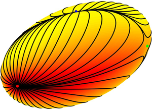
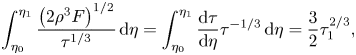
and their pathlines, which we have illustrated in figure 1. We note that the adoption of a general curvilinear coordinate system, rather than an orthogonal one, is crucial in the generalisation to an arbitrary flow or body.

Figure 1. Illustration of the curvilinear coordinate system  $(\xi ,\eta ,\zeta )$ defined on the surface ( $\xi =0$) of a spheroid in an arbitrary linear shear. Thick black lines show $\eta$-coordinate pathlines ( $\xi =0,\zeta =\text {const.}$), which are tangent to the local viscous shear stress on the surface. Thin grey lines are $\zeta$-coordinate pathlines ( $\xi = 0, \eta =\text {const.}$). Three fixed points of the surface streamlines are shown: red (source), green (saddle) and blue (sink).
The coordinate  $\xi$ is defined as the normal distance from the particle surface, so that at the particle surface, $\boldsymbol {h}_\xi$ is a unit vector normal to the surface. The $\eta$ and $\zeta$ coordinates lie tangent to the surface. We shall define the $\eta$ coordinate so that at a small distance $\xi$ above the surface, the component of fluid velocity which is tangent to the surface is parallel to $\boldsymbol {h}_\eta$. The curves along the $\eta$ direction are therefore ‘surface streamlines’ which are tangent to the direction of the surface velocity gradient $\boldsymbol {w} = \partial \boldsymbol {u}/\partial \xi |_{\xi =0}$.
We can therefore express the velocity near the surface as
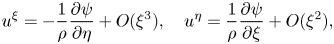
 \begin{align} \boldsymbol{u}&= u^\xi \boldsymbol{h}_\xi + u^\eta\boldsymbol{h}_\eta + u^\zeta\boldsymbol{h}_\zeta \nonumber\\ &= \boldsymbol{w}\xi + O(\xi^2), \end{align}
so that near the particle surface, the velocity components are of the form
 \begin{equation} u^\xi = G(\eta,\zeta)\xi^2 + O(\xi^3), \quad u^\eta = \xi F(\eta,\zeta) + O(\xi^2), \quad u^\zeta = O(\xi^2). \end{equation}
By definition, the velocity at the surface is zero; the tangential component  $u^\eta$ is linear in $\xi$ to leading order, whereas the surface-normal component is quadratic (Leal Reference Leal2012). The function $F(\eta , \zeta )$ is therefore obtained in terms of the velocity gradient at the surface of the particle as
 \begin{equation} F = \boldsymbol{w} \boldsymbol{\cdot} \boldsymbol{\nabla} \eta, \end{equation}
and is related to  $G(\eta ,\zeta )$ through the continuity equation.
To obtain the surface-normal velocity component  $u^\xi$, we express the continuity equation as (Grinfeld Reference Grinfeld2013)
 \begin{equation} \rho\nabla_i u^i = \frac{\partial (\rho u^\xi)}{\partial \xi} + \frac{\partial (\rho u^\eta)}{\partial \eta} + \frac{\partial (\rho u^\zeta)}{\partial \zeta} = 0, \end{equation}
where  $\rho = \rho (\eta , \zeta ) \equiv \sqrt {\det {g}}$ and $\det {g}$ is the determinant of the metric tensor ${\mathsf{g}}_{ij} \equiv \boldsymbol {h}_i\boldsymbol {\cdot }\boldsymbol {h}_j$. Since $g_{\xi \xi } = 1$, $g_{\xi \eta } = g_{\xi \zeta } = 0$ by definition, the physical interpretation of $\rho$ is a local area density of the surface streamlines, such that $\delta A = \rho \delta \eta \delta \zeta$ is the area covered by a small region on the surface measuring $\delta \eta$ along a surface streamline and $\delta \zeta$ across adjacent streamlines. We can then define a streamfunction $\psi$ as
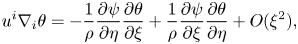
 \begin{equation} u^\xi ={-}\frac{1}{\rho} \frac{\partial \psi}{\partial \eta} + O(\xi^3), \quad u^\eta = \frac{1}{\rho} \frac{\partial \psi}{\partial \xi}+ O(\xi^2), \end{equation}
so that
 \begin{equation} \psi = \tfrac{1}{2}\xi^2 \rho F, \end{equation}
is a solution which satisfies (2.7a–c) and the continuity equation (2.9) to leading order in  $\xi$.
Writing (2.4) in these curvilinear coordinates, our solution now proceeds analogously to the works of Acrivos & Goddard (Reference Acrivos and Goddard1965) and Batchelor (Reference Batchelor1979). We shall formalise Batchelor's analysis here in our new curvilinear coordinate system for the purpose of exposition. To leading order in  $\xi$, the convection term is
 \begin{equation} u^i \nabla_i \theta ={-}\frac{1}{\rho}\frac{\partial \psi}{\partial \eta}\frac{\partial \theta}{\partial \xi} +\frac{1}{\rho}\frac{\partial \psi}{\partial \xi}\frac{\partial \theta}{\partial \eta} + O(\xi^2), \end{equation}
whereas the diffusion term may be written
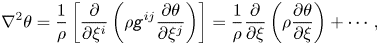 \begin{equation} \nabla^2 \theta = \frac{1}{\rho} \left[ \frac{\partial}{\partial \xi^i}\left(\rho {\mathsf{g}}^{ij} \frac{\partial \theta}{\partial \xi^j}\right) \right] = \frac{1}{\rho} \frac{\partial}{\partial \xi}\left(\rho \frac{\partial \theta}{\partial \xi}\right) + \cdots , \end{equation}
where  ${\mathsf{g}}^{ij}$ is the inverse metric tensor and $\xi ^i$ indexes the coordinates $(\xi ,\eta ,\zeta )$. The terms omitted in the expansion of (2.13) do not involve any gradients in $\xi$. By neglecting them, we assume that the diffusive flux of material across the surface is small in comparison to that normal to the surface. This essentially requires that the particle surface be smooth and contain no regions of extreme curvature where this assumption may break down.
We now rescale our coordinate system and streamfunction so that the surface-normal concentration gradient is  $O(1)$. Rescaling $\xi$ by the boundary layer thickness $\delta$, we write
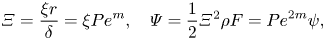 \begin{equation} \varXi = \frac{\xi r}{\delta} = \xi{Pe}^m, \quad \varPsi = \frac{1}{2}\varXi^2 \rho F = {Pe}^{2m} \psi, \end{equation}
where we suppose  $\delta /r$ scales as ${Pe}^{-m}$. We can rewrite (2.4) using (2.12) and (2.13)
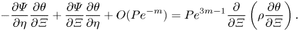 \begin{equation} {-}\frac{\partial \varPsi}{\partial \eta}\frac{\partial \theta}{\partial \varXi} +\frac{\partial \varPsi}{\partial \varXi}\frac{\partial \theta}{\partial \eta} +O({Pe}^{{-}m}) = {Pe}^{3m-1} \frac{\partial}{\partial \varXi} \left(\rho \frac{\partial \theta}{\partial \varXi}\right). \end{equation}
The first two terms in (2.15) are  $O(1)$ and thus $m=1/3$, as expected.
We can now solve (2.15) with the well-known von Mises transformation. Adopting the change of variables  $(\varXi ,\eta ,\zeta ) \rightarrow (\varPsi ,\eta ,\zeta )$, we have
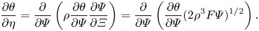 \begin{equation} \frac{\partial \theta}{\partial \eta} = \frac{\partial}{\partial \varPsi}\left( \rho \frac{\partial \theta}{\partial \varPsi} \frac{\partial \varPsi}{\partial \varXi} \right) = \frac{\partial}{\partial \varPsi}\left( \frac{\partial \theta}{\partial \varPsi}(2\rho^3 F\varPsi)^{1/2} \right). \end{equation}
Equation (2.16) now admits a self-similar solution of the form  $\theta = \theta (\chi ), \chi = \varPsi ^{1/2}/\tau ^{1/3}$, where the functions $\theta (\chi )$ and $\tau (\eta )$ must satisfy
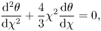 \begin{equation} \frac{\mathrm{d}^2 \theta}{\mathrm{d} \chi^2} + \frac{4}{3}\chi^2 \frac{\mathrm{d} \theta}{\mathrm{d} \chi} = 0, \end{equation}
for
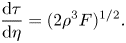 \begin{equation} \frac{\mathrm{d}\tau}{\mathrm{d}\eta} = (2\rho^3 F)^{1/2}. \end{equation}
The solution of (2.17) satisfying the imposed boundary conditions (2.2) of  $\theta (0) = 1$ and $\theta = 0$ as $\chi \rightarrow \infty$ is
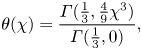 \begin{equation} \theta(\chi) = \frac{\varGamma(\frac{1}{3}, \frac{4}{9} \chi^3)}{\varGamma(\frac{1}{3},0)}, \end{equation}
where  $\varGamma$ is the incomplete gamma function. We can obtain $\tau$ by integrating (2.18) along the surface streamlines, which must begin and terminate at critical points $F=0$ on the surface, since the surface shear stress is continuous. We will therefore choose the constant of integration so that
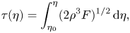 \begin{equation} \tau(\eta) = \int_{\eta_0}^{\eta} (2\rho^3 F)^{1/2}\, \mathrm{d}\eta, \end{equation}
has  $\tau (\eta _0) = 0$ at the beginning of the surface streamline $\eta =\eta _0$ and $\tau (\eta _1) = \tau _1$ at the end $\eta = \eta _1$.
At the surface, the local flux of material per unit area is
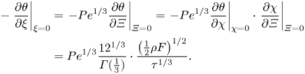 \begin{align} {-}\left.\frac{\partial \theta}{\partial \xi}\right|_{\xi = 0} &=\left. -{Pe}^{1/3} \frac{\partial \theta}{\partial \varXi}\right|_{\varXi=0} = \left.-{Pe}^{1/3} \frac{\partial \theta}{\partial \chi}\right|_{\chi=0} \cdot\left.\frac{\partial \chi}{\partial \varXi}\right|_{\varXi=0} \nonumber\\ &= {Pe}^{1/3} \frac{12^{1/3}}{\varGamma(\frac{1}{3})} \cdot \frac{\left(\frac{1}{2}\rho F\right)^{1/2}}{\tau^{1/3}}. \end{align}
The Sherwood number (2.3) is therefore given by
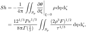 \begin{align} {Sh}&={-}\frac{1}{4{\rm \pi}} \left.\iint_{S_p} \frac{\partial \theta}{\partial \xi}\right|_{\xi=0} \rho\,\mathrm{d}\eta \,\mathrm{d}\zeta \nonumber\\ &= \frac{12^{1/3} {Pe}^{1/3}}{8{\rm \pi} \varGamma(\frac{1}{3})} \iint_{S_p} \frac{(2 \rho^3 F)^{1/2}}{\tau^{1/3}}\, \mathrm{d}\eta \,\mathrm{d}\zeta, \end{align}
which we can integrate by parts by recognising that
 \begin{equation} \int_{\eta_0}^{\eta_1} \frac{\left(2 \rho^3 F\right)^{1/2}}{\tau^{1/3}}\, \mathrm{d}\eta =\int_{\eta_0}^{\eta_1} \frac{\mathrm{d}\tau}{\mathrm{d}\eta} \tau^{{-}1/3}\, \mathrm{d}\eta =\frac{3}{2} \tau_1^{2/3}, \end{equation}
and thus
 \begin{equation} {Sh}= \frac{0.808 {Pe}^{1/3}}{4{\rm \pi}} \int \left( \int_{\eta_0}^{\eta_1} \rho^{3/2} F^{1/2}\, \mathrm{d}\eta \right)^{2/3}\mathrm{d}\zeta + O(1). \end{equation}
As expected, the limiting dimensionless flux scales as  $\alpha {Pe}^{1/3}$, with a prefactor $\alpha$ which can now be explicitly computed in terms of the shape of the body and the surface velocity gradient.
The main point of (2.24) is that we have generalised the results of Acrivos & Goddard (Reference Acrivos and Goddard1965) and Batchelor (Reference Batchelor1979) to any distribution of surface streamlines on an arbitrary body, not just those which result in an orthogonal coordinate system. The caveat remains that the pathlines around the body should be open for the boundary layer approximation to hold and the boundary should be smooth and contain no regions of extreme curvature. Furthermore, we have a natural way of numerically constructing the local area density  $\rho$, as shown graphically in figure 1. By integrating (2.5a–c) with respect to $\eta$ to generate a set of surface streamlines over the body, we obtain lines of constant $\zeta$ at intervals of varying $\eta$. With a sufficiently fine discretisation, we can numerically approximate the local area density $\rho$ and evaluate the coefficient in (2.24) numerically. We shall demonstrate this procedure later in § 3.
2.3. Unsteady solution at large Péclet number
We now seek to generalise our steady solution to an unsteady, periodic flow. Our argument is analogous to that proposed by Batchelor (Reference Batchelor1980), who examined the scalar flux to spherical particles in turbulent flow.
We shall consider the case where the motion is periodic with period  $T = E^*T^*$. We seek the time average Sherwood number $\overline{\textit{Sh}}$ at the surface, which depends upon the time average concentration field $\overline{\theta }$. The time average over a period $T$ is defined simply as
 \begin{equation} \overline{\theta }(\boldsymbol{x}) = \frac{1}{T} \int_{0}^{T} \theta(\boldsymbol{x},t) \mathrm{d}t. \end{equation}
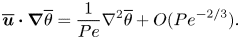
Applying this averaging procedure to (2.1), we obtain
 \begin{equation} \overline{\boldsymbol{u}} \boldsymbol{\cdot} \boldsymbol{\nabla}\overline{\theta } + \overline{\boldsymbol{u}' \boldsymbol{\cdot} \boldsymbol{\nabla} \theta'} = \frac{1}{{Pe}} \nabla^2 \overline{\theta }, \end{equation}
where we have decomposed the velocity field  $\boldsymbol {u} = \overline {\boldsymbol {u}} + \boldsymbol {u}'$ and concentration field $\theta =\overline{\theta }+\theta '$ into their respective average and fluctuating components. Likewise, the transport equation for the concentration fluctuation $\theta '(\boldsymbol {x}, t)$ is
 \begin{equation} \frac{\partial \theta'}{\partial t} + \boldsymbol{u}\boldsymbol{\cdot}\boldsymbol{\nabla} \theta' - \overline{\boldsymbol{u}'\boldsymbol{\cdot}\boldsymbol{\nabla} \theta'} - \frac{1}{{Pe}} \nabla^2 \theta' ={-}\boldsymbol{u}'\boldsymbol{\cdot} \boldsymbol{\nabla} \overline{\theta }. \end{equation}
We shall argue that the solution of (2.27) satisfying the boundary conditions (2.2) and
 \begin{equation} \theta' = 0 \text{ at } \xi = 0 \quad\text{and} \quad \theta' = 0 \text{ as } \xi \rightarrow \infty, \end{equation}
is such that  $\theta ' \sim {Pe}^{-1/3}$ as ${Pe} \rightarrow \infty$. As before, we reason that the solution consists of a slender concentration boundary layer of thickness $\delta /r \sim {Pe}^{-1/3}$. Outside the boundary layer $\xi \gg \delta$, $\overline{\theta } \rightarrow 0$ and $\theta ' \rightarrow 0$. Inside the boundary layer, the amplitude of the concentration fluctuations are $\theta ' = O({Pe}^{m'})$ and the jump in the mean concentration across the boundary layer is $O(1)$. Clearly, $m' \le 0$ since there is no mechanism in (2.1) which can amplify scalar fluctuations. If $m' < 0$, then scalar fluctuations should decay in amplitude at large ${Pe}$, whereas if $m' = 0$ they remain comparable in magnitude to the mean flow.
Let us examine the order of magnitude of the terms in (2.27). Since scalar fluctuations are  $O({Pe}^{m'})$ and occur on a time scale of $O(T)$, the time derivative term scales as
 \begin{equation} \frac{\partial \theta}{\partial t} \sim \frac{{Pe}^{m'}}{T}. \end{equation}
The convective terms on the left-hand side scale as
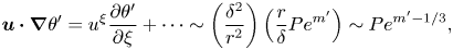 \begin{equation} \boldsymbol{u}\boldsymbol{\cdot} \boldsymbol{\nabla} \theta' = u^\xi \frac{\partial \theta'}{\partial \xi} + \cdots \sim \left(\frac{\delta^2}{r^2}\right) \left(\frac{r}{\delta} {Pe}^{m'} \right) \sim {Pe}^{m'-1/3}, \end{equation}
whereas the convective term on the right-hand side scales as
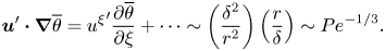 \begin{equation} \boldsymbol{u}' \boldsymbol{\cdot} \boldsymbol{\nabla} \overline{\theta } = {u^\xi}' \frac{\partial \overline{\theta }}{\partial \xi} + \cdots \sim \left(\frac{\delta^2}{r^2}\right) \left(\frac{r }{\delta}\right) \sim {Pe}^{{-}1/3}. \end{equation}
Finally, the diffusion term scales as
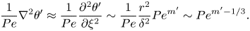 \begin{equation} \frac{1}{{Pe}}\nabla^2 \theta' \approx \frac{1}{{Pe}} \frac{\partial^2 \theta'}{\partial \xi^2} \sim \frac{1}{{Pe}} \frac{r^2}{\delta^2} {Pe}^{m'} \sim {Pe}^{m' - 1/3}. \end{equation}
Annotating (2.27) with the order of magnitude of each term, we have
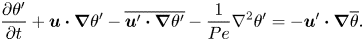
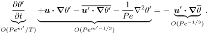 \begin{equation} \underbrace{\frac{\partial \theta'}{\partial t}}_{O({Pe}^{m'}/T)} \underbrace{ + \boldsymbol{u}\boldsymbol{\cdot}\boldsymbol{\nabla} \theta' - \overline{\boldsymbol{u}'\boldsymbol{\cdot}\boldsymbol{\nabla} \theta'} - \frac{1}{{Pe}} \nabla^2 \theta' }_{O({Pe}^{m'-1/3})} ={-}\underbrace{\boldsymbol{u}'\boldsymbol{\cdot} \boldsymbol{\nabla} \overline{\theta }}_{O({Pe}^{{-}1/3})}. \end{equation}
We see that the solution requires  $m'=-1/3$, such that the first term on the left-hand side dominates and balances the unsteady convection term on the right-hand side, provided the dimensionless period $T \ll {Pe}^{1/3}$. Thus, at large Péclet, we have
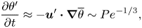 \begin{equation} \frac{\partial \theta'}{\partial t} \approx{-}\boldsymbol{u}'\boldsymbol{\cdot} \boldsymbol{\nabla} \overline{\theta } \sim {Pe}^{{-}1/3}, \end{equation}
which is equivalent to (3.9) of Batchelor (Reference Batchelor1980). However, we have derived the result on more general grounds. Physically, this result means that when the time scale of diffusion within the boundary layer becomes large in comparison to the time scale of the unsteadiness, there is insufficient time for diffusion to redistribute scalar fluctuations. Instead, scalar fluctuations inside the boundary layer occur due to the convection of the mean concentration field by unsteady velocity fluctuations.
Thus, to leading order, the concentration and its time mean are equal and the mean scalar field is well approximated by
 \begin{equation} \overline{\boldsymbol{u}}\boldsymbol{\cdot}\boldsymbol{\nabla}\overline{\theta } = \frac{1}{{Pe}}\nabla^2 \overline{\theta } + O({Pe}^{{-}2/3}). \end{equation}
This allows us to apply our general result (2.24) to unsteady, time periodic flows where the period of motion is sufficiently small. As before, for the boundary layer approximation to hold, it is required that the surface of the particle be exposed to a continuous stream of fresh fluid. Therefore, it is required that the pathlines of fluid parcels adjacent to the surface be open, such that the fluid does not simply recirculate around a closed path.
3. The steady flux for a spheroid
We shall now apply the results of § 2.2 to obtain the scaling coefficient  $\alpha$ for a spheroid in an arbitrary linear shear. Although the motion is in general unsteady, we have argued in § 2.2 that the average mass transfer rate can be computed for an equivalent spheroid subject to the same average relative flow field. This flow field can be described by three parameters, but for a broad class of cases, the flow is reduced to an axisymmetric configuration described by a single parameter. To proceed, we shall analyse the relative motion of the particle in § 3.1 and obtain expressions for the average flow field perceived by the particle. We introduce an expression for the velocity field near the particle in § 3.2, then derive the mass transfer coefficient in the axisymmetric and general cases in §§ 3.3 and 3.4 respectively. Based on these results, we consider the special case of rotation-dominated flow in § 3.5 and discuss potential extensions in § 3.6.
3.1. Motion of a freely suspended spheroid
Let us consider the motion of a spheroidal particle in an arbitrary, linear shear flow. The background linear shear is  $\boldsymbol {v} = \boldsymbol{\mathsf{G}}\boldsymbol{y}$, where $\boldsymbol {y}=\boldsymbol {y}^*/r$ is the coordinate system of the fixed laboratory frame and $\boldsymbol{\mathsf{G}} = \boldsymbol{\mathsf{E}} + \boldsymbol{\mathsf{W}}$ is an arbitrary, steady velocity gradient in this reference frame. The velocity gradient is composed of a symmetric strain tensor $\boldsymbol{\mathsf{E}}=\boldsymbol{\mathsf{E}}^*/E^*$ and antisymmetric rotation tensor $\boldsymbol{\mathsf{W}}=\boldsymbol{\mathsf{W}}^*/E^*$. We shall choose the characteristic shear rate ${\mathsf{E}}^* = ({\mathsf{E}}_{ij}^*{\mathsf{E}}_{ij}^*)^{1/2}$ so that ${\mathsf{E}}_{ij}{\mathsf{E}}_{ij}=1$.
The spheroid is centred at the origin and its semiaxes  $a_i = (a,c,c)$ are spanned by an orthogonal set of unit vectors $\boldsymbol {p},\boldsymbol {q},\boldsymbol {r}$. Thus, the coordinate $\boldsymbol {x}$ in the body frame maps to the laboratory frame as $\boldsymbol {y} = \boldsymbol{\mathsf{R}}\boldsymbol {x}$, where $\boldsymbol{\mathsf{R}} = [\boldsymbol {p}, \boldsymbol {q}, \boldsymbol {r}]$. The unit vector $\boldsymbol {p}$ points along the symmetry axis towards the ‘pole’ of the spheroid, whilst $\boldsymbol {q}$ and $\boldsymbol {r}$ point radially outward around the ‘equator’. The body rotates with angular velocity $\boldsymbol {\varOmega }=\boldsymbol {\varOmega }(t)$, such that $\dot {\boldsymbol{\mathsf{R}}} = [\boldsymbol {\varOmega }]_\times \boldsymbol{\mathsf{R}}$, and the velocity field in the body frame is
 \begin{equation} \boldsymbol{u}(\boldsymbol{x},t) = \boldsymbol{\mathsf{R}}^\textrm{T}\boldsymbol{v}(\boldsymbol{\mathsf{R}}\boldsymbol{x},t) - \boldsymbol{\varOmega}\times(\boldsymbol{\mathsf{R}}\boldsymbol{x}). \end{equation}
Thus, the background velocity gradient  $\boldsymbol {u}=\boldsymbol{\mathsf{A}}\kern1.5pt\boldsymbol {x}$ appears in the body frame as
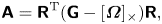 \begin{equation} \boldsymbol{\mathsf{A}} = \boldsymbol{\mathsf{R}}^\textrm{T} (\boldsymbol{\mathsf{G}} - [\boldsymbol{\varOmega}]_\times) \boldsymbol{\mathsf{R}}, \end{equation}
and, in general, varies in time as the particle rotates. Jeffery (Reference Jeffery1922) showed that, when the couple upon a spheroid is zero, the solid body rotation rate  $\boldsymbol {\varOmega }$ of the body is given by
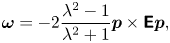
 \begin{equation} \boldsymbol{\varOmega} = \frac{1}{2}\boldsymbol{\omega} + \frac{\lambda^2-1}{\lambda^2+1} \boldsymbol{p}\times \boldsymbol{\mathsf{E}}\boldsymbol{p}, \end{equation}
where  $\omega _i = -\epsilon _{ijk}{\mathsf{W}}_{jk}$ is the background vorticity in the laboratory frame. Thus, the orientation of the particle $\boldsymbol {p}$ then evolves according to Jeffery's equation
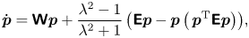 \begin{equation} \dot{\boldsymbol{p}} = \boldsymbol{\mathsf{W}}\boldsymbol{p} + \frac{\lambda^2-1}{\lambda^2+1} \left(\boldsymbol{\mathsf{E}}\boldsymbol{p} - \boldsymbol{p}\left(\kern1.5pt\boldsymbol{p}^\textrm{T}\boldsymbol{\mathsf{E}}\boldsymbol{p}\right)\right)\!, \end{equation}
where  ${\mathsf{W}}_{ij} = \frac {1}{2}\epsilon _{ijk}\omega _k$ is the rate of rotation tensor.
When the background shear is constant in time, the solution to (3.4) can be written in terms of a matrix exponential as
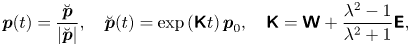 \begin{equation} \boldsymbol{p}(t) = \frac{\breve{\boldsymbol{p}}}{|\breve{\boldsymbol{p}}|}, \quad \breve{\boldsymbol{p}}(t) = \exp\left(\boldsymbol{\mathsf{K}}t\right) \boldsymbol{p}_0, \quad \boldsymbol{\mathsf{K}} = \boldsymbol{\mathsf{W}} + \frac{\lambda^2-1}{\lambda^2+1}\boldsymbol{\mathsf{E}}, \end{equation}
subject to the initial condition  $\boldsymbol {p}=\boldsymbol {p}_0$ at $t=0$ (Szeri Reference Szeri1993).
We shall now examine the fixed points and stable attractors of (3.4). This analysis elaborates upon the previous work by Bretherton (Reference Bretherton1962). Decomposing  $\boldsymbol{\mathsf{K}}$ in terms of its eigenvectors $\boldsymbol {e}_i$ and eigenvalues $\lambda _i$, we can write (3.5a–c) as
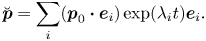 \begin{equation} \breve{\boldsymbol{p}} = \sum_i (\boldsymbol{p}_0\boldsymbol{\cdot}\boldsymbol{e}_i) \exp(\lambda_i t) \boldsymbol{e}_i. \end{equation}
From (3.6) we see that the fixed points of (3.4) coincide with the eigenvectors  $\boldsymbol {e}_i$. The stability of the fixed points depends upon the eigenvalues $\lambda _i$, and because $\sum _i \lambda _i =0$, there is always only one (neutrally) stable fixed point or limit cycle (excepting $\lambda _i=0$). Thus after a finite time, the motion of the particle will always approach a stable attractor whose nature depends upon the largest eigenvalue(s) of $\boldsymbol{\mathsf{K}}$.
We can categorise the stable attractors into five different cases: 1a, 1b, 2a, 2b and 3. These five cases map to four different motions: resting, spinning, 2-D (two-dimensional) tumbling and 3-D (three-dimensional) tumbling. These are summarised in table 1. We shall now examine each case.
Table 1. Classification of the motion and time average perceived velocity gradient experienced by a spheroid.
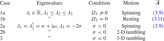
In cases 1a and 1b, all the eigenvalues  $\lambda _1 \le \lambda _2 \le \lambda _3$ of $\boldsymbol{\mathsf{K}}$ are real and (3.5a–c) has three fixed points $\boldsymbol {p} = \boldsymbol {e}_i$, where $\boldsymbol {e}_i$ are the eigenvectors of $\boldsymbol{\mathsf{K}}$. From (3.6) we see that only the fixed point corresponding to the largest eigenvalue $\lambda _3$ is stable, so for nearly any initial condition, the particle will reorient itself to be parallel to $\boldsymbol {e}_3$. In this configuration, the particle will in general rotate about its axis with angular velocity $\boldsymbol {\varOmega } = \varOmega _3 \boldsymbol {e}_3$, where $\varOmega _3 = \boldsymbol {\omega }\boldsymbol {\cdot }\boldsymbol {e}_3/2$ (case 1a). We call this motion spinning. However, for particular configurations, $\varOmega _3 = 0$ and the particle does not rotate (case 1b). We call this motion resting.
In cases 2a, 2b and 3,  $\boldsymbol{\mathsf{K}}$ has a pair of complex eigenvalues and the system has one fixed point and a periodic point. In these cases, we can write the eigenvalues as $\lambda _1 = \lambda _2^{\dagger}ger = \sigma + \textrm {i}\omega , \lambda _3 = -2\sigma$, where ${\dagger}ger$ denotes the complex conjugate. When $\sigma < 0$, the fixed point is stable and the periodic point is unstable (case 2a, spinning). Thus the particle aligns with $\boldsymbol {e}_3$ as in cases 1a and 1b, but unlike case 1b, the particle must rotate about this axis because the angular velocity $\boldsymbol {\varOmega } = \varOmega _3 \boldsymbol {e}_3$ is bounded $\varOmega _3^2 \ge \omega ^2 > 0$. When $\sigma > 0$, the fixed point is unstable and the periodic point is stable (case 2b). Thus the particle will evolve towards a planar limit cycle oscillation described by
 \begin{equation} \breve{\boldsymbol{p}} = \boldsymbol{a}\cos(\omega t) + \boldsymbol{b}\sin(\omega t), \end{equation}
where  $\boldsymbol {e}_1 = \boldsymbol {e}_2^{\dagger}ger = \boldsymbol {a}+\textrm {i}\boldsymbol {b}$. We call this motion 2-D tumbling. In case 3, $\sigma = 0$ and the motion follows 3-D Jeffery orbits (Jeffery Reference Jeffery1922), where $\boldsymbol {p}$ precesses around the axis $\boldsymbol {e}_3$ with period $2{\rm \pi} /\omega$. We call this motion 3-D tumbling (Jeffery orbits are in general three-dimensional, but for some initial conditions, the motion can be reduced to spinning or 2-D tumbling).
The solution of (2.26) depends upon the average flow field in the particle frame. The instantaneous flow field around the particle consists of a superposition of the background gradient  $\boldsymbol{\mathsf{A}}\kern0.09em \boldsymbol {x}$ and a perturbation owing to the presence of the particle. Since this perturbation is linear in $\boldsymbol{\mathsf{A}}$, the time average flow field in the particle frame is determined by the average velocity gradient perceived by the particle. We shall now calculate the average velocity gradient perceived by the particle in the general limiting cases identified above.
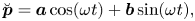
In cases 1a and 2a (spinning), the particle rotates around a fixed axis  $\boldsymbol {p}=\boldsymbol {e}_3$, which is illustrated in figure 2(a). For this spinning motion, the unit vectors of the body frame rotate as
 \begin{equation} \boldsymbol{p} = \boldsymbol{e}_3,\quad \boldsymbol{q} = \cos(\varOmega_3 t) \boldsymbol{q}_0 + \sin(\varOmega_3 t) \boldsymbol{r}_0, \quad \boldsymbol{r} ={-}\sin(\varOmega_3 t) \boldsymbol{q}_0 + \cos(\varOmega_3 t) \boldsymbol{r}_0. \end{equation}
To obtain the time average velocity gradient, we can substitute (3.8a–c) into (3.2) and take the time average over one revolution, whose period is  $T = 2{\rm \pi} /\varOmega _3$. After a little algebra, we obtain
 \begin{equation} \overline{\boldsymbol{\mathsf{A}}} = \frac{1}{T} \int_{0}^T \boldsymbol{\mathsf{R}}^\textrm{T}(\boldsymbol{\mathsf{G}}-[\boldsymbol{\varOmega}]_\times)\boldsymbol{\mathsf{R}}\, \mathrm{d}t = E_3 \begin{bmatrix} 1 & 0 & 0 \\ 0 & -\frac{1}{2} & 0 \\ 0 & 0 & -\frac{1}{2} \end{bmatrix}, \end{equation}
where
 \begin{equation} E_3 = \boldsymbol{e}_3^\textrm{T}\boldsymbol{\mathsf{E}}\boldsymbol{e}_3 = \frac{\lambda^2+1}{\lambda^2-1} \sigma, \end{equation}
is the rate of strain perceived by the particle along its fixed axis of rotation. Thus, the average velocity field experienced by a particle steadily rotating about its axis is an axisymmetric strain, whose magnitude is given by the component of strain along the rotation axis.
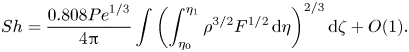
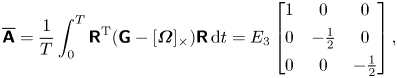
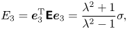
Figure 2. Motion of a freely suspended spheroid: (a) spinning, (b) 2-D tumbling and (c) 3-D tumbling. For 2-D tumbling and spinning, the motion is periodic, whereas for 3-D tumbling only the motion of the symmetry axis is necessarily periodic.
In case 1b (resting), the particle axis aligns with  $\boldsymbol {e}_3$, but the rotation rate about this axis vanishes. The average velocity field in the body frame is then simply
 \begin{equation} \overline{\boldsymbol{\mathsf{A}}} = \boldsymbol{\mathsf{RGR}}^{T}. \end{equation}
The average velocity gradient  $\overline {\boldsymbol {A}}$ can be specified with three parameters, up to an arbitrary scaling and rotation about the symmetry axis of the particle. To see this, we note that $\boldsymbol{\mathsf{G}}$ has nine components with eight degrees of freedom, since continuity requires $\textrm {tr}(\boldsymbol{\mathsf{G}}) = 0$. The requirement that $\boldsymbol {\varOmega } = 0$ imposes the constraint
 \begin{equation} \boldsymbol{\omega} ={-}2\frac{\lambda^2-1}{\lambda^2+1} \boldsymbol{p}\times \boldsymbol{\mathsf{E}}\boldsymbol{p}, \end{equation}
reducing the number of unknowns by three. The choice of scale introduces another redundant parameter; our non-dimensionalisation requires  ${\mathsf{E}}_{ij}{\mathsf{E}}_{ij} = 1$. Finally, we note that rotations about the particle's axis are trivial, since the particle is axisymmetric.
In case 2b (2-D tumbling), the motion of the particle is more complex, but remains periodic, as illustrated in figure 2(b). From (3.7) it follows that the symmetry axis  $\boldsymbol {p}$ rotates in a plane spanned by vectors $\boldsymbol {a},\boldsymbol {b}$ with period $T = 2{\rm \pi} /\omega$. Thus the rotation $\boldsymbol{\mathsf{Q}}(t) = \boldsymbol{\mathsf{Q}}_2\boldsymbol{\mathsf{Q}}_1$ of the body frame $\boldsymbol{\mathsf{R}}(t) = \boldsymbol{\mathsf{Q}}\boldsymbol{\mathsf{R}}_0$ can be composed of as a rotation $\boldsymbol{\mathsf{Q}}_1(t)$ about the axis $\boldsymbol {a}\times \boldsymbol {b}$ (mapping $\boldsymbol {p}_0$ onto $\boldsymbol {p}$), followed by a rotation $\boldsymbol{\mathsf{Q}}_2(t)$ about the axis $\boldsymbol {p} = \boldsymbol{\mathsf{Q}}_1\boldsymbol {p}_0$ by an angle
 \begin{equation} \theta_p(t) = \int_{0}^{t} \frac{1}{2} \boldsymbol{\omega}\boldsymbol{\cdot} \boldsymbol{p}(t') \mathrm{d}t', \end{equation}
relative to the plane normal. By inspection of (3.13) and (3.7), we see that  $\theta _p(T) = 0$, since $\boldsymbol {p}(t) = -\boldsymbol {p}(t+T/2)$. Thus, $\boldsymbol{\mathsf{R}}(t)$ must be periodic. The average perceived velocity gradient can then be evaluated analogously to (3.9), but the resultant expression is much more complicated. It suffices to remark that the average strain $\overline{\boldsymbol{\mathsf{E}}}$ and vorticity $\overline{\boldsymbol{\omega}}$ components of the average perceived velocity gradient $\overline{\boldsymbol{\mathsf{A}}}$ must also satisfy (3.12), since in the body frame, the apparent rotation rate of the body must also be zero. It follows that in case 2b, as in case 1b, the average perceived velocity gradient may also be described by only three parameters, up to a trivial rotation and choice of scale.
In case 3 (3-D tumbling), the particle motion becomes fully three dimensional, as illustrated in figure 2(c). Only the motion of its symmetry axis is necessarily periodic; the equatorial axes  $\boldsymbol {q}$ and $\boldsymbol {r}$ may precess around and do not necessarily trace a path with the same period. Thus, we cannot expect the flow in the particle frame to be time periodic, since $\boldsymbol {q}$ and $\boldsymbol {r}$ point in a new direction at the start of each cycle, and we cannot expect to apply (2.24) in this special case.
We recall that the derivation of (2.24) required pathlines of the flow to be open. Far from the particle, pathlines follow  $\dot {\boldsymbol {y}} = \boldsymbol{\mathsf{G}}\boldsymbol{y}$, with solution $\boldsymbol {y} = \exp (\boldsymbol{\mathsf{G}}t)\boldsymbol {y}_0$. By a similar argument to that above, we see that when $\boldsymbol{\mathsf{G}}$ has eigenvalues $0,\pm \mathrm {i}\omega$, the pathlines are closed. This provides a necessary condition to apply (2.24). The 3-D tumbling orbits identified by Jeffery (Reference Jeffery1922) happen to correspond to this case, which further precludes application of (2.24) to the case of Jeffery orbits.
To summarise: by an analysis of the stable attractors of (3.4) we can construct five cases of the particle motion categorised by the eigenvalues of  $\boldsymbol{\mathsf{K}}$ (3.5a–c) as shown in table 1. In cases 1a, 1b and 2a, the particle orients itself along a fixed axis corresponding to the eigenvector $\boldsymbol{\mathsf{K}}$ with largest real eigenvalue. In cases 2b and 3, the particle undergoes a limit cycle oscillation. In cases 1a, 1b, 2a and 2b, the relative flow field is steady or periodic. In cases 1a, 2a (spinning) the average perceived velocity gradient over one period is an axisymmetric strain, because the particle rotates steadily about its axis. In cases 1b and 2b (resting or 2-D tumbling), the average perceived velocity gradient satisfies (3.12), which can be specified in terms of three parameters up to a trivial rotation and choice of scale.
3.2. The fluid motion near the particle
In the body frame, the surface at  $\xi = 0$ is stationary, so to leading order in $\xi$ the velocity is
 \begin{equation} \boldsymbol{u} = \xi \left.\frac{\partial \boldsymbol{u}}{\partial \xi}\right|_{\xi = 0} + O(\xi^2). \end{equation}
After differentiation of Jeffery's solution for the relative velocity field for an arbitrary ellipsoid (Jeffery Reference Jeffery1922), rewritten in the more compact matrix notation used by Kim & Karrila (Reference Kim and Karrila1991), we find that the velocity gradient normal to the surface is given by
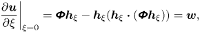 \begin{equation} \left.\frac{\partial \boldsymbol{u}}{\partial \xi}\right|_{\xi=0} = \boldsymbol{\Phi}\boldsymbol{h}_\xi - \boldsymbol{h}_\xi(\boldsymbol{h}_\xi \boldsymbol{\cdot} (\boldsymbol{\Phi}\boldsymbol{h}_\xi)) = \boldsymbol{w}, \end{equation}
where  $\boldsymbol {h}_\xi = \boldsymbol{\mathsf{D}}\boldsymbol {x}/|\boldsymbol{\mathsf{D}}\boldsymbol{x}|$ is the unit vector surface normal, $\boldsymbol{\mathsf{D}}$ is a diagonal matrix whose entries are $a_i^{-2}$ and
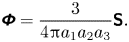 \begin{equation} \boldsymbol{\Phi} = \frac{3}{4{\rm \pi} a_1 a_2 a_3}\boldsymbol{\mathsf{S}}. \end{equation}
The expression for the stresslet  $\boldsymbol{\mathsf{S}}$ is more involved. We remark here that it is a symmetric matrix with $\textrm {tr}(\boldsymbol{\mathsf{S}}) = 0$ whose elements are a linear combination of the components of the velocity gradient $\boldsymbol{\mathsf{A}}$ with coefficients determined by geometry-dependent ‘resistance functions’. Complete expressions for $\boldsymbol{\mathsf{S}}$ can be found in Kim & Karrila (Reference Kim and Karrila1991). Equation (3.15) is valid for the general case of torque-free, tri-axial ellipsoids. The action of a net torque upon the body adds an additional skew–symmetric component to (3.16) which is not treated here.
Equation (3.15) now defines the surface streamlines, which are everywhere tangent to the surface velocity gradient  $\boldsymbol {w}$. The surface streamlines and their critical points are illustrated for an arbitrary linear shear in figure 1. From (3.15) we see that critical points occur where the surface normal $\boldsymbol {h}_\xi$ coincides with an eigenvector $\pm \boldsymbol {q}_i$ of the surface gradient tensor $\boldsymbol{\Phi}$. Since $\boldsymbol{\Phi}$ is a symmetric matrix, its eigenvalues are all real and its eigenvectors orthogonal. In general, $\boldsymbol{\Phi}$ has three distinct eigenvalues ordered $\phi _1 < \phi _2 < \phi _3$ and there are six critical points. In special cases, $\boldsymbol{\Phi}$ has a repeated eigenvalue and there is a locus of critical points.
The precise nature of the critical points can be seen by introducing the surface potential
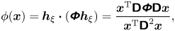 \begin{equation} \phi(\boldsymbol{x}) = \boldsymbol{h}_\xi \boldsymbol{\cdot} (\boldsymbol{\Phi}\boldsymbol{h}_\xi) = \frac{\boldsymbol{x}^\textrm{T}\boldsymbol{\mathsf{D}}\boldsymbol{\Phi} \boldsymbol{\mathsf{D}}\boldsymbol{x}}{\boldsymbol{x}^\textrm{T}\boldsymbol{\mathsf{D}}^2\boldsymbol{x}}, \end{equation}
which has the property that
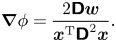 \begin{equation} \boldsymbol{\nabla} \phi = \frac{2\boldsymbol{\mathsf{D}}\boldsymbol{w}}{\boldsymbol{x}^\textrm{T}\boldsymbol{\mathsf{D}}^2\boldsymbol{x}}. \end{equation}
The gradient of  $\phi$ measured along surface streamlines is $\boldsymbol {w}\boldsymbol {\cdot }\boldsymbol {\nabla } \phi > 0$ everywhere on the surface except at the critical points $\boldsymbol {w}=0$ where the surface streamlines terminate. In other words, the potential $\phi$ always increases as one moves along a surface streamline. The potential takes a minimum value of $\phi = \phi _1$ when $\boldsymbol {h}_\xi = \pm \boldsymbol {q}_1$ (red marker in figure 1), i.e. surface streamlines originate from a ‘source’ $\phi = \phi _1$. It takes a maximum value of $\phi = \phi _3$ when $\boldsymbol {h}_\xi = \pm \boldsymbol {q}_3$ (blue marker), i.e. surface streamlines terminate at a ‘sink’ $\phi = \phi _3$. Lastly, when the eigenvalues are distinct, all streamlines must pass through the contour $\phi = \phi _2$, except at points $\boldsymbol {h}_\xi = \pm \boldsymbol {q}_2$, which are saddle points (green marker). When there is a repeated eigenvalue, either $\phi _2 = \phi _1$ or $\phi _2 = \phi _3$, so there exists a locus of points where streamlines originate (or terminate). It should be noted that the definition of $\phi$ (3.17) and its properties extend also to torque-free, tri-axial ellipsoids.
3.3. Surface flux under spinning motion
We now proceed to evaluate the surface streamlines about a spheroid aligned with the axis of an axisymmetric straining flow. This configuration corresponds to the mean flow field about a spinning spheroid. In the body frame, the velocity gradient tensor is a diagonal matrix whose elements are  ${\mathsf{A}}_{11}/2 = -{\mathsf{A}}_{22} = -{\mathsf{A}}_{33} = {\mathsf{E}}_3$. Likewise, the surface velocity gradient tensor $\boldsymbol{\Phi}$ is also a diagonal matrix with $\varPhi _{11}/2 = -\varPhi _{22} = -\varPhi _{33} = \beta E_3/2$, where the geometry-dependent prefactor $\beta$ is given by
 \begin{equation} \frac{1}{\beta} = \frac{3}{4} \int_{0}^{\infty} \frac{ac^2 t}{(a^2+t)^{3/2}(c^2+t)^2}\, \mathrm{d}t. \end{equation}
 For this configuration, the surface streamlines are axisymmetric, originating at the ‘pole’ and terminating at the ‘equator’. Therefore, we can use an ellipsoidal polar coordinate system to describe the surface, identifying  $\eta$ with the polar angle between the symmetry axis and a point on the surface and $\zeta$ with the azimuthal angle. We parametrise a point near the surface as
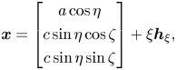 \begin{equation} \boldsymbol{x} = \begin{bmatrix} a\cos\eta \\ c\sin\eta\cos\zeta \\ c\sin\eta\sin\zeta \end{bmatrix} +\xi\boldsymbol{h}_\xi, \end{equation}
so that the covariant coordinate vectors at the surface are
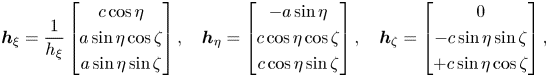 \begin{equation} \boldsymbol{h}_\xi = \frac{1}{h_\xi} \begin{bmatrix} c\cos\eta \\ a\sin\eta \cos\zeta \\ a\sin\eta \sin\zeta\end{bmatrix} ,\quad \boldsymbol{h}_\eta = \begin{bmatrix} -a \sin\eta \\ c\cos\eta \cos\zeta \\ c\cos\eta \sin\zeta \end{bmatrix}, \quad \boldsymbol{h}_\zeta = \begin{bmatrix} 0 \\ -c\sin\eta \sin\zeta \\ +c\sin\eta \cos\zeta \end{bmatrix}, \end{equation}
with  $h_\xi$ chosen to ensure that $\boldsymbol {h}_\xi$ is a unit vector. Then it follows that
 \begin{equation} u^\zeta = 0, \quad u^\eta = \frac{3}{2} \xi |\varPhi_{11}| \frac{ac \cos\eta\sin\eta}{(a^2\sin^2\eta + c^2\cos^2\eta)^{3/2}} = F\xi, \end{equation}
as required and
 \begin{equation} \rho = c \sin\eta(a^2 \sin^2\eta + c^2\cos^2\eta)^{1/2}. \end{equation}
Substituting (3.22a,b) and (3.23) into (2.24), we obtain
 \begin{align} \int_{\eta_0}^{\eta_1} {\rho}^{3/2}{F}^{1/2}\, \mathrm{d}\eta &= \int_{0}^{{\rm \pi}/2} \left( \frac{3}{2}\beta |{E}_{3}| {a}{c}^4 \cos\eta \sin^4\eta \right)^{1/2}\mathrm{d}\eta \nonumber\\ &= \left(\frac{{\rm \pi} {a}{c}^4 \beta |{E}_{3}|}{6}\right)^{1/2} \frac{\varGamma(\frac{7}{4})}{\varGamma(\frac{9}{4})}, \end{align}
and thus
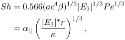 \begin{align} {Sh} &= 0.566 ({a}{c}^4 \beta)^{1/3} |E_3|^{1/3} {Pe}^{1/3} \nonumber\\ &= \alpha_{||}\left(\frac{|E_3|^* r}{\kappa}\right)^{1/3}, \end{align}
where  $\alpha _{||}(\lambda ) = 0.566 ({a}{c}^4 \beta )^{1/3}$ represents the dependence of the surface flux upon geometry and $|E_3|^*r/\kappa$ is the Péclet number based on the strain perceived along the axis of rotation.
The geometry-dependent prefactor  $\alpha _{||}$ has a relatively weak dependence upon the aspect ratio of the spheroid, varying between $0.762$ to $1.042$ over the interval $1/20 \le \lambda \le 20$. In contrast, from the definition of the characteristic shear rate $E^*$, $|E_3|$ may vary over the interval $0 < |E_3| \le 2/\sqrt {6}$, depending on the particular configuration of the background strain and the axis of the particle. Therefore, the alignment of the particle with the background velocity gradient plays a significant role in determining the surface flux for spinning particles. This is the phenomenon of the partial suppression of convection by rotation first identified by Batchelor (Reference Batchelor1979).
Some caution must be taken in utilising the result of (3.25). In our derivation of (2.24), we have assumed that the boundary layer thickness remains small in comparison to radius of curvature of the surface, so that cross-surface diffusion and higher-order convection terms are negligible. Yet, when the body is made infinitely slender, this assumption is violated. We expect that higher-order corrections to (2.24) are required for slender bodies at moderate Péclet number.
3.4. Surface flux under tumbling and resting motion
Under tumbling and resting motion, convenient expressions for the surface streamlines are no longer easy to find by hand. To proceed in this general case, we adopt a numerical approach to parametrise the surface in terms of coordinates  $\boldsymbol {x} = \boldsymbol {x}(0, \eta , \zeta )$. Essentially, the task is to draw a set of $j = 1 \ldots n_\zeta$ surface streamlines covering the body, label each streamline with a unique $\zeta = \zeta _j$ and evaluate the position at $i = 1 \ldots n_\eta$ different locations $\eta = \eta _i$ along the streamline. Then we can create a $n_\eta \times n_\zeta$ mesh of points $\boldsymbol {x}_{i,j} = \boldsymbol {x}(0,\eta _i,\zeta _j)$ upon the surface to numerically approximate the metric $\rho$, which can be used to numerically integrate (2.24).
We shall now construct a suitable definition of the streamwise coordinate  $\eta$. We require the surface streamlines be tangent to the surface velocity gradient $\boldsymbol {w}$ (3.15), so $\boldsymbol {h}_\eta$ must be of the form
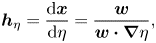 \begin{equation} \boldsymbol{h}_\eta = \frac{\mathrm{d}\boldsymbol{x}}{\mathrm{d}\eta} = \frac{\boldsymbol{w}}{\boldsymbol{w}\boldsymbol{\cdot} \boldsymbol{\nabla} \eta}, \end{equation}
which has  $\boldsymbol {\nabla } \eta \boldsymbol {\cdot } \boldsymbol {h}_\eta = 1$ and $\boldsymbol {h}_\eta \boldsymbol {\cdot } \boldsymbol {h}_\xi = 0$, as required. Furthermore, we require that $\eta$ should increase monotonically along surface streamlines. We have seen in § 3.2 that the surface potential $\phi$ has this property. Therefore, we identify $\phi$ (3.17) with the streamwise coordinate $\eta$.
We require a definition of the  $\zeta$ coordinate. Since $\zeta$ is constant along surface streamlines and every surface streamline passes through $\eta = \phi _2$, $\zeta$ can be thought of as a coordinate along the curve $\boldsymbol {x}_0(\zeta ) = \boldsymbol {x}(0, \phi _2, \zeta )$. Along $\eta = \phi _2$, from (3.17) we derive that the unit surface normal satisfies
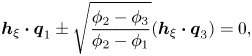 \begin{equation} \boldsymbol{h}_\xi\boldsymbol{\cdot} \boldsymbol{q}_1 \pm \sqrt{\frac{\phi_2 - \phi_3}{\phi_2 - \phi_1}} (\boldsymbol{h}_\xi\boldsymbol{\cdot} \boldsymbol{q}_3) = 0, \end{equation}
so the constraint
 \begin{equation} \zeta = \boldsymbol{h}_\xi \boldsymbol{\cdot} \boldsymbol{q}_2, \end{equation}
describes a point along  $\boldsymbol {x}_0(\zeta )$. The surface can be split into four quadrants, depending upon the basin of attraction of the surface streamlines. To wit, the behaviour in the limits $\boldsymbol {h}_\xi \rightarrow \pm \boldsymbol {q}_1$ as $\eta \rightarrow \phi _1$ and $\boldsymbol {h}_\xi \rightarrow \pm \boldsymbol {q}_3$ as $\eta \rightarrow \phi _3$ forms our classification. Therefore, in each quadrant, the coordinates $(\eta ,\zeta ) \in [\phi _1, \phi _3] \times [-1, 1]$ uniquely define a point on the surface. This definition is general for torque-free, tri-axial ellipsoids.
We now outline the procedure to evaluate (2.24) numerically. For each surface quadrant, we choose a set of points  $\boldsymbol {x}_{0,j} = \boldsymbol {x}(0, \phi _2, \zeta _j)$ which lie on the ellipsoid surface $\xi = 0$ and satisfy $\eta (\boldsymbol {x}) = \phi _2$ (3.17). We numerically integrate (3.26) from the initial condition $\boldsymbol {x}=\boldsymbol {x}_{0,i}$ at $\eta = \phi _2$ to $\eta = \eta _j$, which yields a mesh of points $\boldsymbol {x}_{i,j} = \boldsymbol {x}(0,\eta _i,\zeta _j)$ upon the particle surface. Measuring the surface area $\delta {\mathsf{S}}_{ij}$ of the region enclosed over $[\eta _i,\eta _{i+1}] \times [\zeta _i,\zeta _{i+1}]$, we approximate the surface area density for this surface element as
 \begin{equation} \rho_{ij} \approx \delta {\mathsf{S}}_{ij} (\eta_{i+1}-\eta_i)(\zeta_{i+1}-\zeta_i), \end{equation}
which is, roughly speaking, a ‘cell average’ of  $\rho$. The velocity component $F$ (2.8) is evaluated at $\boldsymbol {x}_{i,j}$ from (3.17) and (3.15). Then, the integral (2.24) is evaluated as a Riemann sum over the surface elements.
A technical point remains that  $\eta _i$ and $\zeta _j$ should be chosen so that the surface is densely covered in mesh points $\boldsymbol {x}_{i,j}$. To achieve this, we generate a uniform sampling of seed points on the surface. These seed points can be integrated (3.26) numerically towards the curve $\boldsymbol {x}_0$ to construct $\zeta _j$. This guarantees a satisfactory coverage of the surface by the streamlines. The $\eta _i$ can be chosen as
 \begin{equation} \eta_i = \begin{cases} \phi_1 \cos^2\nu_i + \phi_2 \sin^2\nu_i & \text{ if } \nu_i < 0 \\ \phi_2 \cos^2\nu_i + \phi_3 \sin^2\nu_i & \text{ if } \nu_i > 0 \end{cases}, \end{equation}
for  $\nu _i$ evenly distributed on the interval $[-{\rm \pi} /2,{\rm \pi} /2]$.
3.5. Surface flux in rotation-dominated flow
It is useful to consider the special case  $|\boldsymbol {\omega }|\rightarrow \infty$ where the vorticity is large and vortex stretching is non-zero ( $\boldsymbol {\omega }^\textrm {T}\boldsymbol{\mathsf{E}}\boldsymbol {\omega } \ne 0$). In this case, it can be shown that the eigenvalues of $\boldsymbol{\mathsf{K}}$ are complex, its eigenvectors lie parallel and perpendicular to the direction of the vorticity $\hat {\boldsymbol {\omega }} = \boldsymbol {\omega }/|\boldsymbol {\omega }|$ and the particle rotates with constant angular velocity $\boldsymbol {\varOmega } \rightarrow \boldsymbol {\omega }/2$. Therefore, the motion either corresponds to case 2a (spinning) or case 2b (tumbling). In the spinning case, the particle rotates with its symmetry axis parallel to the vorticity vector $\boldsymbol {p} = \hat {\boldsymbol {\omega }}$. In the tumbling case, the particle rotates with its symmetry axis always orthogonal to the vorticity vector, e.g. $\boldsymbol {r} = \hat {\boldsymbol {\omega }}$. The motion of the body frame is therefore analogous to (3.8a–c).
The configuration can be inferred from the exact eigenvalue relationship
 \begin{equation} \lambda_1 \lambda_2 \lambda_3 ={-}2\sigma(\sigma^2 + \omega^2) = \frac{\gamma^3}{3}\textrm{tr}(\boldsymbol{\mathsf{E}}^3) + \frac{\gamma}{4} \boldsymbol{\omega}^\textrm{T}\boldsymbol{\mathsf{E}}\boldsymbol{\omega}, \end{equation}
where  $\gamma = (\lambda ^2-1)/(\lambda ^2+1)$ is the shape co-factor. In the limit $|\boldsymbol {\omega }|\rightarrow \infty$, $\sigma \rightarrow -\gamma E_\omega /2$, where $E_{\omega } = \hat {\boldsymbol {\omega }}^\textrm {T} \boldsymbol{\mathsf{E}} \hat {\boldsymbol {\omega }}$ is the strain rate perceived in the direction of vorticity. Therefore, following § 3.1, we identify that the particle is aligned in the parallel configuration when $\gamma E_\omega > 0$ and the orthogonal configuration when $\gamma E_\omega < 0$. It follows that, as in (3.9), the average perceived velocity gradient is
 \begin{gather} \overline{\boldsymbol{\mathsf{A}}} = E_{\omega} \begin{bmatrix} 1 & 0 & 0 \\ 0 & -\frac{1}{2} & 0 \\ 0 & 0 & -\frac{1}{2} \end{bmatrix}\text{ when } \gamma E_\omega > 0 \textrm{ or } E_{\omega} \begin{bmatrix} -\frac{1}{2} & 0 & 0 \\ 0 & -\frac{1}{2} & 0 \\ 0 & 0 & 1 \end{bmatrix} \textrm{ when } \gamma E_\omega < 0. \end{gather}
In both cases, the average perceived velocity gradient is an axisymmetric strain. However, the alignment of the symmetry axis of the spheroid with this strain depends upon the sign of the shape co-factor and vortex stretching. As a result, we evaluate the surface flux as
 \begin{equation} {Sh} = \left\{\begin{matrix} \alpha_{||} {Pe}_{\omega}^{1/3} & \gamma E_\omega > 0 \\ \alpha_{{\perp}} {Pe}_{\omega}^{1/3} & \gamma E_\omega < 0 \end{matrix}\right. , \end{equation}
where  ${Pe}_{\omega } = E_\omega ^* r/ \kappa$ is the Péclet number based on the vortex stretching, $\alpha _{||}(\lambda )$ is given by (3.25) and $\alpha _\perp (\lambda )$ is obtained using the numerical procedure outlined in § 3.4.
We have plotted the geometry-dependent prefactors  $\alpha _{||}$ and $\alpha _{\perp }$ in figure 3. The marker shows Batchelor's result ${Sh} = 0.968 {Pe}_\omega ^{1/3}$ for the case of a sphere in rotation-dominated flow (Batchelor Reference Batchelor1979). We observe that, for the parallel-aligned configuration $\alpha _{||}$, the variation in the prefactor with $\lambda$ is relatively modest, corresponding to a variation in the surface flux of between $-21.4\,\%$ and $+7.7\,\%$ relative to that of a sphere with equivalent surface area. In contrast, there is a stronger variation observed for the orthogonal configuration $\alpha _{\perp }$, which exhibits an equivalent variation of $-10.5\,\%$ to $+53\,\%$ over the range shown. From (3.33), we see that the surface flux is proportional to the lower branches of the two black curves in vortex stretching $E_\omega > 0$ and the upper branches in vortex compression $E_\omega < 0$. It follows that the sign of the vortex stretching can influence the surface flux. In particular, the surface flux to prolate spheroids is significantly increased under vortex compression.
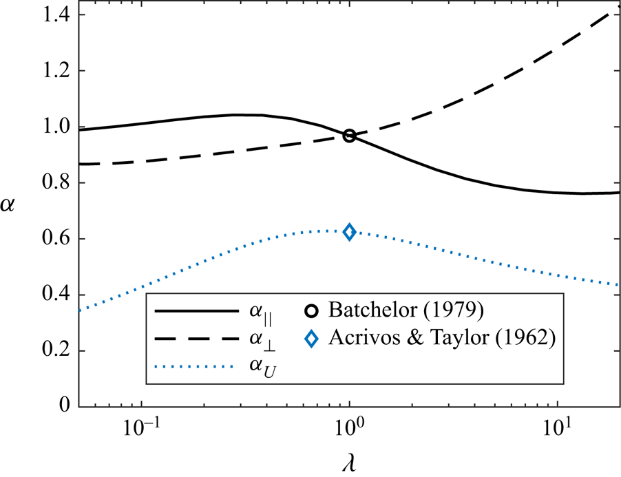
Figure 3. Variation in the mass transfer coefficient of a spheroid of varying aspect ratio but constant surface area in axisymmetric straining flow (black lines) and uniform flow (blue line). The black circle shows Batchelor's result for a sphere in axisymmetric strain (Batchelor Reference Batchelor1979), whilst the black diamond shows the equivalent result for a sphere in uniform flow (Acrivos & Taylor Reference Acrivos and Taylor1962).
The shape dependence for spheroids in axisymmetric strain may be contrasted to the shape dependence observed for axisymmetric, uniform flow around a fixed spheroid shown in figure 3 (Acrivos & Taylor Reference Acrivos and Taylor1962; Sehlin Reference Sehlin1969; Dehdashti & Masoud Reference Dehdashti and Masoud2020). Here, the surface flux exhibits the same scaling  ${Sh} = \alpha _U {Pe}_U^{1/3} + O(1)$, where ${Pe}_U=U_\infty ^* r/\kappa$ and $U_\infty ^*$ is the magnitude of the relative velocity (slip velocity) between the free stream and particle. Whilst it is of limited value to compare the absolute values of $\alpha$, some insight can be obtained by comparing the relative variation of each function. We observe that for a spherical particle with fixed translation velocity and surface area, flattening or elongating the particle results in a reduction in the surface flux. Likewise, for a spherical particle in rotation-dominated vortex stretching, flattening or elongating the particle also reduces the surface flux. However, in rotation-dominated vortex compression, flattening or elongating increases the surface flux. This observation is relevant to chain formation by marine diatoms, where each cell in a chain must experience an increased nutrient flux per unit area to benefit despite increased competition for nutrients by its neighbours (Pahlow et al. Reference Pahlow, Riebesell and Wolf-Gladrow1997).
One may also observe that rotation-dominated straining flow becomes considerably more effective than uniform flow at transferring solute from the particle surface at large aspect ratios. Of course, this result must depend upon the relative orientation of the free stream and particle axis, which is not varied here. Nonetheless, similar comparisons have found utility in determining when sinking or swimming may become a useful strategy for phytoplankton to increase their nutrient flux in turbulent water (Karp-Boss et al. Reference Karp-Boss, Boss and Jumars1996).
3.6. Further extensions
Two further generalisations of the surface coordinate system are to cases with non-zero body forces and torques. This would be necessary, for instance, to capture gyrotactic effects in the nutrient uptake of phytoplankton (Guasto et al. Reference Guasto, Rusconi and Stocker2012) or the behaviour of inertial particles. Such an extension can be accommodated by a suitable modification of the surface coordinate system, e.g. the inclusion of a body torque adds a skew–symmetric component to  $\boldsymbol{\Phi}$ in (3.15). However, in this case, one would also expect the orientation dynamics (and therefore the mean flow around the particle) to change, which would also affect the mean surface flux via the convection suppression effect.
4. Comparisons to numerical simulation
As a test of the results in in §§ 2 and 3, we conducted numerical simulations of the unsteady scalar transport around spheroids freely suspended in a linear shear. We describe our numerical methods in § 4.1 then examine two classes of arbitrary strain and rotational flows in § 4.2.
4.1. Methods
The unsteady convection diffusion equation (2.1) is solved using a second-order finite volume method, subject to the Dirichlet boundary condition  $\theta = 1$ on $S_p$ and the von-Neumann boundary condition on the outer boundary of the simulated domain. Equation (2.1) is discretised on a structured grid in prolate (4.1) or oblate (4.2) spheroidal coordinates $(\mu ,\theta ,\phi )$, depending upon the particle aspect ratio. The inner boundary $(\mu _0,\theta ,\phi )$ corresponds to the surface of the spheroid oriented in the Cartesian $x$ direction. The relative velocity field was evaluated in the body frame based on the coordinate of each cell centre using the expressions given by Kim & Karrila (Reference Kim and Karrila1991). The relative velocity field satisfies the impermeable, no slip boundary condition $\boldsymbol {u}=0$ on $S_p$.
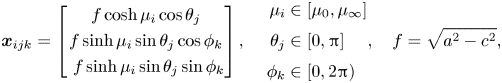 \begin{align} \boldsymbol{x}_{ijk} &= \begin{bmatrix} f\cosh\mu_i \cos\theta_j \\ f\sinh\mu_i \sin\theta_j \cos\phi_k \\ \,\,f\sinh\mu_i \sin\theta_j \sin\phi_k \end{bmatrix}, \quad \begin{aligned} \mu_i & \in [\mu_0, \mu_\infty] \\ \theta_j & \in [0, {\rm \pi}] \\ \phi_k & \in [0, 2{\rm \pi}) \\ \end{aligned}, \quad f = \sqrt{a^2-c^2}, \end{align}
 \begin{align} \boldsymbol{x}_{ijk} &= \begin{bmatrix} f\sinh\mu_i \sin \theta_j \\ f\cosh\mu_i \cos \theta_j \cos\phi_k \\ \,\,f\cosh\mu_i \cos \theta_j \sin\phi_k \end{bmatrix},\quad \begin{aligned} \mu_i & \in [\mu_0, \mu_\infty] \\ \theta_j & \in [-{\rm \pi}/2, {\rm \pi}/2] \\ \phi_k & \in [0, 2{\rm \pi}) \\ \end{aligned}, \quad f = \sqrt{c^2-a^2}. \end{align}
 The mesh resolution and spacing was chosen following the studies of Pahlow et al. (Reference Pahlow, Riebesell and Wolf-Gladrow1997) and Karp-Boss et al. (Reference Karp-Boss, Boss and Jumars1996). The mesh is discretised into  $150\times 64\times 64$ cells in the $(\mu ,\theta ,\phi )$ directions respectively, with uniform spacing in the $\theta$ and $\phi$ directions. Due to the nature of the spheroidal coordinate system chosen, the resolution varies across the surface of the particle and the outer boundary is very slightly oblate or prolate. The dimensions of the spheroid $a_i = (a,c,c)$ are chosen such that the surface area is $4{\rm \pi}$, equivalent in surface area to a sphere with unit radius. The outer boundary is chosen such that its largest dimension is $100$ and is very nearly spherical, having an aspect ratio between $0.999$ and $1.001$. To adequately resolve the thin concentration boundary layer, which is of thickness $\delta = {Pe}^{-1/3}$, we employ a mesh refinement in the $\mu$ direction such that the grid spacing is ${\rm \Delta} \mu _{i+1} = R {\rm \Delta} \mu _i$, where ${\rm \Delta} \mu _{i+1} = \mu _{i+1}-\mu _i$ is the spacing between adjacent cells in the $\mu$ direction. The initial spacing ${\rm \Delta} \mu _1$ is chosen such that the thickness of the largest cell near the particle surface is at most $2\times 10^{-4} \max (a,c)$ and the mesh refinement factor $R$ is chosen accordingly. For the most extreme aspect ratio $\lambda = 16$ ( $\lambda = 1/16$) at the largest Péclet number tested, this yields between $27$ (43) and $70$ (87) cells within a distance $\delta$ from the surface.
The solver is based on the scalarTransportFoam solver of OpenFOAM, which was modified to solve (2.1) for a time varying flow field. The convective term in (2.1) is discretised using a standard linear upwind Gaussian integration, and the diffusive term is discretised using a similar linear Gaussian scheme with an explicit non-orthogonal correction to maintain second-order accuracy. Time stepping is performed using an implicit Euler scheme and a time step of  ${\rm \Delta} t = 0.02$. Simulations were allowed sufficient time for the surface flux to reach a steady (or periodic) state. Where the particle motion is unsteady, the cycle average mass flux was evaluated over the interval $9T \le t < 10T$. Where the particle motion is steady, the steady state mass flux was evaluated at $t = 100$.
4.2. Results and discussion
In this section, we shall compare the results of our numerical simulations against the asymptotic results derived in § 2.
4.2.1. Pure strain
As our first test, we consider an arbitrary irrotational background velocity gradient  $\boldsymbol{\mathsf{G}}=\boldsymbol{\mathsf{E}}$. The particle motion in this case corresponds to case 1b of § 3.1 and the particle aligns itself with the most extensional (or compressive) direction of strain. Thus, the relative velocity gradient field is of the form
 \begin{equation} \boldsymbol{\mathsf{A}} = \begin{bmatrix} \sigma_1 & 0 & 0 \\ 0 & \sigma_2 & 0 \\ 0 & 0 & \sigma_3 \end{bmatrix}, \end{equation}
where  $\sigma _i$ are the eigenvalues of $\boldsymbol{\mathsf{E}}$. The topology of the relative flow field can therefore described by a single parameter $-1 \le s \le 1$ (Lund & Rogers Reference Lund and Rogers1994)
 \begin{equation} s = \frac{+3\sqrt{6} \sigma_1 \sigma_2 \sigma_3}{(\sigma_1^2 + \sigma_2^2 + \sigma_3^2)^{3/2}}. \end{equation}
When  $s = -1$, the background flow is an axisymmetric expansion; $s = 0$ corresponds to a 2-D strain and $s = 1$ corresponds to an axisymmetric contraction.
We computed the surface flux from prolate and oblate spheroids in an arbitrary straining flow over a range of  ${Pe}$. The result is shown in figure 4 for cases $\lambda = 4$ and $1/4$. For both prolate and oblate spheroids, there is a modest variation ( $15\,\%\text {--}30\,\%$) in the mass transfer coefficient as the strain topology is varied, which becomes more pronounced as the Péclet number is increased. In contrast, the mass transfer coefficient for a spherical body in a pure straining flow varies by less than $1\,\%$ over the same range of $s$ (Batchelor Reference Batchelor1979). When the Péclet number is large, the mass transfer rate approaches the limiting scaling ${Sh} = \alpha {Pe}^{1/3}$. The numerical coefficient $\alpha$ is well predicted by (2.24) and shows the correct qualitative dependence upon $s$. At ${Pe} = 10^4$, the discrepancy in the predicted mass transfer rate between theory and numerical simulations is within $2.5\,\%$ for the prolate case and within $3.1\,\%$ for the oblate case. This is partly due to the mesh refinement; additional tests at a higher resolution of $300 \times 128 \times 128$ suggest the numerical simulations slightly under-resolve the surface flux by around 2 % for the oblate case, which would improve the agreement seen here. Nonetheless, the leading order correction term to (2.24) is $O(1)$, which corresponds to a discrepancy in ${Sh}/{Pe}^{1/3}$ of $\sim 4.6\,\%$ at $Pe = 10^4$ and is comparable to the observed discrepancy.
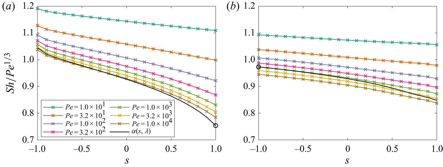
Figure 4. Mass transfer coefficient for (a) prolate  $\lambda =4$ and (b) oblate $\lambda =1/4$ spheroids in a pure straining flow, as a function of the strain topology parameter $s$. Coloured lines with markers show numerical simulations over ${Pe} = 10^1\text {--}10^4$. Black lines show the expected scaling coefficient $\alpha (s,\lambda )$ (2.24). Black circular markers show the axisymmetric result (3.25).
To examine the role of particle shape, we plot the scaling coefficient  $\alpha (s,\lambda )$ over a range of $s$ and $\lambda$ in figure 5. Markers show the value of ${Sh}/{Pe}^{1/3}$ from our numerical simulations at ${Pe}=10^4$ whilst the ruled surface shows the result of (2.24). We observe that prolate spheroids tend to experience a larger surface flux than oblate spheroids of equivalent surface area in the same flow. However, the trend is not always clear cut and is reversed for strain topologies near $s=1$, where spherical particles experience a larger surface flux.
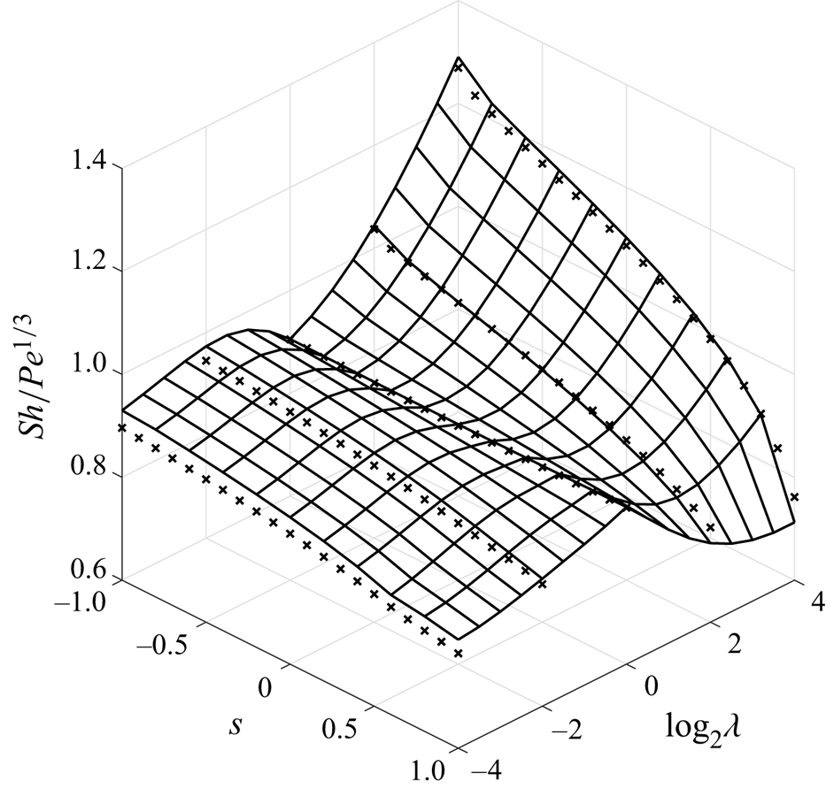
Figure 5. Mass transfer coefficient for spheroids in a pure straining flow, as a function of the strain topology parameter  $s$ and aspect ratio $\lambda$. The ruled surface shows the expected scaling coefficient $\alpha (s,\lambda )$ (2.24). Black markers show the result of numerical simulations conducted at ${Pe}=10^4$.
In figures 4 and 5, we observe that the surface flux is always larger in axisymmetric expansion ( $s=-1, -E_{11}/2 = E_{22} = E_{33} = 1/\sqrt {6}$) than axisymmetric contraction ( $s=+1, -E_{11}/2 = E_{22} = E_{33} = -1/\sqrt {6}$). This is remarkable, since both flows correspond to an axisymmetric strain; only the direction of the flow is reversed. At first glance, this appears to violate Brenner's flow reversal theorem (Brenner Reference Brenner1967; Vandadi, Jafari Kang & Masoud Reference Vandadi, Jafari Kang and Masoud2016; Masoud & Stone Reference Masoud and Stone2019), which states that for an isothermal body in steady flow, the surface flux is preserved under flow reversal $\boldsymbol {u} \rightarrow -\boldsymbol {u}$. However, we recall that the stable orientation of a free spheroid shifts under flow reversal. In this example, prolate spheroids align parallel to the Cartesian $1-$direction in axisymmetric contraction ( $s=+1, \sigma _1/2 = -\sigma _2 = -\sigma _3 = 1/\sqrt {6}$) and orthogonal to it in axisymmetric expansion ( $s=-1, \sigma _1 = \sigma _2 = -\sigma _3/2 = 1/\sqrt {6}$). The identities of $\sigma _1$ and $\sigma _3$ are reversed for oblate spheroids. This flow configuration is identical to the parallel and orthogonal flow configurations discussed in § 3.5 and shown in figure 3. Thus, the difference in the average transfer rate between $s=\pm 1$ is due to a change in the stable orientation of the spheroid.
4.2.2. Spinning and tumbling
As a numerical test of our result for spinning and tumbling spheroids, we consider a spheroid in a background velocity gradient  $\boldsymbol{\mathsf{G}}=\boldsymbol{\mathsf{E}}+\boldsymbol{\mathsf{W}}$ of the form
 \begin{equation} \boldsymbol{\mathsf{E}} = \frac{1}{\sqrt{6}} \begin{bmatrix} 2 & 0 & 0 \\ 0 & -1 & 0 \\ 0 & 0 & -1 \end{bmatrix}, \quad \boldsymbol{\mathsf{W}} = \begin{bmatrix} 0 & -\sin\theta_{\omega} & 0 \\ \sin\theta_{\omega} & 0 & -\cos\theta_{\omega} \\ 0 & \cos\theta_{\omega} & 0 \end{bmatrix}. \end{equation}
This corresponds to an axisymmetric straining flow with  $|\boldsymbol{\mathsf{E}}|=1$ and vorticity magnitude $|\boldsymbol{\omega}|=2$. By varying the angle $\theta _\omega$ between the background vorticity $\boldsymbol {\omega }$ and the $x_1$ axis, we survey different limiting behaviours of particle motion identified in § 3.1 and the relative flow field experienced by the particle depends upon is geometry. For example, a prolate particle will spin when $\theta _\omega = 0$ (case 2a) whereas it will tumble for $\theta _\omega = {\rm \pi}/2$ (case 2b). The situation is reversed for an oblate particle.
Figure 6 shows how the average mass transfer rate varies for prolate ( $\lambda = 4$) and oblate $(\lambda = 1/4)$ spheroids as the parameter $\theta _\omega$ is varied. The dependence is plotted as an implicit function of the axial strain rate $E_3$ (3.10) for ${Pe} = 10^1\text {--}10^4$. We first remark that as the Péclet number becomes large, the mass transfer rate approaches the scaling predicted by (3.25) and (2.24). As $\theta _\omega$ is varied, the particle motion switches from spinning to tumbling at $E_3 = 0$ and a pronounced change can be observed in the limiting mass transfer rate. There is a marked suppression of mass transfer near $E_3 = 0$ as the particle approaches the transition from spinning to tumbling. This is a demonstration of the suppression of convection by rotation first identified by Batchelor (Reference Batchelor1979). We note, however, that the presence of vorticity does not always suppress the convective transport. For instance, for the prolate spheroid in figure 6(a), tumbling induced by the vorticity component can enhance the convective transfer relative to the equivalent pure strain case (figure 4a).
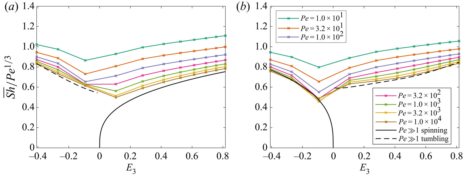
Figure 6. Average mass transfer coefficient for (a) prolate  $\lambda =4$ and (b) oblate $\lambda =1/4$ spheroids in an arbitrary shear (4.5a,b), as an implicit function of the mean axial strain rate $E_3$ (3.10). Coloured lines with markers show numerical simulations over ${Pe} = 10^1\text {--}10^4$. Black solid lines show the expected scaling coefficient for spinning motion (3.25). Black dashed lines show the expected scaling coefficient for tumbling motion (2.24).
Some remarks are in order. Firstly, the convection suppression/augmentation effect is essentially a hydrodynamic effect: it occurs as the result of the motion of a free spheroid and its alignment with the strain field. Secondly, this effect can be seen even at moderate Péclet number and becomes more pronounced as  ${Pe}$ increases. This underlines the observation that particle shape influences two factors in determining the mass transfer rate: it determines both the boundary condition for the scalar field and the behaviour of relative flow field.
5. Conclusion
In this paper, we have presented a general method to evaluate the average flux of solute from a rigid particle of arbitrary shape immersed in an arbitrary, open pathline flow. The main restrictions upon the shape of the particle are that it contains no sharp edges or regions of extreme curvature, where the thin boundary layer assumption breaks down. The flow may be steady or time periodic. When the flow is periodic, the average surface flux is equivalent to that of the same particle embedded in the mean flow field, provided the dimensionless period of the motion is  $T \ll {Pe}^{1/3}$. The Sherwood number scales as ${Pe}^{1/3}$, with a prefactor $\alpha$ which can be readily obtained through numerical integration once the particle geometry and surface flow field are specified.
We apply this result to compute the surface flux from a small, freely suspended spheroid in a steady linear shear. To do so, we compute the relative flow field experienced by the particle, which may be unsteady due to the particle motion. Through an analysis of Jeffery's equation, we identify four categories of motion: resting, spinning and 2-D or 3-D tumbling. The relative flow field is time periodic in the first three cases. In the spinning case, the average perceived flow field is an axisymmetric strain. In the 2-D tumbling case, the average flow field always corresponds to an equivalent spheroid in steady flow (resting). We provide a closed form expression (3.25) for the surface flux in the spinning case. We outline the numerical procedure to obtain the surface flux in the resting or 2-D tumbling cases. We also describe a simplification for the case of rotation-dominated flow  $|\boldsymbol {\omega }| \rightarrow \infty$. In this limit, there is a larger surface flux under vortex compression when compared to vortex stretching and this increase becomes significant for prolate bodies. These procedures may serve as the basis for analysing other, more complex geometries, or more complex rigid-body dynamics including inertia and gravity.
As a test of these analytical results, we have presented numerical simulations of the scalar transport and surface flux around spheroids in pure straining and a simplified shear flow. In all cases, we observe good agreement with the expected scaling law and mass transfer coefficient, up to the accuracy of the asymptotic approximation. In pure straining flows, the surface flux is steady and is prescribed by only three parameters: the Péclet number, the particle aspect ratio and a parameter describing the strain topology. In surveying this parameter space, we observe that prolate spheroids tend to experience a greater surface flux than oblate spheroids of equivalent surface area. When vorticity is present, we observe that the spinning or tumbling of the particle may suppress or augment the convective transfer, due to a realignment of the particle with respect to the average strain field. Two additional parameters are necessary to characterise the surface flux in all rotational flows and a complete survey of the parameter space is not practical. However, the space is sufficiently small that it may be readily tabulated for use as a model in a numerical simulation.
We anticipate that our results may find application in modelling the mass transfer from spheroidal or arbitrary particles in numerical simulations of particle laden flows, where models for the interphase mass transfer rate are required to take particle shape into account. Although the results presented here pertain to steady and time periodic flows, the results may serve in the same spirit in which steady flow mass transfer coefficients are employed to model the transfer rate in unsteady flows (Crowe et al. Reference Crowe, Schwarzkopf, Sommerfeld and Tsuji2012). Of particular interest is the mass transfer in turbulent environments, such as turbulent ocean waters home to planktonic osmotrophs (Karp-Boss et al. Reference Karp-Boss, Boss and Jumars1996) and microplastics (Law Reference Law2017). Here, the adaptation of shape to maximise surface flux may help explain the great diversity in the morphology of osmotrophs (Guasto et al. Reference Guasto, Rusconi and Stocker2012), or help identify which shapes of microplastics do the most harm. Another extension would be to include non-zero body torques or forces. This would allow, for instance, the consideration of gyrotactic effects in the motion of phytoplankton (Guasto et al. Reference Guasto, Rusconi and Stocker2012), or inertial effects in the rigid body dynamics of suspended particles.
Acknowledgements
The author acknowledges the use of the IRIDIS High Performance Computing Facility, and associated support services at the University of Southampton, in the completion of this work. Pertinent data for this paper are available at doi: 10.5258/SOTON/D1684.
Funding
This project has received funding from the European Union's Horizon 2020 research and innovation programme under the Marie Skłodowska-Curie grant agreement no. 846648.
Declaration of interest
The author reports no conflict of interest.


 Open access