


1. Introduction
Gravity-driven flows of one fluid over another can involve complex interactions between the two fluids, which can lead to a rich dynamical behaviour. Such flows occur in a wide range of natural and human-made systems, as in lava flow over less viscous lava (Balmforth et al. Reference Balmforth, Burbidge, Craster, Salzig and Shen2000; Griffiths Reference Griffiths2000), spreading of the lithosphere over the mid-mantle boundary (Lister & Kerr Reference Lister and Kerr1989; Dauck et al. Reference Dauck, Box, Gell, Neufeld and Lister2019), ice flow over an ocean (Kivelson et al. Reference Kivelson, Khurana, Russell, Volwerk, Walker and Zimmer2000; DeConto & Pollard Reference DeConto and Pollard2016) and over bedrock consisting of sediments and water (Fowler Reference Fowler1987; Stokes et al. Reference Stokes, Clark, Lian and Tulaczyk2007), flows in permeable rocks (Woods & Mason Reference Woods and Mason2000), liquid drops deforming over lubricated surfaces (Daniel et al. Reference Daniel, Timonen, Li, Velling and Aizenberg2017), and droplets motion on liquid-infused surfaces (Keiser et al. Reference Keiser, Keiser, Clanet and Quéré2017).
The flow of gravity currents (GCs) in circular geometry has been studied with a range of boundary conditions. In the absence of a lubricating layer, a common boundary condition along the base of a sole GC is no-slip. Such GCs of Newtonian fluids that are discharged at a rate proportional to  $t^{\alpha }$, where $t$ is time and $\alpha$ is a non-negative scalar, admit similarity solutions in which the front evolves proportionally to $t^{(3\alpha + 1)/8}$ (Huppert Reference Huppert1982). Similar axisymmetric GCs of power-law fluids having exponent $n$, where $n=1$ represents a Newtonian fluid and $n>1$ represents a strain-rate softening fluid, also admit similarity solutions in which the front propagation is proportional to $t^{[\alpha (2n+1) +1]/(5n+3)}$ (Sayag & Worster Reference Sayag and Worster2013).
On the other extreme, the presence of a lower fluid layer can significantly reduce friction at the base of the top fluid, resulting in extensionally dominated GCs. This is the case, for example, for ice shelves, which deform over the relatively inviscid oceans with weak friction along their interface. The late-time front evolution of such axisymmetric GCs of Newtonian fluids is proportional to  $t$ and is believed to be stable (Pegler & Worster Reference Pegler and Worster2012). However, when the top fluid is strain-rate softening, an initially axisymmetric front can become unstable and develop fingering patterns consisting of tongues separated by rifts (Sayag & Worster Reference Sayag and Worster2019).
In the more general case, friction along the base of GCs can vary spatiotemporally, as their stress field evolves. For example, the interface of an ice sheet with its underlying bedrock can consist of distributed melt water and sediments (e.g. Vogel et al. Reference Vogel, Tulaczyk, Kamb, Engelhardt, Carsey, Behar, Lane and Joughin2005). Subglacial sediments are believed to deform viscoplastically (Iverson, Hooyer & Baker Reference Iverson, Hooyer and Baker1998; Tulaczyk, Kamb & Engelhardt Reference Tulaczyk, Kamb and Engelhardt2000; Kamb Reference Kamb2001; Joughin, MacAyeal & Tulaczyk Reference Joughin, MacAyeal and Tulaczyk2004; Schoof Reference Schoof2004), and when saturated with water, the ice basal friction may be affected significantly by a complex subglacial hydrological network that can evolve in time (e.g. Nanni et al. Reference Nanni, Gimbert, Roux and Lecointre2021). Consequently, subglacial lubrication can collectively impose non-uniform and time-dependent friction along the ice base, and evolve spatiotemporally under the stresses imposed by the ice layer (Fowler Reference Fowler1981; Schoof & Hewitt Reference Schoof and Hewitt2013). This coupled ice–subglacial-water system may become unstable either over hard beds (Walder Reference Walder1982; Creyts & Schoof Reference Creyts and Schoof2009) or over sediment beds (Kyrke-Smith & Fowler Reference Kyrke-Smith and Fowler2014; Kasmalkar, Mantelli & Suckale Reference Kasmalkar, Mantelli and Suckale2019), and may contribute to the formation of complex flow patterns, such as ice streams and ice surges (Fowler Reference Fowler1987; Fowler & Johnson Reference Fowler and Johnson1995; Stokes et al. Reference Stokes, Clark, Lian and Tulaczyk2007; Sayag & Tziperman Reference Sayag and Tziperman2009; Kyrke-Smith, Katz & Fowler Reference Kyrke-Smith, Katz and Fowler2013). Such lubricated flows with spatiotemporally evolving friction were also modelled as two coupled GCs of Newtonian fluids spreading axisymmetrically one on top of the other (Kowal & Worster Reference Kowal and Worster2015). The early stage of these flows follows a similarity solution, in which the fronts of the two fluids evolve like  $t^{1/2}$, as in non-lubricated (no-slip) GCs (Huppert Reference Huppert1982), but they can have a radially non-monotonic thickness. Furthermore, laboratory experiments were found to be consistent with the similarity solutions after an initial transient state, but became unstable at a later stage, developing fingering patterns (Kowal & Worster Reference Kowal and Worster2015). It has been suggested that such instabilities appear when the jump in hydrostatic pressure gradient across the lubrication front is negative (Kowal & Worster Reference Kowal and Worster2019a,Reference Kowal and Worsterb).
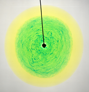
Despite the wide range of natural lubricated GCs that involve non-Newtonian fluids, the radial flow of a non-Newtonian fluid over a lubricated layer of Newtonian fluid has just recently been explored experimentally (Kumar et al. Reference Kumar, Zuri, Kogan, Gottlieb and Sayag2021). Motivated by glacier flow over lubricated bedrock, the experimental set-up consisted of a GC of a strain-rate softening fluid (xanthan gum solution) that has a power-law viscous deformation similar to ice (Glen Reference Glen1952), and a lubricating GC of a less viscous Newtonian fluid (diluted sugar solution). The pattern of both fluids in those constant flux  $(\alpha =1)$ experiments remained axisymmetric throughout the flow (figure 1), in contrast to the fingering patterns that emerged in the purely Newtonian experiments (Kowal & Worster Reference Kowal and Worster2015), as long as the flux ratio of the lubricating fluid to the non-Newtonian fluid was lower than ${\sim }0.06$. The fronts of the two fluids appeared to have a power-law time evolution with different exponents. In particular, the front of the top non-Newtonian fluid evolved with the same exponent $(2n+2)/(5n+3)$ as a non-lubricated power-law fluid (Sayag & Worster Reference Sayag and Worster2013), whereas the front of the Newtonian lubricating fluid evolved with an exponent $1/2$, similar to a Newtonian non-lubricated GC (Huppert Reference Huppert1982). Despite the similarity of the exponents with non-lubricated GCs, the fronts of those lubricated GCs evolved faster due to larger intercepts. In addition, in contrast with the monotonically declining thickness of non-lubricated GCs, the thickness of the lubricated, non-Newtonian fluid was found to be nearly uniform in the lubricated part of the flow, while that of the lubricating fluid was non-monotonic with localized spikes.

Figure 1. Snapshots from a laboratory experiment (Kumar et al. Reference Kumar, Zuri, Kogan, Gottlieb and Sayag2021) of a lubricated GC that consists of a strain-rate softening fluid (yellow) lubricated by a sugar solution (blue, appears green). The marked time at each snapshot is relative to the discharge initiation time  $t_L$ of the lubricating fluid.
Following up the experimental study of Kumar et al. (Reference Kumar, Zuri, Kogan, Gottlieb and Sayag2021), here we develop a theory for lubricated axisymmetric GCs of power-law fluids, and explore its major consequences. Specifically, we develop a mathematical model for axisymmetric flow of a viscous GC of a power-law fluid lubricated by a Newtonian GC, considering a general input flux of the form  $t^{\alpha }$, and show that in the general case, the flow has no global similarity solution of the first kind (§ 2). We then describe the numerical solver (§ 3), investigate several special cases that have similarity solutions (§ 4), and explore the possibility that the inner lubricating front outstrip the outer front (§ 5). Finally, we investigate the case of constant flux discharge (§ 6), compare our theoretical predictions with the laboratory experiments of Kumar et al. (Reference Kumar, Zuri, Kogan, Gottlieb and Sayag2021) (§ 7), and discuss caveats and implications (§ 8).
2. Mathematical model
Consider a power-law fluid having viscosity  $\mu$ and density $\rho$ that spreads axisymmetrically under its own weight over a horizontal rigid surface. Simultaneously, a lubricating film of Newtonian immiscible fluid of viscosity $\mu _\ell$ and density $\rho _\ell$ spreads axisymmetrically over the substrate and below the power-law fluid (figure 2). Both fluids are discharged at the origin of a cylindrical coordinate system in which $r$ is the radial coordinate and $z$ is the vertical coordinate. The upper and lower fluid fronts are denoted by $r_N(t)$ and $r_L(t)$ respectively, and the corresponding fluid thicknesses are denoted by $H(r,t)-h(r,t)$ and $h(r,t)$, respectively, where $t$ is the time variable. Beginning the discharge of the lubricating fluid at a time delay $t_L$, with respect to the upper fluid, creates two regions in the flow: an inner, lubricated region ( $r \leqslant r_L$) in which the power-law fluid flows at a finite velocity along the interface with the lubricating fluid, and an outer, non-lubricated region ( $r_L < r \leqslant r_N$) in which the power-law fluid meets the substrate and has zero velocity along it.

Figure 2. Diagram illustrating a GC of Newtonian fluid (blue) lubricating a GC of a power-law fluid (yellow). Exact solutions are singular at the origin, apart from the illustrated constant volume case  $\alpha =0$.
We assume that the radial extent of the flow is much greater than its thickness in both fluid layers, and that the flow is primarily radial. Together with the no-slip boundary condition along the substrate, this implies that the flow is shear-dominated in the non-lubricated region and in the lower fluid layer in the lubricated region. We also assume that the flow in the upper fluid layer in the lubricated region is shear-dominated due to back pressure applied by the non-lubricated layer downstream, which inhibits the growth of extensional stresses. We elaborate further on this assumption in § 8. Consequently, we apply the lubrication approximation in each fluid layer  $i$, with a dominant strain rate $\partial u_i / \partial z$, where $u_i(r,z,t)$ is the radial velocity component. Therefore, the axisymmetric Cauchy equations for each fluid layer, simplified for flows of low Reynolds numbers and lubrication approximations, are
 $$\begin{gather} \frac{\partial { p_i}}{\partial { r}}=\frac{\partial {}}{\partial { z}} \left( \mu_i\,\frac{\partial { u_i}}{\partial { z}} \right), \end{gather}$$
 $$\begin{gather}\frac{\partial { p_i}}{\partial { z}}={-}\rho_i g, \end{gather}$$
 $$\begin{gather}\frac{1}{r}\,\frac{\partial { (ru_i)}}{\partial { r}}+\frac{\partial { w_i}}{\partial { z}}=0, \end{gather}$$
to leading order, where  $w_i$ is the vertical velocity component, $p_i$ is the pressure field, and $g$ is the gravitational acceleration. The pressure is determined hydrostatically in (2.1b) because we assume a large Bond number, implying that the effects of surface tension are negligible compared to gravity. Since (2.1) satisfy the lubrication approximation, this model does not describe accurately the problem at early times, before the fluid radial extent is sufficiently greater than its thickness. We estimate the instant when lubrication approximation is first satisfied in § 7, where we compare the theoretical predictions with the experimental data.
The viscosity of the power-law fluid is determined by
 \begin{equation} \mu=k \left(\tfrac{1}{2} {\boldsymbol{\mathsf{E}}}:{\boldsymbol{\mathsf{E}}} \right)^{{{1}/{2}\left({{1}/{n}-1}\right)}}, \end{equation}
where  ${\boldsymbol{\mathsf{E}}}$ is the strain-rate tensor, $k$ is the consistency coefficient, and $n$ is the power-law exponent, which determines the fluid's response to stress. Specifically, $n=1$ represents a Newtonian fluid with dynamical viscosity $k$, with $n > 1$ a shear-thinning fluid, and $n < 1$ a shear-thickening fluid. In the lubrication limit, $\boldsymbol{\mathsf{E}}:\boldsymbol{\mathsf{E}} \approx (\partial u / \partial z)^{2}$ to leading order, so the viscosity of the power-law fluid simplifies to
 \begin{equation} \mu=k \left| \frac{1}{2}\,\frac{\partial u}{\partial z}\right|^{{{1}/{n}-1}}. \end{equation}
We assume that the total volumes of the power-law fluid and the Newtonian fluid evolve following a power law in time given by
 \begin{equation} 2 {\rm \pi}\int _{0} ^{r_N} (H-h)r \,{\rm d}r=Q t^{\alpha}, \end{equation}
and for  $t> t_L$,
 \begin{equation} 2 {\rm \pi}\int _{0} ^{r_L} hr \,{\rm d}r=Q_\ell\left(t-t_L\right)^{\alpha}, \end{equation}
where  $\alpha$ is a constant exponent, and $Q$ and $Q_\ell$ are constant coefficients representing, for instance, the discharge flux of each fluid when $\alpha =1$.
2.1. The non-lubricated region
In the non-lubricated region, the power-law fluid meets the substrate, and the lubricating fluid is absent. Integrating (2.1b), the pressure distribution is
 \begin{equation} p(z,r,t)=p_0+\rho g(H(r,t)-z), \end{equation}
where  $p_0$ is the ambient pressure over the top free surface of the power-law fluid. Integration of the radial force balance (2.1a) across the depth of the fluid layer, together with no-slip boundary conditions along the substrate and no stress along the free surface
 \begin{equation} u(z=0)=0, \quad \mu\,\frac{\partial u}{\partial z}(z=H)=0, \end{equation}
gives the radial velocity field
 \begin{equation} u(z,r,t)=2^{{{1-n}}}\left(\frac{\rho g}{k}\right) ^{{n}} \frac{\partial H}{\partial r} \left| \frac{\partial H}{\partial r} \right| ^{{n-1}} \frac{1}{1+n} \left[(H-z)^{{n+1}}-H^{{n+1}}\right]. \end{equation}
Similar integration of the continuity equation (2.1c), accounting for a free surface at the upper boundary  $z=H(r,t)$, and assuming no normal flow through the substrate, gives the Reynolds equation
 \begin{equation} \frac{\partial { H}}{\partial { t}}+\frac{1}{r}\,\frac{\partial {(rq)}}{\partial { r}}=0, \end{equation}
which should satisfy the boundary conditions
 \begin{equation} H(r=r_N)=0 \quad \textrm{and} \quad q(r=r_N)=0, \end{equation}
where the local flux  $q$ is determined using (2.7) to give
 \begin{equation} q=\int ^{H} _{0} u\,{\rm d}z={-}2^{1-n}\left(\frac{\rho g}{k}\right)^{{n}}\frac{\partial { H}}{\partial { r}}\left|\frac{\partial { H}}{\partial { r}} \right|^{{n-1}}\frac{1}{n+2}\,H^{{n+2}}. \end{equation}
2.2. The lubricated region
As in the non-lubricated region and assuming continuity of pressure at the fluid–fluid interface  $z=h$, the pressure in the lubricated region is determined hydrostatically by
 $$\begin{gather} p(z)=p_0+\rho g(H-z),\quad \textrm{where} \ h \leqslant z \leqslant H, \end{gather}$$
 $$\begin{gather}p_\ell (z)=p_0+\rho g(H-h)+\rho _\ell g(h-z), \quad \textrm{where} \ 0 \leqslant z \leqslant h. \end{gather}$$
The radial force balances simplify to
 $$\begin{gather} \frac{k}{2^{{{1}/{n}-1}}}\,\frac{\partial}{\partial z}\left( \frac{\partial u}{\partial z}\left| \frac{\partial u}{\partial z}\right| ^{{{1}/{n}-1}} \right)= \frac{\partial p}{\partial r}, \quad \textrm{where} \ h \leqslant z \leqslant H, \end{gather}$$
 $$\begin{gather}\mu _\ell\,\frac{\partial ^{2} u_\ell}{\partial z^{2}}= \frac{\partial p_\ell}{\partial r}, \quad \textrm{where} \ 0 \leqslant z \leqslant h, \end{gather}$$
together with the boundary conditions
 $$\begin{gather} u_\ell=0, \quad \textrm{where} \ z=0, \end{gather}$$
 $$\begin{gather}u_\ell=u, \quad k\left|\frac{1}{2}\,\frac{\partial { u}}{\partial { z}}\right| ^{{{1}/{n}-1}}\frac{\partial { u}}{\partial { z}}=\mu _\ell\, \frac{\partial u_\ell}{\partial z}, \quad \textrm{where} \ z=h, \end{gather}$$
 $$\begin{gather}\frac{\partial u}{\partial z}=0, \quad \textrm{where} \ z=H, \end{gather}$$
which represent, respectively, no-slip along the solid substrate, continuous flow velocity and shear stress at the fluid–fluid interface, and no shear stress along the free surface of the power-law fluid. Integrating the radial force balance (2.12) across the thickness of each fluid layer, and using the boundary conditions (2.13), we get the radial velocity fields in each fluid layer:
 \begin{align} u(z,r,t)&= 2^{1-n}\left(\frac{\rho g}{k}\right)^{{n}}\frac{1}{1+n}\,\frac{\partial H}{\partial r} \left| \frac{\partial H}{\partial r}\right|^{n-1} \left[(H-z)^{{1+n}}-(H-h)^{{1+n}}\right]\nonumber\\ &\quad -\frac{\rho g}{\mu _\ell}\left[\frac{\partial H}{\partial r}\left(Hh-\frac{h^{2}}{2}\right)+\frac{h^{2}}{2}\,\frac{\rho _\ell -\rho}{\rho}\,\frac{\partial h}{\partial r}\right], \end{align}
 \begin{align} u_\ell(z,r,t)&={-}\frac{\rho g}{\mu _\ell}\left[\frac{\partial H}{\partial r}\left(Hz-\frac{z^{2}}{2}\right)+\frac{1}{2}\,\frac{\rho _\ell -\rho}{\rho}\,\frac{\partial h}{\partial r}\left(2hz-z^{2}\right)\right]. \end{align}
The Reynolds equations corresponding to each fluid layer have forms similar to those of the non-lubricated region,
 $$\begin{gather} \frac{\partial h}{\partial t}+\frac{1}{r}\,\frac{\partial (rq_\ell)}{\partial r}=0, \end{gather}$$
 $$\begin{gather}\frac{\partial (H-h)}{\partial t}+\frac{1}{r}\,\frac{\partial (rq)}{\partial r}=0, \end{gather}$$
and should satisfy the boundary conditions
 \begin{equation} h=0, \quad q_\ell=0 \quad \textrm{at} \ r=r_L,\\ \end{equation}
and
 \begin{equation} q^{+}=q^{-}, \quad H^{+}=H^{-} \quad \textrm{at} \ r=r_L,\end{equation}
where (2.16b) signifies flux and height continuity across  $r_L$. The local fluxes result from integrating (2.14) to get
 \begin{align} q=\int_h ^{H} u\,{\rm d}z &={-}2^{1-n}\left(\frac{\rho g}{k}\right)^{{n}} \frac{\partial H}{\partial r} \left| \frac{\partial H}{\partial r}\right|^{{n-1}}\frac{1}{n+2}\,(H-h)^{{n+2}}\nonumber\\ &\quad -(H-h)\,\frac{h \rho g}{\mu _\ell}\left[\frac{\partial H}{\partial r}\,(H-h)+\frac{h}{2}\left(\frac{\partial H}{\partial r}+\frac{\rho _\ell-\rho}{\rho}\,\frac{\partial h}{\partial r}\right)\right], \end{align}
 \begin{align} q_\ell&=\int_0 ^{h} u_\ell\,{\rm d}z ={-}\frac{h^{2}}{2}\,\frac{\rho g}{\mu _\ell}\left[\frac{\partial H}{\partial r}\,(H-h)+\frac{2h}{3}\left(\frac{\partial H}{\partial r}+\frac{\rho _\ell-\rho}{\rho}\,\frac{\partial h}{\partial r}\right)\right].\end{align}
We note that without a lubricant, this set of partial differential equations (PDEs) is reduced to that of the non-lubricated region, which is consistent with the non-lubricated power-law GC model (Sayag & Worster Reference Sayag and Worster2013), and particularly with the Newtonian non-lubricated GC when  $n=1$ (Huppert Reference Huppert1982). In addition, the full PDE set for the Newtonian case ( $n=1$) and constant source fluxes ( $\alpha =1$) is consistent with the model for Newtonian lubricated GCs (Kowal & Worster Reference Kowal and Worster2015).
2.3. Dimensionless equations
We non-dimensionalize equations (2.4), (2.8)–(2.10) and (2.15)–(2.17) with the following time, length and height scales:
 $$\begin{gather} t \equiv \mathcal{T}\,\hat{t}, \end{gather}$$
 $$\begin{gather}r \equiv \left( \left(\frac{\rho g}{k}\right)^{n} Q^{2n+1} \mathcal{T}^{\alpha(1+2n)+1} \right)^{{{1}/({5n+3})}} \hat{r}, \end{gather}$$
 $$\begin{gather}(H,h)\equiv \left( \left(\frac{\rho g}{k}\right)^{{-}2n} Q^{1+n} \mathcal{T}^{\alpha(1+n)-2} \right)^{{{1}/({5n+3})}} (\hat{H},\hat{h}), \end{gather}$$
where hats denote dimensionless quantities. The resulting dimensionless model, dropping hats, in the non-lubricated region  $r_L \leqslant r \leqslant r_N$ is
 \begin{equation} \frac{\partial H}{\partial t}+\frac{1}{r}\,\frac{\partial (rq)}{\partial r}=0, \end{equation}
where
 \begin{equation} q={-}\mathscr{N}\,\frac{\partial H}{\partial r}\left|\frac{\partial H}{\partial r} \right|^{{n-1}}H^{n+2},\quad \mathscr{N}=\frac{2^{{1-n}}}{n+2}, \end{equation}
and in the lubricated region  $0 \leqslant r \leqslant r_L$ it is
 $$\begin{gather} \frac{\partial h}{\partial t}+\frac{1}{r}\,\frac{\partial (rq_\ell)}{\partial r}=0, \end{gather}$$
 $$\begin{gather}\frac{\partial (H-h)}{\partial t}+\frac{1}{r}\,\frac{\partial (rq)}{\partial r}=0, \end{gather}$$
where
 \begin{align} q&={-} \mathscr{N}\,\frac{\partial H}{\partial r} \left| \frac{\partial H}{\partial r}\right|^{n-1}(H-h)^{2+n}\nonumber\\ &\quad - \mathscr{M} h(H-h) \left[\frac{\partial H}{\partial r}\,(H-h)+\left(\frac{\partial H}{\partial r}+\mathscr{D}\,\frac{\partial h}{\partial r}\right)\frac{h}{2}\right], \end{align}
 \begin{align} q_\ell&={-}\mathscr{M}\,\frac{h^{2}}{2}\left[\frac{\partial H}{\partial r}\,(H-h)+\frac{2h}{3}\left(\frac{\partial H}{\partial r}+\mathscr{D}\,\frac{\partial h}{\partial r}\right)\right], \end{align}
and where the boundary conditions are
 $$\begin{gather} q=0, \quad H=0 \quad \textrm{at}\ r=r_N, \end{gather}$$
 $$\begin{gather}q_\ell=0, \quad h=0, \quad q^{+}=q^{-}, \quad H^{+}=H^{-} \quad \textrm{at}\ r=r_L, \end{gather}$$
 $$\begin{gather}\lim_{r\rightarrow 0} (2{\rm \pi} rq)=\alpha t^{\alpha -1}, \quad \textrm{and for }t>t_L\quad \lim_{r\rightarrow 0} (2{\rm \pi} rq_\ell)=\alpha \mathscr{Q}\left(t-t_L\right)^{\alpha -1}, \end{gather}$$
and the total instantaneous volumes of the power-law and Newtonian fluids are
 \begin{equation} 2 {\rm \pi}\int _{0} ^{r_N} (H-h)r \,{\rm d}r=t^{\alpha}, \end{equation}
and for  $t>t_L$
 \begin{equation} 2 {\rm \pi}\int _{0} ^{r_L} hr \,{\rm d}r=\left(t-t_L\right)^{\alpha}, \end{equation}
respectively. The resulting dimensionless quantities
 \begin{equation} \left.\begin{gathered} \mathscr{Q}\equiv\frac{Q_\ell}{Q},\quad \mathscr{D}\equiv\frac{\rho _\ell-\rho}{\rho},\quad n,\quad \alpha,\\ \mathscr{M}\equiv\frac{\mu}{\mu_\ell}= \frac{\rho g}{\mu_\ell}\left(\frac{k}{\rho g}\right)^{{{8n}/({5n+3})}} \left(\frac{\mathcal{T}^{5-\alpha}}{Q}\right)^{{({n-1})/({5n+3})}}, \end{gathered}\right\} \end{equation}
represent respectively the discharge flux ratio, the relative density difference of the lubricating and power-law fluids, the power-law fluid exponent, the volume growth exponent, and the dynamic viscosity ratio.
The scale for the non-Newtonian fluid viscosity is based on the leading-order viscosity (2.3) and the spatial scales in (2.18). Specifically, we evaluate the characteristic scale for the strain rate  $\partial u/\partial z$ in (2.3) using (2.7) to get $[\partial {u}/\partial {z}]\propto ({\rho g}/{k})^{n}{H^{2n}}/{R^{n}}$. Substituting the scales (2.18b,c) in the strain rate, we find that the characteristic viscosity scale is $[\mu ]\sim \rho g({k}/{\rho g})^{8n/(5n+3)}({\mathcal {T}^{5-\alpha }}/{Q})^{(n-1)/(5n+3)}$, which depends on the time scale $\mathcal {T}$. That time scale, which also enters the viscosity ratio $\mathscr {M}$ (see (2.25e)), is scaled out of the equations in the two special cases $n=1$ and $\alpha =5$. Therefore, in the late-time limit ( $t/t_L\gg 1$), the system no longer depends on the time scale $t_L$, and admits a global similarity solution of the first kind in these two special cases. For any other values of $n$ and $\alpha$, including the constant flux case ( $\alpha =1$), such global similarity solutions do not exist. Nevertheless, as we show in § 4, we find several additional asymptotic limits in which part of the flow evolves in a self-similar manner.
In the general case  $n\ne 1$ and $\alpha \ne 5$, there are enough relations to determine the time scale $\mathcal {T}$ (see (2.18)) independently of the height and radial scales. Specifically, requiring that the scales of the two contributions to the flux in the top fluid layer (2.22a) balance leads to the relation $\mathscr {M}(\mathcal {T})=\mathscr {N}$ that can be solved for the time scale $\mathcal {T}$, which upon substitution in (2.18) leads to independent radial scale $\mathcal {R}$ and thickness scale $\mathcal {H}$, given by
 $$\begin{gather} \mathcal{T}^{(1-n)(\alpha-5)}=Q^{n-1}\left(\mathscr{N}\,\frac{\mu_\ell}{\rho g}\right)^{5n+3} \left(\frac{\rho g}{k}\right) ^{8n}, \end{gather}$$
 $$\begin{gather}\mathcal{R}^{(1-n)(\alpha-5)}=Q^{2(n-1)}\left(\mathscr{N}\,\frac{\mu_\ell}{\rho g}\right)^{\alpha+1+2\alpha n} \left(\frac{\rho g}{k}\right)^{n(3\alpha+1)}, \end{gather}$$
 $$\begin{gather}\mathcal{H}^{(1-n)(\alpha-5)}=Q^{n-1}\left(\mathscr{N}\,\frac{\mu_\ell}{\rho g}\right)^{\alpha-2+\alpha n} \left(\frac{\rho g}{k}\right) ^{2n(\alpha-1)}. \end{gather}$$
Therefore, in the more general case ( $n\ne 1$ and $\alpha \ne 5$), which does not admit global similarity solution of the first kind, the above may represent the time, radius and thickness scales. The time scale $\mathcal {T}$ can also be set by the lubricating fluid discharge time $t_L$, as we do when comparing the theoretical predictions to the experimental measurements in § 7.
3. Numerical solutions
We solve the dimensionless model (2.19)–(2.25a–e) numerically explicitly using the Matlab PDEPE solver, with an open-ended, non-uniform and time-dependent adaptive spatial mesh, and using the dimensional  $t_L$ as the time scale $\mathcal {T}$, so that $\hat {t}_L=1$. We find that lower spatial resolution can be used in most of the domain if the mesh is spaced logarithmically, and is denser around the fluid fronts, where the fluid heights drop sharply and the slopes $\partial { H}/\partial { r}$ and $\partial { h}/\partial { r}$ become singular. Therefore, we use a non-uniform spatial mesh that consists of two Gaussian distributions centred at the fronts $r_N$ and $r_L$, and uniform distributions between the origin and $r_L$, the two fronts, and beyond $r_N$ (figure 3). The instantaneous front positions $r_N(t)$ and $r_L(t)$ are determined where $H(r,t) \leqslant 10^{-6}$ and $h(r,t) \leqslant 10^{-6}$, respectively. Since the fronts evolve, we divide the simulation time into a set of intervals, and over each interval, we solve the PDE system and then adapt the spatial mesh. The mesh adaptation is done by predicting the front positions in the next time interval using the recent solution and the front evolution equations
 \begin{equation} \dot{r}_{N}(t)=\lim _{r\rightarrow r_{N}} \frac{q}{H} \quad \textrm{and} \quad \dot{r}_{L}(t)=\lim _{r\rightarrow r_{L}} \frac{q_{\ell}}{h}. \end{equation}
This technique allows us to keep higher mesh density centred at the front positions, where variations in the fields are larger, and lower density elsewhere, where variations are milder.

Figure 3. (a) Mesh density and (b) a solution at time  $t/t_L=100$, showing the lubricated fluid (thick) and the lubricating fluid (thin) for $n=1$, $\alpha =1$, $\mathscr {M}=1$, $\mathscr {Q}=0.2$ and $\mathscr {D}=0.1$. Front positions (red circles) are determined where each fluid thickness drops below $10^{-6}$. Substrate is not pre-wetted ahead of the intrusion, and each fluid thickness ahead of its front diminishes rapidly to zero.
We validated our numerical solver using several known asymptotic solutions. In the limit  $\mathscr {Q}=0$ (no lubricating fluid), our model converges to a GC that propagates under a no-slip condition along the substrate, which has a similarity solution $r_N(t) \propto t^{[\alpha (2n+1)+1]/{(5n+3)}}$ (Huppert Reference Huppert1982; Sayag & Worster Reference Sayag and Worster2013). We find that our numerical solutions for the fluid heights and for the leading front are consistent with those theoretical predictions (Appendix A). In particular, the discrepancy between the predicted and computed exponents is less than $5\times 10^{-3}$ and can be minimized further with a higher spatial resolution. In the limit $n=1$ and $\alpha =1$, our model converges to a purely Newtonian lubricated GC released at constant flux, which has a similarity solution $r_L,r_N\propto t^{1/2}$ (Kowal & Worster Reference Kowal and Worster2015). We find that our numerical solutions are consistent with both the front and thickness predictions for a wide range of $\mathscr {M}$ and $\mathscr {Q}$ values (Appendix A).
4. Similarity solutions
The model described by (2.19)–(2.25) admits similarity solutions in several special cases. Specifically, global similarity solutions exist when the top fluid is also Newtonian ( $n=1$), or when the mass-discharge exponent is $\alpha =5$. In addition, part of the flow evolves in a self-similar manner in the asymptotic limits of the viscosity ratio $\mathscr {M}$. Finally, for any parameter combination, the solutions in the vicinity of each front evolve in a self-similar manner.
4.1. The similarity solution for Newtonian fluids ( $n=1$)

When the top fluid is Newtonian ( $n=1$), the viscosity ratio $\mathscr {M}$ is independent of $\mathcal {T}$, and the resulting purely Newtonian coupled flow admits a global similarity solution. This case, restricted to a constant flux ( $\alpha =1$), has been explored thoroughly (Kowal & Worster Reference Kowal and Worster2015). For the general case of $\alpha \geqslant 0$, the PDE set can be reduced to an ordinary differential equation set with similarity variable
 \begin{equation} \eta=\frac{r}{t^{({3\alpha +1})/{8}}}\left(\frac{\rho g}{k}\,Q^{3}\right)^{-{1}/{8}}, \end{equation}
and a solution of the form
 \begin{equation} \left(H,h\right)=t^{({\alpha-1})/{4}}\left(Q\,\frac{k}{\rho g}\right)^{{1}/{4}}\left(F,f\right), \end{equation}
where  $F$ and $f$ are dimensionless functions of $\eta$. Therefore, the fronts of both the lubricated and lubricating fluids evolve like
 \begin{equation} \left(r_N,r_L\right)=\left(\eta_N,\eta_L\right)t^{({3\alpha+1})/{8}} \left( Q^{3} \frac{\rho g}{k} \right)^{{1}/{8}}, \end{equation}
where  $\eta _N\equiv \eta (r=r_N)$ and $\eta _L\equiv \eta (r=r_L)$ are numerical coefficients of order $1$. These solutions have structure identical to that of the classical solution for Newtonian GCs (Huppert Reference Huppert1982). Upon substitution, the Reynolds equations (2.8) and (2.15) become, for the non-lubricated region ( $\eta _L\leqslant \eta \leqslant \eta _N$),
 \begin{equation} \left(\frac{\alpha-1}{4}\right)F-\left(\frac{3\alpha+1}{8}\right)\eta F'=\frac{1}{3\eta}(\eta F'F^{3})', \end{equation}
where prime denotes a derivative with respect to  $\eta$, and for the lubricated region ( $0\leqslant \eta \leqslant \eta _L$),
 $$\begin{gather} \left(\frac{\alpha-1}{4}\right)\left(F-f\right)-\left(\frac{3\alpha+1}{8}\right)\eta\left(F'-f'\right) +\frac{1}{\eta}\left(\eta q\right)'=0, \end{gather}$$
 $$\begin{gather}\left(\frac{\alpha-1}{4}\right)f-\left(\frac{3\alpha+1}{8}\right)\eta f' +\frac{1}{\eta}\left(\eta q_\ell\right)'=0, \end{gather}$$
where
 $$\begin{gather} q ={-}\tfrac{1}{3}F'(F-f)^{3}-\mathscr{M}f(F-f)[F'(F-f)+\tfrac{1}{2}\,f(\mathscr{D}f'+F')], \end{gather}$$
 $$\begin{gather}q_\ell={-}\mathscr{M}{f^{2}}[\tfrac{1}{2}\,F'(F-f)+\tfrac{1}{3}\,f(\mathscr{D}f'+F')]. \end{gather}$$
The corresponding boundary conditions (2.23) become
 $$\begin{gather} F=0, \quad q=0 \quad \textrm{at}\ \eta=\eta_N, \end{gather}$$
 $$\begin{gather}f=0, \quad q_\ell=0, \quad F^{+}=F^{-}, \quad q^{+}=q^{-} \quad \textrm{at}\ \eta=\eta_L, \end{gather}$$
 $$\begin{gather}\lim _{\eta \rightarrow 0} 2 {\rm \pi}\eta q = \alpha, \quad \lim _{\eta \rightarrow 0} 2 {\rm \pi}\eta q_\ell = \alpha \mathscr{Q}, \end{gather}$$
where the last condition implies convergence to a similarity solution a long time after the initiation of the fluid discharge,  $t \gg t_L$.
For  $\alpha =1$, the model converges to that of Kowal & Worster (Reference Kowal and Worster2015), and the similarity solutions that we predict for general $\alpha$ are consistent with our full numerical solution (figures 4 and 5).

Figure 4. (a) The numerical solutions for the evolution of the dimensionless fronts for  $\alpha =1,2,3,4,5$, $n=1$ and for $\alpha =5$, $n=1.25$ (coloured lines and dashed lines) for $\mathscr {Q}=0.2$, $\mathscr {D}=0.1$ and $\mathscr {M}=100$. Regression to the late-time solutions ( $t/t_L>10$) to power-law evolution along one decade of time (dash, black) results in exponents (values in colour) consistent with the global similarity for the $n=1$ cases ( $t^{(3\alpha +1)/8}$, (4.2b)) and with the $\alpha =5$ cases ( $t^{2}$, (4.8b)). The inset shows the computed intercepts $\eta _N(\diamond ),\eta _L({\square })$ versus $\alpha$. (b) The normalized thicknesses $H/t,h/t$ along the normalized radius $r/t^{2}$ at selected dimensionless time $t/t_L$ when $\alpha =5$ and $n=1$. This shows the relatively rapid convergence of the numerical solution to an asymptotic similarity solution (4.8), where the front positions at the late-time instant $t/t_L=97.9$ are $\eta _N\approx 0.621$, $\eta _L\approx 0.473$, correspondingly with the computed values in the inset of (a).

Figure 5. The asymptotic solutions in the vicinity of the fronts  $F(\eta ),f(\eta )$ (see (4.18a,b), (4.21)) given by the non-lubricated GC similarity solutions (blue dotted lines), compared with the full numerical solutions of lubricated GCs (solid lines) for $\mathscr {M}=100$, $\mathscr {Q}=0.1$, $\mathscr {D}=1$, $\alpha =1$ and $n=0.5,1,2$ at $t/t_L\approx 20$. The positions of the fronts predicted by the non-lubricated GC solutions are cyan $\bigtriangledown$ ( $\eta _N$) and cyan $\Diamond$ ( $\eta _L$), but to have the shapes of the two solutions more clearly compared, we translated the asymptotic solutions so that their fronts coincide with those of the lubricated GC solution ( ${\square }, \circ, {\triangle }$ markers). Each inset zooms into the region near the lubricating fluid front marked by a rectangle.
4.2. The similarity solution for mass-discharge exponent $\alpha = 5$

When the top fluid is non-Newtonian,  $n\neq 1$, the viscosity ratio $\mathscr {M}$ becomes independent of the time scale $\mathcal {T}$ for a discharge exponent $\alpha =5$, and the resulting flow also admits a similarity solution with similarity variable
 \begin{equation} \eta =\frac{r}{t^{2}} \left[ Q^{2n+1} \left(\frac{\rho g}{k}\right)^{n} \right]^{{-1}/{(5n+3)}}, \end{equation}
and a solution of the form
 \begin{equation} (H,h)= t\left[Q^{1+n} \left(\frac{k}{\rho g}\right)^{2n} \right]^{{1}/{(5n+3)}} (F,f), \end{equation}
where  $F$ and $f$ are dimensionless functions of $\eta$. Therefore, the fronts of both the lubricated and lubricating fluids evolve like
 \begin{equation} \left(r_N,r_L\right)=\left(\eta_N,\eta_L\right)t^{2} \left[ Q^{2n+1} \left(\frac{\rho g}{k}\right)^{n} \right]^{{1}/{(5n+3)}}, \end{equation}
where  $\eta _N$ and $\eta _L$ are numerical coefficients of order $1$. Upon substitution, the Reynolds equations (2.8) and (2.15) become, for the non-lubricated region ( $\eta _L\leqslant \eta \leqslant \eta _N$)
 \begin{equation} F-2F'\eta=\mathscr{N}\,\frac{1}{\eta} (\eta F' \left|F'\right|^{{n-1}}F^{{n+2}} )', \end{equation}
and for the lubricated region ( $0\leqslant \eta \leqslant \eta _L$)
 $$\begin{gather} \left(F-f\right)-2(F'-f')\eta+\frac{1}{\eta}\left(\eta q \right)'=0, \end{gather}$$
 $$\begin{gather}f-2f'\eta+\frac{1}{\eta}\left(\eta q_\ell \right)'=0, \end{gather}$$
where
 $$\begin{gather} q={-}\mathscr{N}F' \left|F'\right|^{n-1}\left(F-f\right)^{n+2}-\mathscr{M} f (F-f) \left[ F'(F-f)+\tfrac{1}{2}\,f (\mathscr{D}f'+F') \right], \end{gather}$$
 $$\begin{gather}q_\ell={-}\mathscr{M}{f^{2} }\left[\tfrac{1}{2}F'(F-f)+\tfrac{1}{3}\,f (F'+\mathscr{D}f') \right]. \end{gather}$$
The corresponding boundary conditions (2.23) become
 $$\begin{gather} F=0, \quad q=0 \quad \textrm{at} \ \eta=\eta_N, \end{gather}$$
 $$\begin{gather}f=0, \quad q_\ell=0, \quad F^{+}=F^{-}, \quad q^{+}=q^{-} \quad \textrm{at}\ \eta=\eta_L, \end{gather}$$
 $$\begin{gather}\lim _{\eta \rightarrow 0} 2 {\rm \pi}\eta q = 5, \quad \lim _{\eta \rightarrow 0} 2 {\rm \pi}\eta q_\ell = 5 \mathscr{Q}. \end{gather}$$
 Figure 4 shows the numerical solution of the full PDE set for  $\alpha =5$ for varying power-law exponent values. We find that the numerical solutions are consistent with the predicted similarity solution (4.8). This consistency validates further the numerical simulation for the combination of lubricated GCs with lubricated power-law fluid.
We note that a similarity solution at  $\alpha =5$ arises also in other GCs with radial symmetry, but of different settings. We elaborate on this aspect in § 8.
4.3. Similarity solutions for the asymptotic limits in $\mathscr {M}$: the upper fluid solid and liquid limits

In the general case of  $\alpha \neq 5$ and $n \neq 1$, our model does not admit global similarity solutions of the first kind. However, a similarity solution arises in part of the flow domain in each of the asymptotic limits of the viscosity ratio, in which the upper fluid layer is either relatively more viscous ( $\mathscr {M} \gg 1$, the ‘solid’ limit) or relatively less viscous ( $\mathscr {M} \ll 1$, the ‘liquid’ limit) compared with the lower fluid layer.
4.3.1. The top layer solid limit, $\mathscr {M} \gg 1$

The limit  $\mathscr {M} \gg 1$ represents the case where the top fluid is much more viscous than the lubricating fluid. One motivation to study this limit is the geophysical setting of ice sheets creeping over less viscous lubricated beds. In this case, the leading-order scaling of the power-law fluid local flux in the lubricated region (2.22a) is
 \begin{equation} q \approx{-} \mathscr{M}h(H-h)\left[\frac{\partial { H}}{\partial {r}}\,(H-h)+\left(\frac{\partial { H}}{\partial {r}}+\mathscr{D}\,\frac{\partial { h}}{\partial {r}}\right)\frac{h}{2}\right], \end{equation}
which is identical to the scaling of the Newtonian lubricating fluid flux (2.22b). In such a case, the three scales  $\mathcal {H}$, $\mathcal {R}$ and $\mathcal {T}$ in the lubricated region cannot be determined independently despite the fact that the upper fluid is a power-law fluid. Therefore, both fluids in the lubricated region have a similarity solution in which the dimensionless front in the lubricated region evolves with an $n$-independent exponent
 \begin{equation} r_L=\eta_L t^{({3\alpha+1})/{8}}, \end{equation}
where the intercept  $\eta _L$ may depend on the system dimensionless numbers. The exponent in (4.14) is consistent with the predictions made for the special cases discussed above. Specifically, for $n=1$ it is $(3\alpha +1)/8$ as we predict in (4.2b), and for $\alpha =5$ it is $2$ independently of $n$ as we predict in (4.8b). This similarity solution does not reveal the evolution of the fluid front $r_N$ in the non-lubricated region, which depends on the fluid exponent $n$.
$n$.
4.3.2. The top layer ‘liquid’ limit, $\mathscr {M} \ll 1$

The second asymptotic limit,  $\mathscr {M} \ll 1$, in which the top fluid is much less viscous than the underlying fluid, also admits a similarity solution, but of a different subset of the model. In this case, the leading-order scaling of the power-law fluid local flux in the lubricated region (2.22a) is
 \begin{equation} q \approx{-} \mathscr{N}\,\frac{\partial H}{\partial r} \left| \frac{\partial H}{\partial r}\right|^{{n-1}}(H-h)^{{2+n}}, \end{equation}
which is identical to the scaling of the power-law fluid in the non-lubricated region (2.20a,b). Therefore, the evolution of the power-law fluid in the entire domain converges when  $h\ll H$ to the similarity solution of a non-lubricated power-law GC, in which case the upper fluid front evolves with an $n$-dependent exponent
 \begin{equation} r_N=\eta_N\,\mathscr{N}^{1/(5n+3)}\,t^{({\alpha(2n+1)+1})/({5n+3})} \end{equation}
(Sayag & Worster Reference Sayag and Worster2013), where the intercept  $\eta _N$ may depend on the system dimensionless numbers. This similarity solution does not hold for the underlying fluid layer since the local flux of the Newtonian underlying fluid sets a different scaling. Therefore, it does not predict the evolution of the underlying fluid front $r_L$. For $H-h>1$, the coupling between the upper fluid layer and the lower one grows stronger the more shear-thinning the fluid is ( $n\rightarrow \infty$), as the exponent in (4.15) grows like $n$. Therefore, (4.16) is expected to be less accurate the more shear-thinning the upper fluid is when $H-h>1$, and more accurate when $H-h<1$.
4.4. Asymptotic solutions in the vicinity of the fluid fronts
The thicknesses of the two fluid layers in the vicinity of the fronts also have self-similar forms in the absence of a global similarity solution. These self-similar forms arise because the dynamics in the vicinity of both fronts is dominated by the same dynamics that governs non-lubricated GCs, which are known to have self-similar solutions for any  $\alpha$ and $n$ (Huppert Reference Huppert1982; Sayag & Worster Reference Sayag and Worster2013).
The dominance of a non-lubricated GC dynamics is naturally expected in the vicinity of the front  $r_N$, which is the edge of the non-lubricated region in the flow. In this case, we expect consistency of the fluid thickness with Sayag & Worster (Reference Sayag and Worster2013), which implies a similarity solution of the form
 $$\begin{gather} r=\eta\,t^{({\alpha(2n+1)+1})/({5n+3})}, \end{gather}$$
 $$\begin{gather}H=t^{({\alpha(n+1)-2})/({5n+3})}\,F\left(\frac{\eta}{\eta_N}\right), \end{gather}$$
for the model described by (2.19) and (2.20a,b). Therefore, the asymptotic solution for the function  $F$ near the front $\eta _N$ in the similarity space is (Sayag & Worster Reference Sayag and Worster2013)
 \begin{equation} F=\left[N\eta_N^{n+1}\left(1-\frac{\eta}{\eta_N}\right)^{n}\right]^{{1}/{(2n+1)}},\quad N=\left(\frac{1}{\mathscr{N}}\,\frac{\alpha(2n+1)+1}{5n+3}\right)^{1/n}\frac{2n+1}{n}. \end{equation}
Near the front  $r_L$, the dominance of non-lubricated GC dynamics is also valid, but requires a more careful supporting argument. Specifically, we assert that the free surface slope $\partial H/\partial r$ is finite at $r_L$, whereas the slope of the lubricating fluid is singular. Therefore, provided that the density difference is non zero, the leading-order flux $q_\ell$ (2.22b) becomes
 \begin{equation} q_\ell={-}\frac{\mathscr{M}\mathscr{D}}{3}\,h^{3}\,\frac{\partial {h}}{\partial {r}}. \end{equation}
Consequently, the model (2.21a) for the lubricating fluid near  $r_L$ is decoupled from $H$, and describes a modified non-lubricated GC of a Newtonian fluid (Huppert Reference Huppert1982). In this case, the thickness $h$ has a similarity solution of the form
 $$\begin{gather} r=\eta (t-t_L)^{({3\alpha+1})/{8}}, \end{gather}$$
 $$\begin{gather}h=(t-t_L)^{{({\alpha-1})/{4}}}\,f\left(\frac{\eta}{\eta_L}\right). \end{gather}$$
Therefore, the asymptotic solution for the function  $f$ near the front $\eta _L$ in the similarity space is (Huppert Reference Huppert1982)
 \begin{equation} f=\left[ \frac{9(3\alpha+1)}{8}\,\frac{\eta _L^{2}}{\mathscr{M}\mathscr{D}} \left( 1 - \frac{\eta}{\eta_L} \right) \right]^{1/3}. \end{equation}
Plugging the similarity solutions for the power-law fluid (4.17a) and for the Newtonian fluid (4.20a) into the dimensionless form of the global mass conservation equations (2.24), we get
 $$\begin{gather} 2 {\rm \pi}\int_{0}^{\eta_N} (F-f)\eta \,{\rm d}\eta=1, \end{gather}$$
 $$\begin{gather}2 {\rm \pi}\int_{0}^{\eta_L} f \eta \,{\rm d}\eta=\mathscr{Q}, \end{gather}$$
in the late-time limit  $t/t_L\gg 1$, where we note that the time exponents in the first equation vanish even though the exponents in the non-Newtonian case have $n$ dependence. Plugging the similarity solutions for $F$ and $f$ and solving, we obtain the closed-form solutions for the intercepts of the fronts:
 $$\begin{gather} \eta_N=\left[\frac{2{\rm \pi}}{1+\mathscr{Q}}\,\frac{(2n+1)^{2}}{(5n+2)(3n+1)}\,N^{{{n}/({2n+1})}} \right]^{{-({2n+1})/({5n+3})}}, \end{gather}$$
 $$\begin{gather}\eta_L=\left[\frac{2{\rm \pi}}{\mathscr{Q}}\,\frac{9}{28} \left(\frac{9(3\alpha+1)}{8\mathscr{M}\mathscr{D}} \right)^{{1}/{3}} \right]^{-{3}/{8}}. \end{gather}$$
The asymptotic solutions (4.18a,b) and (4.21) that we obtain based on the asymptotic limit in which the two layers are decoupled appear to provide a precise prediction for the fluid thicknesses of the lubricated GC in the vicinity of the fronts when using the numerically calculated values for  $\eta _L,\eta _N$ of the lubricated GC (figure 5). The values for $\eta _L$ and $\eta _N$ in (4.23), based on the non-lubricated GC solution, provide a rough estimate for those of the lubricated GC. Discrepancies between the two seem to decline the more shear-thickening ( $n<1$) and the less lubricated the upper layer ( $\mathscr {M}\ll 1$) is (figure 6a). These discrepancies could be due to differences in the predicted thickness structure near the fluid fronts. Specifically, the more shear-thinning the fluid, the sharper the fluid front region, as implied by the thickness structure $F\sim (1- \eta /\eta _N)^{n/(2n+1)}$ (see (4.18a,b)). Consequently, the more shear-thinning the fluid, the more the predicted thickness $F$ in the lubricated region overestimates the numerical solution (compare figures 5a,c), and by global mass conservation (see (4.22)), the smaller the predicted $\eta _N$ compared to the numerical value.

Figure 6. (a) The coefficients  $\eta _N,\eta _L$ of the lubricated GC solutions compared with those of the asymptotic solution near the fronts given by the non-lubricated GC similarity solutions, where $\mathscr {Q}=0.2$, $\mathscr {D}=0.1$, $\alpha =1$, $10^{-2}\leqslant \mathscr {M}\leqslant 10^{4}$, and $n=10,1,0.5$. The $\eta _N$ of the asymptotic solutions (solid lines) are independent of $\mathscr {M}$ and diminish with $n$, whereas those of the lubricated GC (solid markers at corresponding colours) are nearly equal in the liquid limit ( $\mathscr {M}\ll 1$) and grow monotonically with $\mathscr {M}$. The corresponding $\eta _L$ of the asymptotic solution (dashed cyan line) are independent of $n$, unlike those of the lubricated GC solution (hollow markers), but both grow monotonically with $\mathscr {M}$. Vertical grid lines mark the threshold viscosity ratio $\mathscr {M}_c$ based on the non-lubricated GC solutions. (b) The difference $\Delta \eta \equiv \eta _N-\eta _L$ of the lubricated and non-lubricated values in (a).
5. Front outstripping
In the absence of global similarity solutions, the fronts propagate at different rates, implying that under certain conditions, the inner lubricating front  $r_L$ may outstrip the outer front $r_N$. We identify two outstripping mechanisms, one driven by the solution intercepts at early time, and the other by the exponents at late time.
5.1. Intercept outstripping
When the lubricating fluid emerges,  $t-t_L\gtrsim 0$, the growth of its front is dominated by the intercept $\eta _L$, whereas the contribution of the power-law growth $(t-t_L)^{\beta _L}$ is relatively small. Therefore, the outstripping of $r_N(t)$ by $r_L(t)$ can occur faster the larger $\eta _L$ is compared to $\eta _N$. The intercept difference $\Delta \eta \equiv \eta _N-\eta _L$ predicted by the asymptotic, non-lubricated GC solution (4.23) diminishes with $\mathscr {M}$ and becomes negative when $\mathscr {M}$ grows beyond a threshold value that we denote by $\mathscr {M}_c$ (figure 6b). This implies that across that threshold in the viscosity ratio, $\eta _L>\eta _N$ and the lubricating front can outstrip the upper fluid front. The threshold viscosity ratio $\mathscr {M}_c$ is found by setting $\Delta \eta =0$ and solving for $\mathscr {M}$, to get
 \begin{equation} \mathscr{M}_c\equiv\left(\frac{2{\rm \pi}}{\mathscr{Q}}\,\frac{9}{28}\right)^{3} \left(\frac{9(3\alpha+1)}{8\mathscr{D}} \right)\left[\frac{1+\mathscr{Q}}{2{\rm \pi}}\,\frac{(5n+2)(3n+1)}{(2n+1)^{2}}\,N^{{-{n}/({2n+1})}} \right]^{{{8(2n+1)}/({5n+3})}}. \end{equation}
Therefore, in the purely Newtonian case, the threshold viscosity ratio is
 \begin{equation} \mathscr{M}_c(n=1)=\frac{1}{\mathscr{D}}\left(1+\frac{1}{\mathscr{Q}}\right)^{3}, \end{equation}
which is independent of  $\alpha$. In the case of constant flux $\alpha =1$, the threshold is
 \begin{align} \mathscr{M}_c(\alpha=1)= \left(\frac{2{\rm \pi}}{\mathscr{Q}}\,\frac{9}{28}\right)^{3} \frac{9}{2\mathscr{D}} \left[\frac{1+\mathscr{Q}}{2{\rm \pi}}\,\frac{(5n+2)(3n+1)}{(2n+1)^{2}}\,N^{{-{n}/({2n+1})}} \right]^{{{8(2n+1)}/({5n+3})}}. \end{align}
This behaviour, which is reasoned based on the asymptotic, non-lubricated GC solution, is consistent with the trend of the full lubricated GC solution (figure 6b). We note that we do not explicitly observe an outstripping of the outer front by the inner one since the simulation involves the constraint  $r_L< r_N$.
5.2. Exponent outstripping
Another mechanism of outstripping can arise due to the different time exponents of the two fronts. This difference can be evaluated by the similarity solutions in the vicinity of the fronts. Specifically, denoting the front exponents by  $\beta _N\equiv [\alpha (1+2n)+1]/(5n+3)$ (see (4.17a)) and $\beta _L\equiv (3\alpha +1)/8$ (see (4.20a)), we have
 \begin{equation} \Delta\beta\equiv\beta_L-\beta_N= \frac{(5-\alpha)(n-1)}{8(5n+3)}. \end{equation}
When the flow has a global similarity solution ( $\alpha =5$ or $n=1$), the exponents of the two fluid fronts are identical, $\Delta \beta =0$, implying that asymptotically in time, the gap between the two fronts evolves with the same exponent, and the ratio of their positions $r_L/r_N$ is constant. When $n\ne 1$ and $\alpha \ne 5$, there is no global similarity solution, implying that $\beta _L\ne \beta _N$ and that the fronts ratio evolves proportionally to $t^{\Delta \beta }$. Consequently, the gap between the fronts closes down in time, and front outstripping occurs when $\Delta \beta >0$, which is when $\alpha <5$ and $n >1$, or when $\alpha >5$ and $n <1$ (figure 7). When $\varDelta \beta <0$, intercept outstripping does not occur through exponent outstripping, but can still occur through intercept outstripping at early time ( $t/t_L\gtrsim 1$) when $\mathscr {M}>\mathscr {M}_c$.

Figure 7. The exponent difference  $\Delta \beta$ as a function of the fluid discharge exponent $\alpha$ and the viscosity exponent $n$. Dark lines are the $\Delta \beta =0$ contours, where global similarity solutions exist. When $\Delta \beta >0$ (hot colours), the lubricating fluid front $r_L$ outstrips the non-Newtonian fluid front $r_N$.
6. Solutions for constant flux discharge $\alpha =1$

The case of constant flux ( $\alpha =1$) was explored theoretically in several asymptotic limits, including the case of no lubrication (Huppert Reference Huppert1982; Sayag & Worster Reference Sayag and Worster2013) and the case where both fluids are Newtonian (Kowal & Worster Reference Kowal and Worster2015). These cases are useful to validate our general solutions in several asymptotic limits and to elucidate the impact of lubrication when the upper fluid is non-Newtonian.
When the upper fluid is Newtonian ( $n=1$), the flow is self-similar and can be classified into four different flow regimes in the $\mathscr {M}\unicode{x2013} \mathscr {Q}$ state space (Kowal & Worster Reference Kowal and Worster2015), in which the radial distribution of the fluid thickness and the evolution of the fronts have unique qualitative characteristics (figures 8 and 9). When the upper fluid is non-Newtonian ( $n \neq 1$), no global similarity solution arises for a constant flux discharge (§ 2.3). Nevertheless, we find numerically that the characteristic distributions of the fluid thickness in each of the four regimes are preserved qualitatively (figure 9). Moreover, the thickness of the lubricating fluid in the non-Newtonian case varies very weakly from that in the purely Newtonian case, and the fronts $r_L$ in both cases appear to follow a similar evolution pattern (figure 9). In contrast, the propagation rate of the front $r_N$ varies strongly with the non-Newtonian properties of the upper fluid, becoming faster than the purely Newtonian case for shear-thickening fluids, and slower than the purely Newtonian case for shear-thinning fluids (figure 9). This pattern in all of the four regimes can be rationalized physically through a dimension-based argument: the radial velocity at constant flux $[u]\sim Q/(2{\rm \pi} R H)$ combined with the thickness scale $[H]\sim (Q\mu _\ell /\rho g)^{1/4}$ (see (2.26c)) implies that the dominant strain rate $[\partial u/\partial z]\sim Q/(2{\rm \pi} R H^{2})\sim (\rho g Q/\mu _\ell )^{1/2}/(2{\rm \pi} R)$ declines radially. Consequently, a shear-thinning fluid ( $n > 1$) becomes increasingly more viscous with radius than a shear-thickening fluid, leading to its relatively slower propagation.

Figure 8. The  $\mathscr {M}\unicode{x2013} \mathscr {Q}$ state map for $\alpha =1$, $n=1$ and $\mathscr {D}=1$ is divided into four characteristic flow regimes, I–IV. The dashed curves mark the critical viscosity ratios $\mathscr {M}_c(\mathscr {Q},n)$ from (5.3), beyond which we expect the front of the lubricating fluid to outstrip the front of the top fluid. The characteristic solution of the $\mathscr {M}\unicode{x2013} \mathscr {Q}$ states marked by diamonds are shown in figure 9.

Figure 9. Characteristic solutions of each of the four states in the different regimes marked by diamonds in figure 8 for a range of power-law exponents (yellow  $n=2$, black $n=1$, and red $n=0.5$), at constant flux ( $\alpha =1$), showing the position of the free surface of the lubricated power-law fluid (solid lines), and the lubricating Newtonian fluid (dashed lines), at constant dimensionless time $t=20$, and $\mathscr {D}=1$.
The slower front speed of a shear-thinning fluid compared to a Newtonian fluid implies that outstripping by the front of the Newtonian lubricating fluid may occur after some time (§ 5). We investigate this more carefully by considering the evolution of the two fronts within a range of viscosity ratios  $10^{-2}\leqslant \mathscr {M}\leqslant 10^{4}$, a range of fluid exponent $n=10,1,0.5$, and for fixed flux ratio $\mathscr {Q}=0.2$, density ratio $\mathscr {D}=0.1$, and $\alpha =1$. Even though no global similarity solution of the first kind exists when $n\ne 1$, we find that each front has a power-law evolution in time of the form
 \begin{equation} r_N(t) \approx c_N t^{\beta_N}, \quad r_L(t) \approx c_L (t-1)^{\beta_L}. \end{equation}
 We compute the intercepts  $c_N, c_L$ and the exponents $\beta _N, \beta _L$ through regression to the numerical solution (figures 10, 11 and 12). In the upper fluid ‘liquid’ limit, $\mathscr {M} \ll 1$, we find that the numerical solution for the front of the upper fluid evolves consistently with (4.16), in which $\beta _N=(2+2n)/(5n+3)$ and $c_N=\eta _N\mathscr {N}^{1/(5n+3)}$. For example, when $\mathscr {M}=0.01$, the computed exponents $\beta _N$ for $n=0.5,1,10$ differ from the corresponding theoretical values $6/11, 1/2, 22/53$ by less than 2 % (figures 10a, 11a). The larger discrepancy among those is for the shear-thinning fluid, which is expected due to the stronger coupling in this case between the upper and the lower fluid layers, as mentioned in § 4.3.2. The corresponding intercept $c_N$ differs by less than 5 % from the theoretical values (figure 11d). The exponent $\beta _L$ is ${\approx }1/2$ for $n=1$, larger than $1/2$ for a shear-thinning fluid (by 10 % for $n=10$), and smaller than $1/2$ for shear-thickening fluid (by 1.2 % for $n=1/2$) (figures 10b, 11b). The corresponding intercept $c_L$ has small variation with $n$, being in the range $0.17\lesssim c_L\lesssim 0.21$, which is much smaller than the intercept in Newtonian non-lubricated GCs, $\eta _L(1/3)^{1/8}\approx 0.62$ (figure 11e).

Figure 10. The non-dimensional front positions  $r_N$ (thick solid lines) and $r_L$ (thin solid lines) for power-law fluid exponents, $n=10,1,0.5$, and for $\alpha =1$, $\mathscr {Q}=0.2$ and $\mathscr {D}=0.1$. (a) Here, $\mathscr {M}=0.01$. Shown for reference are the theoretical prediction for $r_N(t)$ (4.16) in the $\mathscr {M}\ll 1$ limit (green dashed), and the prediction for the purely Newtonian solution (blue dashed). (b) Here, $\mathscr {M}=10^{4}>\mathscr {M}_c(n)$. Shown for reference are curves with exponent $1/2$ (blue dashed), corresponding to the purely Newtonian solution. The exponents of each front are $\beta _N=0.4962\pm 0.0006$, $0.5\pm 0.001$, $0.523\pm 0.003$ and $\beta _L=0.4984\pm 0.0001$, $0.4998\pm 0.0003$, $0.526\pm 0.002$ for $n=10,1,0.5$, respectively.

Figure 11. The fitted exponents and intercepts to numerical solutions of the fronts  $r_N,r_L$ for varying $\mathscr {M}$, $n=10,1,0.5$, $\alpha =1$, $\mathscr {Q}=0.2$ and $\mathscr {D}=0.1$. Vertical grid lines (dotted) mark the intercept-driven outstripping threshold $\mathscr {M}_c(n)$. (a) The exponent $\beta _N$, with the predicted asymptotic ( $\mathscr {M}\ll 1$) exponents $(2n+2)/(5n+3)$ (see (4.16); horizontal gridlines) corresponding by colour to the specific $n$. (b) The exponent $\beta _L$, with the predicted exponent for $n=1$ (horizontal gridline; Kowal & Worster Reference Kowal and Worster2015). (c) The exponent difference $\beta _N-\beta _L$, with horizontal gridlines representing the threshold for outstripping. (d) The intercept $c_N$, with the predicted asymptotic ( $\mathscr {M}\ll 1$) intercepts (horizontal gridlines) $\eta _N\mathscr {N}^{1/(5n+3)}$ (see (4.16)) corresponding by colour to the specific $n$ values. (e) The intercept $c_L$, with the asymptotic intercept of a Newtonian non-lubricated GC (horizontal gridline) $\eta _L(1/3)^{1/8}$ (Huppert Reference Huppert1982). (f) The intercept difference $c_N-c_L$, with the threshold for intercept outstripping (horizontal gridlines). Vertical gridlines (grey) in (d–f) mark the regime thresholds (see figure 8).

Figure 12. The  $\mathscr {M}\unicode{x2013} n$ state map for $\alpha =1$, $\mathscr {Q}=0.2$ and $\mathscr {D}=0.1$, showing the numerical simulations presented in figure 11 (markers). The region in cyan bounded by the curve $\mathscr {M}_c(n)$ is where intercept outstripping occurs. The region in grey bounded by $n=1$ is where exponent outstripping occurs.
In the upper fluid ‘solid’ limit,  $\mathscr {M}\gg 1$, we find that the front of the lubricating fluid evolves consistently with (4.14), in which $\beta _L\rightarrow 1/2$ is $n$-independent, and the solution for $\beta _N$ also tends to $1/2$ (figures 10b, 11a,b). We note again that when $\mathscr {M}>\mathscr {M}_c$, the results of the simulation are questionable, as theoretically we expect front outstripping, which our simulation is not built to resolve. For intermediate $\mathscr {M}$ values we find that the front exponent $\beta _N$ varies weakly with $\mathscr {M}$ initially ( $\mathscr {M}\lesssim 10$), remaining close to the $\mathscr {M}\ll 1$ asymptotic values (figure 11a), and the intercept $c_N$ grows with $\mathscr {M}$ and varies weakly with $n$ (figure 11d). The exponent of the lubricating front $\beta _L$ grows with $\mathscr {M}$ over $1/2$ for shear-thickening fluids and less than $1/2$ for shear-thinning fluids (figure 11b), whereas the intercept $c_L$ grows monotonically with $\mathscr {M}$ for all $n$ values while varying very weakly with $n$ (figure 11e).
Throughout the range  $10^{-2}\leqslant \mathscr {M}\leqslant 10^{4}$, we find that $\Delta \beta <0$ for shear-thickening fluids, $\Delta \beta >0$ for shear-thinning fluids, and $\Delta \beta =0\pm 0.0008$ for Newtonian fluids (figure 11c), consistently with our predictions using the similarity solutions near the front (§ 5.2). This implies that in the long-time limit, the front $r_L$ outstrips $r_N$ when the upper fluid is shear-thinning, independently of $\mathscr {M}$, while no exponent outstripping is expected when the upper fluid is shear-thickening. Simultaneously, the intercept difference $c_N - c_L$ is positive throughout the range of $\mathscr {M}$ but approaches zero in the vicinity of $\mathscr {M}=10^{3}\approx \mathscr {M}_c(n)$ (figure 11f). This may reflect the approach to an intercept-driven outstripping ( $c_N-c_L<0$) across the critical viscosity ratio $\mathscr {M}>\mathscr {M}_c(n)$. The classification of the $\alpha =1$ simulations to the two outstripping mechanisms is presented in figure 12.
7. Comparison with experimental evidence for $\alpha =1$ and $n>1$


The theory that we have developed can be validated with the recent laboratory experiments of lubricated GCs (Kumar et al. Reference Kumar, Zuri, Kogan, Gottlieb and Sayag2021). The experiments consisted of a strain-rate softening fluid (xanthan gum solution,  $n>1$) that was lubricated by a denser Newtonian fluid (sugar solution). Both fluids were released at constant flux ( $\alpha =1$) over a glass plane, which had surface conditions very close to no-slip, as validated through non-lubricated GC experiments and theory (Sayag & Worster Reference Sayag and Worster2013; Kumar et al. Reference Kumar, Zuri, Kogan, Gottlieb and Sayag2021).
The results obtained from fifteen lubricated GC experiments (table 1) that lasted over  $10\, t_L$ in some cases, and with flux ratio $\mathscr {Q}\lesssim 0.06$, have shown that both fronts were highly axisymmetric, implying that compliance with our assumptions of axisymmetric flow should be valid. As we noted earlier, our theory has utilized the lubrication approximation, implying that it is valid as long as the thickness-to-radius aspect ratio is sufficiently small. We can estimate the instant when the flows satisfy the lubrication approximation by requiring the ratio $r/h\gtrsim 10$ for each fluid. We assume that the instantaneous fluid volume in each layer is distributed in a disc of radius $r_i$, where $i$ represents the upper or lower fluid, of thickness $h_i=Q_it^{\alpha }/{\rm \pi} r_i^{2}$. This implies that the lubrication approximation is valid as soon as $r_N(t)^{3}/t\gtrsim 10 Q/ {\rm \pi}$ for the top fluid and $r_L(t)^{3}/(t-t_L)\gtrsim 10 Q_\ell /{\rm \pi}$ for the lubricating fluid, where $r_N,r_L$ were measured experimentally.
Table 1. The lubricated GC experiments (Kumar et al. Reference Kumar, Zuri, Kogan, Gottlieb and Sayag2021, table 1c) were performed at constant flux ( $\alpha =1$), with power-law fluids having two different polymer concentrations (third column), corresponding to one fluid ( $c=1$ %) with exponent $n=6.14$ and reduced density ratio $\mathscr {D}=0.156$, and a second fluid ( $c=2$ %) with exponent $n=7.14$ and reduced density ratio $\mathscr {D}=0.152$.

7.1. Propagation of the fronts
Experimentally, it was found that the two fronts evolved faster than those of non-lubricated GCs of the corresponding fluids. Nevertheless, each front had a power-law time evolution with a similar exponent as non-lubricated GCs of the corresponding fluids. In particular, the front  $r_N$ evolved with exponent $(2n+2)/(5n+3)\approx 0.42$ before the lubrication fluid was introduced ( $t\leqslant t_L$), and then with a larger exponent approximately $0.46\pm 0.02$. At $t\gtrsim 5t_L$, the exponents appeared to diminish and recover the early-time value. At the same time, the front $r_L$ evolved consistently with exponent $1/2$ (Kumar et al. Reference Kumar, Zuri, Kogan, Gottlieb and Sayag2021).
To compare our theoretical predictions to the experimental measurements, we compute numerical solutions to each of the 15 experiments described in Kumar et al. (Reference Kumar, Zuri, Kogan, Gottlieb and Sayag2021) based on the measured quantities  $\mathscr {Q}$, $\mathscr {M}(\mathcal {T})$, $\mathscr {D}$ and $n$ (table 1), where the time scale $\mathcal {T}$ was set as $t_L$ and without fitting any parameter (figures 13 and 14). The viscosity ratio in each of these experiments was in the range $1 \ll \mathscr {M}<\mathscr {M}_c$, implying that the experiments were all in the exponent outstripping regime (§ 5.2), as well as in the solid-limit regime (§ 4.3.1), which predicts lubrication-front evolution like $r_L\propto t^{1/2}$.

Figure 13. Comparison of the theoretical predictions of the fronts  $r_N$ evolution (coloured lines) with the experimental measurements (markers) (Kumar et al. Reference Kumar, Zuri, Kogan, Gottlieb and Sayag2021, and table 1). (a,c) Comparison with the 1 % polymer concentration (experiments 1–3) in logarithmic and linear scales, respectively. In (a), the fronts are normalized with the similarity solution of non-lubricated GCs of power-law fluids (Sayag & Worster Reference Sayag and Worster2013), and the front solution of such a current is shown for reference (grey dashed line). (b,d) Same as (a,c) but for experiments 4–15 of the 2 % polymer concentration. Inset in (b) zooms into the late-time regime (unscaled values) to present more clearly the experimental versus numerical results.

Figure 14. Comparison of the theoretical predictions of the fronts  $r_L$ evolution (coloured lines) with the experimental measurements (markers) (Kumar et al. Reference Kumar, Zuri, Kogan, Gottlieb and Sayag2021, and table 1). (a,c) Comparison with the 1 % polymer concentration (experiments 1–3) in logarithmic and linear scales, respectively. In (a), the fronts are normalized with the similarity solution of a Newtonian lubricated GC (Kowal & Worster Reference Kowal and Worster2015), and the front solution of such a current is shown for reference (grey dashed line), with fitted coefficient 0.27. (b,d) Same as (a,b), but for experiments 4–15 of the 2 % polymer concentration.
Comparing the time exponents, we find that the numerical solutions and the theoretical predictions are consistent to leading order with those measured experimentally for both  $r_N$ (figures 13a,b) and $r_L$ (figures 14a,b). Specifically, during $t\lesssim t_L$, the solutions to the front $r_N$ evolve with the non-lubricated GC exponent $(2n+2)/(5n+3)\approx 0.42$. After the initiation of lubrication during $t\gtrsim t_L$, solutions to the front $r_N$ evolve with a larger exponent, consistent with the experimental measurement (figures 13a,b). Such larger exponents than the non-lubricated GC value are consistent with our earlier result in figure 11(a) for $\mathscr {M}$ values close to $\mathscr {M}_c$. These higher exponents persist also at $t\gtrsim 5t_L$ and do not appear to diminish as argued for some of the experimental measurements (figure 13b, inset). We believe that the experimental measurements do not extend long enough to confidently determine inconsistency between the numerical calculation and the experiments during the late-time evolution. The solutions to the front $r_L$ evolve with exponent $1/2$, consistently with the experimental measurements (figures 14a,b). In spite of this consistency, the experimental fronts advance faster than the predicted ones (figures 13c,d and 14c,d), which implies that the intercepts that were predicted numerically are lower than those that were measured experimentally. This discrepancy is larger in experiments with higher polymer concentration (figures 13d and 14d). Therefore, additional physical processes that contribute to a faster front propagation are not accounted for by our theoretical model. We elaborate on potential important mechanisms in § 8.
7.2. Thickness evolution
The raw thickness signal of the non-Newtonian fluid that was measured experimentally from light transmitted through the fluid layers (Kumar et al. Reference Kumar, Zuri, Kogan, Gottlieb and Sayag2021) was biased and noisy, partially due to white noise that originated in the light detector along the entire measurement domain. We accounted for this by offsetting the signal by the average value of the noise at the fluid-free region  $r>r_N$ (figure 15). Another source of signal noise in the lubricated domain ( $r< r_L$) represents thickness variations in the non-Newtonian fluid due to roughness of the fluid–fluid interface. This rough structure is also evident in the lubricating fluid colour variations throughout the lubrication fluid domain (figure 1), which may have resulted from an interfacial instability along the fluid–fluid interface (Kumar et al. Reference Kumar, Zuri, Kogan, Gottlieb and Sayag2021). The noise at the free surface had a small amplitude compared with the thickness of the top fluid layer, which turned out nearly uniform in the lubricated region. The layer of the lubricating fluid was also largely uniform with localized spikes, and its average thickness was approximated through mass conservation to be $h_\ell =Q_\ell (t-t_L)/\rho _\ell {\rm \pi}r_L^{2}\approx 0.43$ mm (Kumar et al. Reference Kumar, Zuri, Kogan, Gottlieb and Sayag2021). These nearly uniform patterns differ substantially from the monotonically diminishing thickness of non-lubricated GCs under similar conditions.

Figure 15. Comparison of the numerical solution of the top fluid thicknesses (magenta solid line) with the experimental measurements (experiment 1 in Kumar et al. (Reference Kumar, Zuri, Kogan, Gottlieb and Sayag2021) and table 1, orange solid line), at four different instants ranging from the non-lubricated phase (a) through the lubricated phase (b–d). The experimental data were translated so that the front  $r_N$ matches with the numerical value in order to focus the comparison of the GC shapes. The corresponding thickness solutions of non-lubricated GCs of power-law fluid (Sayag & Worster Reference Sayag and Worster2013) are shown for reference (blue solid line). Also shown are the corresponding numerical solutions for the lubrication layer (cyan solid line), and the average thickness measured in the experiment, $h_\ell \approx 0.43$ (pale blue dashed line). Vertical grid lines mark the average instantaneous positions of the experimentally measured fronts $r_N$ (orange) and $r_L$ (green).
To compare the thickness distribution and particularly the shape of the fronts, we remove the difference in the front positions that was discussed separately in § 7.1, by horizontal translation of the experimental signal so that its front  $r_N(t)$ coincides with that computed numerically. Consequently, we find that the thickness distribution predicted by our numerical solutions, which do not involve any fitting parameter, are highly consistent with the experimental measurements along a wide range of instants (figure 15).
8. Discussion
The lubricated GCs that we consider involve five dimensionless parameters,  $\mathscr {Q}$, $\mathscr {D}$, $\mathscr {M}$, $n$ and $\alpha$, associated with significant qualitative transitions in the structure of the solution, in the relative motion of the fluid fronts and their stability, and in the thickness distribution of the two fluids.
The fluid exponent  $n$ and the discharge exponent $\alpha$ have a dramatic qualitative impact on the solutions. Specifically, similarity solutions exist only when $n=1$, in which both fluids follow a similar constitutive law, and when $\alpha =5$. In those cases, the two fronts evolve with the same power law in time, and as a result, the ratio $r_N/r_L$ is constant. In all other cases ( $n\ne 1$, $\alpha \ne 5$) the fronts also appear to follow a power-law evolution, but each with a different exponent, implying that asymptotically in time, the ratio $r_N/r_L$ evolves following a power law in time with exponent $\Delta \beta$ from (5.4). Therefore, there are solutions where $r_N/r_L$ declines in time resulting in the lubrication front outstripping the front of the upper fluid ( $n>1$ and $\alpha <5$, and $n<1$ and $\alpha >5$), and otherwise $r_N/r_L$ grows in time (figure 7).
The flux ratio  $\mathscr {Q}$ can lead to the emergence of two significantly different patterns, and may have a critical impact on the front stability. When $\mathscr {Q}<1$, the flux of the lubricating fluid is lower than the top fluid layer. Consequently, the thickness of the lubricating layer is significantly smaller, and the propagation of the front $r_L$ is affected by the relatively larger pressure imposed by the thicker top layer (figures 9c and 15). The opposite occurs when $\mathscr {Q}>1$ – the lubricating fluid is discharged at a larger flux, and its thickness is significantly larger than the top fluid layer (figure 9b). Moreover, $\mathscr {Q}$ may have a crucial impact on the stability of the axisymmetric fronts. Preliminary experimental evidence indicates that when the flux is constant ( $\alpha =1$), the top fluid layer is strain-rate softening ( $n=6$) and $\mathscr {M}\gg 1$, the initially axisymmetric fronts become unstable when $\mathscr {Q}\gtrsim 0.1$ and develop fingering patterns after an initial axisymmetric spreading (Kumar et al. Reference Kumar, Zuri, Kogan, Gottlieb and Sayag2021). Similar symmetry breaking has also been observed in the purely Newtonian case for $0.14\lesssim \mathscr {Q}\lesssim 0.44$ (Kowal & Worster Reference Kowal and Worster2015).
The viscosity ratio  $\mathscr {M}$ affects the relative motion of the fronts, and the relative thickness of the fluid layers. At a high viscosity ratio ( $\mathscr {M}\gg 1$), the more viscous top fluid is effectively solid-like compared with the less viscous lower fluid. Consequently, the flow in the lubricated region is independent of the fluid exponent $n$, and both fluid layers in that region follow the same similarity solution, in which the front of the lubrication fluid $r_L$ evolves with a time exponent $(3\alpha +1)/8$, the same as a Newtonian non-lubricated GC (4.14). In the low viscosity ratio ( $\mathscr {M}\ll 1$), the top fluid is significantly more mobile than the lower fluid layer, which does not provide an effective lubrication. In this case, the two fluid layers in the lubricated region do not exhibit a global similarity solution, but the top fluid layer along the whole domain does. Consequently, a self-similar solution exist in the top fluid layer, in which the front $r_N$ evolves with a time exponent $[\alpha (2n+1)+1]/(5n+3)$, the same as a non-lubricated GC (see (4.16)). The impact of the viscosity ratio on the fluid thickness distributions can be appreciated through the constant flux case ( $\alpha =1$), in which the free surface of the top fluid is substantially flatter in the $\mathscr {M}\gg 1$ case than in the $\mathscr {M}\lesssim 1$ case (figure 9).
Independently of the values of the dimensionless parameters, the solutions in the vicinity of the fronts are also self-similar, with exponents consistent with those of non-lubricated GCs of power-law fluids (Huppert Reference Huppert1982; Sayag & Worster Reference Sayag and Worster2013). In particular, both fronts evolve with an exponent  $[\alpha (2n+1)+1]/(5n+3)$, which simplifies to $(3\alpha +1)/8$ for the Newtonian lubricating fluid. The intercepts of the front solutions depend on the different dimensionless numbers of the system. Together, the exponents and the intercepts provide insights into the interaction between the two fronts. One important consequence of that interaction is the outstripping of the upper fluid front by the lower lubricating fluid front, which can occur either through the intercept difference $\Delta \eta$ or through the exponent difference $\Delta \beta$. The condition for an intercept outstripping can be formalized in terms of the critical viscosity ratio $\mathscr {M}_c(\mathscr {Q},\mathscr {D},\alpha,n)$ (see (5.2)), so that outstripping occurs when $\mathscr {M}>\mathscr {M}_c$. Physically, this implies that when $\mathscr {Q}\ll 1$, $\mathscr {M}_c\propto 1/\mathscr {Q}^{3} \gg 1$ and the top fluid should be significantly more viscous than the lower fluid for outstripping to occur, in which case the top fluid deforms substantially slower making it easier for the lubricating fluid front to outstrip. Alternatively, when $\mathscr {Q}\gg 1$, for shear-thinning fluids $\mathscr {M}_c(n\rightarrow \infty )\propto \mathscr {Q}^{1/5}\gg 1$, whereas for shear-thickening fluids $\mathscr {M}_c(n\rightarrow 0)\propto 1/\mathscr {Q}^{1/3}\ll 1$. When $\mathscr {M}<\mathscr {M}_c$, $\varDelta \eta >0$ and outstripping can be driven only by the exponents’ difference. As discussed above, the condition for that mechanism depends on the values of $n$ and $\alpha$ (figure 7). For example, shear-thinning fluids at relatively low discharge exponent ( $\alpha <5$) become increasingly more viscous as they expand radially, resulting in slower front velocity than the lubricating fluid front. Moreover, their thickness, and correspondingly the pressure they apply on the lubricating fluid, is relatively larger and contributes further to the radial spreading of the lubricating fluid. We find that the intercept-driven outstripping can occur significantly faster and relatively closer to $t_L$ than the exponent-driven outstripping. For example, as in the constant flux ( $\alpha =1$) case, intercept-driven outstripping occurs at roughly $t/t_L\lesssim 10$, which is much faster than the $t/t_L\gtrsim 10^{3}$ in the exponent-driven case (figure 10).
It is important to note that the global similarity solution that we find for a discharge exponent  $\alpha =5$ arises in additional axisymmetric GCs of different settings, which a priori appear remotely related. This includes, for example, isothermal lava domes that are modelled as axisymmetric GCs of viscoplastic fluids (Balmforth et al. Reference Balmforth, Burbidge, Craster, Salzig and Shen2000). The structure of the similarity solution in that case is identical to the lubricating GCs that we consider, in which the front evolves like $r\propto t^{2}$, and the fluid thickness evolves like $h\propto t$, independently of the fluid exponent $n$. Another system with a similarity solution at $\alpha =5$ is the axisymmetric viscous GCs flowing over a porous medium (Spannuth et al. Reference Spannuth, Neufeld, Wettlaufer and Worster2009). Such a similarity among a broad range of physical systems may not be coincidental and could imply a more general symmetry associated with the circular geometry.
Many aspects of the theory were found consistent with experiments performed for the dimensionless parameters  $\mathscr {D}\approx 0.15$, $\mathscr {Q}<0.06$, $1\ll \mathscr {M}<\mathscr {M}_c$, $\alpha =1$ and $n>1$ (Kumar et al. Reference Kumar, Zuri, Kogan, Gottlieb and Sayag2021). In particular, the time evolution of both fluid fronts predicted by the theory is generally consistent with the power law measured in the experiments. The late-time exponents of $r_N$ in some experiments appear to decline slightly compared to the numerical prediction, though it may be that the experimental data have not fully converged to a late-time solution. In addition, the thickness distribution that we predict for the top fluid layer is in good agreement with the experimental measurements. However, some discrepancies that arise may imply that the theory is not entirely complete. Specifically, the theoretical predictions for the intercepts do not accurately capture the measured ones, particularly in the case of the lubricating front, which evolves faster than the theoretical predictions. Several potential physical mechanisms that the present theory does not account for may explain these discrepancies. One possible mechanism is that the lubrication front $r_L$ advances as a hydrofracture in between the substrate and the relatively solid viscous fluid layer (Ball & Neufeld Reference Ball and Neufeld2018), or as a shock in the fluid–fluid interface at $r_L$ (Dauck et al. Reference Dauck, Box, Gell, Neufeld and Lister2019). In addition, the non-uniform colouring of the lower fluid layer (figure 1), which indicates that the thickness of the lower fluid layer is non-monotonic, may reflect a yield stress property of the top fluid layer or an instability of the fluid–fluid interface (Kumar et al. Reference Kumar, Zuri, Kogan, Gottlieb and Sayag2021). Furthermore, discrepancy between the experimental measurements of $r_N$ before introducing the lubrication fluid ( $t/t_L<1$) and the theoretical prediction of a non-lubricated GC, particularly for the 2 % polymer concentration (Kumar et al. Reference Kumar, Zuri, Kogan, Gottlieb and Sayag2021), may imply that the power-law constitutive equation that we use is incomplete. Specifically, the time for the viscosity to adjust to the evolving strain rates may be not instantaneous as we assume, but finite. In addition, polymer entanglements may arise in higher polymer concentrations that potentially drive wall slip at the fluid–solid interface through adhesive failure of the polymer chains at the solid surface or through cohesive failure owing to disentanglement of chains in the bulk from chains adsorbed at the wall (Brochard & De Gennes Reference Brochard and De Gennes1992). The implications of these potential physical mechanisms will be addressed in future studies.
The validity of our assumption that the flow is shear-dominated depends on both the thickness-to-length aspect ratio  $\epsilon \equiv \mathcal {H}/\mathcal {R}$ and the boundary conditions at each fluid layer. Under the lubrication assumption $\epsilon \ll 1$, radial forces due to extensional stresses are order $\epsilon ^{2}$ smaller than those due to shear stresses. This is certainly the case for the fluid in the non-lubricated region and for the lubricating fluid in the lubricated region, where the no-slip conditions along the substrate lead to shear-dominated flows. In comparison, the upper fluid layer in the lubricated region experiences less traction along its base due to the lubricating layer beneath, which may imply that extensional stresses can become dominant. Evaluating the extensional radial force in the top layer using our solutions, we find that upstream from the lubricating front, it is indeed much smaller than the radial force due to shear stress. This balance is maintained by a significant back pressure from the non-lubricated region downstream that is dominated by shear (see also Kowal & Worster Reference Kowal and Worster2015). The extensional force becomes significant near the singular fluid fronts, where the lubrication approximation does not hold. The flow in the vicinity of the fronts is not parallel to leading order and should, in principle, be modelled as full Stokes flow (Huppert Reference Huppert1982). Nevertheless, independently of the flow details near the fronts, the impact of the fronts on the main flow is not substantial due to the low Reynolds and high Bond numbers (Huppert Reference Huppert1982). This argument is also supported by the consistency that we demonstrate between the predicted shape of the main flow with the experimental measurements (figure 15). Consequently, we believe that for the flow configuration that we consider, the lubrication approximation consistently captures the leading-order dynamics.
Front outstripping may have significant implications on the dominant dynamics, since the elimination of the non-lubricated outer region when  $r_N< r_L$ could lead to the dominance of extensional forces, particularly when $\mathscr {M}\gg 1$ (e.g. Fowler & Larson Reference Fowler and Larson1978; Bueler & Brown Reference Bueler and Brown2009; Mantelli, Haseloff & Schoof Reference Mantelli, Haseloff and Schoof2019). Our present exploration of the route to outstripping always considers the presence of a downstream non-lubricating layer, which keeps our assumption of dominating shear stresses consistent. Exploring the aftermath of outstripping would require extending the present model to account for extensional stresses.
9. Conclusions
Lubricated gravity currents (GCs) are controlled by complex interactions between two fluid layers. The lower, lubricating layer modifies the friction between the substrate and the top layer, which in turn applies stresses that affect the distribution of the lubricating layer. The resulting flow can vary dramatically from other axisymmetric GCs. Specifically, we find that the structure imposed by the upper, non-Newtonian flow precludes self-similarity in general, in contrast with purely Newtonian GCs of a single fluid layer (Huppert Reference Huppert1982) or two coupled layers (Kowal & Worster Reference Kowal and Worster2015), and with GCs of shear-thinning power-law fluids (Sayag & Worster Reference Sayag and Worster2013).
In spite of the absence of a general global similarity solution, we find a number of asymptotic limits in which similarity solutions do exist. These include the purely Newtonian limit for any mass discharge exponent  $\alpha$, and the case of $\alpha = 5$ for a general power-law fluid. We also find several situations that admit similarity solutions in part of the domain. These include the asymptotic limits of the viscosity ratio, corresponding to the top layer ‘solid’ ( $\mathscr {M}\gg 1$) and ‘liquid’ ( $\mathscr {M}\ll 1$) limits, and the solution in the vicinity of the fluid fronts.
Among the important consequences of the absence of global similarity is the potential for front outstripping, in which the lubricating fluid front outstrips the outer fluid front. Outstripping can emerge through two mechanisms. Exponent outstripping occurs when  $(\alpha -5)(n-1) > 0$, which arises due to the difference in the exponents that determine the late-time evolution of the fluid fronts. This implies front outstripping for either shear-thinning or shear-thickening top fluids, depending on the discharge exponent $\alpha$. Intercept outstripping emerges above a critical viscosity ratio $\mathscr {M}_c(\mathscr {Q},\mathscr {D},\alpha,n)$, regardless of the fronts’ time-evolution exponents. In particular, such outstripping can emerge also in a regime of global self-similarity, such as when $n=1$ or $\alpha =5$.
In the canonical case of constant flux ( $\alpha =1$), our solutions are found consistent with laboratory experiments (Kumar et al. Reference Kumar, Zuri, Kogan, Gottlieb and Sayag2021) in predicting both the time exponents of the front evolution and the thickness fields. Discrepancies in the front intercepts, particularly that of the lubricating fluid front, suggest that additional physical mechanisms may contribute to the front evolution, such as hydrofracturing or wall-slip along the substrate, and potentially extensional stresses in the top layer that may become significant at the approach to front outstripping. Exploration of these mechanisms will be the topic of future studies.
As far as we know, axisymmetric patterns of lubricated GCs have not been observed in natural settings, such as ice sheets. Nevertheless, experimental evidence suggest that such patterns can exist in some regime of parameters (Kumar et al. Reference Kumar, Zuri, Kogan, Gottlieb and Sayag2021). Therefore, supported by this evidence, our analysis may point to the potential existence of axisymmetric patterns in the natural setting. We note that the same experimental set-up also shows evidence for non-axisymmetric patterns under some conditions, which may be more common in the natural setting, such as ice sheets, in the form of ice streams and surges. We intend to explore those in future studies.
Funding
A.A.G. was partially supported by VATAT High-TEC fellowship for excellent women in science. This research was supported by the German–Israeli Foundation (grant nos I-2404-301.8/2015 and I-1493-301.8/2019).
Declaration of interests
The authors report no conflict of interest.
Appendix A. Validation of the numerical code
A.1. Non-lubricated gravity currents
The model that we develop in § 2 describes in the limit  $\mathscr {Q}=0$ a non-lubricated GC that propagates under a no-slip condition along the substrate. Such a flow is similar to the flow in the non-lubricated region, and is known to have a similarity solution (Sayag & Worster Reference Sayag and Worster2013)
 \begin{equation} h(r,t)\propto t^{({n-1})/({5n+3})},\quad r_N(t) \propto t^{({2n+2})/({5n+3})}, \end{equation}
for constant flux  $\alpha =1$. We use this solution to validate our numerical solution in the $\mathscr {Q}=0$ limit. Specifically, we solve the dimensionless equation set (§ 2.3) with $\mathscr {Q}=0$, zero initial thickness $H(r,0)=0$, and logarithmically spaced spatial mesh with 1200 points. We find our solutions for the fluid height and for the leading front consistent with the theoretical predictions (figure 16). Repeating the same computation for varying spatial resolutions, we find that the convergence accuracy of the front exponent to the predicted theoretical value grows with the number of spatial grid points (figure 16d, inset).

Figure 16. Validation of the lubricated GC numerical solution with the theoretical prediction of non-lubricated GC of power-law fluids ( $\mathscr {Q}=0$, $\alpha =1$; Sayag & Worster Reference Sayag and Worster2013). Fluid height for $n=5$ at non-dimensional times $t=1,4,7,10$ in (a) the regular thickness–radius space, and (b) the thickness–radius space normalized by the theoretical prediction. (c) Fluid height for $n=5$, 1 and 0.8, at non-dimensional time $t=3$. (d) The front $r_N(t)$ (solid), and the theoretical prediction for $n=5$, 1 and 0.8 (dashed). The inset shows regression results to the slope (exponent) of the numerical solution for $n=1$ as a function of spatial resolution in the range 200–2400 points in logarithmic spaced mesh. Error bars represent the root-mean-square deviation of the fitted curve to the fronts.
A.2. Newtonian lubricated gravity currents
In the limit  $n=1$, $\alpha =1$, our numerical model converges to the purely Newtonian lubricated GC discharged at constant flux (Kowal & Worster Reference Kowal and Worster2015). Considering first the specific case where $\mathscr {M}=10\,000$, $\mathscr {Q}=0.2$ and $\mathscr {D}=0.1$, we find that both the fronts $r_N,r_L$ and the upper fluid height at the lubricant front $H(r_L)$ converge to the theoretical values $\eta _N,\eta _L$ and $F(\eta )$, respectively (figure 17). Second, we find that our solutions for the coefficients $\eta _N$ and $\eta _L$ are consistent with the theoretical predictions for a wide range of $\mathscr {M}$ values (figure 11). As shown in § A.1, small discrepancies from the predicted values are due to low spatial resolution. Finally, the solutions to the specific regime discussed in § 6 (figure 9) is more evidence for the consistency between our numerical results and those of Kowal & Worster (Reference Kowal and Worster2015, figure 13).

Figure 17. Validation of the lubricated GC numerical solution with the Newtonian ( $n=1$) lubricated GC (blue) with $\mathscr {M}=10\,000$, $\mathscr {Q}=0.2$ and $\mathscr {D}=0.1$, showing the convergence of the normalized fronts (a) and the lubricated fluid height at lubricating fluid front, $r_L$ (b) to the theoretically predicted constant values (black).


 Open access