


1. Introduction
Hydrogels are materials formed from a hydrophilic polymer and adsorbed water, and can swell or dry by imbibing or expelling water from the scaffold-like structure created by their cross-linked polymer chains. Their swelling and drying behaviour has been well studied using a range of different theoretical, numerical and experimental approaches. The development in recent years of super-absorbent polymers (Mignon et al. Reference Mignon, De Belie, Dubruel and Van Vlierberghe2019) has brought to the fore the importance of modelling hydrogels that can swell or dry to a much greater extent than seen in the earliest synthetic gels, taking on several hundred times their dry weight in water (Zohuriaan-Mehr et al. Reference Zohuriaan-Mehr, Omidian, Doroudiani and Kabiri2010), involving swelling strains that are much larger than the approximately  $10\,\%$ beyond which linear elastic theory is expected to be invalid (Landau & Lifshitz Reference Landau and Lifshitz1986). In Part 1 (Webber & Worster Reference Webber and Worster2023), we introduced a new continuum-mechanical approach to the modelling of swelling and drying in super-absorbent hydrogels, allowing for large isotropic strains associated with extreme swelling but linearising with respect to small deviatoric strains. In effect, this treats a hydrogel swollen to any degree as an incompressible linear-elastic material, encapsulating the (potentially highly nonlinear) swelling behaviour of such materials while retaining the analytic tractability of linear poroelasticity (Doi Reference Doi2009).
The model that we derived from first principles in Part 1 describes the macroscopic properties and behaviour of any hydrogel satisfying the assumption of small deviatoric strains using three macroscopic material parameters: an osmotic pressure  $\varPi (\phi )$ (or equivalently, the osmotic modulus defined by $K(\phi ) = \phi \,{\partial \varPi }/{\partial \phi }$), a shear modulus $\mu _s(\phi )$, and a permeability $k(\phi )$. All three parameters are dependent on the polymer volume fraction $\phi$, encoding the fact that the macroscopic elastic and osmotic behaviour of a hydrogel can be expected to depend on the degree to which it is swollen, and introducing potential nonlinearities in the swelling strain. For example, gels that are drier (i.e. have higher $\phi$) would be expected to be less permeable, more resistant to shear, and with greater osmotic pressure, having a lower value of $k(\phi )$ and higher values of $\mu _s(\phi )$ and $\varPi (\phi )$ (Li et al. Reference Li, Hu, Vlassak and Suo2012). The dynamic viscosity of the interstitial water $\mu _l$ combines with these parameters to determine a basic slow diffusive poroelastic time scale $\tau = \mu _l L^2 / k K$ (where $L$ is a characteristic length scale) over which water moves through the gel to cause swelling or drying. However, the diffusivity and the associated time scale are modified by deviatoric stresses and depend additionally on the dimensionless parameter $\mathcal {M} = \mu _s/K$ representing the relative contribution of deviatoric stresses to the total stress compared with isotropic osmotic pressure (Webber & Worster Reference Webber and Worster2023).
This approach, which we refer to as the ‘linear-elastic–nonlinear-swelling’ (LENS) model, leads to a constitutive relation relating the stresses on an element of hydrogel to the strain, with contributions from the pervadic (pore) pressure  $p$ of the water in the interstices of the material, the osmotic pressure that serves either to draw in or to expel water from the bulk, and the elastic stresses arising from deviatoric deformations of the hydrogel. Combining this constitutive relation for the gel with polymer and water conservation, Cauchy's momentum equation and expressions for the interstitial flux of water, allows for the derivation of a polymer fraction evolution equation, dependent only on $\phi$ and the volume-averaged material flux vector $\boldsymbol {q}$, equal to the sum of the interstitial fluid flux and polymer velocity. This strong formulation in terms of differential transport equations, derived from macroscopic conservation laws and expressed in terms of macroscopically measurable material properties, contrasts with energy minimisation approaches (Doi Reference Doi2009; Cai & Suo Reference Cai and Suo2012; Bertrand et al. Reference Bertrand, Peixinho, Mukhopadhyay and MacMinn2016) and nonlinear poroelasticity invoking large-deformation stress–strain relationships (MacMinn, Dufresne & Wettlaufer Reference MacMinn, Dufresne and Wettlaufer2016), and is used in Webber & Worster (Reference Webber and Worster2023) to solve some uniaxial swelling problems. The importance of the deviatoric strain in determining effective diffusivities for swelling is underlined by the examples in Part 1, where post hoc justification is given for the assumption of small deviatoric strain, as it is shown that – given suitable choices of material properties – it is possible to swell to a large extent, introducing extreme isotropic strains, without the presence at any time of large deviatoric strains anywhere in the hydrogel. Deviatoric strains are also seen to be important in the boundary conditions at the edge of a gel, with their associated shear stresses balanced by a combination of pervadic (pore) pressures of the liquid phase and osmotic pressures.
Uniaxial swelling problems such as these are the most straightforward to solve, since there is a fixed relationship between the displacement at a given point in the gel and the polymer fraction, arising from conservation of polymer. In more general cases, however, it is necessary to consider the three-dimensional stress field generated by deviatoric strains in order to determine the displacement field and therefore the shape of a freely swelling gel. An example of such problems is given by the wrinkling and creasing instabilities seen when hydrogels begin to swell upon contact with water (Trujillo, Kim & Hayward Reference Trujillo, Kim and Hayward2008; Dervaux & Ben Amar Reference Dervaux and Ben Amar2012), with lateral compressive strains being relieved by the introduction of shear and the formation of a wrinkled interface, a phenomenon that cannot be explained uniaxially.
In this paper, we derive an equation for the displacement field  $\boldsymbol {\xi }$, akin to the biharmonic equation of linear elasticity (Palaniappan Reference Palaniappan2011), allowing us to deduce the position of gel elements in two and three dimensions resulting from changes in polymer fraction and elastic stresses. Given only the polymer fraction field as forcing, coupled with boundary conditions on displacement and stress, it becomes possible to find both the shape of the gel as it swells or dries and also the speed at which the cross-linked polymer scaffold reconfigures.
The example of a long, slender cylinder drying in air while one end is immersed in water is analysed to illustrate the utility of our approach. This example illustrates the importance of boundary conditions on both bulk elastic and interstitial quantities in a drying hydrogel when determining the displacement field  $\boldsymbol {\xi }$, from which the evolving shape of the gel can be derived. We also show how the displacement formulation is equivalent to a Lagrangian approach based on classical plate theory. Our experiments with such cylinders have shown that the top and bottom surfaces of the gel become curved as water evaporates from the gel structure and the top of the hydrogel shrinks to a greater extent than the base, features that our model is able to predict. We also show how a steady state is reached, in which the rate of transport of water through the gel matches the evaporation flux.
2. A linear-elastic–nonlinear-swelling model for displacement
The model derived in Part 1 can be summarised briefly as follows. When placed in water and allowed to swell without any external constraints, a hydrogel will reach a temperature-dependent fully swollen state in which the polymer volume fraction  $\phi = \phi _0$ is uniform. In the case of super-absorbent polymers, this volume fraction may be less than $1\,\%$ (Bertrand et al. Reference Bertrand, Peixinho, Mukhopadhyay and MacMinn2016). Therefore, describing swelling and drying processes requires us to account for significant volumetric changes. Labelling the reference positions of gel elements in this state by $\boldsymbol {X}$ and the positions of the same elements by the coordinates $\boldsymbol {x}(\boldsymbol {X}, t)$, a displacement vector $\boldsymbol {\xi } = \boldsymbol {x} - \boldsymbol {X}$ can be introduced, representing the change in position of any part of the gel relative to its position when fully swollen at force-free equilibrium.
In Part 1, we decomposed the Cauchy strain tensor  $\boldsymbol{\mathsf{e}}$ into an isotropic part due to the change in polymer fraction (i.e. swelling or drying) and a traceless deviatoric part ${\boldsymbol {\epsilon }}$, which is assumed small, and derived the leading-order result that
 \begin{equation} \boldsymbol{\mathsf{e}} \equiv \frac{1}{2}\left[\boldsymbol{\nabla}_{\boldsymbol{x}}\boldsymbol{\xi} + \left(\boldsymbol{\nabla}_{\boldsymbol{x}}\boldsymbol{\xi}\right)^{\mathrm{T}}\right] = \left[1-\left(\frac{\phi}{\phi_0}\right)^{1/n}\right]\boldsymbol{\mathsf{I}} + {\boldsymbol{\epsilon}}, \quad \text{where}\ \operatorname{tr}{\boldsymbol{\epsilon}} = 0, \end{equation}
with  $n$ the dimension of the system ( $n=2$ in two dimensions, $n=3$ in three dimensions). Here, $\boldsymbol {\nabla }_{\boldsymbol {x}}$ represents gradients taken with respect to Eulerian variables. An Eulerian approach is taken to facilitate a simpler matching with the equations governing fluid flow, and henceforth all gradients will be denoted $\boldsymbol {\nabla } = \boldsymbol {\nabla }_{\boldsymbol {x}}$ unless otherwise stated. We consider situations in which the deviatoric components of the strain tensor remain small; $|\epsilon _{ij}| \ll 1$ for all $i, j$, which introduces a small scale $\varepsilon \equiv \max _{i, j}|\epsilon _{ij}|$.
First, we take the divergence of the Cauchy strain, expressed in (2.1), to show that
 \begin{equation} \frac{1}{2}\left[\nabla^2\boldsymbol{\xi} + \boldsymbol{\nabla}\left(\boldsymbol{\nabla} \boldsymbol{\cdot} \boldsymbol{\xi}\right)\right] =-\boldsymbol{\nabla}\left(\frac{\phi}{\phi_0}\right)^{1/n} + \boldsymbol{\nabla} \boldsymbol{\cdot} {\boldsymbol{\epsilon}}, \end{equation}
and then take the trace of the same equation to derive that
 \begin{equation} \boldsymbol{\nabla} \boldsymbol{\cdot} \boldsymbol{\xi} = n\left[1-\left(\frac{\phi}{\phi_0}\right)^{1/n}\right]. \end{equation}
These two results can be combined to give
 \begin{equation} \boldsymbol{\nabla} \boldsymbol{\cdot} {\boldsymbol{\epsilon}} = \frac{1}{2}\,\nabla^2 \boldsymbol{\xi} + \left(1-\frac{n}{2}\right)\boldsymbol{\nabla} \left(\frac{\phi}{\phi_0}\right)^{1/n}, \end{equation}
providing an expression for the divergence of the deviatoric strain in terms of displacements and polymer fraction gradients. In Part 1, this expression is used further to provide a scaling relationship for  $\boldsymbol {\nabla } \phi$, since it can be seen from (2.1) that
 \begin{equation} \boldsymbol{\nabla} \boldsymbol{\xi} = \left[1-\left(\frac{\phi}{\phi_0}\right)^{1/n}\right]\boldsymbol{\mathsf{I}} + O(\varepsilon), \quad \text{thence}\quad \nabla^2 \boldsymbol{\xi} =-\boldsymbol{\nabla}\left(\frac{\phi}{\phi_0}\right)^{1/n} + O(\varepsilon / L), \end{equation}
by taking divergences, where  $L$ is a length scale relevant to the situation under consideration. When comparing the scales of vector and tensor quantities, we scale the vector or tensor with its largest element, and here $L$ is therefore the shortest applicable length scale for the problem, corresponding to the largest component of the gradient. Combining this result with (2.4) shows that
 \begin{equation} (n-1)\,\boldsymbol{\nabla}\left(\frac{\phi}{\phi_0}\right)^{1/n} = 2\,\boldsymbol{\nabla}\boldsymbol{\cdot}{\boldsymbol{\epsilon}} + O(\varepsilon / L), \quad \text{whence}\quad \boldsymbol{\nabla} \phi = O(\varepsilon / L). \end{equation}
Provided that  $n>1$, this result indicates that gradients in polymer fraction are ‘small’ in a formal sense arising from the assumption of small deviatoric strain.
In Part 1, we showed further that the stress tensor for an instantaneously incompressible hydrogel can be written as
 \begin{equation} {\boldsymbol{\sigma}} =-\left[p + \varPi(\phi)\right]\boldsymbol{\mathsf{I}} + 2\mu_s(\phi)\,{\boldsymbol{\epsilon}}, \end{equation}
where the shear modulus  $\mu _s(\phi )$ and the osmotic pressure $\varPi (\phi )$ are material properties dependent only on the polymer fraction $\phi$, and $p$ is the pervadic (or Darcy) pressure of the pore fluid, gradients of which drive the interstitial water through the polymer matrix of the hydrogel (Peppin, Elliott & Worster Reference Peppin, Elliott and Worster2005; Doi Reference Doi2009). In terms of the bulk pressure $P$ and the osmotic pressure $\varPi$, $p$ is equal to $P-\varPi$. It can also be convenient to define an osmotic modulus $K(\phi ) = \phi \,{\partial \varPi }/{\partial \phi }$.
Cauchy's momentum equation in the absence of any body forces,  $\boldsymbol {\nabla } \boldsymbol {\cdot } {\boldsymbol {\sigma }} = \boldsymbol {0}$, can be applied using the stress tensor of (2.7) to find that
 \begin{equation} 2\,\boldsymbol{\nabla} \boldsymbol{\cdot} \left[\mu_s(\phi)\,{\boldsymbol{\epsilon}}\right] = \boldsymbol{\nabla} \left(\,p + \varPi\right). \end{equation}
Expanding the left-hand side, we find two terms,  $2\mu _s' {\boldsymbol {\epsilon }}\boldsymbol {\cdot }\boldsymbol {\nabla } \phi$ and $2\mu _s\,\boldsymbol {\nabla } \boldsymbol {\cdot } {\boldsymbol {\epsilon }}$, where $\mu _s'$ denotes ${\partial \mu _s}/{\partial \phi }$. The scaling derived in (2.6) shows that the latter term is a factor $1/\varepsilon \gg 1$ greater than the former, and therefore, at leading order in the small deviatoric strain,
 \begin{equation} 2\,\mu_s(\phi)\,\boldsymbol{\nabla} \boldsymbol{\cdot} {\boldsymbol{\epsilon}} = \boldsymbol{\nabla} \left(\,p + \varPi\right). \end{equation}
Taking the curl of this equation, and again using the scaling derived above for  $\boldsymbol {\nabla } \phi$ to neglect a term involving $\mu _s'$, shows that
 \begin{equation} \boldsymbol{\nabla} \times \boldsymbol{\nabla} \boldsymbol{\cdot} {\boldsymbol{\epsilon}} = \boldsymbol{0}, \end{equation}
whence
 \begin{equation} \boldsymbol{\nabla} \times \nabla^2 \boldsymbol{\xi} = \boldsymbol{0} \end{equation}
from (2.4). Taking the curl of (2.11), and using the standard identity for the curl of a curl alongside (2.3), we determine finally that
 \begin{equation} \nabla^4 \boldsymbol{\xi} =-n\,\boldsymbol{\nabla} \nabla^2 \left(\frac{\phi}{\phi_0}\right)^{1/n}. \end{equation}
This equation, akin to the biharmonic equation for linear elasto-statics (Palaniappan Reference Palaniappan2011) but forced by a quantity dependent on the polymer fraction field, can be used to determine the local displacement field and the overall shape of a swelling hydrogel once the slowly-evolving local polymer fraction field  $\phi (\boldsymbol {x}, t)$ is known. This equation reduces straightforwardly to the usual biharmonic equation of linear elasticity in the case that $\phi$ is spatially uniform.
The presence of the biharmonic operator in this equation draws natural parallels with classical plate theory (Landau & Lifshitz Reference Landau and Lifshitz1986), in which the displacement  $w$ normal to a plate with bending stiffness $\mathfrak {D}$ under a load $Q$ is given as a solution to
 \begin{equation} \nabla^4 w =-\frac{Q}{\mathfrak{D}}. \end{equation}
Take surfaces of constant  $\phi$ as the deforming plates in our case, and then it is seen that
 \begin{equation} \frac{Q}{\mathfrak{D}} = n\,\boldsymbol{\nabla} \nabla^2\left(\frac{\phi}{\phi_0}\right)^{1/n}, \end{equation}
and the ‘load’ on the surface of constant  $\phi$ is given by gradients in the Laplacian of $(\phi /\phi _0)^{1/n}$, which can be viewed as gradients of curvature of level surfaces of $\phi$. The clearest way to motivate this interpretation is by the consideration of an example where surfaces of constant $\phi$ act like thin elastic membranes, as shown in Appendix A.
3. Equivalence of displacement formulation and polymer conservation
The existence of (2.12) provides a second way to calculate the shape of a hydrogel in the uniaxial swelling problems considered in Part 1, as an alternative to the constraint on polymer conservation. The strength of this displacement approach is its generality, applying to situations that are more complicated than unidirectional swelling, and it is straightforward to show that the two approaches are equivalent in unidirectional problems.
As an example, consider the case of a swelling hydrogel sphere where all displacements are radial. As in our treatment of this problem in Part 1, we also take a linear osmotic pressure  $\varPi (\phi ) = K_0(\phi -\phi _0)/\phi _0$, alongside constant material parameters $\mu _s$ and $k$. The displacement equation (2.12) for the radial component of the displacement field can be written as
 \begin{equation} \nabla^2 \left\{ \left[\frac{1}{r^2}\,\frac{\partial }{\partial r}\left(r^2\,\frac{\partial \xi}{\partial r}\right)-\frac{2\xi}{r^2} + 3\,\frac{\partial }{\partial r}\left(\frac{\phi}{\phi_0}\right)^{1/3}\right]\hat{\boldsymbol{r}}\right\} = \boldsymbol{0}. \end{equation}
The expression within the Laplace operator here must be a harmonic vector, and can therefore be expressed as a linear combination of vector spherical harmonics (Hill Reference Hill1954). The only such combination that is spherically-symmetric and regular at the origin is the zero vector, hence
 \begin{equation} \frac{1}{r^2}\,\frac{\partial }{\partial r}\left(r^2\,\frac{\partial \xi}{\partial r}\right)-\frac{2\xi}{r^2} + 3\,\frac{\partial }{\partial r}\left(\frac{\phi}{\phi_0}\right)^{1/3} = 0. \end{equation}
Integrating this expression with respect to  $r$ gives
 \begin{equation} \frac{1}{r^2}\,\frac{\partial }{\partial r}\left(r^2 \xi\right) + 3\left(\phi/\phi_0\right)^{1/3} = \alpha(t), \end{equation}
for some spatially constant  $\alpha (t)$. Equation (2.3) gives $\boldsymbol {\nabla }\boldsymbol {\cdot }\boldsymbol {\xi } = 3[1-(\phi /\phi _0)^{1/3}]$, which can be written as
 \begin{equation} \frac{1}{r^2}\,\frac{\partial }{\partial r}\left(r^2 \xi\right) = 3\left[1-\left(\phi/\phi_0\right)^{1/3}\right], \end{equation}
when  $\boldsymbol {\xi }$ is spherically symmetric. Hence $\alpha (t) = 3$ and
 \begin{equation} \xi(r, t) = \frac{3}{r^2}\int^r_0{s^2 \left[1-\left(\phi/\phi_0\right)^{1/3}\right]\mathrm{d}s}, \end{equation}
using the fact that  $\xi (0, t) = 0$. This describes the entire radial displacement field and can be used to give an implicit expression for the radius $a(t)$, namely
 \begin{equation} \xi(a(t), t) = a(t) - a_0 = \frac{3}{a(t)^2}\int^{a(t)}_0{s^2 \left[1-\left(\phi/\phi_0\right)^{1/3}\right]\mathrm{d}s}. \end{equation}
The numerical results in figure 1 show that this displacement formulation gives values for  $a(t)$ that are very close to those obtained in Part 1 using polymer conservation.

Figure 1. Plots of the radius of a swelling sphere of hydrogel,  $A(T)=a/a_0$, against dimensionless time $T=k K_0 t / a_0^2 \mu _l$, where the three material properties are taken to be constants. Here, the initial uniform polymer fraction is $8\phi _0$, and $\mu _s/K_0 = 40$ to reflect the case considered in Part 1. At no time does the difference between the two approaches exceed $6\times 10^{-5}$, much smaller even than the theoretical upper bound of $O(\varepsilon ^2)$ predicted in the text.
We can show that the displacement formulation complies with the global constraint of conservation of polymer at leading order for small deviatoric strains. First, we reintroduce the small parameter  $\varepsilon = \max _{i, j}|\epsilon _{ij}|$. Since small deviatoric strains imply that the gradients in polymer fraction across the sphere are small ((2.6) gives $|\boldsymbol {\nabla } \phi | \sim \varepsilon /a_0$), we can write
 \begin{equation} \frac{\phi}{\phi_0} = \bar{\varPhi}(t) + \varepsilon\,\hat{\varPhi}(r, t) + \cdots, \end{equation}
with all radial variations occurring at first order and above in the small deviatoric strain. Similarly, we expand  $a(t)/a_0 = \bar {A}(t) + \varepsilon \,\hat {A}(t) + \cdots$ and let $u=sa_0$. At orders $1$ and $\varepsilon$, (3.6) implies that
 \begin{equation} \bar{A}\bar{\varPhi}^{1/3} = 1 \quad \text{and}\quad \bar{\varPhi}^{1/3}\hat{A} =-\int^{\bar{A}}_0{u^2 \hat{\varPhi}\,\mathrm{d}u}, \end{equation}
respectively. Therefore,
 \begin{equation} \int^{\bar{A}+\varepsilon\hat{A}}_0{u^2\left(\bar{\varPhi}+\varepsilon\hat{\varPhi}\right)\,\mathrm{d}u} = \tfrac{1}{3} + \varepsilon \left(\bar{A}^2 \bar{\varPhi} - \bar{\varPhi}^{1/3}\right)\hat{A} + O(\varepsilon^2) = \tfrac{1}{3} + O(\varepsilon^2), \end{equation}
which can be rewritten as
 \begin{equation} 4{\rm \pi}\int^{a(t)}_0{s^2\,\phi(s, t)\,\mathrm{d}s} = \frac{4{\rm \pi}}{3}\,a_0^3 \phi_0 + O(\varepsilon^2 a_0^3), \end{equation}
reproducing the volume constraint  $\int _V \phi \,\mathrm {d}V = \phi _0 V_0$ used in Part 1 to $O(\varepsilon ^2)$. This explains why the numerical results agree so closely.
4. Solving swelling and drying problems
The complete theory describing the shape and composition of a hydrogel and how these evolve in time, under the assumptions of linear elasticity and nonlinear swelling, are summarised as follows. Stresses and strains are related by
 \begin{equation} {\boldsymbol{\sigma}} =-\left[p + \varPi(\phi)\right]\boldsymbol{\mathsf{I}} + 2\,\mu_s(\phi)\,{\boldsymbol{\epsilon}}, \quad \text{with} \ {\boldsymbol{\epsilon}} = \frac{1}{2}\left[\boldsymbol{\nabla} \boldsymbol{\xi} + \left(\boldsymbol{\nabla} \boldsymbol{\xi}\right)^{\mathrm{T}}\right] - \frac{1}{n}\left(\boldsymbol{\nabla}\boldsymbol{\cdot}\boldsymbol{\xi}\right)\boldsymbol{\mathsf{I}}, \end{equation}
where  $\boldsymbol {\xi }$ is the displacement field (in $n$ dimensions) relative to a fully swollen equilibrium state. Cauchy's momentum equation $\boldsymbol {\nabla } \boldsymbol {\cdot } {\boldsymbol {\sigma }} = \boldsymbol {0}$ is to be solved subject to the constraint
 \begin{equation} \boldsymbol{\nabla} \boldsymbol{\cdot} \boldsymbol{\xi} = n\left[1-\left(\frac{\phi}{\phi_0}\right)^{1/n}\right]. \end{equation}
The displacement field  $\boldsymbol {\xi }$ can be determined from the polymer fraction field $\phi$ using the forced biharmonic equation
 \begin{equation} \nabla^4 \boldsymbol{\xi} =-n\,\boldsymbol{\nabla} \nabla^2 \left(\frac{\phi}{\phi_0}\right)^{1/n}. \end{equation}
Finally, the polymer fraction is determined from
 \begin{equation} \frac{\partial \phi}{\partial t} + \boldsymbol{q}\boldsymbol{\cdot}\boldsymbol{\nabla}\phi = \boldsymbol{\nabla} \boldsymbol{\cdot} \left[\frac{k(\phi)}{\mu_l}\left \{ K(\phi) + 2(1-1/n)\,\mu_s(\phi)\left(\frac{\phi}{\phi_0}\right)^{1/n}\right\}\boldsymbol{\nabla} \phi\right], \end{equation}
where the total (phase-averaged) flux is  $\boldsymbol {q}=\boldsymbol {u}+\boldsymbol {u}_p$. In order to deduce this flux, we must determine these velocities, both of which can be determined from a knowledge of $\phi$ and $\boldsymbol {\xi }$. The interstitial (Darcy) velocity is defined using Darcy's law to be
 \begin{equation} \boldsymbol{u} =-\frac{k(\phi)}{\mu_l}\,\boldsymbol{\nabla} p, \end{equation}
whilst  $\boldsymbol {u}_p$ is the polymer velocity. The polymer velocity is given by the material derivative of $\boldsymbol {\xi }$ with respect to time (MacMinn et al. Reference MacMinn, Dufresne and Wettlaufer2016). Therefore,
 \begin{equation} \boldsymbol{u}_p = \frac{\partial \boldsymbol{\xi}}{\partial t} + \boldsymbol{u}_p\boldsymbol{\cdot}\boldsymbol{\nabla}\boldsymbol{\xi} \quad \text{and thus}\quad \boldsymbol{u}_p = \frac{\partial \boldsymbol{\xi}}{\partial t}\boldsymbol{\cdot}\left(\boldsymbol{\mathsf{I}}-\boldsymbol{\nabla}\boldsymbol{\xi}\right)^{-1} \end{equation}
by rearranging the expression and collecting all terms in  $\boldsymbol {u}_p$. Using the expression for $\boldsymbol {\nabla } \boldsymbol {\xi }$ found in (2.5) gives
 \begin{equation} \left(\boldsymbol{\mathsf{I}}-\boldsymbol{\nabla}\boldsymbol{\xi}\right)^{-1} = \left(\frac{\phi}{\phi_0}\right)^{-1/n}\boldsymbol{\mathsf{I}} + O(\varepsilon), \end{equation}
hence
 \begin{equation} \boldsymbol{u}_p = \left[\left(\frac{\phi}{\phi_0}\right)^{-1/n}\boldsymbol{\mathsf{I}} + O(\varepsilon)\right]\boldsymbol{\cdot}\frac{\partial \boldsymbol{\xi}}{\partial t}. \end{equation}
Therefore, the phase-averaged flux  $\boldsymbol {q}$ is, at leading order,
 \begin{equation} \boldsymbol{q} = \left(\frac{\phi}{\phi_0}\right)^{-1/n}\frac{\partial \boldsymbol{\xi}}{\partial t} - \frac{k(\phi)}{\mu_l}\,\boldsymbol{\nabla} p. \end{equation}
4.1. Boundary conditions
The equations detailed above require boundary conditions on the displacement or stress field, the polymer fraction field and the pervadic pressure field. These conditions fall broadly into those that apply to the bulk material and those that apply to interstitial variables.
Mechanically, the hydrogel treated in bulk is an elastic material on which constraints can be applied to displacements or to bulk stress. Examples of the former include constraints imposed by confining, rigid walls at which  $\boldsymbol {\xi }\boldsymbol {\cdot }\boldsymbol {n} = 0$, where $\boldsymbol {n}$ is the normal to the wall. If the gel is adhered to the wall then the whole displacement $\boldsymbol {\xi } = \boldsymbol {0}$. Alternatively, the gel may be subject to imposed stresses prescribing any of the components of ${\boldsymbol {\sigma }}\boldsymbol {\cdot }\boldsymbol {n}$. At a stress-free boundary, such as the surface of the sphere considered in § 3, both the normal stress $\boldsymbol {n}\boldsymbol {\cdot }{\boldsymbol {\sigma }}\boldsymbol {\cdot }\boldsymbol {n}$ and the tangential stress $\boldsymbol {n}\times {\boldsymbol {\sigma }}\boldsymbol {\cdot }\boldsymbol {n}$ are zero. At a free boundary with another material, there is continuity of displacement $\boldsymbol {\xi }$ and total stress ${\boldsymbol {\sigma }}\boldsymbol {\cdot }\boldsymbol {n}$. These conditions are akin to those used for a single-phase elastic material, since there is no involvement of interstitial fluid.
For interstitial variables, we start with the definition of the pervadic pressure, which, fluid-mechanically, is the pore pressure that drives interstitial flow according to Darcy's law. The pervadic pressure is the pressure measured in bulk fluid separated from the gel by an interface that allows passage of the fluid but not the polymer scaffold. Therefore, there is continuity between the pervadic pressure in the gel and the conventional fluid pressure in a surrounding pure fluid – a Dirichlet boundary condition on  $p$. At gel–air boundaries, mass conservation may impose a constraint that the normal component of the Darcy velocity $\boldsymbol {u}\boldsymbol {\cdot }\boldsymbol {n}$ in the gel is equal to the evaporation flux. Given Darcy's equation $\boldsymbol {\nabla } p = -\mu _l \boldsymbol {u} / k(\phi )$, this flux condition provides a Neumann boundary condition on $p$ if the rate of evaporation is prescribed.
The equations above, coupled with the boundary conditions described here, provide a complete system. As shown in specific examples throughout this paper and Part 1, these boundary conditions can be used in combination with the constitutive relationship for  $\varPi (\phi )$ (equal to $P-p$) to determine conditions on the polymer fraction $\phi$, on which there is no direct, physical boundary condition. In order to make this relation, we need to be able to transform conditions on stresses $\boldsymbol {\sigma }\boldsymbol {\cdot }\boldsymbol {n}$ into conditions on $P$ through knowledge of the deviatoric strain ${\boldsymbol {\epsilon }}$ at the boundaries.
As an aside, we note that the boundary conditions described above can be applied in the theoretical limit of a rigid porous medium in place of the gel. In that case, the stress in the medium is whatever it needs to be to satisfy the constraint of rigidity, whereas the pore pressure in the porous medium is equal to the pressure (not the full normal stress) in the adjacent bulk fluid.
5. Drying of slender hydrogel cylinders by evaporation
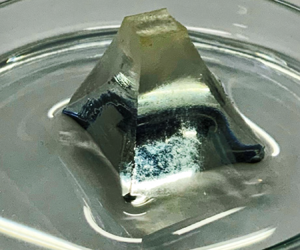
The utility of this new theory is most apparent in two- and three-dimensional problems, in which deviatoric strains can be generated by differential swelling. This is illustrated in figure 2, which shows an experiment in which a rectangular prism of hydrogel, fully swollen by immersion in water, is subsequently left to evaporate into the surrounding air while its base is maintained in contact with a reservoir of water. Details of the materials used in the experiment can be found in the supplementary material available at https://doi.org/10.1017/jfm.2023.201. The prism dries partially by evaporation, but reaches a steady state with transpiration of water from the dish, through the gel, and into the surrounding air. The key observation is that curvature is induced on the top and bottom surfaces of the gel and along the sides.

Figure 2. (a) A fully swollen rectangular prism of hydrogel (JRM Chemicals, Cleveland, Ohio, USA) removed from water, approximately  $3\,\mathrm {cm}$ high and $1\,\mathrm {cm}$ across. (b) The same prism more than $48$ h after its base was immersed in water while being allowed to evaporate from its other surfaces. By this time, the gel has reached a steady state with transpiration through it. (c) The prism removed from water, showing the curvatures of its base, top and sides, and that its aspect ratio has reduced from approximately $3\,:\,1$ to approximately $1\,:\,1$.
For simplicity, we consider the problem of a circular cylinder that dries by evaporation into the air, with initially uniform polymer fraction  $\phi _0$, radius $a_0$ and height $H_0$, where $\varepsilon = a_0 / H_0 \ll 1$. The base of the cylinder is held in water, and it is assumed throughout that this reservoir remains in contact with the base at all times and that the water within the reservoir is unlimited in supply, with uniform bulk water pressure $P=0$. The cylinder will shrink radially and vertically as water evaporates from the sides and top, and we seek to describe both the shape of the gel and the polymer fraction field, which quantifies the spatial variations in drying. At time $t$, the polymer fraction is given by $\phi (r, z, t)$, the height of the cylinder (measured along its axis at $r=0$) is $H(t)$, and – assuming that the gel remains axisymmetric throughout its drying – the radius is $a(z, t)$. We describe the curved bottom and top interfaces by $z=s_1(r, t)$ and $z=H(t)+s_2(r, t)$, respectively, as illustrated in figure 3. We seek the leading-order solutions in the small parameter $\varepsilon$ for each dependent variable.

Figure 3. (a) The initial state of a drying cylinder with uniform polymer fraction  $\phi _0$ and constant imposed evaporation fluxes $u_t$ and $u_s$ from the top and side surfaces, respectively. (b) The state of the cylinder at time $t$ after it has begun to dry, with curved lower and upper surfaces described by the functions $s_1(r, t)$ and $s_2(r, t)$, respectively, and a non-uniform value of $\phi$ along the axis. Note that the drying is greatest at the top where there is also more radial shrinkage, and that the base of the cylinder remains in full contact with the water for all time.
In order to describe the evaporative flux, we prescribe the Darcy flux on the surface of the cylinder. Drying from the sides is described by taking  $\boldsymbol {u}\boldsymbol {\cdot }\hat {\boldsymbol {n}} = u_s$ on $r=a(z, t)$, whilst drying from the top surface is described by $\boldsymbol {u}\boldsymbol {\cdot }\hat {\boldsymbol {n}} = u_t$ on $z=H(t)+s_2(r, t)$, where $\hat {\boldsymbol {n}}$ in each case is the unit normal to the surface pointing away from the gel.
For simplicity, we assume here that the shear modulus  $\mu _s$ of the gel and its permeability $k$ are both independent of polymer fraction $\phi$, and that the osmotic modulus $\varPi$ is a linear function of polymer fraction $\varPi (\phi ) = K_0 (\phi -\phi _0)/\phi _0$.
5.1. The polymer fraction field
In order to determine the polymer fraction field, we must solve the polymer fraction evolution equation (4.4) on the domain of the gel as it dries. We will then use this polymer fraction field to determine the shape of the domain, employing the displacement equation (4.3) to describe the deformation of individual gel elements. First, recall that all of the elements of  $\boldsymbol {\nabla } \phi$ must scale smaller than or equal to $\varepsilon /a_0$ under the assumption of small deviatoric strain (2.6), which implies that radial variations in polymer fraction are small relative to axial variations: order-unity axial variation is allowed since ${\partial \phi }/{\partial z} \sim \Delta \phi / H_0 \sim \varepsilon \,\Delta \phi / a_0$. This motivates separating the polymer fraction field into two parts,
 \begin{equation} \phi(r, z, t) = \phi_C(z, t) + \phi_1(r;z, t), \end{equation}
with  $\phi _1 = O(\varepsilon \phi _C)$, and, without loss of generality, $\phi _1(0;z, t) = 0$. Thus $\phi _C(z, t)$ represents the evolving polymer fraction along the axis $r=0$, while $\phi _1(r;z, t)$ encapsulates the relatively small radial variation of polymer fraction, with $z$ and $t$ as slowly varying parameters. Furthermore, because the total flux vector $\boldsymbol {q} = q_r \hat {\boldsymbol {r}} + q_z \hat {\boldsymbol {z}}$ is solenoidal, $q_r = O(\varepsilon q_z)$ since vertical length scales are a factor $1/\varepsilon$ greater than radial ones.
Thence, at leading order in  $\varepsilon$, the polymer fraction evolution equation (4.4) becomes
 $$\begin{gather} \frac{\partial \phi_C}{\partial t} + q_z\,\frac{\partial \phi_C}{\partial z} = \frac{\partial }{\partial z}\left[D(\phi_C)\,\frac{\partial \phi_C}{\partial z}\right] + \frac{1}{r}\,\frac{\partial }{\partial r}\left[r\,D(\phi_C)\,\frac{\partial \phi_1}{\partial r}\right], \end{gather}$$
 $$\begin{gather}\text{with}\quad D(\phi_C) = \hat{D}\left[\frac{\phi_C}{\phi_0} + \frac{4\mathcal{M}}{3}\left(\frac{\phi_C}{\phi_0}\right)^{1/3}\right], \end{gather}$$
where the basic diffusivity is  $\hat {D} = k K_0 / \mu _l$, and $\mathcal {M} = \mu _s/K_0$. This shows, firstly, that the relevant time scale for the cylinder drying is the axial diffusive time scale $t^* = H_0^2 / \hat {D} = a_0^2 / \hat {D} \varepsilon ^2$, which is long compared to the radial diffusive time scale $a_0^2/ \hat {D}$. Our formulation is valid for times $t \gg a_0^2/\hat {D}$. Secondly, the form of the equation allows us to separate variables for $r$, with the separation ‘constant’
 \begin{equation} S(z, t) = \frac{1}{D(\phi_C)}\left(\frac{\partial \phi_C}{\partial t} + q_z\,\frac{\partial \phi_C}{\partial z} - \frac{\partial }{\partial z}\left[D(\phi_C)\,\frac{\partial \phi_C}{\partial z}\right]\right) = \frac{1}{r}\,\frac{\partial }{\partial r}\left(r\,\frac{\partial \phi_1}{\partial r}\right). \end{equation}
The vertical material flux  $q_z$ is assumed to be a function of $z$ and $t$ only, as a result of slenderness, which is justified post hoc below in (5.33). Then, $\phi _1$ reaches a quasi-steady state
 \begin{equation} \phi_1 = \tfrac{1}{4}S(z, t)\,r^2 \end{equation}
on the (fast) radial diffusive time scale, once we impose regularity at  $r=0$. These radial variations drive the flow of water through the gel in the radial direction, therefore we can use the imposed evaporation flux on the surface of the gel at $r=a(z, t)$ to deduce the form of the function $S(z, t)$.
The leading-order Darcy velocity can be deduced in terms of polymer fraction gradients using a combination of Cauchy's momentum equation and Darcy's law, with radial component
 \begin{equation} u = \frac{D(\phi_C)}{\phi_C}\,\frac{\partial \phi_1}{\partial r} = \frac{D(\phi_C)\,S(z, t)}{2\phi_C}\,r, \end{equation}
and vertical component
 \begin{equation} v = \frac{D(\phi_C)}{\phi_C}\frac{\partial \phi_C}{\partial z}. \end{equation}
The normal to the sides of the cylinder is given by
 \begin{equation} \hat{\boldsymbol{n}} = \frac{\boldsymbol{\nabla}(r-a(z, t))}{\left|\boldsymbol{\nabla}(r-a(z, t))\right|} = \hat{\boldsymbol{r}} - \frac{\partial a}{\partial z}\,\hat{\boldsymbol{z}} + O(\varepsilon^2), \end{equation}
therefore the evaporation flux is
 \begin{equation} u_s \equiv \boldsymbol{u}\boldsymbol{\cdot}\hat{\boldsymbol{n}} = u-v\,\frac{\partial a}{\partial z} \end{equation}
to leading order, which gives
 \begin{equation} S = \frac{2\phi_C u_s}{D(\phi_C)\,a(z, t)} + \frac{2}{a(z, t)}\,\frac{\partial \phi_C}{\partial z}\,\frac{\partial a}{\partial z}. \end{equation}
This combines with (5.5) to show finally that
 \begin{equation} \phi_1(r; z, t) = \frac{\phi_C}{2a}\left\{\frac{\phi_C u_s}{\hat{D}} \left[\frac{\phi_C}{\phi_0} + \frac{4\mathcal{M}}{3}\left(\frac{\phi_C}{\phi_0}\right)^{1/3}\right]^{-1} + \frac{1}{\phi_C}\,\frac{\partial \phi_C}{\partial z}\,\frac{\partial a}{\partial z} \right\} r^2. \end{equation}
Now, since  $u_s \sim a_0 / t^*$, this result illustrates that in fact, $\phi _1 = O(\varepsilon ^2 \phi _C)$, a stronger result than our starting assumption of an order- $\varepsilon$ difference in scales.
5.2. The displacement field
In order to determine the shape of the cylinder as it dries, we first find the full axisymmetric displacement field  $\boldsymbol {\xi } = \xi \hat {\boldsymbol {r}} + \eta \hat {\boldsymbol {z}}$. We start with the $z$ component of the displacement equation (4.3):
 \begin{equation} \nabla^4 \eta =-3\,\frac{\partial }{\partial z}\nabla^2\left(\frac{\phi}{\phi_0}\right)^{1/3}. \end{equation}
Given (5.1) and (5.11), we find that the right-hand side is  $O(1/H_0^3)$, whilst the left-hand side, dominated by radial derivatives, is $O(\varepsilon /a_0^3)$. Therefore, the ratio of the right-hand side to the left-hand side is $O(\varepsilon ^2)$, and
 \begin{equation} \frac{1}{r}\,\frac{\partial }{\partial r}\left[r\,\frac{\partial }{\partial r}\left(\frac{1}{r}\,\frac{\partial }{\partial r}\left[r\,\frac{\partial \eta}{\partial r}\right]\right)\right] = 0 \end{equation}
to leading order. Integrating this equation and imposing regularity at  $r=0$ gives
 \begin{equation} \eta = A(z, t)\,r^2 + B(z, t), \end{equation}
where  $A$ and $B$ are arbitrary functions of vertical position $z$ and time $t$. Equation (4.2) for $\boldsymbol {\nabla } \boldsymbol {\cdot } \boldsymbol {\xi }$ then allows us to deduce that
 \begin{equation} \xi = \left\{ \frac{3}{2}\left[1-\left(\frac{\phi_C}{\phi_0}\right)^{1/3}\right] - \frac{1}{2}\,\frac{\partial B}{\partial z}\right\} r - \frac{1}{4}\,\frac{\partial A}{\partial z}\,r^3 \end{equation}
to leading order. Equations (5.14) and (5.15) allow us to write out the components of the deviatoric strain tensor at the same order:
 $$\begin{gather} \epsilon_{rr} = (1/2)\left[1-(\phi_C/\phi_0)^{1/3} - {\partial B}/{\partial z}\right] - (3/4) ({\partial A}/{\partial z})r^2, \end{gather}$$
 $$\begin{gather}\epsilon_{\theta \theta} = (1/2)\left[1-(\phi_C/\phi_0)^{1/3} - {\partial B}/{\partial z}\right] - (1/4)({\partial A}/{\partial z})r^2, \end{gather}$$
 $$\begin{gather}\epsilon_{zz} = {\partial B}/{\partial z} - 1 + (\phi_C/\phi_0)^{1/3} +({\partial A}/{\partial z}) r^2, \end{gather}$$
 $$\begin{gather}\epsilon_{rz} = \epsilon_{zr} = \left[A(z) - (3/4)(\partial/{\partial z})\left(\phi_C/\phi_0\right)^{1/3} - (1/4)({\partial^2 B}/{\partial z^2})\right]r \nonumber\\ - (1/8)({\partial^2 A}/{\partial z^2})r^3. \end{gather}$$
All other components of the tensor are zero to leading order in  $\varepsilon$. The requirement that $|\epsilon _{ij}| \lesssim \varepsilon$ allows us to deduce first that ${\partial A}/{\partial z}$ is order $\varepsilon / a_0^2$ or smaller, and also that
 \begin{equation} B(z, t) = \int^z_0{1-\left(\phi_C/\phi_0\right)^{1/3}\,\mathrm{d}z'} + C(z, t), \end{equation}
where  ${\partial C}/{\partial z}$ is $O(\varepsilon )$. Furthermore, the boundary condition $\eta (0, 0, t) = 0$, illustrated in figure 4, implies that $C(0, t)=0$.

Figure 4. A schematic diagram showing the boundary conditions imposed on the base and sides of the gel cylinder.
In order to determine the form of the two remaining unknown functions,  $A(z, t)$ and $C(z, t)$, it is necessary to appeal to boundary conditions on the stress tensor along the curved surface $r=a(z, t)$ of the cylinder.
5.2.1. Continuity of tangential stress
Requiring continuity of tangential stress  $\boldsymbol {n}\times {\boldsymbol {\sigma }}\boldsymbol {\cdot }\boldsymbol {n}$ implies that $\sigma _{rz} = 2\mu _s \epsilon _{rz} = 0$ on $r=a$ at leading order, therefore, using (5.16) for the deviatoric strain,
 \begin{equation} A = \frac{1}{2}\,\frac{\partial }{\partial z}\left(\frac{\phi_C}{\phi_0}\right)^{1/3} + O(\varepsilon^2/a_0). \end{equation}
This leaves  $C(z, t)$ as the only undetermined quantity. It also shows that the leading-order radial displacement is linear in $r$:
$r$:
 \begin{equation} \xi = \left[1-\left(\frac{\phi_C}{\phi_0}\right)^{1/3} - \frac{1}{2}\,\frac{\partial C}{\partial z}\right]r. \end{equation}
5.2.2. Continuity of normal stress
Continuity of normal stress  $\boldsymbol {n}\boldsymbol {\cdot }{\boldsymbol {\sigma }}\boldsymbol {\cdot }\boldsymbol {n}$ implies at leading order that $\sigma _{rr} = -P + 2\mu _s \epsilon _{rr} = 0$ on $r=a$. We use Cauchy's momentum equation $\boldsymbol {\nabla } \boldsymbol {\cdot } {\boldsymbol {\sigma }} = \boldsymbol {0}$ to find the bulk pressure field $P(r, z, t)$, the radial component of which equation gives
 \begin{equation} \frac{\partial P}{\partial r} = 2\mu_s\left[\frac{\partial \epsilon_{rr}}{\partial r} + \frac{\partial \epsilon_{rz}}{\partial z} + \frac{\epsilon_{rr} - \epsilon_{\theta \theta}}{r}\right] = O(\mu_s \varepsilon^2 / a_0), \end{equation}
owing to the fact that the shear term  ${\partial \epsilon _{rz}}/{\partial z}$ is of order $\varepsilon ^2/H_0$ in this case, as deduced above. Therefore, the bulk pressure is only a function of $z$ at leading order in the small parameter $\varepsilon$, as might be expected from the slenderness assumption. The vertical component of Cauchy's momentum equation implies that
 \begin{equation} \frac{\partial P}{\partial z} = 2\mu_s\left[\frac{\partial \epsilon_{zz}}{\partial z} + \frac{1}{r}\,\frac{\partial }{\partial r}(r\epsilon_{rz})\right]. \end{equation}
Differentiating this equation with respect to  $r$ and working up to terms of order $\varepsilon ^3$ gives
 \begin{equation} \frac{\partial }{\partial r}\left[\frac{1}{r}\,\frac{\partial }{\partial r}\left(r\epsilon_{rz}\right)\right] = O(\varepsilon^3/a_0^2), \quad \text{thus}\quad \epsilon_{rz} = F(z, t)\,r + O(\varepsilon^3), \end{equation}
where  $F(z, t)=O(\varepsilon ^2/a_0)$, and terms proportional to $1/r$ are neglected by requiring regularity along the $z$-axis. We reapply the condition of no tangential stress from above at $r=a$ to find $F \equiv 0$ and therefore $\epsilon _{rz}=0$ up to and including terms of order $\varepsilon ^3$. Hence (5.21) shows that
 \begin{equation} \frac{\partial P}{\partial z} = 2\mu_s\,\frac{\partial \epsilon_{zz}}{\partial z} + O(\mu_s \varepsilon^3 / a_0) = 2\mu_s\,\frac{\partial^2 C}{\partial z^2} + O(\mu_s \varepsilon^3 / a_0). \end{equation}
This gives  $P(z, t) = P_0(t) + 2\mu _s\,{\partial C}/{\partial z}$ for some spatially uniform $P_0$. The condition of no normal stress at the bottom interface between gel and water, for example applied at $r=z=0$, gives $\sigma _{zz} = 0$ here, and therefore $P_0 \equiv 0$. Hence, since $P = 2\mu _s\epsilon _{rr}$ on $r=a$,
 \begin{equation} 3\mu_s\,{\partial C}/{\partial z} = O(\mu_s\varepsilon^2), \quad \text{so}\quad C(z, t) = O(\varepsilon a_0). \end{equation}
5.2.3. The shape of the gel
Since  $C$ is order $\varepsilon a_0$, the radial displacement field is given at leading order in $\varepsilon$ by
 \begin{equation} \xi(r, z, t) = \left[1-\left(\frac{\phi_C}{\phi_0}\right)^{1/3}\right]r + O(\varepsilon^2 a_0), \end{equation}
which allows us to deduce the radius  $a(z, t)$, since $\xi$ is equal to $a-a_0$ on $r=a$. Therefore,
 \begin{equation} a(z, t) = \left(\phi_C/\phi_0\right)^{-1/3}a_0, \end{equation}
illustrating how the radial shrinkage is isotropic to leading order. Though we have not fully determined  $C$ here, the vertical displacement along the axis is given up to and including terms of order $a_0$ by
 \begin{equation} \eta(0, z, t) = \int^z_0{1-\left(\phi_C/\phi_0\right)^{1/3}\,\mathrm{d}z'}. \end{equation}
This allows us to determine  $H(t)$ through setting $z=H(t)$ and noting that $\eta (0, z, t) = H(t)-H_0$ on the top surface,
 \begin{equation} H_0 = \int^{H(t)}_0{\left(\phi_C/\phi_0\right)^{1/3}\,\mathrm{d}z'}, \end{equation}
with any contributions from the small term  $C(z, t)$ being zero at leading order. At leading order, the curvatures on the top and bottom interfaces (given by $s_1(r, t)$ and $s_2(r, t)$) are described by the order- $\varepsilon a_0$ radial variation in $\eta$, with
 \begin{equation} s_1(r, t) = \frac{r^2}{2}\left.\frac{\partial }{\partial z}\left(\frac{\phi_C}{\phi_0}\right)^{1/3}\right|_{z=0} \quad \text{and}\quad s_2(r, t) = \frac{r^2}{2}\left.\frac{\partial }{\partial z}\left(\frac{\phi_C}{\phi_0}\right)^{1/3}\right|_{z=H(t)}. \end{equation}
All of these quantities describing the shape of the gel as it dries are dependent on finding the axial polymer fraction  $\phi _C(z, t)$, for which we must return to the polymer fraction evolution equation (5.3).
5.2.4. Constraints on the aspect ratio
The components of the deviatoric strain tensor of (5.16) can all be seen to be  $O(\varepsilon ^2)$ or smaller in this case, where $\varepsilon$ is the aspect ratio $a_0/H_0$. It is discussed above how the key requirement for our linear-elastic–nonlinear-swelling model to apply to a situation is that all of the components of ${\boldsymbol {\epsilon }}$ are much smaller than $1$, i.e. that $\varepsilon ^2 \ll 1$. Therefore, our results here allow us to relax our initial slenderness assumption $\varepsilon \ll 1$, instead requiring only that
 \begin{equation} \left(a_0/H_0\right)^2 \ll 1. \end{equation}
Recall further from Part 1 that linear elasticity is valid only for small strains, where ‘small’ is defined by authors including Landau & Lifshitz (Reference Landau and Lifshitz1986) to be approximately  $10\,\%$. Therefore, instead of requiring an aspect ratio $H_0 \gtrsim 10 a_0$ for validity, this model should apply even in cases where $H_0 \gtrsim 3 a_0$, allowing us to model a wider range of drying cylinders.
5.3. Polymer fraction evolution
The expression for  $S$ in (5.10) can be combined with (5.4) to give the polymer fraction evolution equation
 \begin{equation} \frac{\partial \phi_C}{\partial t} + q_z\,\frac{\partial \phi_C}{\partial z} = \frac{\partial }{\partial z}\left[D(\phi_C)\,\frac{\partial \phi_C}{\partial z}\right] + \frac{2}{a}\left(\phi_C\,u_s + D(\phi_C)\,\frac{\partial \phi_C}{\partial z}\,\frac{\partial a}{\partial z}\right), \end{equation}
which rearranges to
 \begin{equation} \frac{\partial \phi_C}{\partial t} + q_z\,\frac{\partial \phi_C}{\partial z} = \frac{1}{a^2}\,\frac{\partial }{\partial z}\left[D(\phi_C)\,a^2\, \frac{\partial \phi_C}{\partial z}\right] + \frac{2 \phi_C u_s}{a}. \end{equation}
Equation (5.26) gives an expression for  $a$ that can be substituted in here. The vertical flux $q_z(z, t)$ remains to be found in order to result in an equation for $\phi _C$ that can be solved subject to boundary conditions, and used in turn to determine the radial variation $\phi _1$ using (5.11). To find the latter, we appeal to the definition of the total flux vector as the sum of the Darcy flux and the polymer velocity, as expressed in (4.9). Then, at leading order in $\varepsilon$,
 \begin{equation} q_z(z, t) = \frac{D(\phi_C)}{\phi_C}\,\frac{\partial \phi_C}{\partial z} - \left(\frac{\phi_C}{\phi_0}\right)^{1/3}\int^z_0{\frac{\partial }{\partial t}\left(\frac{\phi_C}{\phi_0}\right)^{1/3}\mathrm{d}z'}, \end{equation}
using the expression for  $\eta$ in (5.27). Notice that ${\partial q_z}/{\partial r} = 0$ at leading order, as postulated at the beginning. On the top surface at $z=H(t)$, $\hat {\boldsymbol {n}}\boldsymbol {\cdot }\boldsymbol {u} = u_t$, which reduces at leading order to requiring $v = u_t$ here. Hence a Neumann boundary condition is provided:
 \begin{equation} \frac{D(\phi_C)}{\phi_C}\,\frac{\partial \phi_C}{\partial z} = u_t \quad \text{on $z=H(t)$.} \end{equation}
It was also seen above that  $P = O(\mu _s \varepsilon ^2)$ throughout the gel. On the base, which is in contact with the bulk water, $p=0$ in addition, therefore the osmotic pressure is $\varPi = O(\mu _s \varepsilon ^2)$. This supplies the Dirichlet boundary condition $\phi _C = \phi _0$ on $z=0$.
5.4. Non-dimensional system
Alongside rewriting  $\phi _C/\phi _0 = \varPhi$, we introduce the other non-dimensional variables
 \begin{align} R = \frac{r}{a_0},\quad Z = \frac{z}{H_0},\quad \mathcal{H} = \frac{H}{H_0},\quad A = \frac{a}{a_0},\quad T = \frac{\hat{D} t}{H_0^2},\quad U_t = \frac{H_0 u_t}{\hat{D}},\quad U_s = \frac{H_0^2 u_s}{a_0\hat{D}}, \end{align}
which allows us to rewrite (5.32) as
 \begin{align} \frac{\partial \varPhi}{\partial T} + \left[\frac{2\,f(\varPhi)}{3}\,\frac{\partial \varPhi}{\partial Z} - \varPhi^{1/3}\int^Z_0{\frac{\partial \varPhi^{1/3}}{\partial T}\,\mathrm{d}Z'}\right]\frac{\partial \varPhi}{\partial Z} = \varPhi\,\frac{\partial }{\partial Z}\left[f(\varPhi)\,\frac{\partial \varPhi}{\partial Z}\right] + 2\varPhi^{4/3}U_s, \end{align}
where  $f(\varPhi ) = 1 + (4\mathcal {M}/3)\varPhi ^{-2/3}$. The boundary conditions are $\varPhi = 1$ at $Z = 0$, and
 \begin{equation} f(\varPhi)\,\frac{\partial \varPhi}{\partial Z} = U_t \quad \text{at }Z=\mathcal{H}(T). \end{equation}
The shape of the gel – and therefore the domain on which to solve the equation – is given by
 \begin{equation} A = \varPhi^{-1/3} \quad \text{and}\quad 1 = \int^{\mathcal{H}(T)}_0{\varPhi^{1/3}\,\mathrm{d}Z'}, \end{equation}
alongside
 \begin{equation} S_1 = \frac{\varepsilon^2 R^2}{2}\left.\frac{\partial \varPhi^{1/3}}{\partial Z}\right|_{Z=0} \quad \text{and}\quad S_2 = \frac{\varepsilon^2 R^2}{2}\left.\frac{\partial \varPhi^{1/3}}{\partial Z}\right|_{Z=\mathcal{H}(T)}, \end{equation}
where  $S_i = s_i/H_0$, scaling vertical displacements with the vertical length scale. The (small) radial variation in polymer fraction is given by
 \begin{equation} \varPhi_1 = \frac{\phi_1}{\phi_0} = \varepsilon^2\left[\frac{\varPhi^{1/3}U_s}{2\,f(\varPhi)} - \frac{1}{6\varPhi}\left(\frac{\partial \varPhi}{\partial Z}\right)^2\right] R^2. \end{equation}
 The numerical method that we used to solve this equation with its boundary conditions is outlined in the supplementary material. We will consider two special cases – firstly, where  $U_s = 0$, and secondly, where $U_t = 0$ – in order to understand the qualitative phenomena seen in experiments and how they relate to different aspects of the model.
Notice that the non-dimensionalisation here provides constraints on the size of the evaporative fluxes for the assumptions of our model to hold. By the scaling of (2.6), gradients in polymer fraction, radial and axial, would be too large for there to be small deviatoric strain throughout unless  $U_s\lesssim 1$ or $U_t \lesssim 1$, respectively. Using the non-dimensional scalings above, this implies that
 \begin{equation} u_s \lesssim a_0 D/H_0^2 \quad \text{and}\quad u_t \lesssim D/H_0. \end{equation}
Therefore, our model can support evaporation fluxes from the top surface that are  $O(1/\varepsilon )$ larger than their radial counterparts owing to slenderness. In either case, these two conditions are equivalent to requiring the radial and axial Péclet numbers to be at most order unity.
Recall that  $D$ has contributions from the pure diffusivity of the gel as a colloidal mixture ( $\hat {D}$), but is adjusted by shear modulus, with a greater value of $\mathcal {M}$ leading to a larger diffusivity. In the limit as $\mathcal {M}\to 0$, $D \to \hat {D}$ and it is the ‘pure diffusivity’ that provides the upper bounds on $u_s$ and $u_t$. As $\mathcal {M} \to \infty$, $D \to 4\mathcal {M}\hat {D} \varPhi ^{1/3}/3$ and the gel can support greater evaporative fluxes whilst still satisfying the requirements of small deviatoric strains. Therefore, increasing the shear modulus relative to the osmotic modulus, or drying the gel (so as to increase $\varPhi$ throughout), allows for ever-larger evaporative fluxes.
6. Modelling evaporation from the top and sides of a cylinder
We contrast the behaviour of cylinders where the drying occurs only from the top surface, with zero evaporation from the sides (non-zero  $U_t$ with $U_s=0$) with drying that occurs only from the sides and not from the top (non-zero $U_s$ with $U_t=0$). Though we are likely to observe a mixture of both of these behaviours in experiments, considering them separately allows us to understand the physics driving the different qualitative observations that can be made.
When drying from the top, (5.36) becomes an advection–diffusion equation (with no loss term  $2\varPhi ^{4/3}U_s$), and the radial variation in polymer fraction is
 \begin{equation} \varPhi_1 =-\frac{\varepsilon^2}{6\varPhi}\left(\frac{\partial \varPhi}{\partial Z}\right)^2 R^2. \end{equation}
This suggests that the polymer fraction decreases slightly towards the edges of the cylinder, which drives a small flow of interstitial fluid radially inwards, in order to impose the condition of no normal flux when the sides of the hydrogel slope outwards towards its base. The drying is initially localised around the top surface of the cylinder, until the gradient in polymer fraction formed along the axis of the cylinder draws water up from lower down, as illustrated in figure 5(a).

Figure 5. For a hydrogel with  $\mathcal {M}=1$ and initial dimensions $H_0 = 3a_0$, contour plots of the polymer fraction $\varPhi = \phi /\phi _0$ at four subsequent times through the drying process. (a) A gel with $U_t = 2.5$ and $U_s = 0$, showing the fact that shrinkage is initially localised at the top surface, and the formation of curved top and bottom interfaces. (b) A gel with $U_t = 0$ and $U_s = 2.5$, illustrating the flat top surface and the important radial gradients in $\phi$ that drive flow towards the sides of the cylinder.
If, on the other hand, drying occurs only from the side surface of the hydrogel, then there are two distinct phases of the subsequent evolution. Axial derivatives in polymer fraction are initially small, so (5.36) is dominated by the balance
 \begin{equation} \frac{\partial \varPhi}{\partial T} \approx 2\varPhi^{4/3}U_s. \end{equation}
This admits early-time solutions of the form  $\varPhi \approx (1-2U_s T / 3)^{-3}$, which result in radii $A \approx 1- 2U_s T / 3$, independent of $Z$. Eventually, diffusive and advective effects dominate as gradients along the $Z$ direction become appreciable. Unlike when drying from the top, the radial variation in polymer fraction takes the full form of (5.11), and therefore, for sufficiently large $U_s$, polymer fraction increases radially outwards, which supports the radial evaporative flux. Figure 5 shows the curved contours of $\phi$ that form in this case.
The differences in early-time drying behaviour are also apparent through considering the radius of the cylinders. Since initially only the top of the cylinder contracts when evaporating from the top surface alone, the radial contraction is restricted to this upper surface before continuing down the cylinder, as shown in figure 6(a). On the other hand, figure 6(b) shows how the radial contraction is initially approximately uniform, before differential drying along the axis of the cylinder (the base remains more swollen due to contact with the reservoir) becomes more apparent at later times.

Figure 6. Plots of the variation in the radius along the axis of a hydrogel as it evaporates into the air from (a) its top surface only, or (b) its sides only. In both cases,  $\mathcal {M} = 1$, $H_0 = 3a_0$, and the non-dimensional evaporative flux is $2.5$.
The top and bottom surfaces, described by  $S_1$ and $S_2$, also show another key difference between the top-drying and side-drying cases. Combining the expression for $S_2$ in (5.39b) with the Neumann boundary condition (5.37) on $Z=\mathcal {H}(T)$ implies that
 \begin{equation} S_2(R, T) = \left.\frac{\varepsilon^2 U_t R^2}{2\,f(\varPhi)\,\varPhi^{2/3}}\right|_{Z=\mathcal{H}(T)}. \end{equation}
Hence there is no curved top surface when drying from the sides, since  $U_t = 0$, as shown in figure 5.
Figure 5 indicates the existence of a steady state that is approached as evaporative fluxes from the gel surface become matched exactly by the interstitial flows of water from the base of the cylinder. Once this state, illustrated in figure 7, is reached, there is no longer any swelling or drying, but instead there is steady transpiration from the reservoir through the hydrogel. Varying  $\mathcal {M}$ affects both the rate at which this state is approached and also the form of the steady state, with there being significantly less shrinkage as $\mathcal {M}$ is increased. It is seen in figure 7 that a larger value of $\mathcal {M}$ leads to a more rapid approach to steady state, since the effective diffusivity $D(\phi _C)$ increases. Therefore, for a fixed evaporative flux $U_{t, s}$, there is less drying of the cylinder before this state is reached, leading to less shrinkage for larger $\mathcal {M}$. In addition, the steady state is reached when Darcy fluxes $\boldsymbol {u} = [D(\phi _C)/\phi _C]\,\boldsymbol {\nabla } \phi$ match evaporative fluxes, therefore a larger value of $D$ requires smaller values of $\boldsymbol {\nabla } \phi$ to reach equilibrium, again showing less shrinkage for larger $\mathcal {M}$.

Figure 7. The steady states reached by gels with  $H_0 = 3a_0$ drying from (a) their top and (b) their sides alone. (a i,b i) Representative shapes of the steady state for different evaporative fluxes, with $\mathcal {M}=1$. (a ii,b ii) Fixing the non-dimensional evaporative flux $U_s$ or $U_t$ to $2.5$, the contraction in height for a range of material parameters $\mathcal {M}$.
The approach to steady state can be understood as an equalisation of interstitial fluxes; at early times, the interstitial fluid flux is localised to the surface from which evaporation occurs, leading to drying of that region. The induced gradients in polymer fraction arising from this drying in turn drive flow from regions that are swollen to a greater degree, and this process continues until the rate at which water is fed into the system from the reservoir at the base of the gel matches the rate at which it is lost from the evaporating surface. Figure 8 shows the Darcy flux field  $\boldsymbol {u}$ at two different times for both cases, showing how these fluxes equalise as time progresses.

Figure 8. Plots of the interstitial flow field (the Darcy velocity  $\boldsymbol {u}$) in red, showing the fluxes at both early and late times.
7. Conclusion
In order to describe the behaviour of a hydrogel fully, it is necessary to solve both for its composition, described by the polymer fraction field  $\phi (\boldsymbol {x}, t)$, and also for its shape, which we can deduce from the displacement field $\boldsymbol {\xi }(\boldsymbol {x}, t)$. This displacement field is also needed to find the polymer velocity (and therefore the phase-averaged flux $\boldsymbol {q}$) and the deviatoric strain ${\boldsymbol{\mathsf{\epsilon}}}$, which gives the stress field in the hydrogel. In Part 1, it was shown that for one-dimensional swelling problems, $\boldsymbol {\xi }$ and $\phi$ could be related straightforwardly by conservation of polymer, while $\boldsymbol {\nabla }\boldsymbol {\cdot }\boldsymbol {q}=0$ allowed us to deduce the total flux vector, providing a complete description of these simpler physical situations.
In this paper, we have shown how the displacement field can be deduced from the polymer fraction field, solving a forced biharmonic equation with a forcing arising from gradients in polymer fraction through the hydrogel. Parallels between this result of linear-elastic–nonlinear-swelling theory and linear elasticity can be drawn easily, with the displacement field given by our model reducing to the biharmonic displacement field of linear elasticity in the absence of gradients in  $\phi$, corresponding to our founding assumption that a hydrogel behaves on short time scales as a linear-elastic material.
Given  $\phi$ and $\boldsymbol {\xi }$, it is possible thus to deduce an expression for the phase-averaged flux $\boldsymbol {q}$, with contributions from both the flow of water through the polymer scaffold and the deformation of the polymer itself, and therefore the evolution of $\phi$ in time can be described using only our knowledge of $\phi$ at a given time, alongside prescribed boundary conditions. These conditions can apply to the displacement field itself (rigid walls, or no-slip conditions at the edges of a gel), the bulk stress ${\boldsymbol {\sigma }}$ (continuity of normal or tangential stress) or the pervadic pressure $p$ (continuity of pervadic pressure or flux conditions), all of which we can now deduce given the form of the polymer fraction field $\phi (\boldsymbol {x}, t)$. This model is applicable when the deviatoric strains are small, and does not rely on any assumptions on the direction of swelling or the symmetry of the situation, unlike the cases considered in Part 1, and in principle allows us to describe the evolution of any gel satisfying the founding assumption of small deviatoric strains using a system of coupled partial differential equations alongside the aforementioned boundary conditions.
We have illustrated the utility of this model by considering the example of hydrogels drying into air by evaporation with their bases submerged in water, leading to steady transpiration at late times. In these examples, the evolution equation for polymer fraction and the displacement equation describe the composition and shape of the hydrogel, respectively, as it dries, and we have shown specifically how the displacements of individual gel elements depend on  $\phi$ and its gradient. The results derived from this model give good qualitative agreement with experiments that we have carried out, and provide a physical explanation for phenomena seen in these experiments, such as the formation of curved gel–air interfaces and the approach to a steady state where evaporative fluxes match imbibition fluxes from the reservoir of water in which the cylinders are sat. An alternative physical interpretation of these results, in the simpler case where all of the evaporation occurs from the top of a cylinder, is provided in Appendix A, showing how assuming locally isotropic drying and using the equations of classical plate theory leads to the same result for the displacement field. However, as mentioned above, a strength of our model is its generality in not requiring such simplifying assumptions to be made.
Together with the founding assumptions of Part 1, we have illustrated here how our linear-elastic–nonlinear-swelling theory can describe hydrogels in a wide variety of situations, and requires only the assumption of small deviatoric strains to be applicable. We have shown that this condition can be met with large variations in polymer fraction provided that  $\mathcal {M}=\mu _s/K_0$ is large, as was seen in Part 1. In the specific evaporating system that we analysed, this condition was met provided that the Péclet numbers $u_t H_0 / D$ and $u_s H_0 / \varepsilon D$ are both order unity or smaller, noting that the diffusivity $D$ increases with $\mathcal {M}$.
Supplementary material
Supplementary material is available at https://doi.org/10.1017/jfm.2023.201.
Funding
J.J.W. is supported by the Natural Environment Research Council (project reference 2436164) through the Cambridge Climate, Life and Earth Sciences DTP (NE/S007164/1). M.A.E. gratefully acknowledges funding from the Centre for Natural Materials Innovation funded by the Leverhulme Trust.
Declaration of interests
The authors report no conflict of interest.
Appendix A. Lagrangian model for a cylinder evaporating from the top
As alluded to in § 2, the displacement equation bears a resemblance to the governing equations of classical (Kirchhoff–Love) plate theory (Landau & Lifshitz Reference Landau and Lifshitz1986). The drying cylinder, with polymer fraction that varies only in the vertical direction, can be viewed as a stack of thin discs, each of which has a uniform polymer fraction  $\phi _i$ and deforms as a plate under a load, as illustrated in figure 9. The loading here on an individual plate is set by considering the forces on the system arising from the stress tensor introduced in Part 1. Given that we can solve (5.36) with appropriate boundary conditions (as described above) to supply the leading-order polymer fraction field $\phi _C(z, t)$, it is shown that this ‘naïve’ Lagrangian approach provides a physical basis for the displacement formulation that we have derived, showing the equivalence between classical plate theory and our displacement formulation in this special case.

Figure 9. (a) The division of the fully swollen hydrogel into Lagrangian reference slices of thickness  $h_0$, all with uniform radius $a_0$. In time, these slices shrink isotropically to new thicknesses $h_i$ and new radii $a_i$, as illustrated in (b), but in order for radial strains to match between slices, this requires the individual thin elements to bend, as illustrated in (c).
The key assumption of our model, that deviatoric strains are small, is equivalent to stating that swelling and drying are locally isotropic at leading order: that is, in a given Lagrangian slice where the axial polymer fraction  $\phi _C$ is $\phi _i$, the Cauchy strain tensor is approximately equal to $[1-(\phi _i/\phi _0)^{1/3}]\boldsymbol{\mathsf{I}}$. In the fully swollen state, in which each Lagrangian layer is swollen with $\phi =\phi _0$, the slices have radii $a_i = a_0$ and thickness $h_i = h_0$. Now, assume that each layer contracts isotropically and seek the order- $\varepsilon$ correction to the displacement that results from matching adjacent layers. To begin, the leading-order isotropic shrinkage implies that
 \begin{equation} a_i = \left(\phi_i/\phi_0\right)^{-1/3}a_0 \quad \text{and}\quad h_i = \left(\phi_i/\phi_0\right)^{-1/3}h_0. \end{equation}
Now realise that differential drying leads to differential shrinkage, as shown in figure 9(b). The intermediate situation pictured here is unphysical since there are discontinuities in the radial strain. The only way to prevent such discontinuities is if the layers bend under loading to match their neighbours, introducing the concavity and convexity seen on the top and bottom surfaces, respectively, in figure 2. This curvature is shown in figure 9(c), illustrating how it accommodates the differential drying.
In order to describe the deflection of a thin, linear elastic, plate under loading, we appeal to Kirchhoff–Love plate theory. Assuming that the deflection leads to a radial displacement  $\gamma$ and a vertical displacement $\zeta$, the assumptions of classical plate theory can be applied to this displacement field $\gamma \hat {\boldsymbol {r}} + \zeta \hat {\boldsymbol {z}}$. These assumptions underpin a number of theories and have been well-described in the literature (see, for example, Timoshenko & Woinowsky-Krieger Reference Timoshenko and Woinowsky-Krieger1959; Landau & Lifshitz Reference Landau and Lifshitz1986). Start by introducing a coordinate system centred on the midpoint of the plate, with radial coordinate $r$ and vertical coordinate (aligned with the axis of the cylinder) $z_p$. Firstly, there are no midplane strains, which gives $\gamma =0$ along the centre of the layer $z_p = \zeta (r, 0)$. Secondly, the assumption that normals to the midplane of the plate remain normal to this plane under deformation imposes ${\partial \gamma }/{\partial r} + {\partial \zeta }/{\partial z_p} = 0$. Finally, the equation of equilibrium gives
 \begin{equation} \nabla^4 \zeta =-Q/\mathfrak{D}, \end{equation}
where  $Q$ is the load, and $\mathfrak {D}$ is the bending stiffness. The load in this case is equal to the force exerted normal to the plate, and is therefore given by ${\partial \sigma _{zz}}/{\partial z} = 0$. Therefore, in the absence of shear stresses at leading order, $Q=0$, representing an elastic plate under so-called pure bending. Thus the value of $\zeta (r)$ can be deduced to be a biharmonic function (a special case of the Michell solution; Michell Reference Michell1899). Imposing regularity conditions at $r=0$, this solution must take the form
 \begin{equation} \zeta(r) = W + V r^2, \end{equation}
for some constants  $W$ and $V$ to be determined from boundary conditions. This equation represents a deflection of the plate with curvature $2V$. Now, applying the condition that normal elements remain normal, $\gamma (r, z_p) = -2V z_p$, using $\gamma (r, 0) = 0$ to set the arbitrary constant.
Matching the radial strains at the interface between slice  $i$ and slice $i+1$, using the leading-order isotropic displacement field, gives
 \begin{equation} 1- \left(\phi_i/\phi_0\right)^{1/3} - V_i h_i = 1- \left(\phi_{i+1}/\phi_0\right)^{1/3} + V_{i+1} h_{i+1}. \end{equation}
We collect these terms and write  $h_i$ and $h_{i+1}$ in terms of $\phi _i$ and $\phi _{i+1}$:
 \begin{equation} 2h_0\left[\left(\frac{\phi_{i+1}}{\phi_0}\right)^{1/3} V_{i+1} + \left(\frac{\phi_i}{\phi_0}\right)^{1/3}V_{i}\right] = \left(\phi_{i+1}/\phi_0\right)^{1/3} - \left(\phi_i/\phi_0\right)^{1/3}. \end{equation}
Finally, taking the limit  $h_0 \to 0$ gives the value of $V$ and hence
 \begin{equation} \zeta = W + \frac{1}{2}\,\frac{\partial }{\partial z}\left(\frac{\phi}{\phi_0}\right)^{1/3} r^2. \end{equation}
Since the expression for  $\gamma$ above gives $\gamma \sim h_i V \ll 1$, we find
 $$\begin{gather} \xi = \left[1-\left(\frac{\phi}{\phi_0}\right)^{1/3}\right]r + O(\varepsilon^2 a_0), \end{gather}$$
 $$\begin{gather}\eta = \int^{z}_0{1-\left(\frac{\phi}{\phi_0}\right)^{1/3}\mathrm{d}u} + \frac{1}{2}\,\frac{\partial }{\partial z}\left(\frac{\phi}{\phi_0}\right)^{1/3}r^2 + C(z) + O(\varepsilon^2 a_0), \end{gather}$$
again with an undetermined  $C(z)$ of order $\varepsilon a_0$, given by $W$ at the position $z$. Notice here that the displacement field that we have derived satisfies (4.3) up to terms of order $\varepsilon ^2$. This can be interpreted as the superposition of a leading-order swelling displacement with an elastic displacement of order $\varepsilon a_0$. Though entirely equivalent to the displacement formulation derived above, this alternative approach supplies a physical justification for the curvature terms in the displacement field.


 Open access