


1. Introduction
Hydrogels are an important class of materials composed of a hydrophilic polymer scaffold surrounded by adsorbed water molecules. The interstitial water is nevertheless free to flow through the matrix formed by the polymer chains, which create a structure that can be treated as a porous medium (Doi Reference Doi2009; MacMinn, Dufresne & Wettlaufer Reference MacMinn, Dufresne and Wettlaufer2016; Punter, Wyss & Mulder Reference Punter, Wyss and Mulder2020). In recent years, there has been much interest in super-absorbent polymers (SAPs), which can swell to several hundred times their dry volume when placed in water (Bertrand et al. Reference Bertrand, Peixinho, Mukhopadhyay and MacMinn2016), owing to the extremely hydrophilic nature of the polymer constituting the scaffold.
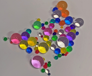
Perhaps the most recognisable consumer application of hydrogels over the last decade has been the children's toy OrbeezTM, illustrated in figure 1, which has achieved widespread international popularity (Forrester Reference Forrester2019). Domestically, such gels have found increasing use as water-retention beads for potted plants (Chang et al. Reference Chang, Xu, Liu and Qiu2021; Souza et al. Reference Souza, Guimarães, Dominghetti, Scalco and Rezende2016) and the absorbent material used in nappies (Al-Jabari, Ghyadah & Alokely Reference Al-Jabari, Ghyadah and Alokely2019). Aside from this, hydrogels are an increasingly important class of materials with a range of applications in the life sciences: from biocompatible contact lenses (Wichterle & Lím Reference Wichterle and Lím1960; Moreddu, Vigolo & Yetisen Reference Moreddu, Vigolo and Yetisen2019) and cancer treatment (Li et al. Reference Li, Ding, Liu, Wang, Mo, Wang, Chen-Mayfield, Sondel, Hong and Hu2022) to wound dressings (Op ’t Veld et al. Reference Op ’t Veld, Walboomers, Jansen and Wagener2020); in agriculture (Guilherme et al. Reference Guilherme, Aouada, Fajardo, Martins, Paulino, Davi, Rubira and Muniz2015); as a fire-retardant coating in areas prone to wildfires (Toreki Reference Toreki2005); and to control flow in porous rock during enhanced oil recovery (Pu et al. Reference Pu, Zhou, Chen and Bai2017). Alongside these newer applications, the ability of hydrogels to take up water and swell to many hundreds of times their initial volume has led to a number of established uses in the field of personal care as well as in construction, as a concrete additive to reduce chemical shrinkage during curing and alter the rheology of sprayed concrete (Jensen & Hansen Reference Jensen and Hansen2002; Jensen Reference Jensen2013), and in other industrial fields (Zohuriaan-Mehr et al. Reference Zohuriaan-Mehr, Omidian, Doroudiani and Kabiri2010). It has also been suggested by some authors, including Zwieniecki, Melcher & Holbrook (Reference Zwieniecki, Melcher and Holbrook2001), that naturally occurring hydrogels have a role to play in the flow of water through the xylem conduits of vascular plants.

Figure 1. An illustration of different stages of swelling of a super-absorbent gel sold as the children's toy OrbeezTM, showing the state in equilibrium with typical indoor conditions on the left and the fully swollen state after immersion in water for some hours on the right.
In this paper, there are two key gel behaviours that we wish to capture: the large-swelling nature that characterises super-absorbent hydrogels, and the fact that the interstitial fluid is able to flow through the gel matrix, which behaves as a poroelastic medium. However, whereas many authors conceptualise the matrix and fluid separately, we take the view that the hydrogel (matrix plus fluid) is the material that we describe. In particular, we work in terms of the elasticity of the whole material, the gel, rather than the elasticity of the matrix as a property independent of the interstitial fluid. We also reserve the term elastic response to mean the instantaneous response of the gel to an applied load, i.e. on timescales much shorter than the scale for redistribution of water within the gel. Thus, we treat the gel as incompressible even though the matrix is compressible (Doi Reference Doi2009). In general, a hydrogel is an inhomogeneous material, with material properties that depend on the local polymer fraction, as we shall describe.
The dynamics of hydrogels is closely related to poromechanics (Coussy Reference Coussy2004), the existing modelling of which can be classed into two broad groups, which we refer to as fully linear and fully nonlinear. Fully linear models, such as those described by Biot (Reference Biot1941) and detailed by Doi (Reference Doi2009), build on the approach introduced by Terzaghi (Reference Terzaghi1925) in soil mechanics, considering the liquid phase and the solid phase separately and seeking a constitutive relation for the effective stress of the matrix, a polymer-fraction-weighted stress tensor with contributions from each of the two phases. These models apply a linear-elastic constitutive relation (Landau & Lifshitz Reference Landau and Lifshitz1986) for this effective stress tensor and describe the dynamics of the hydrogel swelling and drying using Darcy's law to govern the interstitial flow. Though this captures the characteristic of hydrogels as poroelastic media through which water can flow (Punter et al. Reference Punter, Wyss and Mulder2020), such descriptions do not adequately explain the large-swelling behaviour seen in super-absorbent hydrogels. Linear-elastic theories require linearisation with respect to small strains relative to some pre-ordained reference state. These strains should be smaller than around  $10\,\%$ (Landau & Lifshitz Reference Landau and Lifshitz1986) for the predictions to be considered accurate, corresponding, in three dimensions, to volumetric changes of less than about $30\,\%$.
It is for this reason that many authors, including Bertrand et al. (Reference Bertrand, Peixinho, Mukhopadhyay and MacMinn2016), Chester & Anand (Reference Chester and Anand2011), Hong et al. (Reference Hong, Zhao, Zhou and Suo2008) and Butler & Montenegro-Johnson (Reference Butler and Montenegro-Johnson2022) invoke fully nonlinear descriptions of gels. Many such approaches are based on the work of Flory & Rehner (Reference Flory and Rehner1943a,Reference Flory and Rehnerb), who derive a free-energy density function  $\mathcal {W}$ that is separated into contributions from mixing of water and polymer components $\mathcal {W}_{{mix}}$ and stretching of polymer chains $\mathcal {W}_{{stretch}}$. Expressions for these two functions are generally sought from a microscopic understanding of the molecules involved, with Flory–Huggins theory (Flory Reference Flory1953) giving $\mathcal {W}_{{mix}}$ (a summed contribution of entropy and enthalpy of mixing) and, traditionally, a Gaussian–Chain model used for $\mathcal {W}_{{stretch}}$ to describe the elasticity of individual long polymer molecules (Flory & Rehner Reference Flory and Rehner1943a). Other authors, including Drozdov et al. (Reference Drozdov, Papadimitriou, Liely and Sanporean2016) and Hennessy, Münch & Wagner (Reference Hennessy, Münch and Wagner2020), use more general Neo–Hookean constitutive relations for the strain-energy density. A review of such models is given by Boyce & Arruda (Reference Boyce and Arruda2000). Principal stresses can be found from such energy densities, and it is then possible to separate the contributions from pore pressure and an effective stress in a similar approach to Terzaghi (Reference Terzaghi1925), as shown by Bertrand et al. (Reference Bertrand, Peixinho, Mukhopadhyay and MacMinn2016), for example. Although it is noted that such descriptions reduce to standard poroelasticity when mixing contributions are negligible, the complicated nature of the function $\mathcal {W}$ and the reliance on a full understanding of small-scale electrostatic effects means that the physical intuition into gel behaviour that can be gained from using this approach is more difficult than with the fully linear case.
In an alternative approach to describing large strains in soft porous materials, MacMinn et al. (Reference MacMinn, Dufresne and Wettlaufer2016) develop a model employing large-deformation poroelasticity to describe the mechanical response of the matrix. Here, the approach found in the fully linear Biot model of poroelasticity is augmented with a nonlinear elastic constitutive relation. However, the use of large-deformation elastic models, in this case Hencky elasticity, introduces nonlinearities into the constitutive relation which render the elastic deformation difficult to solve for analytically. Furthermore, it becomes a matter of discussion as to which hyperelastic constitutive model should be employed to describe a hydrogel: the choice by MacMinn et al. (Reference MacMinn, Dufresne and Wettlaufer2016) of Hencky elasticity is purely used as a demonstration, with an array of other such models in existence (Marckmann & Verron Reference Marckmann and Verron2006).
Our approach is intermediate between the fully linear and fully nonlinear models. We start by noting that, in many practical situations, the very large deformations associated with swelling or shrinkage are dominated by locally isotropic strains that are not associated with macroscopic stresses. In each of the stages of swelling, shown in figure 1, for example, the beads, considered as bulk materials, are elastically unstressed; although there are stresses in the matrix due to stretching of polymer chains, these are exactly balanced by pressures in the fluid. At any stage of swelling, each bead can be subjected to deviatoric stresses (e.g. by pressing between thumb and forefinger) that can give rise to small deviatoric strains that can be described using linear elasticity with respect to the isotropically swollen state. Alternatively, deviatoric strains can be induced internally by differential swelling, but in many cases can remain small relative to this same (locally) isotropic swelling state. The linear-elastic-nonlinear-swelling (LENS) theoretical framework we develop in this paper is founded on the consideration of hydrogels as instantaneously incompressible poroelastic media that can undergo arbitrarily large, locally isotropic, strains by swelling in response to fluid flow, while behaving linearly elastically with respect to deviatoric strains and stresses. This approach gives rise to a system of governing equations for the elasticity that are significantly more tractable than fully nonlinear models, whilst retaining nonlinearities in equations governing the swelling. It allows us to make continuum-mechanical predictions of gel behaviour, including many situations with large deformations, given just three readily measurable material parameters with analogues in classical linear poroelasticity.
We start in § 2 by separating isotropic and deviatoric strains and relating the former to the polymer fraction field in the gel. A constitutive relation that allows for nonlinearity only in the swelling is then introduced in § 3 before we find an expression for the interstitial fluid velocity in § 4. Conservation of momentum, when combined with our constitutive relation and Darcy's law, allows us to link the elastic response to the interstitial fluid velocity and gives a set of equations describing the evolution of polymer fraction  $\phi$ in time. A simple rheometer experiment is detailed in § 5 that, in principle, allows for the determination of all three material parameters that describe a hydrogel: an osmotic modulus $K(\phi )$, an elastic shear modulus $\mu _s(\phi )$ and a permeability $k(\phi )$, each a function of the polymer volume fraction $\phi$. Finally, we apply this model to two basic gel swelling problems: first, a gel swelling between horizontal confines (§ 6), illustrating the importance of the deviatoric strains in setting equilibrium polymer fractions and the effective diffusivity of the medium; secondly, a swelling bead similar to that considered by Bertrand et al. (Reference Bertrand, Peixinho, Mukhopadhyay and MacMinn2016) and Punter et al. (Reference Punter, Wyss and Mulder2020) (§ 7), showing how, for particular choices of material parameters, large isotropic strains can be attained while deviatoric strains remain small at all times.
In Part 2 (Webber, Etzold & Worster Reference Webber, Etzold and Worster2023), we extend our approach to the more general case in which swelling is no longer confined to a single direction and differential swelling leads to large-scale changes of shape. In such cases, polymer fractions and displacements cannot be so straightforwardly related and new relations are needed to link the polymer transport equation derived here with more complicated deformations.
2. Displacements and strains
In all elastic theories, deformations are described relative to some reference state that must be defined carefully. It is not immediately apparent what the reference state for a hydrogel should be. Some authors including Kang & Huang (Reference Kang and Huang2010) and Bertrand et al. (Reference Bertrand, Peixinho, Mukhopadhyay and MacMinn2016), who focused on the elasticity of the polymer scaffold, use a fully dry polymer with no water content as their reference state, reasoning that the polymer chains are completely unstretched in this case. Others, such as Doi (Reference Doi2009) and Etzold, Linden & Worster (Reference Etzold, Linden and Worster2021), introduce the concept of a ‘fully swollen equilibrium’ state, a convention that we follow here. This is defined to be the final state reached by a gel immersed in water and subject to no external forces, with all of the hydrogel swollen uniformly and in thermodynamic equilibrium. An expression for the equilibrium polymer fraction can be found in principle from an understanding of the microscopic structure of the gel (see, e.g., Appendix A), depending on temperature and the number of cross-links per unit length in the polymer chains. However, here we take a macroscopic view and will later show how the relevant material properties can be determined experimentally.
We introduce coordinates  $\boldsymbol {X}$ to denote the positions of gel elements in this equilibrium state, and describe any kind of general deformation, be that an elastic deformation of the gel behaving as a rubber-like material or a swelling or drying of the gel as water is taken up or expelled, by a transformation into coordinates $\boldsymbol {x}(\boldsymbol {X},t)$, each with respect to a fixed (Eulerian) frame of reference. We define
 \begin{equation} \boldsymbol{\mathsf{F}} = \boldsymbol{\nabla}_{\boldsymbol{X}}{\boldsymbol{x}} \quad \text{i.e.} \ {\mathsf{F}}_{ij} = \frac{\partial x_i}{\partial X_j} \end{equation}
as the deformation gradient tensor, or Jacobian matrix, for this transformation. The Jacobian determinant  $J=\operatorname {det}\boldsymbol{\mathsf{F}}$ represents the scale factor by which the volume of a gel element increases under such a transformation.
We make the assumption that, macroscopically, the hydrogel is instantaneously incompressible, so the only way that the volume of a gel element containing a fixed quantity of polymer can change is by the flow of water either into or out of the element, hence changing the volume fraction occupied by polymer. If we denote the polymer volume fraction by  $\phi$, with $\phi _0$ the equilibrium polymer fraction, it is readily understood that
 \begin{equation} J = \frac{\phi_0}{\phi} \end{equation}
at each point in the gel. We now separate the deformation gradient tensor into isotropic and deviatoric parts by writing
 \begin{equation} \boldsymbol{\mathsf{F}} = \mathcal{F}\boldsymbol{\mathsf{I}} + \boldsymbol{\mathsf{f}}. \end{equation}
Here,  $\mathcal {F}$ represents the isotropic part of the tensor and $\boldsymbol{\mathsf{f}}$ is the deviatoric part, where, in $n$ spatial dimensions, $\mathcal {F} = \operatorname {tr}\boldsymbol{\mathsf{F}}/n$ and $\operatorname {tr}\boldsymbol{\mathsf{f}} = 0$, with $\boldsymbol{\mathsf{I}}$ the $n\times n$ identity matrix. This separates deformation due to swelling and drying (the isotropic part) from deformation due to shearing (the deviatoric part). Writing $\boldsymbol{\mathsf{F}}$ in this manner allows us to encode our assumption that strains due to swelling may be large while linear elasticity applies for deviatoric deformations provided that $\boldsymbol{\mathsf{f}}$ is small (i.e. $|\,{\mathsf{f}}_{ij}| \ll 1$ for all $i,\,j$). Such an assumption can be expected to hold in many cases of practical importance, the only exceptions being cases in which gradients in polymer fraction $\boldsymbol {\nabla } \phi$ are large, in a sense to be defined formally later, such as in the phase-separation behaviour discussed by Hennessy et al. (Reference Hennessy, Münch and Wagner2020), where the liquid and polymer phases separate into distinct regions, with $|\boldsymbol {\nabla }\phi |$ large at the boundary between these regions.
Using the Taylor series expansion for the determinant of a matrix close to the identity (Petersen & Pedersen Reference Petersen and Pedersen2012),
 \begin{equation} \operatorname{det}\left(\boldsymbol{\mathsf{I}} + \epsilon \boldsymbol{\mathsf{A}}\right) = 1 + \epsilon \operatorname{tr}\boldsymbol{\mathsf{A}} + O(\epsilon^2), \end{equation}
where  $\epsilon$ is a small scalar, we can compute the determinant of $\boldsymbol{\mathsf{F}}$ in terms of $\mathcal {F}$ to first order in the small deviatoric strain,
 \begin{align} J=\operatorname{det}\left(\mathcal{F}\boldsymbol{\mathsf{I}} + \boldsymbol{\mathsf{f}}\right) = \mathcal{F}^n\operatorname{det}\left(\boldsymbol{\mathsf{I}} + \mathcal{F}^{-1}\boldsymbol{\mathsf{f}}\right) &= \mathcal{F}^n\left[1+\mathcal{F}^{-1}\operatorname{tr}\boldsymbol{\mathsf{f}} + O(\boldsymbol{\mathsf{f}}^2)\right] \nonumber\\ &= \mathcal{F}^n + O(\boldsymbol{\mathsf{f}}^2). \end{align}
Therefore, to leading order,  $J = \mathcal {F}^n$ and the deformation gradient tensor of (2.3) can be rewritten
 \begin{equation} \boldsymbol{\mathsf{F}} = \left(\frac{\phi}{\phi_0}\right)^{-1/n}\boldsymbol{\mathsf{I}} + \boldsymbol{\mathsf{f}}. \end{equation}
2.1. The Cauchy strain tensor
Our model, as mentioned previously, is linear-elastic relative to a reference state of isotropic swelling, with all nonlinearities encapsulated by the swelling and drying state of the material. There are a number of strain measures used in finite-strain elasticity, incorporating nonlinear effects and generalising the Cauchy strain tensor of linear elasticity to capture the influence of potentially large displacements. Many theories simply use the deformation gradient tensor  $\boldsymbol{\mathsf{F}}$ or the Cauchy–Green deformation tensors $\boldsymbol{\mathsf{F}}\boldsymbol{\mathsf{F}}^{{T}}$ and $\boldsymbol{\mathsf{F}}^{{T}}\boldsymbol{\mathsf{F}}$. The choice of strain measure is largely arbitrary, and is usually made to simplify the constitutive relation for the stress. Our model requires a linear relationship between stresses arising from deviatoric strains and these deviatoric strains themselves, and we therefore use the Cauchy strain tensor of linear elasticity. We show in Appendix B that, even starting from a fully hyperelastic model, once the assumption of small deviatoric strain is applied, the stress can be written in terms of the deviatoric Cauchy strain in addition to a nonlinear isotropic part.
When defining our strain tensor it is also important to consider carefully whether the quantities under consideration are Lagrangian or Eulerian. In linear elasticity, this is less important because the small deformations are the same to leading order in both descriptions of the problem whilst here, with potentially large total strains, this is no longer the case. We start by defining the displacement  $\boldsymbol {\xi } = \boldsymbol {x} - \boldsymbol {X}$. The Cauchy strain tensor is then defined by
 \begin{equation} \boldsymbol{\mathsf{e}} = \tfrac{1}{2}\left[\boldsymbol{\nabla}_{\boldsymbol{x}}\boldsymbol{\xi}+\left(\boldsymbol{\nabla}_{\boldsymbol{x}}\boldsymbol{\xi}\right)^{\rm T}\right], \end{equation}
where  $\boldsymbol {\nabla }_{\boldsymbol {x}}$ denotes a gradient taken with respect to the deformed, Eulerian, coordinates. Even though, for large deformations, it may appear that a Lagrangian description of the gel would be more tractable when dealing with swelling problems, it is noted by MacMinn et al. (Reference MacMinn, Dufresne and Wettlaufer2016) that an Eulerian description often tends to be preferable for poroelastic problems, since the equations governing the fluid flow tend to be stated in an Eulerian framework. Coupling is easier if one consistently uses the same description. We can calculate the value of $\boldsymbol {\nabla }_{\boldsymbol {x}}\boldsymbol {\xi }$ in terms of $\boldsymbol{\mathsf{F}}$ using the chain rule because
 \begin{align} \boldsymbol{\nabla}_{\boldsymbol{x}}\boldsymbol{\xi} = \boldsymbol{\nabla}_{\boldsymbol{X}}\boldsymbol{\xi}\boldsymbol{\cdot} \boldsymbol{\nabla}_{\boldsymbol{x}}\boldsymbol{X} &= \left[\boldsymbol{\nabla}_{\boldsymbol{X}}\boldsymbol{x} - \boldsymbol{\mathsf{I}}\right]\boldsymbol{\cdot}\boldsymbol{\nabla}_{\boldsymbol{x}}\boldsymbol{X} \nonumber\\ &= \boldsymbol{\mathsf{F}}\boldsymbol{\mathsf{F}}^{-1} - \boldsymbol{\mathsf{F}}^{-1} \nonumber\\ &= \boldsymbol{\mathsf{I}} - \boldsymbol{\mathsf{F}}^{-1}. \end{align}
Again working only to first order in the small deviatoric strain, we use the expansion of the inverse of a matrix around the identity (Petersen & Pedersen Reference Petersen and Pedersen2012),
 \begin{equation} \left(\boldsymbol{\mathsf{I}} + \epsilon \boldsymbol{\mathsf{A}}\right)^{-1} = \boldsymbol{\mathsf{I}} - \epsilon \boldsymbol{\mathsf{A}} + O(\epsilon^2), \end{equation}
to show that
 \begin{equation} \boldsymbol{\mathsf{F}}^{-1} = \frac{1}{\mathcal{F}}\boldsymbol{\mathsf{I}} - \frac{1}{\mathcal{F}^2}\boldsymbol{\mathsf{f}} + O(\boldsymbol{\mathsf{f}}^2). \end{equation}
This gives an expression for the Cauchy strain tensor, split into an isotropic strain and a deviatoric strain  ${\boldsymbol {\epsilon }}$ with $\operatorname {tr}{\boldsymbol {\epsilon }} = 0$,
 \begin{equation} \boldsymbol{\mathsf{e}} = \left[1-\left(\frac{\phi}{\phi_0}\right)^{1/n}\right]\boldsymbol{\mathsf{I}} + {\boldsymbol{\epsilon}} \quad \text{where}\ {\boldsymbol{\epsilon}} = \frac{1}{2}\left(\frac{\phi}{\phi_0}\right)^{2/n}\left(\boldsymbol{\mathsf{f}}+\boldsymbol{\mathsf{f}}^T\right). \end{equation}
3. A constitutive relation for the stress tensor
In order to understand the deformation behaviour of a hydrogel, it is necessary to relate strains on the gel to stresses. In our model, we describe stresses using the Cauchy stress tensor  ${\boldsymbol {\sigma }}$, where the force per unit area on a surface with normal (unit) vector $\boldsymbol {n}$ is given by ${\boldsymbol {\sigma }}\boldsymbol{\cdot}\boldsymbol {n}$. As was the case for the strain tensor, we start by separating the stress tensor into its isotropic and deviatoric components because the key assumption of our approach is to allow for nonlinearity in isotropic components alone.
3.1. Pressure
We start by considering the bulk pressure of an  $N$-component colloidal mixture, which is defined thermodynamically by the relation
 \begin{equation} P =- \left(\frac{\partial U}{\partial V}\right)_{S,M_{\left\lbrace 1,2,\dots,N\right\rbrace}}, \end{equation}
where  $U$,
$U$,  $V$ and $S$ are the internal energy, volume and entropy of the mixture, respectively, and $M_i$ ( $i=1,\dots, N$) is the mass of the $i$th component. In the case of a hydrogel, there are only two such components, the polymer and the water. However, and more usefully for our purposes, the bulk pressure can also be defined mechanically, as the total isotropic force per unit area exerted on the mixture. Note that no reference is made as to the source of this pressure in terms of the microstructural properties of the hydrogel. Recalling the definition of the Cauchy stress tensor, we write
 \begin{equation} {\boldsymbol{\sigma}} =-P\boldsymbol{\mathsf{I}} + \boldsymbol{\sigma}_{{dev}} \quad {\rm with}\ P =-\frac{1}{n}\operatorname{tr}{\boldsymbol{\sigma}}, \end{equation}
where  $\boldsymbol {\sigma }_{{dev}}$ is the stress deviator tensor, with zero trace.
This bulk pressure can be further separated into a pervadic pressure  $p$ and a generalised osmotic pressure $\varPi$, which we henceforth refer to simply as the osmotic pressure. This separation is discussed by Peppin, Elliott & Worster (Reference Peppin, Elliott and Worster2005), where it is seen that the pervadic pressure can be linked to the chemical potential $\mu$ often used in discussions of colloidal mixtures. The pervadic pressure is defined as the pressure measured by a transducer separated from the gel by a semipermeable membrane that allows only water to pass through. This pressure can be identified with the pore pressure of the liquid component of a gel in some existing poroelastic models (Hewitt et al. Reference Hewitt, Nijjer, Worster and Neufeld2016), and it is gradients in $p$, which is also referred to as the Darcy pressure (Peppin Reference Peppin2009), that drive flow through the matrix.
The osmotic pressure  $\varPi = P-p$ is the difference between the bulk and pervadic pressures. It has contributions on the micro scale both from elastic stresses in the polymer scaffold and from the intermolecular interactions between the water and polymer molecules. However, we do not consider these explicitly in our continuum model, merely concerning ourselves with the resultant macroscopic effect from a combination of these many physical factors. We expect the osmotic pressure to be positive when $\phi > \phi _0$ and negative for $\phi < \phi _0$, by the definition of the equilibrium polymer fraction. We also expect this pressure to be a function of polymer fraction alone; not only does the osmotic pressure depend solely on the state of swelling or drying, it is also reasonable to assume that isotropic stresses should depend only on isotropic strains, which can be written as a function of polymer fraction $\phi$ using (2.11). Combining this with all that has been discussed previously, the Cauchy stress tensor (3.2) can be written in the form
 \begin{equation} {\boldsymbol{\sigma}} =-\left[p + \varPi(\phi)\right]\boldsymbol{\mathsf{I}} + \boldsymbol{\sigma}_{{dev}}. \end{equation}
3.1.1. The osmotic modulus
Authors including Doi (Reference Doi2009) and Etzold et al. (Reference Etzold, Linden and Worster2021) introduce an osmotic modulus  $K$, defined as an analogue of the bulk modulus $\kappa$ in linear elasticity (Landau & Lifshitz Reference Landau and Lifshitz1986; Chung Reference Chung2007). Under linear elasticity, in which all strains are considered small, $\kappa$ is defined by $-V \,{\rm d}P/{\rm d}V$, where $V$ is the volume of the elastic material, and thus an incompressible material has an infinite value of $\kappa$. The osmotic modulus is defined in an analogous manner with respect to the osmotic pressure, as opposed to the bulk pressure, so that
 \begin{equation} K =- V \frac{{\rm d}\varPi}{{\rm d}V}. \end{equation}
This reflects the fact that, for an incompressible elastic hydrogel such as those that we are modelling, volume changes only result from osmotic effects (swelling and drying) and not from bulk elastic ones. In this case, because the volume of a gel is constant and proportional to  $1/\phi$, we define the osmotic modulus $K(\phi )$ by the expression
 \begin{equation} K(\phi) = \phi \frac{\partial \varPi}{\partial \phi}. \end{equation}
 In the fully linear limit (Doi Reference Doi2009; Etzold et al. Reference Etzold, Linden and Worster2021),  $K/\phi$ is taken as constant, linearising around the fully swollen state $\phi = \phi _0$ such that the osmotic pressure is linear in $\phi$,
 \begin{equation} \varPi(\phi) = K_0\frac{\phi-\phi_0}{\phi_0}, \end{equation}
with osmotic modulus  $K(\phi ) = K_0 \phi / \phi _0$. More generally than this, using our definition above, it is possible to linearise around any polymer fraction $\phi = \phi ^*$ and find that, close to this value,
 \begin{equation} \varPi(\phi) - \varPi(\phi^*) = K(\phi^*)\frac{\phi-\phi^*}{\phi^*}. \end{equation}
The difference between these two linearising approximations to  $\varPi$ is illustrated in figure 2, showing how linearising around a given value of $\phi$ gives a much better approximation in the neighbourhood of $\phi ^*$ than assuming an entirely linear form for $\varPi (\phi )$.

Figure 2. An illustration of a representative nonlinear osmotic pressure  $\varPi (\phi )$ in black, taken to be of the form $(\phi /\phi _0)\ln (\phi /\phi _0)$ (Appendix B) alongside the linear approximation used by Doi (Reference Doi2009) in red. Our model allows for linearisation around any given polymer fraction $\phi ^*$, an example of which is shown in blue. The osmotic modulus $K(\phi ) = \phi \varPi '(\phi )$.
3.2. Deviatoric stresses
Recall that we treat the gel, swollen to any polymer fraction, as instantaneously incompressible and linear-elastic in nature. Further, we expect that isotropic strains lead to isotropic stress and that deviatoric strains lead only to deviatoric stresses, which suggests that  $\boldsymbol {\sigma }_{{dev}}$ should only depend on ${\boldsymbol {\epsilon }}$. Assuming linearity and local isotropy of the material, the founding assumptions of most linear-elastic theories, we write ${\boldsymbol {\sigma }}_{{dev}} = \boldsymbol{\mathsf{C}} \boldsymbol {:} {\boldsymbol {\epsilon }}$, where $\boldsymbol{\mathsf{C}}$ is a fourth-rank isotropic tensor and $[\boldsymbol{\mathsf{A}}\boldsymbol {:}\boldsymbol{\mathsf{b}}]_{ij} = {\mathsf{A}}_{ijkl}{\mathsf{b}}_{kl}$. By the traceless nature of ${\boldsymbol {\epsilon }}$, this reduces to
 \begin{equation} {\boldsymbol{\sigma}}_{{dev}} = 2\mu_s {\boldsymbol{\epsilon}}, \end{equation}
where the constant  $\mu _s$ is chosen to agree with the definition of the shear modulus in linear elasticity (Landau & Lifshitz Reference Landau and Lifshitz1986; Chung Reference Chung2007).
However, because we expect the material properties of the gel to depend on the water content, or equivalently the polymer fraction  $\phi$, we allow $\mu _s$ to be a function of this polymer fraction, resulting in the constitutive relation for ${\boldsymbol {\sigma }}$,
 \begin{equation} {\boldsymbol{\sigma}} =-\left[p + \varPi(\phi)\right]\boldsymbol{\mathsf{I}} + 2\mu_s(\phi){\boldsymbol{\epsilon}}. \end{equation}
Equation (3.9) has the form of the fully linear model presented by Doi (Reference Doi2009), but this linear-elastic-nonlinear-swelling relation captures linearity in the small deviatoric strains  ${\boldsymbol {\epsilon }}$ whilst also allowing for arbitrarily large isotropic swelling strains. This is achieved by allowing both $\varPi$ and $\mu _s$, the two material parameters, to depend nonlinearly on polymer fraction $\phi$. It is possible to relate these two material parameters to existing nonlinear theories including the aforementioned Gaussian-chain/Flory–Huggins approach to finite-strain poroelasticity (see Appendices A and B for examples of this). The utility of this constitutive model is that it is relatively tractable and it describes the behaviour of the gel solely in terms of these two macroscopically measurable parameters.
Given this equation, we can use the Cauchy momentum equation to balance the forces on a gel element and describe its dynamics. For a body force  $\boldsymbol {f_b}$, which may be a function of space,
 \begin{equation} \boldsymbol{\nabla} \boldsymbol{\cdot} {\boldsymbol{\sigma}} + \boldsymbol{f_b} = \boldsymbol{0} \end{equation}
is the equation governing momentum balance if the acceleration of gel elements is neglected. In the majority of problems considered henceforth, the body force will be taken to be zero for simplicity.
3.3. Comparison with linear poroelasticity
As an aside, we show here how our formulation relates to classical linear poroelasticity, building on the effective-stress framework (Terzaghi Reference Terzaghi1925; Biot Reference Biot1941), and used in a number of existing investigations into the behaviour of two-phase systems, for example Hewitt, Neufeld & Balmforth (Reference Hewitt, Neufeld and Balmforth2015). In a two-phase system, both the solid and the liquid components contribute to the overall stress of the system, and Terzaghi (Reference Terzaghi1925) assumed the total [Cauchy] stress tensor  ${\boldsymbol {\sigma }}$ to be a volume-fraction weighted average of the stresses due to the solid phase and the liquid phase, such that
 \begin{equation} {\boldsymbol{\sigma}} = \phi {\boldsymbol{\sigma}}^{(s)} + (1-\phi){\boldsymbol{\sigma}}^{(l)}. \end{equation}
As is familiar in fluid mechanics, the liquid stress
 \begin{equation} {\boldsymbol{\sigma}}^{(l)} =-p\boldsymbol{\mathsf{I}} + {\boldsymbol{\tau}}, \end{equation}
where  ${\boldsymbol {\tau }}$ is the deviatoric fluid stress (equal to $2\mu _l {\boldsymbol {\varepsilon }}$ in the case of a Newtonian rheology, where $\mu _l$ is the dynamic viscosity and ${\boldsymbol {\varepsilon }}$ is the rate-of-strain tensor). Terzaghi quantified the excess in stress due to the elasticity of the matrix over and above the isotropic pore pressure by writing
 \begin{equation} {\boldsymbol{\sigma}} = {\boldsymbol{\sigma}}^{(e)} - p \boldsymbol{\mathsf{I}} + (1-\phi){\boldsymbol{\tau}}, \end{equation}
where  ${\boldsymbol {\sigma }}^{(e)} = \phi ({\boldsymbol {\sigma }}^{(s)} + p\boldsymbol{\mathsf{I}})$ is the effective stress tensor (Wang Reference Wang2000). However, in hydrogels, we neglect the effect of viscous stress on the total stress tensor, dropping the final term in this relation to give
 \begin{equation} {\boldsymbol{\sigma}} = {\boldsymbol{\sigma}}^{(e)} - p \boldsymbol{\mathsf{I}}. \end{equation}
This is not without precedent: Hewitt et al. (Reference Hewitt, Nijjer, Worster and Neufeld2016) neglected viscous stresses, expecting the elastic response to be more important over the timescales we aim to model, and we provide a post-hoc scaling justification for this assumption in Appendix C. By comparing (3.14) with (3.9), we see that the pervadic pressure is equal to the pore pressure as understood by Terzaghi and Biot, and that our (generalised) osmotic pressure is the isotropic part of Terzaghi's effective stress  ${\boldsymbol {\sigma }}^{(e)}$.
In linear poroelastic models, a linear-elastic constitutive relation is specified for  ${\boldsymbol {\sigma }}^{(e)}$, (Detournay & Cheng Reference Detournay and Cheng1993) which separates Terzaghi's effective stress into an isotropic part related to the bulk modulus $\kappa$ and a deviatoric part related to the shear modulus $\mu _s$. Through this, we can draw analogues between a bulk modulus for the matrix and the osmotic modulus, and also note that the shear modulus in our formulation plays exactly the same role as the shear modulus in linear poroelasticity.
4. Gel dynamics
Equations for the time evolution of polymer fraction  $\phi$ in the absence of any body forces can be found by combining polymer conservation with Cauchy's momentum equation. The latter of these implies that $\boldsymbol {\nabla } \boldsymbol{\cdot} {\boldsymbol {\sigma }} = \boldsymbol {0}$ and therefore, using (3.9), an expression for the pervadic pressure gradient (Peppin et al. Reference Peppin, Elliott and Worster2005) can be found, namely
 \begin{equation} \boldsymbol{\nabla} p =- \boldsymbol{\nabla} \varPi(\phi) + 2\boldsymbol{\nabla}\boldsymbol{\cdot}\left[\mu_s(\phi){\boldsymbol{\epsilon}}\right]. \end{equation}
Note that the gradient of the pervadic (pore) pressure, which drives flow through the polymer network, has contributions from gradients in polymer concentration, relating to gradients in osmotic pressure, and also divergences in the deviatoric stresses. Darcy's law gives an expression for the volumetric flux of fluid throughout the gel in terms of this pressure gradient,
 \begin{equation} \boldsymbol{u} =-\frac{k(\phi)}{\mu_l}\boldsymbol{\nabla} p = \frac{k(\phi)}{\mu_l}\left\lbrace\frac{K(\phi)}{\phi}\boldsymbol{\nabla} \phi - 2\boldsymbol{\nabla}\boldsymbol{\cdot}\left[\mu_s(\phi){\boldsymbol{\epsilon}}\right]\right\rbrace, \end{equation}
where  $k(\phi )$ is the permeability of the gel, which we expect to depend on polymer fraction. For example, Etzold et al. (Reference Etzold, Linden and Worster2021) derive a theoretical relationship $k(\phi ) \propto \phi ^{-2/3}$ for a hydrogel but other, empirically determined, relationships can be used. Indeed, fully linear models use a constant value of permeability $k$.
$k$.
As both the polymer and the water are separately incompressible, polymer and water conservation give the equations
 \begin{equation} \frac{\partial \phi}{\partial t} + \boldsymbol{\nabla} \boldsymbol{\cdot} \left(\phi\boldsymbol{u_p}\right) = 0 \quad \text{and} \quad \frac{\partial}{\partial t}\left(1-\phi\right) + \boldsymbol{\nabla} \boldsymbol{\cdot} \left[\left(1-\phi\right)\boldsymbol{u_l}\right] = 0, \end{equation}
where  $\boldsymbol {u_p}$ and $\boldsymbol {u_l}$ are the mean polymer and water velocities, respectively. It is important to note that the water velocity $\boldsymbol {u_l}$ is different from the Darcy flux $\boldsymbol {u}$ of interstitial fluid, which is the volume flux per unit area of water relative to the polymer scaffold and is defined by
 \begin{equation} \boldsymbol{u} = \left(1-\phi\right)\left(\boldsymbol{u_l}-\boldsymbol{u_p}\right). \end{equation}
Equations (4.3a,b) when summed imply that the quantity  $\boldsymbol {q} = \phi \boldsymbol {u_p} + (1-\phi )\boldsymbol {u_l}$, the phase-averaged material flux, is divergence-free. This quantity is analogous to the total material flux vector $\boldsymbol {q}$ introduced by Schulze & Worster (Reference Schulze and Worster2005) in the formulation of Galilean-invariant mushy layer equations. Then, rewriting $\phi \boldsymbol {u_p}$ in terms of $\boldsymbol {u}$ and $\boldsymbol {q}$,
 \begin{equation} \boldsymbol{\nabla}\boldsymbol{\cdot}\left(\phi\boldsymbol{u_p}\right) = \boldsymbol{q}\boldsymbol{\cdot}\boldsymbol{\nabla}\phi - \boldsymbol{\nabla}\boldsymbol{\cdot}\left(\phi\boldsymbol{u}\right). \end{equation}
This can be substituted into the polymer conservation equation (4.3a,b) to give the Galilean-invariant transport equation
 \begin{equation} \frac{{\rm D}_{\boldsymbol{q}}\phi}{{\rm D}t} \equiv \left(\frac{\partial}{\partial t} + \boldsymbol{q}\boldsymbol{\cdot}\boldsymbol{\nabla}\right)\phi = \boldsymbol{\nabla}\boldsymbol{\cdot}\left(\phi\boldsymbol{u}\right), \end{equation}
extending what was found in one dimension by Etzold et al. (Reference Etzold, Linden and Worster2021). Of course, this equation requires knowledge of one of either the solid or liquid velocities alongside  $\boldsymbol {u}$ in order to determine $\boldsymbol {q}$, but in one-dimensional swelling problems such as those considered by Etzold et al. (Reference Etzold, Linden and Worster2021), $\boldsymbol {q}$ is set by considering the boundary conditions on polymer and liquid velocities because $\boldsymbol {\nabla } \boldsymbol{\cdot} \boldsymbol {q} = 0$ implies that its value is spatially constant. Equation (4.2) allows us to determine $\boldsymbol {u}$ in terms of the material properties, polymer fraction and the deviatoric strain, such that
 \begin{equation} \frac{{\rm D}_{\boldsymbol{q}}\phi}{{\rm D}t} = \boldsymbol{\nabla} \boldsymbol{\cdot} \left[\frac{k(\phi)}{\mu_l}\left\lbrace K(\phi)\boldsymbol{\nabla} \phi - 2 \phi \boldsymbol{\nabla} \boldsymbol{\cdot} \left[\mu_s(\phi)\boldsymbol{\epsilon}\right]\right\rbrace\right]. \end{equation}
The left-hand side of this equation represents the changing of polymer fraction in time, with an advective term due to reconfiguration of the gel as it swells or dries. On the right-hand side, the separate contributions from the osmotic effects on swelling and drying and the effect of shear (arising from the small deviatoric strains) are made clear. Equation (4.7) provides a very general evolution equation describing SAPs within our linear-elastic-nonlinear-swelling model.
4.1. Rewriting the transport equation in terms of polymer fraction alone
In one dimension,  ${\boldsymbol {\epsilon }} = \boldsymbol{\mathsf{0}}$ and (4.7) is expressed solely in terms of $\phi$, and alone provides a general equation to describe nonlinear swelling. In higher dimensions, it is desirable to eliminate deviatoric strain from this transport equation so that an explicit knowledge of the displacements $\boldsymbol {\xi }$ is not needed to explain how the polymer fraction evolves. We can do this to leading order in the small deviatoric strains ${\boldsymbol {\epsilon }}$, starting by combining (2.7) and (2.11) to give
 \begin{equation} \frac{1}{2}\left[\boldsymbol{\nabla} \boldsymbol{\xi} + \left(\boldsymbol{\nabla} \boldsymbol{\xi}\right)^{\mathrm{T}}\right] = \left[1-\left(\frac{\phi}{\phi_0}\right)^{1/n}\right]\boldsymbol{\mathsf{I}} + {\boldsymbol{\epsilon}}. \end{equation}
The trace of this equation shows that
 \begin{equation} \boldsymbol{\nabla} \boldsymbol{\cdot} \boldsymbol{\xi} = n\left[1-\left(\frac{\phi}{\phi_0}\right)^{1/n}\right], \end{equation}
and its divergence gives
 \begin{align} \boldsymbol{\nabla}\boldsymbol{\cdot}{\boldsymbol{\epsilon}} &= \frac{1}{2}\left[\boldsymbol{\nabla}\boldsymbol{\cdot}\boldsymbol{\nabla}\boldsymbol{\xi} + \boldsymbol{\nabla}\left(\boldsymbol{\nabla}\boldsymbol{\cdot}\boldsymbol{\xi}\right)\right] - \boldsymbol{\nabla}\left[1-\left(\frac{\phi}{\phi_0}\right)^{1/n}\right], \nonumber\\ &=\frac{1}{2}\nabla^2\boldsymbol{\xi}+ \left(1-\frac{n}{2}\right)\boldsymbol{\nabla}\left(\frac{\phi}{\phi_0}\right)^{1/n}. \end{align}
The fact that deformation is, to leading order, isotropic in our model, combined with (4.8), indicates that
 \begin{equation} \boldsymbol{\nabla} \boldsymbol{\xi} = \left[1-\left(\frac{\phi}{\phi_0}\right)^{1/n}\right]\boldsymbol{\mathsf{I}} + O(\varepsilon) \quad{\rm thus}\ \nabla^2 \boldsymbol{\xi} =-\boldsymbol{\nabla} \left(\frac{\phi}{\phi_0}\right)^{1/n} + O(\varepsilon/L), \end{equation}
where  $\varepsilon = \max _{i,\,j}|\epsilon _{ij}|$ and $L$ is a length scale for the problem. Therefore, combining this result with (4.10) shows that
 \begin{equation} \boldsymbol{\nabla} \left(\frac{\phi}{\phi_0}\right)^{1/n} = O(\varepsilon/L) \quad{\rm so}\ \boldsymbol{\nabla} \phi = O(\varepsilon/L), \end{equation}
or that gradients in  $\phi$ are of the same order as gradients in the deviatoric strain and are therefore in this sense ‘small’ when the deviatoric strain is small. Hence, for any given functions $g$ and $h$ of $\phi$,
 \begin{equation} \boldsymbol{\nabla} \boldsymbol{\cdot} \left[ g(\phi) {\boldsymbol{\epsilon}}\right] = g(\phi) \boldsymbol{\nabla} \boldsymbol{\cdot} {\boldsymbol{\epsilon}} \quad{\rm and}\quad \boldsymbol{\nabla} \boldsymbol{\cdot} \left[h(\phi) \boldsymbol{\nabla} \boldsymbol{\cdot}{\boldsymbol{\epsilon}}\right] = h(\phi) \boldsymbol{\nabla} \boldsymbol{\cdot} \boldsymbol{\nabla} \boldsymbol{\cdot} {\boldsymbol{\epsilon}} \end{equation}
to leading order in the small parameter  $\varepsilon$. For example,
 \begin{align} \boldsymbol{\nabla} \boldsymbol{\cdot} \left\lbrace \phi k(\phi) \boldsymbol{\nabla} \boldsymbol{\cdot} \left[\mu_s(\phi){\boldsymbol{\epsilon}}\right]\right\rbrace &= \phi k(\phi) \mu_s(\phi) \boldsymbol{\nabla} \boldsymbol{\cdot} \boldsymbol{\nabla} \boldsymbol{\cdot} {\boldsymbol{\epsilon}} + O(\varepsilon^2/L)\nonumber\\ &= \phi k(\phi) \mu_s(\phi) \left(1-n\right) \nabla^2 \left(\frac{\phi}{\phi_0}\right)^{1/n}+ O(\varepsilon^2/L), \end{align}
taking the divergence of (4.10). This can be rewritten as a divergence, also using (4.13a,b), because
 \begin{equation} \phi k(\phi) \mu_s(\phi) \left(1-n\right) \nabla^2 \left(\frac{\phi}{\phi_0}\right)^{1/n} = \boldsymbol{\nabla} \boldsymbol{\cdot} \left[(1-n)\phi k(\phi)\mu_s(\phi) \boldsymbol{\nabla} \left(\frac{\phi}{\phi_0}\right)^{1/n}\right] + O(\varepsilon^2/L). \end{equation}
Using this result, neglecting terms of second order and above in the deviatoric strain, the governing equation for polymer transport can be written, in conservation form, as
 \begin{equation} \frac{{\rm D}_{\boldsymbol{q}}\phi}{{\rm D}t} = \boldsymbol{\nabla} \boldsymbol{\cdot} \left[\frac{k(\phi)}{\mu_l}\left\lbrace K(\phi) + \frac{2(n-1)}{n} \mu_s(\phi)\left(\frac{\phi}{\phi_0}\right)^{1/n}\right\rbrace\boldsymbol{\nabla} \phi\right]. \end{equation}
This equation shows that the polymer fraction satisfies a nonlinear advection–diffusion equation with a diffusivity made up of both generalised osmotic effects and bulk elastic effects. Note that this equation makes no assumptions regarding the properties of the hydrogel being investigated other than small deviatoric strains; the constitutive relations for the macroscopic material parameters  $K(\phi )$, $\mu _s(\phi )$ and $k(\phi )$ are to be determined.
4.2. Comparison with existing models
We have already seen how the transport equation for polymer of (4.7) compares with the model used by Etzold et al. (Reference Etzold, Linden and Worster2021) in the one-dimensional ( $n=1$) case, with an absence of deviatoric strains. In this limit, (4.16) becomes
 \begin{equation} \frac{{\rm D}_{\boldsymbol{q}}\phi}{{\rm D}t} = \boldsymbol{\nabla} \boldsymbol{\cdot} \left[\frac{k(\phi) K(\phi)}{\mu_l}\boldsymbol{\nabla} \phi\right], \end{equation}
with the nonlinear diffusivity  $D(\phi ) = k(\phi )K(\phi )/\mu _l$. It is equivalent to that for a colloid with solid particle fraction $\phi$ (Doi Reference Doi2009; Hewitt et al. Reference Hewitt, Nijjer, Worster and Neufeld2016; Worster, Peppin & Wettlaufer Reference Worster, Peppin and Wettlaufer2021), because $K(\phi ) = \phi \partial \varPi /\partial \phi$, and is also referred to as the poroelastic diffusivity.
Now consider the case where we would expect linear elasticity to hold both in deviatoric and isotropic strains, and linearise around the equilibrium state  $\phi = \phi _0$. If material parameters are assumed constant, (4.16) becomes
 \begin{equation} \frac{\partial\phi}{\partial t} + \boldsymbol{q}\boldsymbol{\cdot}\boldsymbol{\nabla} \phi = \frac{k}{\mu_l}\left[K + 2\left(1-1/n\right)\mu_s\right]\nabla^2 \phi. \end{equation}
Doi (Reference Doi2009), for example, considers the special case in which  $n=3$ and $\boldsymbol {q} = \boldsymbol {0}$ and finds this same result: a linear diffusion equation with diffusion coefficient $k(K+4\mu _s/3)/\mu _l$.
5. A simple rheometer
Given the transport equation (4.16) for polymer fraction  $\phi$, it is possible to describe the time evolution of the polymer fraction of a gel once constitutive relations for the material properties $\varPi (\phi )$ (equivalently, $K(\phi )$), $\mu _s(\phi )$ and $k(\phi )$ are known. Though it may be possible to deduce expressions for these parameters theoretically using an understanding of the small-scale structure of such hydrogels (as illustrated in Appendix A), for practical purposes it is likely that they must be determined empirically using macroscopic experiments. Here we describe such an experiment involving instantaneous compression and then subsequent relaxation of a layer of gel. For simplicity, we consider a two-dimensional experiment, but can straightforwardly extend the analysis to three dimensions.
Consider a fully swollen gel (uniform polymer fraction  $\phi _0$) on an impermeable horizontal base, surrounded by water. This situation is illustrated in the first panel of figure 3. If another horizontal impermeable plate is brought into contact with the top surface of the gel and its height reduced, we expect the gel to deform instantaneously as an incompressible, linear-elastic material, exerting a force on this top plate, as illustrated in figure 3(b). On both top and bottom surfaces, we take free-slip boundary conditions, ignoring any shear stresses between plate and gel. Fixing the top plate into position, the force that the plate would, in turn, exert on the hydrogel serves to drive water out of the gel scaffold until it reaches a steady-state uniform polymer fraction $\phi _1 > \phi _0$, with the force exerted on the top plate relaxing accordingly. Such an experiment, with the same characteristic force relaxation, was carried out by Li et al. (Reference Li, Hu, Vlassak and Suo2012), who showed that this is indeed the behaviour seen experimentally, and is familiar from the field of biomechanics, where ‘unconfined compression’ experiments are used to determine the material properties of the solid matrix in a biphasic material (Armstrong, Lai & Mow Reference Armstrong, Lai and Mow1984).

Figure 3. (a) The initial configuration of a fully swollen hydrogel placed on an impermeable surface, with height  $h_0$ and horizontal extent $-a_0 \leqslant x \leqslant a_0$. (b) This is then instantaneously compressed to a new height $h_1 = h_0(1-\varepsilon )$, with the gel incompressible on such short timescales, so the horizontal extent correspondingly increases to $-a_0' \leqslant x \leqslant a_0'$ where $h_1 a_0' = h_0 a_0$. (c) As time progresses, water is expelled from the gel and it contracts back, with a higher polymer fraction.
The force on the top plate immediately after compression depends solely on the shear modulus, which governs the incompressible elastic behaviour of the hydrogel. The final steady state, reached by the expulsion of water, has a force that depends solely on the osmotic pressure in the gel. The transient state is driven by interstitial flow through the hydrogel, dependent on the permeability. In principle, therefore, measurements taken throughout this experiment can be used to give values for all three material properties required to characterise the gel dynamics. Furthermore, because the final state of the experiment has a uniform polymer fraction, it is possible to repeat the compression to determine these three parameters at a new polymer fraction. If the height is stepped down sufficiently slowly, producing a series of steady-state polymer fractions  $\phi _0 < \phi _1 < \phi _2 < \cdots$, we can linearise around the polymer fraction in each experiment to give a series of values for $\varPi (\phi _i)$, $\mu _s(\phi _i)$ and $k(\phi _i)$ and therefore constitutive relations for these three parameters. This ‘stepping’ behaviour is illustrated in figure 4.

Figure 4. Plot to show the force relaxation behaviour on the top plate of the rheometer as it is compressed three successive times, with an initial peak in the force slowly decaying to a final steady-state value. The height of the initial peak depends on the shear modulus, with the steady state dependent on the osmotic modulus and the timescale for transition between the two dependent on the permeability.
We analyse this further by considering the  $n$th step of such a rheometry experiment, in which the gel has initial height $h_n$ and uniform polymer fraction $\phi _n$. Before it is compressed further, the gel occupies the region $-a_n \leqslant x \leqslant a_n$, and it remains symmetric around $x=0$ throughout. In the subsequent evolution, the polymer fraction is dependent only on horizontal position $x$, and Cauchy's momentum equation gives that $\partial \sigma _{xx} / \partial x = 0$. In order to analyse this, and other, problems involving gels, it is necessary to consider the boundary conditions at water–gel interfaces. Here, we follow the extensive literature (for example, Doi Reference Doi2009) in imposing continuity of pervadic pressure $p$ (analogous to continuity of chemical potential in some models) and continuity of normal stress $\boldsymbol{\sigma}\boldsymbol{\cdot}\boldsymbol {n}$. We discuss these conditions in more detail in Part 2.
We have already shown that  $\sigma _{xx}$ is constant in the horizontal direction, and so $\sigma _{xx} = 0$ everywhere in the gel as a result of this boundary condition. Therefore,
 $$\begin{gather} \sigma_{xx} =-(\varPi(\phi) + p) + 2\mu_s(\phi)\epsilon_{xx} = 0, \end{gather}$$
while
 $$\begin{gather}\sigma_{zz} =-(\varPi(\phi) + p) + 2\mu_s(\phi)\epsilon_{zz}, \end{gather}$$
assuming that the plate does not exert a horizontal stress on the gel. The force exerted per unit length by the gel on the top plate is equal to  $-\sigma _{zz}$ because it is equal to ${\boldsymbol {\sigma }}\boldsymbol{\cdot}\boldsymbol {n}$ with the normal vector pointing into the gel.
5.1. Finding the osmotic modulus: the steady state
Once the system has reached equilibrium at any step  $n$, when the height of the gel is $h_n$ and its radial extent is $a_n$, there are no gradients in pervadic pressure. Given that $p=0$ at the water–gel interface by continuity of pervadic pressure, $p \equiv 0$ throughout the gel. Adding (5.1a) and (5.1b) and using the fact that $\epsilon _{xx} + \epsilon _{zz} = 0$, we find that the steady-state force exerted per unit length on the plate, $\sigma _f$, is given by
 \begin{equation} \sigma_f = 2\varPi(\phi_n) = 2\varPi_n, \end{equation}
where  $\phi _n$ is the steady-state polymer fraction. This polymer fraction can be deduced from polymer conservation, with $\phi _0 h_0 a_0 = \phi _n h_n a_n$. Note also that $\varPi$ is, by definition, zero when $\phi = \phi _0$.
5.2. Finding the shear modulus: the initial force
If the height of the gel is then stepped down from  $h_n$ to $h_{n+1} = h_n(1-\varepsilon )$, for $\varepsilon \ll 1$, there is no immediate redistribution of water and the polymer fraction therefore remains equal to $\phi _n$. In order to conserve polymer, therefore, the horizontal extent increases to $-a_n' \leqslant x \leqslant a_n'$, where $a_n' = a_n h_n/h_{n+1}$. Working to first order in the small parameter $\varepsilon$, and letting $K_n = K(\phi _n)$, $\mu _{sn} = \mu _s(\phi _n)$ and $k_n = k(\phi _n)$,
 \begin{equation} \epsilon_{zz} = {\mathsf{e}}_{zz} + \left(\frac{\phi}{\phi_0}\right)^{1/2} - 1, \end{equation}
from (2.11). Given that the total vertical strain relative to the swollen state  $\phi \equiv \phi _0$ is $e_{zz} = h_{n+1}/h_0 - 1$, we find that
 \begin{equation} \epsilon_{zz} = \frac{h_{n+1}}{h_0} + \left(\frac{\phi_n}{\phi_0}\right)^{1/2} - 2. \end{equation}
Now subtracting (5.1a) from (5.1b) and again using  $\epsilon _{xx} + \epsilon _{zz} = 0$, we find that the stress exerted on the top plate immediately after compression is given by
 \begin{equation} \sigma_i = 4\mu_{sn}\left[2 - \frac{h_n}{h_0}\left(1-\varepsilon\right) - \left(\frac{\phi_n}{\phi_0}\right)^{1/2}\right], \end{equation}
allowing us to use a stress measurement to deduce the value of  $\mu _{sn}$ because all of the other parameters here are already known.
5.3. Finding the permeability: the transient evolution
It is the permeability of the gel that dictates the rate at which fluid can either flow into or out of the porous polymer scaffold, through the transport equation (4.16). Start by considering the volume-averaged flux  $\boldsymbol {q}$, which only has a horizontal component q, given our conceptual framework. Therefore, $\boldsymbol {\nabla }\boldsymbol{\cdot}\boldsymbol {q} = 0$ reduces to $\partial q / \partial x = 0$, and symmetry dictates that $q=0$ at $x=0$. Thus, $q \equiv 0$ through the gel.
As discussed previously, the gel will relax back to a uniform state with  $\phi \equiv \phi _{n+1}$ as water is expelled. This value of $\phi _{n+1}$ is set by considering the boundary condition $\sigma _{xx} = p = 0$ at $x=a(t)$, which, using (5.1a) and (5.1b), shows that
 \begin{equation} \varPi(\phi_{n+1}) = 2\mu_s(\phi_{n+1})\epsilon_{zz}. \end{equation}
Using (5.4) for the vertical deviatoric strain and remarking that, for a sufficiently small incremental step,  $\varPi (\phi _{n+1}) \approx \varPi _n + (K_n/\phi _n)(\phi _{n+1} - \phi _n)$,
 \begin{equation} \frac{K_n}{\phi_n}(\phi_{n+1} - \phi_n) - 2\mu_{sn}\left[\frac{h_n}{h_0}\varepsilon - \frac{1}{2}\left(\frac{\phi_n}{\phi_0}\right)^{1/2}\frac{\phi_{n+1}-\phi_n}{\phi_n}\right] = 0, \end{equation}
providing an implicit expression for the steady-state polymer fraction  $\phi _{n+1}$.
We linearise around the mean state  $\hat {\phi } = (\phi _n + \phi _{n+1})/2$, with constant mean material parameters $\hat {K} = (K_n + K_{n+1})/2$, $\widehat {\mu _s} = (\mu _{sn} + \mu _{s(n+1)})/2$ and $\hat {k} = (k_n + k_{n+1})/2$. Thus (4.16) becomes a linear diffusion equation
 \begin{equation} \frac{\partial\phi}{\partial t} = \frac{\hat{k}}{\mu_l}\left[\hat{K} + \left(\frac{\hat{\phi}}{\phi_0}\right)^{1/2}\widehat{\mu_s}\right]\frac{\partial^2\phi}{\partial x^2}. \end{equation}
The horizontal extent of the gel at time  $t$,
$t$,  $a(t)$, is set by polymer conservation
 \begin{equation} h_{n+1}\int^{a(t)}_0{\phi\,\mathrm{d} x} = h_n a_n \phi_n. \end{equation}
The boundary conditions are given by symmetry at  $x=0$, imposing $\partial \phi / \partial x = 0$ at $x=0$ and by requiring $\sigma _{xx}=p=0$ at $x=a(t)$. This latter condition is the same as that applied throughout the entire gel in § 5.1, and so sets the interfacial polymer fraction $\phi$ to equal the steady-state polymer fraction $\phi _{n+1}$ by equating $\varPi (\phi )$ with $4\mu _s(\phi )\epsilon _{zz}$, a condition which arises from subtracting (5.1b) from (5.1a), as illustrated in (5.7).
The initial conditions are simply  $\phi = \phi _n$ with $a(0) = a_n' = a_n(1+\varepsilon ) + O(\varepsilon ^2)$. This system of equations can be solved to find the evolution of the polymer fraction in time, and, therefore, also the frontal position $a(t)$ and the force per unit area on the top plate using (5.4), as shown in the following.
5.3.1. Non-dimensional system
In order to solve this problem, we first define non-dimensional variables and parameters
 \begin{equation} X = \frac{x}{a_n};\quad \varPhi = \frac{\phi}{\phi_n};\quad T = \frac{\hat{k} \hat{K} \phi_n}{\phi_0 a_0^2 \mu_l}t;\quad\mathcal{M} = \left(\frac{\hat{\phi}}{\phi_0}\right)^{1/2}\frac{\widehat{\mu_s}}{\hat{K}};\quad A(T) = \frac{a(t)}{a_n}, \end{equation}
that reduce the diffusion equation (5.8) to
 \begin{equation} \frac{\partial\varPhi}{\partial T} = \left(1+\mathcal{M}\right)\frac{\partial^2\varPhi}{\partial X^2}. \end{equation}
This is to be solved with the boundary conditions and initial conditions
 \begin{equation} \left.\begin{gathered} \frac{\partial \varPhi}{\partial X} = 0 \ \text{at $X=0$} \quad{\rm and}\quad \varPhi = \frac{\phi_{n+1}}{\phi_n} \ \text{at $X=A(T)$,} \\ \varPhi(X,0) = 1 \quad{\rm and}\quad A(0) = 1+ \varepsilon, \end{gathered}\right\} \end{equation}
whereas the horizontal extent  $A(T)$ is determined from
 \begin{equation} \int_0^{A(T)}{\varPhi\,\mathrm{d}X} = 1 + \varepsilon. \end{equation}
We can differentiate this expression with respect to time and substitute in the expression for  $\partial \varPhi /\partial T$ in (5.11) to find the explicit evolution equation for $A(T)$,
 \begin{equation} \frac{\phi_{n+1}}{\phi_n}\frac{\partial A}{\partial T} =-\left(1+\mathcal{M}\right)\left.\frac{\partial \varPhi}{\partial X}\right|_{X=A(T)}. \end{equation}
We solved this problem numerically, as detailed in Appendix D and illustrated in figure 4, to determine characteristic behaviour that agrees qualitatively with experiments carried out by Li et al. (Reference Li, Hu, Vlassak and Suo2012). The stress on the top plate is seen to ‘spike’ initially under the incompressible deformation, and then to relax in time to a constant value as water is expelled. Fitting the theoretical results obtained to experimental observations allows us to deduce a value for  $\hat {k}$ because all of the other parameters for the problem are known.
Repeating the experiment described previously, reducing the separation distance  $h_n$ incrementally from an original value of $h_0$, it is possible to determine constitutive relations for each of the three required material parameters $\varPi (\phi )$, $\mu _s(\phi )$ and $k(\phi )$. The two-dimensional rheometer described here needs elaboration for a three-dimensional realisation, but the principles illustrated are that $\mu _s$ is determined from short-time mechanical responses, $\varPi$ is determined from long-time equilibria and $k$ is determined from transient responses. Importantly, constitutive relationships for all three material parameters can be determined from macroscopic measurements.
6. Confined one-dimensional swelling
It was seen with the rheometer that the interfacial polymer fraction, and, by extension, the steady-state polymer fraction, reached by the gel was not equal to the equilibrium polymer fraction  $\phi _0$, as one might expect when a hydrogel is adjacent to bulk water. Confining the hydrogel in the rheometer between the two plates gives a vertical strain, and a horizontal strain must also result from incompressibility. The requirement of no horizontal stresses then implies that the gel needs non-zero osmotic contributions to balance the elastic stresses arising from these horizontal strains.
Perhaps the clearest way to see this effect is to consider a semi-infinite block of hydrogel in two dimensions with uniform polymer fraction  $\phi ^* > \phi _0$ occupying the half-space $z < 0$. Such a state can be achieved by equilibrating the gel in a closed container of saturated air, with a fixed total water content. Note that the pervadic pressure $p$ of the gel is negative $p=-\varLambda$ with $\varLambda > 0$, arising from disjoining forces within a surface film on the gel, analogous to the pre-melted films on the surface of some solids close to their melting points (Wettlaufer & Worster Reference Wettlaufer and Worster2006). Mechanical force equilibrium gives $\sigma _{zz} = 0$ throughout the hydrogel, which implies that
 \begin{equation} \varPi(\phi^*) = \varLambda. \end{equation}
The late-time polymer fraction approached by the gel as it swells is not equal to  $\phi _0$, but is determined as follows. In the initial state, the Cauchy strain tensor relative to the fully swollen state $\phi _0$ is given by
 \begin{equation} \boldsymbol{\mathsf{e}} = \left[1-\left(\frac{\phi^*}{\phi_0}\right)^{1/2}\right]\boldsymbol{\mathsf{I}}. \end{equation}
The gel is suddenly brought into contact with bulk water occupying the half-space  $z>0$ but is confined horizontally such that the horizontal strain ${\mathsf{e}}_{xx}$ remains constant throughout, equal to its initial value $1-(\phi ^*/\phi _0)^{1/2}$, as illustrated in figure 5. We seek both the evolution of polymer fraction in the gel as it swells, and also the frontal position $z=a(t)$ with $a(0)=0$. The assumption of horizontal uniformity is also made: strains and polymer fractions are functions of $z$ and $t$ alone, arising from the free-slip boundary conditions on the confining walls, so edge effects are unimportant. In a two-dimensional case such as this, it is straightforward to see the effect of horizontal confinement on the deviatoric strains in the gel, and how modifying this confinement therefore affects the equilibrium polymer fractions. The horizontal deviatoric strain is
 \begin{equation} \epsilon_{xx} = {\mathsf{e}}_{xx} + \left(\frac{\phi}{\phi_0}\right)^{1/2}-1 = \left(\frac{\phi}{\phi_0}\right)^{1/2}-\left(\frac{\phi^*}{\phi_0}\right)^{1/2} < 0, \end{equation}
and  $\epsilon _{zz} = -\epsilon _{xx}$, which allows the interfacial polymer fraction to be found, again from the conditions of no normal stress $\sigma _{zz}$ and $p=0$ at the interface $z=a(t)$. This polymer fraction $\phi _1$ satisfies the implicit relation
 \begin{equation} \varPi(\phi_1) = 2\mu_s(\phi_1)\left[\left(\frac{\phi^*}{\phi_0}\right)^{1/2} - \left(\frac{\phi_1}{\phi_0}\right)^{1/2}\right]. \end{equation}
In addition, we expect  $\phi \to \phi ^*$ as $z \to -\infty$.

Figure 5. (a) The initial configuration of the confined swelling problem, where the lower half-plane is occupied by gel with uniform polymer fraction  $\phi ^*>\phi _0$. (b) The swelling planar front at $z=a(t)$ and a representative polymer fraction profile, after the gel has been allowed to swell for some time.
For the assumptions of our model to hold, we require the deviatoric strains  $\epsilon _{xx}$ and $\epsilon _{zz}$ to be small at all times, and therefore (6.3) shows that $\phi _1$ must be close to $\phi ^*$. The implicit definition of $\phi _1$ above therefore requires that
 \begin{equation} \frac{\varPi(\phi_1)}{2\mu_s(\phi_1)} \ll 1. \end{equation}
This is achieved straightforwardly if  $\phi _1 - \phi _0 < \phi ^* - \phi _0 \ll 1$, but can also be achieved even when $\phi ^*-\phi _0$ is not small provided that $\mu _s(\phi ^*) \gg \varPi (\phi ^*)$.
6.1. Time evolution of the system
The swelling of the gel is driven by the flow of interstitial water through the hydrogel matrix, governed by gradients in pervadic pressure. As with the rheometer, this swelling behaviour is described by (4.16) with  $n=2$, $\boldsymbol {q} = \boldsymbol {0}$ and only derivatives in the $z$ direction, giving
 \begin{equation} \frac{\partial\phi}{\partial t} = \frac{\partial }{\partial z}\left\lbrace \frac{k(\phi)}{\mu_l}\left[K(\phi) + \mu_s(\phi)\left(\frac{\phi}{\phi_0}\right)^{1/2}\right] \frac{\partial \phi}{\partial z}\right\rbrace. \end{equation}
This equation describes the most general time evolution of such a swelling problem irrespective of the constitutive relations for  $k(\phi )$, $K(\phi )$ and $\mu _s(\phi )$.
The position of the swelling front  $z=a(t)$ is determined by polymer conservation
 \begin{equation} \int^{a(t)}_{-\infty}{\left(\phi-\phi^*\right)\mathrm{d}z} + \phi^* a(t) = 0. \end{equation}
6.2. Linearisation
In order for  ${\boldsymbol {\epsilon }}$ to remain small throughout the swelling process, $\phi$ must be close to $\phi ^*$ at all times and everywhere in the gel. Therefore, we linearise around the state $\phi = \phi ^*$ and (6.6) becomes a simple linear diffusion equation with diffusion coefficient $D$ given by
 \begin{equation} D = \frac{k(\phi^*)}{\mu_l}\left[K(\phi^*) + \mu_s(\phi^*)\left(\frac{\phi^*}{\phi_0}\right)^{1/2}\right]. \end{equation}
The interfacial polymer fraction is set explicitly by linearising the condition (6.4), using  $\varPi (\phi ) \approx \varPi (\phi ^*) + K(\phi ^*)(\phi -\phi ^*)/\phi ^*$,
 \begin{equation} \phi_1 = \left[1-\frac{\varPi(\phi^*)}{K(\phi^*) + \mu_s(\phi^*)\left(\phi^*/\phi_0\right)^{1/2}}\right]\phi^* = \left(1-\mathcal{P}\right)\phi^* \end{equation}
with the non-dimensional parameter  $\mathcal {P}$ introduced for brevity, and defined to be $\varPi /[K+\mu _s(\phi ^*/\phi _0)^{1/2}]$, evaluated at $\phi = \phi ^*$. This definition implies that $0 < \mathcal {P} < 1$ since $\phi _1$ must take a positive value less than $\phi ^*$. Furthermore, requiring $\varPi / \mu _s \ll 1$ for the assumption of small deviatoric strains to hold enforces $0 < \mathcal {P} \ll 1$. Differentiating the polymer conservation condition (6.7) with respect to time to find an evolution equation for the frontal condition then gives the full set of equations
 $$\begin{gather} \frac{\partial \phi}{\partial t} = D\frac{\partial^2 \phi}{\partial z^2} \quad \text{with}\ \phi \to \phi^* \ \text{as $z\to -\infty$} \end{gather}$$
and
 $$\begin{gather}\phi = \phi_1 = \left(1-\mathcal{P}\right)\phi^* \quad \text{at $z=a(t)$} \end{gather}$$
which evolves as
 $$\begin{gather}\phi_1 \frac{{\rm d}a}{{\rm d} t} =-D\left.\frac{\partial \phi}{\partial z}\right|_{z=a(t)}. \end{gather}$$
This set of equations is entirely analogous to the Stefan problem considering the solidification of a pure melt at a boundary (see, for example, Langer Reference Langer1980; Worster Reference Worster2000; Davis Reference Davis2001). The solution to this swelling problem is
 \begin{equation} \phi\left(z,t\right) = \phi^*\left[1-\mathcal{P}\frac{\operatorname{erfc}\left(-\eta\right)}{\operatorname{erfc} \left(-\lambda\right)}\right] \quad \text{where} \ \eta = \frac{z}{2\sqrt{Dt}}, \end{equation}
and  $a(t) = 2\lambda \sqrt {Dt}$, with the parameter $\lambda$ set implicitly by
 \begin{equation} \sqrt{\rm \pi}\lambda e^{\lambda^2} \operatorname{erfc}\left(-\lambda\right) = \frac{\mathcal{P}}{1-\mathcal{P}}. \end{equation}
Figure 6 shows how the parameter  $\lambda$ depends on the value of $\mathcal {P}$, showing zero growth when $\mathcal {P} = 0$, corresponding to $\phi ^* = \phi _0$, whilst growth rates increase to infinity as $\mathcal {P} \to 1$ and the gel swells to an ever greater degree (i.e. $\phi _1$ decreases). Of course, $\mathcal {P}$ must remain small to satisfy the assumption of small deviatoric strains, and in this case (6.12) can be approximated by $\lambda \approx (\mathcal {P}/\sqrt {{\rm \pi} })[1+(1-2/{\rm \pi} )\mathcal {P} + \dots ]$, as illustrated in figure 6.

Figure 6. The growth rate  $\lambda$ for the linearised planar growth problem, as defined by the implicit relation (6.12), showing how the position of the hydrogel front $a(t)$ grows more rapidly for larger values of $\mathcal {P}$. The small- $\mathcal {P}$ limit is illustrated with a dashed black line.
7. Swelling of spherical gels
Perhaps the most common quasi-one-dimensional swelling problem considered in the literature is that of a swelling spherical bead of gel, initially held at some uniform polymer fraction  $\phi ^* > \phi _0$, before being placed into bulk water and allowed to expand. It is this problem that was treated linearly by Tanaka & Fillmore (Reference Tanaka and Fillmore1979) and in fully nonlinear models by Tomari & Doi (Reference Tomari and Doi1995), Bertrand et al. (Reference Bertrand, Peixinho, Mukhopadhyay and MacMinn2016) and Butler & Montenegro-Johnson (Reference Butler and Montenegro-Johnson2022). On the assumption that the swelling bead is at all times spherically symmetric, and therefore all displacements are in the radial direction, both polymer and water velocities can be assumed to be purely radial. In this case, therefore, we consider (4.16) with $n=3$ and all derivatives in the radial direction only,
 \begin{equation} \frac{\partial \phi}{\partial t} = \frac{1}{r^2}\frac{\partial }{\partial r} \left\lbrace\frac{r^2 k(\phi)}{\mu_l}\left[K(\phi) + \frac{4\mu_s(\phi)}{3}\left(\frac{\phi}{\phi_0}\right)^{1/3} \right] \frac{\partial \phi}{\partial r}\right\rbrace. \end{equation}
Yet again, this equation is obtained by finding that  $\boldsymbol {q}=\boldsymbol {0}$ everywhere, because $\boldsymbol {u_l}$ and $\boldsymbol {u_p}$ are zero at the origin, vary only radially and $\boldsymbol {q}$ is divergence-free. The displacement vector field is described in this spherically symmetric case by $\boldsymbol {\xi }=\xi \hat {\boldsymbol {r}}$.
At the swelling front of the gel  $r=a(t)$, we apply continuity of normal stress (imposing $\sigma _{rr}=0$) and continuity of pervadic pressure (imposing $p=0$) for the same reasons as discussed previously in the rheometer problem. Therefore,
 \begin{align} \varPi(\phi_1) &= 2\mu_s(\phi_1)\epsilon_{rr} \nonumber\\ &= 2\mu_s(\phi_1)\left[\frac{\partial\xi}{\partial r} - 1 + \left(\frac{\phi_1}{\phi_0}\right)^{1/3}\right] \quad \text{on $r=a(t)$}. \end{align}
For a gel of fully swollen radius  $a_0$, the displacement at $r=a(t)$ is equal to $a(t)-a_0$, and the expression for the Cauchy strain tensor (2.11) implies that
 \begin{equation} \frac{\partial \xi}{\partial r} = 3\left[1-\left(\frac{\phi}{\phi_0}\right)^{1/3}\right] - \frac{2\xi}{r}, \end{equation}
which is substituted into the boundary condition (7.2) to give
 \begin{equation} \varPi(\phi_1) = 4\mu_s(\phi_1)\left[\frac{a_0}{a(t)}-\left(\frac{\phi_1}{\phi_0}\right)^{1/3}\right]. \end{equation}
Note that, unlike the boundary condition of (6.4) which prescribes a constant value of  $\phi _1$ throughout the evolution of the polymer fraction field, this interfacial boundary condition prescribes a polymer fraction at the interface that changes as the bead swells. Instead of the surface of the bead instantaneously swelling to $\phi = \phi _0$, it slowly reaches this value as the radius increases, with the concentration of polymer changing such that osmotic stresses balance the deviatoric stresses arising from incomplete swelling.
Symmetry implies that  $\partial \phi / \partial r = 0$ at the origin, and polymer conservation is used to set the radius of the bead,
 \begin{equation} 4{\rm \pi}\int^{a(t)}_0{r^2\phi\,\mathrm{d}r} = \frac{4{\rm \pi} a_0^3 \phi_0}{3}. \end{equation}
 To compute some results for the swelling of the bead analytically, we consider the case of constant parameters  $\mu _s$ and $k$ and an osmotic pressure that is linear in $\phi$, but retain the nonlinear kinematic equation and boundary conditions (7.1) and (7.4), a regime referred to in MacMinn et al. (Reference MacMinn, Dufresne and Wettlaufer2016) as ‘intermediate $k_0$’: effectively a linear-elastic constitutive relation with linear poroelasticity but nonlinear dynamics. For a linear osmotic pressure, as in Etzold et al. (Reference Etzold, Linden and Worster2021), we take
 \begin{equation} \varPi(\phi) = K_0\frac{\phi-\phi_0}{\phi_0}, \end{equation}
where  $K(\phi )$, the osmotic modulus, is equal to $K_0 \phi / \phi _0$. We introduce dimensionless variables,
 \begin{equation} R = \frac{r}{a_0};\quad \varPhi = \frac{\phi}{\phi_0};\quad T=\frac{k K_0}{a_0^2 \mu_l} t;\quad \mathcal{M}=\frac{\mu_s}{K_0};\quad A(T) = \frac{a(t)}{a_0}, \end{equation}
noting that the timescale here,  $t^* = a_0^2 \mu _l / kK_0$, is of the same form as that derived first in Tanaka, Hocker & Benedek (Reference Tanaka, Hocker and Benedek1973) and later used in the analysis of swelling beads by Tanaka & Fillmore (Reference Tanaka and Fillmore1979) and MacMinn et al. (Reference MacMinn, Dufresne and Wettlaufer2016). However, we show in the following that the diffusive timescale is modified by deviatoric stresses proportional to $\mathcal {M}$. Equations (7.1) and (7.4), alongside the polymer conservation constraint (7.5) become
 $$\begin{gather} \frac{\partial\varPhi}{\partial T} = \frac{1}{R^2}\frac{\partial}{\partial R}\left\lbrace \varPhi R^2 \frac{\partial}{\partial R} \left[\varPhi + 4\mathcal{M}\varPhi^{1/3}\right]\right\rbrace, \end{gather}$$
 $$\begin{gather}\text{with $\varPhi=\varPhi_1$ at $R=A(T)$, where} \quad \varPhi_1 - 1 = 4\mathcal{M}\left[A(T)^{-1}-\varPhi_1^{1/3} \right], \end{gather}$$
 $$\begin{gather}\frac{\partial \varPhi}{\partial R} = 0 \ \text{at $R=0$} \end{gather}$$
and
 $$\begin{gather}\int^{A(T)}_0{R^2\varPhi\,\mathrm{d}R} = \tfrac{1}{3}, \end{gather}$$
to be solved with the initial conditions  $\varPhi = \varPhi ^*$ and $A = (\varPhi ^*)^{-1/3}$. Note, importantly, the additional term $4\mathcal {M}\varPhi ^{1/3}$ due to the deviatoric stresses present throughout the swelling.
Considering (7.8b), we can see straightforward solutions for the interfacial polymer fraction  $\varPhi _1$ in two distinguished limits. In the case $\mathcal {M}\to 0$ there is no resistance in the gel to deviatoric stresses, and so the outer layer will instantaneously swell fully, with $\varPhi _1 \to 1$. Conversely, in the limit $\mathcal {M}\to \infty$, the gel resists deviatoric strains and an evolution with uniform isotropic swelling is achieved with $\varPhi \equiv \varPhi _1 \to A(T)^{-3}$.
As the gel swells, we consider the value of  $\varPhi _1$ as given by (7.8b), and as plotted in figure 7. Noting that the initial uniformly swollen $\varPhi ^*$ state corresponds to a position on the $\mathcal {M}\to \infty$ curve where $\varPhi _1 = A(0)^{-3}$, the interfacial value of $\varPhi$ drops instantaneously as the swelling begins, and decreases further as the bead radius increases. Note that the shear modulus resists differential swelling and reduces gradients in $\varPhi$. Figure 7 shows one such sample trajectory, with the interfacial polymer fraction decreasing slowly as the radius increases, up to a final steady-state value $\varPhi _1=1$.

Figure 7. Value of the interfacial polymer fraction  $\varPhi _1$ at bead radius $A(T)$ for different swelling states, showing how the presence of changing deviatoric stresses leads to a changing interfacial value. In the limit $\mathcal {M}\to 0$, where there are only isotropic stresses, the outer surface of the sphere instantaneously swells to $\varPhi = 1$, but otherwise this growth is tempered by resistance to shear. A sample trajectory for a bead initially of uniform polymer fraction $\varPhi _1 = 8$ is plotted in black.
This gradual swelling process is best illustrated in figure 8 which shows how the outer surface swells to a lower polymer fraction before this diffuses into the bulk of the sphere and the interfacial polymer fraction continues to drop during swelling. The effect of the deviatoric strains is also illustrated in figure 8 because increasing  $\mathcal {M}$ increases the value of $\varPhi _1$ and thus slows the diffusive growth of the bead.

Figure 8. (a) Contour plots of the polymer fraction as a bead swells from initial polymer fraction  $\varPhi ^* = 8$ with $\mathcal {M}=40$. The original and final radius are shown as dashed circles and plots are produced at different times to show the differential swelling in the early stages. (b) Plots of the polymer fraction against radius when $\mathcal {M}=1$ (solid curve), $10$ (dashed curve) and $100$ (dotted curve), showing how an increased shear modulus acts against diffusive growth of the sphere.
7.1. Post-hoc justification of small deviatoric strains
Our model assumes from the outset that deviatoric strains remain small at all times, and we can linearise around a state of isotropic swelling. It is straightforward to find conditions on the parameters of the model described by (7.8) under which these strains will indeed remain small, and to check whether our assumption that large isotropic volume changes can occur without ever introducing significant deviatoric strains is borne out in reality. As this model is one-dimensional, it is straightforward to solve for the radial displacement, which must satisfy
 \begin{equation} \frac{\partial \xi}{\partial r} + \frac{2\xi}{r} = 3\left[1-\left(\frac{\phi}{\phi_0}\right)^{1/3}\right] \quad {\rm and}\quad \xi = 0 \quad \text{at $r=0$}, \end{equation}
from which we can calculate the three components of  ${\boldsymbol {\epsilon }}$,
 \begin{equation} \epsilon_{rr} = 2\left[1-\frac{\xi}{r}-\left(\frac{\phi}{\phi_0}\right)^{1/3}\right];\quad \epsilon_{\theta\theta}=\epsilon_{\varphi\varphi} = \left[\frac{\xi}{r}+\left(\frac{\phi}{\phi_0}\right)^{1/3}\right]. \end{equation}
The plots in figure 9 show that the deviatoric strain is greatest at the interface and, therefore, the deviatoric strains are small in our non-dimensional model provided that
 \begin{equation} 2\left(A(T)^{-1}-\varPhi_1^{1/3}\right) \ll 1 \quad \text{or} \quad \frac{\left(\phi_1/\phi_0\right) - 1}{2\mu_s/K_0} \ll 1, \end{equation}
through the use of the expression (7.8b) for the interfacial polymer fraction. We see the traditional linear case arises when  $\varPhi _1 - 1 \ll 1$, but note here that our approach is still valid with $\varPhi _1 - 1$ finite provided that $\mathcal {M} = \mu _s / K_0$ is large.

Figure 9. The deviatoric strain  $\epsilon _{rr}$ (the component of ${\boldsymbol {\epsilon }}$ with the largest magnitude) plotted against non-dimensional radius at various times $0 \leqslant T \leqslant 1$ when $\varPhi ^* = 8$ and $\mathcal {M}=40$; in this case, the initial deviatoric strains are shown in black. In spite of the gel swelling to eight times its initial volume, deviatoric strains stay below $10\,\%$ in magnitude throughout, the approximate threshold quoted by Landau & Lifshitz (Reference Landau and Lifshitz1986) for linear theory to hold.
8. Conclusion
The study of super-absorbent hydrogels presents various difficulties, with existing models relying on highly nonlinear methodologies with parameters to determine from a microscopic understanding of the hydrogel. We have developed a model that has the tractability of fully linear approaches whilst admitting strong nonlinearities in isotropic strains, which we refer to as a linear-elastic-nonlinear-swelling approach. It is able to describe a variety of swelling processes observed in experiments, whilst also giving insight into the physical processes controlling the rates of swelling and drying.
Our theory involves three macroscopic material properties: the osmotic pressure  $\varPi (\phi )$, the shear modulus $\mu _s(\phi )$ and the permeability $k(\phi )$. Existing modelling is able to determine material parameters from experimental measurements but starts from the framework of a fully nonlinear micro-scale model (Drozdov & Christiansen Reference Drozdov and Christiansen2013). We have introduced a conceptually simple experiment that allows these constitutive parameters to be determined with no need to understand the microscopic-scale behaviour of polymer chains and their interactions with the interstitial fluid currently used to describe gels (Flory & Rehner Reference Flory and Rehner1943a,Reference Flory and Rehnerb). In doing this, we have brought the study of such gels in line with other continuum-mechanical modelling that is only concerned with macroscopic measurements, with a model for gel behaviour that is macroscopic the whole way from conception to practice.
Our approach allows us to distinguish the contributions from osmotic pressures driving flow into or out of gels and those of the deviatoric stresses that result from differential swelling or drying. We have illustrated these principles by considering the confined swelling of a gel and the radial swelling of a hydrogel bead, where the balance between osmotic and deviatoric stresses sets the interfacial boundary value of polymer fraction. The water then diffuses into the bulk of the gel in time following a nonlinear diffusion equation, with deviatoric stresses clearly augmenting the diffusion rate.
So far, we have only considered uniaxial swelling processes, in which we can relate the interstitial fluid flow  $\boldsymbol {u}$ to the polymer velocity $\boldsymbol {u_p}$ and therefore straightforwardly link the elastic response to the flow using the conservation equations for polymer and water. In these cases, we can use the divergence-free nature of the phase-averaged flux vector $\boldsymbol {q}$ to find the value of $\boldsymbol {q}$ everywhere in the gel and simplify the transport equation (4.16). Furthermore, it is straightforward in such cases to express the deviatoric strains ${\boldsymbol {\epsilon }}$ solely in terms of polymer fraction $\phi$, allowing the contributions of deviatoric stresses to be fully understood without resorting to a consideration of displacements. Where differential swelling occurs in more than one spatial dimension, more effort is required to determine the elastic deformation of the gel. This is the subject of Part 2 (Webber et al. Reference Webber, Etzold and Worster2023), which also introduces a more general approach for finding the shape of a gel as it swells or dries.
Acknowledgements
We thank M. Etzold for many helpful discussions as we were developing this work, and for detailed comments on earlier versions of the manuscript.
Funding
J.J.W. is supported by a Natural Environment Research Council studentship (project reference 2436164) through the Cambridge Climate, Life and Earth Sciences DTP (NE/S007164/1).
Declaration of interests
The authors report no conflict of interest.
Appendix A. Relating our model parameters to nonlinear theories
Traditionally, large-swelling hydrogel behaviour is modelled using a Gaussian-chain model for the elasticity of the polymer network and Flory–Huggins theory to describe the mixing behaviour of the two phases which comprise these gels (Flory & Rehner Reference Flory and Rehner1943a,Reference Flory and Rehnerb; Flory Reference Flory1953). As discussed in the introduction, both of these factors contribute to the overall free energy density  $\mathcal {W}$ of a hydrogel, which can then be used to derive an expression for the stress tensor (Doi Reference Doi2009; Cai & Suo Reference Cai and Suo2012). Following the approach set out by Cai & Suo (Reference Cai and Suo2012), the effective stress tensor (i.e. ${\boldsymbol {\sigma }} + p\boldsymbol{\mathsf{I}}$) is given by
 \begin{equation} \sigma^{(e)}_{ij} = \phi \frac{\partial\mathcal{W}}{\partial {\mathsf{F}}_{ik}}{\mathsf{F}}_{jk}, \end{equation}
where  $\boldsymbol{\mathsf{F}}$ is the deformation gradient tensor of (2.3). As stated previously, the energy density function can be separated into contributions from mixing of water and polymer $\mathcal {W}_{{mix}}$ and from stretching of the polymer chains $\mathcal {W}_{{stretch}}$, with
 $$\begin{gather} \mathcal{W}_{{mix}} = \frac{k_B T}{\varOmega}\left[\left(\phi^{-1}-1\right)\ln{(1-\phi)} +\chi(T)(1-\phi)\right], \end{gather}$$
 $$\begin{gather}\mathcal{W}_{{stretch}} = \frac{N k_B T}{2}\left[\phi_0^{-2/3}{\mathsf{F}}_{ab}{\mathsf{F}}_{ab}-3+2\ln{\phi}\right], \end{gather}$$
where a Gaussian-chain constitutive model is assumed for the stretching contribution,  $k_B \approx 1.38 \times 10^{-23} \ \mathrm {J}\ \mathrm {K}^{-1}$ is the Boltzmann constant, $T$ is the absolute temperature and $\chi (T)$ is the so-called Flory–Huggins interaction parameter, measuring the strength of interaction between water and polymer. Furthermore, $N$ is the number of polymer chains per unit volume and $\varOmega$ is the volume of a solvent (i.e. water) molecule. For simplicity, effects due to orientation-dependent interactions such as hydrogen bonds are neglected here, though many models include this as a further consideration (Cai & Suo Reference Cai and Suo2012). Note that
 \begin{equation} \frac{\phi}{\phi_0} = \frac{1}{\operatorname{det}\boldsymbol{\mathsf{F}}} \quad\text{and, therefore,}\quad \frac{\partial\phi}{\partial {\mathsf{F}}_{ik}} =-\phi {\mathsf{F}}_{ki}^{-1}, \end{equation}
using the expression for the derivative of a matrix determinant with respect to the matrix (Petersen & Pedersen Reference Petersen and Pedersen2012). Then,
 \begin{align} \frac{\partial
\mathcal{W}_{{mix}}}{\partial {\mathsf{F}}_{ik}} &=
\frac{k_B T}{\varOmega}\left[-\phi^{-2}\ln{(1-\phi)} -
\phi^{-1} - \chi(T)\right]\frac{\partial \phi}{\partial {\mathsf{F}}_{ik}} \nonumber\\ &= \frac{k_B T}{\varOmega
\phi}\left[\ln{(1-\phi)} + \phi + \chi(T) \phi^2
\right]{\mathsf{F}}_{ki}^{-1} \end{align}
\begin{align} \frac{\partial
\mathcal{W}_{{mix}}}{\partial {\mathsf{F}}_{ik}} &=
\frac{k_B T}{\varOmega}\left[-\phi^{-2}\ln{(1-\phi)} -
\phi^{-1} - \chi(T)\right]\frac{\partial \phi}{\partial {\mathsf{F}}_{ik}} \nonumber\\ &= \frac{k_B T}{\varOmega
\phi}\left[\ln{(1-\phi)} + \phi + \chi(T) \phi^2
\right]{\mathsf{F}}_{ki}^{-1} \end{align}
and
 \begin{align}
\frac{\partial \mathcal{W}_{{stretch}}}{\partial {\mathsf{F}}_{ik}} &= \frac{N k_B
T}{2}\left[2\phi_0^{-2/3}{\mathsf{F}}_{ik} + 2\phi^{-1}\frac{\partial
\phi}{\partial {\mathsf{F}}_{ik}}\right] \nonumber\\ &= N k_B
T\left[\phi_0^{-2/3}{\mathsf{F}}_{ik} - {\mathsf{F}}_{ki}^{-1}\right].
\end{align}
\begin{align}
\frac{\partial \mathcal{W}_{{stretch}}}{\partial {\mathsf{F}}_{ik}} &= \frac{N k_B
T}{2}\left[2\phi_0^{-2/3}{\mathsf{F}}_{ik} + 2\phi^{-1}\frac{\partial
\phi}{\partial {\mathsf{F}}_{ik}}\right] \nonumber\\ &= N k_B
T\left[\phi_0^{-2/3}{\mathsf{F}}_{ik} - {\mathsf{F}}_{ki}^{-1}\right].
\end{align}
Now, note that
 \begin{equation} {\mathsf{F}}_{ki}^{-1}{\mathsf{F}}_{jk} = \delta_{ij} \end{equation}
and
 \begin{align} {\mathsf{F}}_{ik}{\mathsf{F}}_{jk} &=
\left(\phi/\phi_0\right)^{-2/3}\delta_{ij} +
\left(\phi/\phi_0\right)^{-1/3}\left(\,{\mathsf{f}}_{ij} +
{\mathsf{f}}_{ji}\right) + O(\boldsymbol{\mathsf{f}}^2)
\nonumber\\ &= \left(\phi/\phi_0\right)^{-2/3}\delta_{ij} +
2\left(\phi/\phi_0\right)^{-1}\epsilon_{ij} +
O(\varepsilon^2)
\end{align}
\begin{align} {\mathsf{F}}_{ik}{\mathsf{F}}_{jk} &=
\left(\phi/\phi_0\right)^{-2/3}\delta_{ij} +
\left(\phi/\phi_0\right)^{-1/3}\left(\,{\mathsf{f}}_{ij} +
{\mathsf{f}}_{ji}\right) + O(\boldsymbol{\mathsf{f}}^2)
\nonumber\\ &= \left(\phi/\phi_0\right)^{-2/3}\delta_{ij} +
2\left(\phi/\phi_0\right)^{-1}\epsilon_{ij} +
O(\varepsilon^2)
\end{align}
using (2.6). Therefore, (A1) becomes
 \begin{equation} \sigma^{(e)}_{ij} = \frac{k_B T}{\varOmega}\left[\ln{(1-\phi)} + \phi + \chi(T)\phi^2 + N \varOmega\left(\phi^{1/3}-\phi\right) \right]\delta_{ij} + 2\phi_0^{1/3} N k_B T \epsilon_{ij}. \end{equation}
From here, we can read off expressions for the osmotic pressure  $\varPi (\phi ) = -(1/3)\operatorname {tr}{({\boldsymbol {\sigma }}^{(e)})}$ and the shear modulus $\mu _s(\phi )$,
 $$\begin{gather} \varPi(\phi) = \frac{k_B T}{\varOmega}\left[N \varOmega\left(\phi - \phi^{1/3}\right) - \ln(1-\phi) - \phi - \chi(T)\phi^2\right], \end{gather}$$
 $$\begin{gather}\mu_s = \phi_0^{1/3}Nk_B T. \end{gather}$$
Note that the osmotic pressure (A7a) has contributions from both  $\mathcal {W}_{{mix}}$ and $\mathcal {W}_{{stretch}}$ whilst the shear modulus (A7b) only has contributions from the (linear) $\mathcal {W}_{{stretch}}$, explaining why it is found to be independent of $\phi$. Furthermore, setting $\varPi (\phi ) = 0$ allows us to deduce a value of the equilibrium polymer fraction $\phi _0$ in terms of material properties. Assuming $\phi _0 \ll 1$,
 \begin{equation} \phi_0 \approx \left[\frac{1}{N\varOmega}\left(\frac{1}{2}-\chi(T)\right)\right]^{-3/5}. \end{equation}
It can be seen in the two expressions of (A7a), (A7b) that the material properties  $\varPi (\phi )$ and $\mu _s$ are dependent on microscopic properties ( $\chi (T)$, $N$,
$N$,  $\varOmega$) as well as the temperature. Although these microscopic parameters could be determined, in principle, by fitting expressions (A7) to data obtained from the rheometer described in § 5, there is no certainly that these functional forms are appropriate over large variations in $\phi$. For example, it seems unlikely that the shear modulus is independent of polymer fraction, as suggested by (A7b); indeed, results in the literature (Subramani et al. Reference Subramani, Izquierdo-Alvarez, Bhattacharya, Meerts, Moldenaers, Ramon and Van Oosterwyck2020; Li et al. Reference Li, Ding, Liu, Wang, Mo, Wang, Chen-Mayfield, Sondel, Hong and Hu2022) suggest that this is not the case. It therefore seems more direct to determine constitutive relationships for the macroscopic material properties, which also have clear mechanical interpretations for the bulk material and feed directly into a continuum-mechanical description of swelling hydrogels.
Appendix B. Material parameters for a given hyperelastic model
Some fully nonlinear models do not describe hydrogels by deriving an energy density function as discussed in the preceding appendix, but instead in a poroelastic framework with an effective stress  ${\boldsymbol {\sigma }}^{(e)}$ arising from finite-strain elasticity. We show in this appendix that such approaches can be reconciled with our model, provided that deviatoric strains are small, and provide forms for $\varPi (\phi )$ and $\mu _s(\phi )$ in terms of the parameters of the constitutive relation chosen.
There are a number of different models used to describe large-deformation elastic materials (Marckmann & Verron Reference Marckmann and Verron2006), but for the sake of comparison we consider the specific example of Hencky elasticity discussed by MacMinn et al. (Reference MacMinn, Dufresne and Wettlaufer2016). In this model, the effective stress (of the matrix) is
 \begin{equation} {\boldsymbol{\sigma}}^{(e)} = \varLambda (\phi/\phi_0) \operatorname{tr}(\boldsymbol{\mathsf{H}})\, \boldsymbol{\mathsf{I}} + (M-\varLambda)(\phi/\phi_0)\,\boldsymbol{\mathsf{H}} \quad{\rm where}\ \boldsymbol{\mathsf{H}} = \tfrac{1}{2}\ln{(\boldsymbol{\mathsf{F}} \boldsymbol{\mathsf{F}}^{T})}. \end{equation}
This is a commonly used constitutive model for finite-strain elasticity and plasticity which reduces to linear elasticity in the limit of small deformations, with the material parameters  $M = \kappa + (4/3)\mu$ and $\varLambda = \kappa - (2/3)\mu$ in this limit, where $\kappa$ is the elastic bulk modulus of the matrix and $\mu$ the familiar shear modulus. Using the expression for $\boldsymbol{\mathsf{F}}$ in (2.6) and working to leading order in the small deviatoric strains, it is found that
 \begin{equation} \boldsymbol{\mathsf{H}} =-\frac{1}{3}\ln\left(\frac{\phi}{\phi_0}\right) \boldsymbol{\mathsf{I}} + \left(\frac{\phi}{\phi_0}\right)^{-1/3}\, {\boldsymbol{\mathsf{\epsilon}}}, \end{equation}
where (2.11) gives  ${\boldsymbol{\mathsf{\epsilon}}}$ in terms of $\boldsymbol{\mathsf{f}}$ and we are working in three dimensions, $n=3$. Therefore,
 \begin{equation} {\boldsymbol{\sigma}}^{(e)} =- \kappa \frac{\phi}{\phi_0}\ln\left(\frac{\phi}{\phi_0}\right)\boldsymbol{\mathsf{I}} + 2\mu \left(\frac{\phi}{\phi_0}\right)^{2/3}\,{\boldsymbol{\mathsf{\epsilon}}}. \end{equation}
This leads to the form
 \begin{equation} {\boldsymbol{\sigma}} =-(\,p + \varPi(\phi))\boldsymbol{\mathsf{I}} + 2\mu_s(\phi){\boldsymbol{\epsilon}}, \end{equation}
as in (3.9), where
 \begin{equation} \varPi(\phi) = \kappa \frac{\phi}{\phi_0}\ln\left(\frac{\phi}{\phi_0}\right) \quad{\rm and}\quad \mu_s(\phi) = \mu \left(\frac{\phi}{\phi_0}\right)^{2/3}. \end{equation}
Note that  $\varPi = 0$ and $\mu _s = \mu$ at $\phi = \phi _0$, with both $\varPi$ and $\mu _s$ increasing as $\phi$ increases, as would be expected.
Appendix C. Scaling arguments for neglecting viscous stress contributions
It is common in gel-swelling poroelastic models to neglect viscous contributions to the overall stress on the material (Doi Reference Doi2009; Hewitt et al. Reference Hewitt, Nijjer, Worster and Neufeld2016; Punter et al. Reference Punter, Wyss and Mulder2020). For example, if we assume a Newtonian rheology for the water in the interstices of the porous gel, the viscous term in  ${\boldsymbol {\sigma }}^{(l)}$ is equal to $2\mu _l {\boldsymbol {\varepsilon }}$, with ${\boldsymbol {\varepsilon }}$ the rate-of-strain tensor, which scales like ${\boldsymbol {\epsilon }}/t^*$, for $t^*$ a timescale for deformation. Hence,
 \begin{equation} \frac{\textit{viscous}}{\textit{(shear) elastic}} \sim \frac{\mu_l}{\mu_s t^*}. \end{equation}
Li et al. (Reference Li, Hu, Vlassak and Suo2012) quote values for  $\mu _s$ in the range of $10^4\ \mathrm {Pa}$ for soft hydrogels, whilst the dynamic viscosity of water is $10^{-3}\ \mathrm {Pa}\ \mathrm {s}$. Therefore, we expect viscous stresses to be dominated by elastic stresses over all timescales $t^* \gg 10^{-7}\ \mathrm {s}$, so for all reasonable timescales that we may wish to model. Note that this does not amount to neglecting all viscous contributions: there is a viscous stress exerted by the interstitial fluid on the polymer matrix, which is accounted for by the permeability in Darcy's equation, it merely amounts to neglecting viscous dissipation within the fluid phase alone.
Appendix D. Numerical solutions on a changing domain
Many of the transient solutions considered in these uniaxial swelling or drying examples are analogous to that of the rheometer experiment of § 5, and are amenable to numerical solutions using the same general approach. All such cases, be it the rheometer experiment or a swelling sphere, involve a nonlinear diffusion equation for polymer fraction with a Neumann boundary condition at one end of the domain and a Dirichlet boundary condition at the other. The extent of the domain is set by an integral constraint arising from polymer conservation.
For simplicity, consider the linearised non-dimensional problem summarised in (5.11). This diffusion equation is solved over the domain  $0 \leqslant X \leqslant A(T)$ with a Dirichlet boundary condition on $\varPhi$ at $X=A(T)$ and a Neumann condition at $X=0$. We introduce the transformed spatial variable $Y=X/A(T)$ such that the problem is solved on a fixed spatial domain $Y \in [0,1]$ and (5.11) becomes
 \begin{equation} \frac{\partial\varPhi}{\partial T} = \frac{Y\dot{A}}{A}\frac{\partial\varPhi}{\partial Y} + \frac{1+\mathcal{M}}{A^2}\frac{\partial^2\varPhi}{\partial Y^2}, \end{equation}
where  $\dot {A} = \mathrm {d}A/\mathrm {d}T$. This can then be solved using a standard Euler scheme, for example, with the value of $A$ updated at each timestep using the equation
 \begin{equation} \frac{\partial A}{\partial T} =-\frac{\phi_n}{\phi_{n+1}}\frac{1+\mathcal{M}}{A}\left.\frac{\partial \varPhi}{\partial Y}\right|_{Y=1}, \end{equation}
and boundary conditions applied at  $Y=0$ and $Y=1$. In our calculations, we used a Neumann condition $\partial \varPhi /\partial Y = 0$ at $Y=0$ and a Dirichlet condition setting $\varPhi = \phi _{n+1}/\phi _n$ at $Y=1$, and solved the equation with a forward Euler scheme written explicitly in Matlab.


 Open access