1. Introduction
Transition to turbulence has been a central field of study in fluid dynamics research since the pipe flow experiment of Osborne Reynolds in 1883 (Reynolds Reference Reynolds1883). Countless investigations have been motivated by this landmark experiment which distinguished laminar (or ‘direct’) from turbulent (or ‘sinuous’) fluid motion, gave us the Reynolds number as the governing parameter and brought about linear, and later nonlinear, stability studies for viscous, incompressible flows. Over more than the century that followed this experiment, progress on the transition problem came in the form of stability theory, low-disturbance-environment experiments, direct numerical simulations and low-dimensional modelling. Over the same century, advances in measurement techniques, the advent of supercomputers, and, more recently, the rise of machine learning, optimization and mathematical analysis have been instrumental in gathering a wealth of results that amount to a considerable, yet still incomplete, understanding of the transition process. Still, the importance of accurately predicting the laminar–turbulent transition, and thus the drag dynamics or heat transfer for high-speed flows, will ensure that transition research will maintain its central role in aerodynamic design and general fluid dynamics.
Among the most recent attempts to describe the transition process, a dynamical-systems perspective has emerged that describes the transition in phase space and brings to bear such concepts as equilibria and quasiequilibria, heteroclinic orbits, basins of attraction, strange attractors and separatrices. Within this framework, the flow evolves along, and is bound to, a manifold in high-dimensional phase space and the shear-flow transition is described as a subcritical bifurcation process between two states: the laminar (Hagen–Poiseuille) state and a chaotic turbulent (upper-branch) state. Facilitating the transition between these two states is a lower-branch state that acts as a saddle point in phase space and directs phase-space trajectories either towards the turbulent state or back to the laminar solution. This lower-branch state has been identified for pipe flow in the form of a travelling-wave solution by Pringle & Kerswell (Reference Pringle and Kerswell2007).
The subcritical nature of the pipe flow transition supports the coexistence of laminar and turbulent states over a range of Reynolds numbers (Duguet, Willis & Kerswell Reference Duguet, Willis and Kerswell2008), and the transition between them is governed by a set of trajectories that separates relaminarizing from transitioning solutions, referred to as the edge manifold or the edge of chaos (Skufca, Yorke & Eckhardt Reference Skufca, Yorke and Eckhardt2006). This edge manifold is a codimension-one manifold in phase space and acts as a conduit for initial perturbations about the laminar state to approach the lower-branch travelling-wave solution. The search for and analysis of this edge manifold has drawn a great deal of attention over the past two decades. However, it has been hampered by the fact that the subcritical nature of the shear-flow transition, the coexistence of multiple states and the link between them, renders linear analysis techniques ineffective as they fail to capture the dynamics far from their linearization points. Instead, a nonlinear description is necessary.
Over the past decade, a great many direct numerical simulations have been performed to locate and describe the edge manifold. These studies have tackled the high-dimensional phase space and employed bisection and bracketing techniques to gradually map out the edge of chaos and ultimately delineate the catchment basin of the laminar state from the one of the turbulent state via the attracting manifold of the lower-branch travelling-wave solution. In contrast to these efforts, the article by Kaszás & Haller (Reference Kaszás and Haller2023) applies the novel concept of invariant manifolds to formulate a low-dimensional, yet global representation of the phase-space dynamics, producing a parameterization that links the laminar equilibrium state to the lower-branch travelling-wave state and thus captures the edge manifold in the process. This representation arises from a data-driven, powerful technique (Haller & Ponsioen Reference Haller and Ponsioen2016; Haller et al. Reference Haller, Kaszás, Liu and Axås2023) known as spectral-submanifold (SSM) reduction, which plays a pivotal role in the findings reported in Kaszás & Haller (Reference Kaszás and Haller2023).
2. Overview
In the reduced description of Kaszás & Haller (Reference Kaszás and Haller2023) a set of observables is chosen that allows the projection of the full phase-space dynamics onto a restricted set of variables while still capturing the essential features of the transition dynamics. These variables have been chosen as the two-dimensional set  $(J,K)$ with $J$ as the square root of the recentred energy input rate of the flow and $K$ as the square root of the normalized dissipation rate. The phase space expressed in these coordinates is thus two-dimensional. These reaction coordinates $(J,K)$ act as proxies for a high-dimensional dynamics, and a projective correspondence between the original high-dimensional phase space and the two-dimensional $(J,K)$-phase space is assumed.
The construction of the SSM proceeds in two steps, with the first step establishing the geometry of the manifold and the second step determining the dynamics along the identified manifold. The first step computes an orthogonal basis about an equilibrium state which is taken as the lower-branch travelling wave. This basis is then smoothly and nonlinearly extended using polynomials in $J$ and $K$ up to a prescribed degree. The basis manifold is thus deformed, starting from a linear tangent approximation, to accommodate nonlinear phase-space dynamics. The coefficients of this polynomial shaping are determined by minimizing the residual between the model predictions and the true observations given by a training data sequence. Crucially, the shaped manifold is required to connect the laminar state to the (reduced) lower-branch travelling-wave solution, hence linking the two equilibrium states. This requirement is included as an additional constraint in the optimization procedure. More precisely, tangency of the SSM, anchored to the lower-branch travelling-wave state, to both the single unstable and the slowest stable eigenvector of the lower-branch solution is enforced. The fact that the SSM connects to eigendirections of mixed stability categorizes it as a mixed-mode SSM (Haller et al. Reference Haller, Kaszás, Liu and Axås2023). Once the geometry of the manifold is established, in a second step, the training data is time-differenced and fed once more to an optimization routine to determine a second set of coefficients for the dynamics on the manifold. The description of the dynamics is again in terms of polynomials in $J$ and $K.$ Together with the geometry of the manifold, the SSM-technique has, in the end, produced an explicit representation of the latent-space dynamics, expressed in a low-dimensional $(J,K)$-phase space and learned from high-dimensional data.
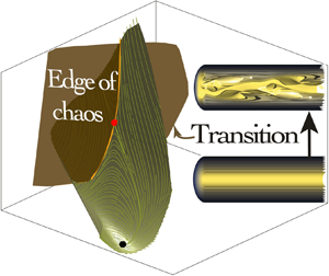
At the end of this two-step procedure, Kaszás & Haller (Reference Kaszás and Haller2023) have established a nonlinear manifold that links the hyperbolic anchor point of laminar Hagen–Poiseuille flow to a saddle point in the form of a lower-branch travelling-wave solution. This global representation of the reduced phase-space dynamics allows then the exploration of sections of the manifold that were not part of the training set. In other words, the SSM technique produces a predictive model of the phase-space dynamics within the accuracy of its polynomial approximation. Most importantly, it allows the computation of the edge manifold as the stable codimension-one manifold associated with the lower-branch travelling-wave solution. An illustration of the two-dimensional mixed-mode SSM is given in figure 1(a), taken from Kaszás & Haller (Reference Kaszás and Haller2023). The laminar state at $(J,K) = (0,0)$ (marked by a black symbol) represents Hagen–Poiseuille flow; the lower-branch travelling-wave solution is marked in red. The computed submanifold identifies the lower-branch solution as a saddle point, whose unstable directions connect to the laminar state and point towards the upper-branch solution. The same SSM also predicts a stable manifold associated with the identified saddle. The dynamics on the two-dimensional manifold, given via the second step of the SSM-technique, presents a clear and compelling picture of the global dynamics in the neighbourhoods of stable and unstable branches and along heteroclinic orbits.
Figure 1. (a) Phase-space trajectories from a SSM description of subcritical pipe-flow transition, expressed in a reduced $(J,K)$-phase space. (b) Initial conditions are chosen near the lower-branch travelling-wave solution and coloured according to their long-time fate: relaminarization (blue) or transition to turbulence (red).
Owing to the reduction to a two-dimensional phase space, the edge manifold is a simple curve, given by the stable direction of the lower-branch travelling-wave solution. It acts as a separatrix that divides the neighbourhood of the lower-branch solution into transitioning and relaminarizing trajectories and can be thought of as a low-dimensional representation of the full codimension-one edge-of-chaos manifold. To corroborate the influence of this separatrix over the transition behaviour in both the low-dimensional and high-dimensional space, Kaszás & Haller (Reference Kaszás and Haller2023) perform a numerical experiment where they seed initial conditions in a $\delta$-vicinity of the lower-branch solution, with some of the initial conditions falling on the ‘relaminarizing side’ of the predicted edge manifold and others starting on the ‘transitioning side’ (see figure 1b). Integrating these initial conditions in time, using direct numerical simulations (Willis Reference Willis2017), an accurate prediction as to their fate could be made based on the starting sector around the identified lower-branch saddle point in $(J,K)$-phase space. In figure 1(b), the initial conditions are coloured according to their long-time behaviour: red for initial conditions that approach the upper-branch solution; blue for initial conditions that decay towards the laminar (Hagen–Poiseuille) state. An excellent agreement between the ultimate long-term state and the initial starting position has been obtained, despite the exceedingly low-dimensional representation of the high-dimensional dynamics.
3. Future
The article by Kaszás & Haller (Reference Kaszás and Haller2023) constitutes a promising and encouraging step forward in the low-dimensional and accurate description of complex transition problems in wall-bounded shear flows. The application to pipe flow transition, a fundamental and well-studied subject, has resulted in an efficient and elegant representation of the edge manifold that captures dynamic features of the high-dimensional system reduced to a very low-dimensional manifold, without sacrificing any degree of predictive accuracy.
It has to be kept in mind, however, that the results obtained crucially rely on a novel and powerful data-driven technique, and any appraisal of the article by Kaszás & Haller (Reference Kaszás and Haller2023) must acknowledge not only the striking results in subcritical pipe flow transition, but also the tool that enabled them. A SSM reduction is certainly capable of equally impressive advances in other fields. This approach opens up new directions in the analysis of bistable and multistable configurations, such as fluid systems that are characterized by transitions between coexisting and competing states. In these pervasive systems, linearization about local equilibria and linear-tangent approximations yield limited results – or miss the pertinent dynamics (between the multiple quasisteady states) altogether. A phase-space perspective, combined with a manifold-extraction procedure, seems far more promising and appropriate, and SSM reduction, as demonstrated by Kaszás & Haller (Reference Kaszás and Haller2023), may be the tool for a more fitting analysis of nonlinearizable systems using data-driven techniques (see Cenedese et al. Reference Cenedese, Axås, Bäuerlein, Avila and Haller2022). The article by Kaszás & Haller (Reference Kaszás and Haller2023), presenting a confluence of a challenging application and a remarkable technique, has outlined the way ahead for future analyses of complex fluid systems.
In addition, the learned dynamics on the identified SSM can be augmented by forcing terms allowing, for example, a response analysis of the flow or the design of control strategies to manipulate the analysed configuration. This predictive property of the SSM reduction holds a rich array of opportunities that are waiting to be explored.


 $(J,K)$-phase space. (b) Initial conditions are chosen near the lower-branch travelling-wave solution and coloured according to their long-time fate: relaminarization (blue) or transition to turbulence (red).
 You have
Access
You have
Access
1. Introduction
Transition to turbulence has been a central field of study in fluid dynamics research since the pipe flow experiment of Osborne Reynolds in 1883 (Reynolds Reference Reynolds1883). Countless investigations have been motivated by this landmark experiment which distinguished laminar (or ‘direct’) from turbulent (or ‘sinuous’) fluid motion, gave us the Reynolds number as the governing parameter and brought about linear, and later nonlinear, stability studies for viscous, incompressible flows. Over more than the century that followed this experiment, progress on the transition problem came in the form of stability theory, low-disturbance-environment experiments, direct numerical simulations and low-dimensional modelling. Over the same century, advances in measurement techniques, the advent of supercomputers, and, more recently, the rise of machine learning, optimization and mathematical analysis have been instrumental in gathering a wealth of results that amount to a considerable, yet still incomplete, understanding of the transition process. Still, the importance of accurately predicting the laminar–turbulent transition, and thus the drag dynamics or heat transfer for high-speed flows, will ensure that transition research will maintain its central role in aerodynamic design and general fluid dynamics.
Among the most recent attempts to describe the transition process, a dynamical-systems perspective has emerged that describes the transition in phase space and brings to bear such concepts as equilibria and quasiequilibria, heteroclinic orbits, basins of attraction, strange attractors and separatrices. Within this framework, the flow evolves along, and is bound to, a manifold in high-dimensional phase space and the shear-flow transition is described as a subcritical bifurcation process between two states: the laminar (Hagen–Poiseuille) state and a chaotic turbulent (upper-branch) state. Facilitating the transition between these two states is a lower-branch state that acts as a saddle point in phase space and directs phase-space trajectories either towards the turbulent state or back to the laminar solution. This lower-branch state has been identified for pipe flow in the form of a travelling-wave solution by Pringle & Kerswell (Reference Pringle and Kerswell2007).
The subcritical nature of the pipe flow transition supports the coexistence of laminar and turbulent states over a range of Reynolds numbers (Duguet, Willis & Kerswell Reference Duguet, Willis and Kerswell2008), and the transition between them is governed by a set of trajectories that separates relaminarizing from transitioning solutions, referred to as the edge manifold or the edge of chaos (Skufca, Yorke & Eckhardt Reference Skufca, Yorke and Eckhardt2006). This edge manifold is a codimension-one manifold in phase space and acts as a conduit for initial perturbations about the laminar state to approach the lower-branch travelling-wave solution. The search for and analysis of this edge manifold has drawn a great deal of attention over the past two decades. However, it has been hampered by the fact that the subcritical nature of the shear-flow transition, the coexistence of multiple states and the link between them, renders linear analysis techniques ineffective as they fail to capture the dynamics far from their linearization points. Instead, a nonlinear description is necessary.
Over the past decade, a great many direct numerical simulations have been performed to locate and describe the edge manifold. These studies have tackled the high-dimensional phase space and employed bisection and bracketing techniques to gradually map out the edge of chaos and ultimately delineate the catchment basin of the laminar state from the one of the turbulent state via the attracting manifold of the lower-branch travelling-wave solution. In contrast to these efforts, the article by Kaszás & Haller (Reference Kaszás and Haller2023) applies the novel concept of invariant manifolds to formulate a low-dimensional, yet global representation of the phase-space dynamics, producing a parameterization that links the laminar equilibrium state to the lower-branch travelling-wave state and thus captures the edge manifold in the process. This representation arises from a data-driven, powerful technique (Haller & Ponsioen Reference Haller and Ponsioen2016; Haller et al. Reference Haller, Kaszás, Liu and Axås2023) known as spectral-submanifold (SSM) reduction, which plays a pivotal role in the findings reported in Kaszás & Haller (Reference Kaszás and Haller2023).
2. Overview
In the reduced description of Kaszás & Haller (Reference Kaszás and Haller2023) a set of observables is chosen that allows the projection of the full phase-space dynamics onto a restricted set of variables while still capturing the essential features of the transition dynamics. These variables have been chosen as the two-dimensional set $(J,K)$ with $J$ as the square root of the recentred energy input rate of the flow and $K$ as the square root of the normalized dissipation rate. The phase space expressed in these coordinates is thus two-dimensional. These reaction coordinates $(J,K)$ act as proxies for a high-dimensional dynamics, and a projective correspondence between the original high-dimensional phase space and the two-dimensional $(J,K)$-phase space is assumed.
The construction of the SSM proceeds in two steps, with the first step establishing the geometry of the manifold and the second step determining the dynamics along the identified manifold. The first step computes an orthogonal basis about an equilibrium state which is taken as the lower-branch travelling wave. This basis is then smoothly and nonlinearly extended using polynomials in $J$ and $K$ up to a prescribed degree. The basis manifold is thus deformed, starting from a linear tangent approximation, to accommodate nonlinear phase-space dynamics. The coefficients of this polynomial shaping are determined by minimizing the residual between the model predictions and the true observations given by a training data sequence. Crucially, the shaped manifold is required to connect the laminar state to the (reduced) lower-branch travelling-wave solution, hence linking the two equilibrium states. This requirement is included as an additional constraint in the optimization procedure. More precisely, tangency of the SSM, anchored to the lower-branch travelling-wave state, to both the single unstable and the slowest stable eigenvector of the lower-branch solution is enforced. The fact that the SSM connects to eigendirections of mixed stability categorizes it as a mixed-mode SSM (Haller et al. Reference Haller, Kaszás, Liu and Axås2023). Once the geometry of the manifold is established, in a second step, the training data is time-differenced and fed once more to an optimization routine to determine a second set of coefficients for the dynamics on the manifold. The description of the dynamics is again in terms of polynomials in $J$ and $K.$ Together with the geometry of the manifold, the SSM-technique has, in the end, produced an explicit representation of the latent-space dynamics, expressed in a low-dimensional $(J,K)$-phase space and learned from high-dimensional data.
At the end of this two-step procedure, Kaszás & Haller (Reference Kaszás and Haller2023) have established a nonlinear manifold that links the hyperbolic anchor point of laminar Hagen–Poiseuille flow to a saddle point in the form of a lower-branch travelling-wave solution. This global representation of the reduced phase-space dynamics allows then the exploration of sections of the manifold that were not part of the training set. In other words, the SSM technique produces a predictive model of the phase-space dynamics within the accuracy of its polynomial approximation. Most importantly, it allows the computation of the edge manifold as the stable codimension-one manifold associated with the lower-branch travelling-wave solution. An illustration of the two-dimensional mixed-mode SSM is given in figure 1(a), taken from Kaszás & Haller (Reference Kaszás and Haller2023). The laminar state at $(J,K) = (0,0)$ (marked by a black symbol) represents Hagen–Poiseuille flow; the lower-branch travelling-wave solution is marked in red. The computed submanifold identifies the lower-branch solution as a saddle point, whose unstable directions connect to the laminar state and point towards the upper-branch solution. The same SSM also predicts a stable manifold associated with the identified saddle. The dynamics on the two-dimensional manifold, given via the second step of the SSM-technique, presents a clear and compelling picture of the global dynamics in the neighbourhoods of stable and unstable branches and along heteroclinic orbits.
Figure 1. (a) Phase-space trajectories from a SSM description of subcritical pipe-flow transition, expressed in a reduced $(J,K)$-phase space. (b) Initial conditions are chosen near the lower-branch travelling-wave solution and coloured according to their long-time fate: relaminarization (blue) or transition to turbulence (red).
Owing to the reduction to a two-dimensional phase space, the edge manifold is a simple curve, given by the stable direction of the lower-branch travelling-wave solution. It acts as a separatrix that divides the neighbourhood of the lower-branch solution into transitioning and relaminarizing trajectories and can be thought of as a low-dimensional representation of the full codimension-one edge-of-chaos manifold. To corroborate the influence of this separatrix over the transition behaviour in both the low-dimensional and high-dimensional space, Kaszás & Haller (Reference Kaszás and Haller2023) perform a numerical experiment where they seed initial conditions in a $\delta$-vicinity of the lower-branch solution, with some of the initial conditions falling on the ‘relaminarizing side’ of the predicted edge manifold and others starting on the ‘transitioning side’ (see figure 1b). Integrating these initial conditions in time, using direct numerical simulations (Willis Reference Willis2017), an accurate prediction as to their fate could be made based on the starting sector around the identified lower-branch saddle point in $(J,K)$-phase space. In figure 1(b), the initial conditions are coloured according to their long-time behaviour: red for initial conditions that approach the upper-branch solution; blue for initial conditions that decay towards the laminar (Hagen–Poiseuille) state. An excellent agreement between the ultimate long-term state and the initial starting position has been obtained, despite the exceedingly low-dimensional representation of the high-dimensional dynamics.
3. Future
The article by Kaszás & Haller (Reference Kaszás and Haller2023) constitutes a promising and encouraging step forward in the low-dimensional and accurate description of complex transition problems in wall-bounded shear flows. The application to pipe flow transition, a fundamental and well-studied subject, has resulted in an efficient and elegant representation of the edge manifold that captures dynamic features of the high-dimensional system reduced to a very low-dimensional manifold, without sacrificing any degree of predictive accuracy.
It has to be kept in mind, however, that the results obtained crucially rely on a novel and powerful data-driven technique, and any appraisal of the article by Kaszás & Haller (Reference Kaszás and Haller2023) must acknowledge not only the striking results in subcritical pipe flow transition, but also the tool that enabled them. A SSM reduction is certainly capable of equally impressive advances in other fields. This approach opens up new directions in the analysis of bistable and multistable configurations, such as fluid systems that are characterized by transitions between coexisting and competing states. In these pervasive systems, linearization about local equilibria and linear-tangent approximations yield limited results – or miss the pertinent dynamics (between the multiple quasisteady states) altogether. A phase-space perspective, combined with a manifold-extraction procedure, seems far more promising and appropriate, and SSM reduction, as demonstrated by Kaszás & Haller (Reference Kaszás and Haller2023), may be the tool for a more fitting analysis of nonlinearizable systems using data-driven techniques (see Cenedese et al. Reference Cenedese, Axås, Bäuerlein, Avila and Haller2022). The article by Kaszás & Haller (Reference Kaszás and Haller2023), presenting a confluence of a challenging application and a remarkable technique, has outlined the way ahead for future analyses of complex fluid systems.
In addition, the learned dynamics on the identified SSM can be augmented by forcing terms allowing, for example, a response analysis of the flow or the design of control strategies to manipulate the analysed configuration. This predictive property of the SSM reduction holds a rich array of opportunities that are waiting to be explored.
Declaration of interests
The author report no conflict of interest.