


1 Introduction
When turbulence occurs in the presence of a stably stratified background gradient of density, it is common to observe the spontaneous formation of layers of well-mixed fluid separated by relatively sharp gradients or interfaces of density (Park, Whitehead & Gnanadeskian Reference Park, Whitehead and Gnanadeskian1994; Holford & Linden Reference Holford and Linden1999a ,Reference Holford and Linden b ; Oglethorpe, Caulfield & Woods Reference Oglethorpe, Caulfield and Woods2013; Falder, White & Caulfield Reference Falder, White and Caulfield2016; Leclercq et al. Reference Leclercq, Partridge, Augier, Caulfield, Dalziel and Linden2016b ; Thorpe Reference Thorpe2016). Such behaviour is of direct relevance to the atmosphere, oceans and various other environmental and industrial flows as these interfaces act as barriers to mixing and transport, and have a significant effect on the overall energetics of the flow.
Stratification also has a tendency to suppress vertical velocities due to the restoring force of gravity, thereby creating an inherent anisotropy in the flow when the stratification is large. Scaling arguments by Billant & Chomaz (Reference Billant and Chomaz2001) predict that such anisotropy occurs with a vertical ‘buoyancy’ length scale $l_{z}\sim U/N$
where
$l_{z}\sim U/N$
where $U$
is a typical horizontal velocity scale and
$U$
is a typical horizontal velocity scale and $N$
is the buoyancy or Brunt–Väisälä frequency. This scaling is observed ubiquitously in stratified flows exhibiting layers, although relatively few well-defined physical mechanisms are able to make direct contact with it.
$N$
is the buoyancy or Brunt–Väisälä frequency. This scaling is observed ubiquitously in stratified flows exhibiting layers, although relatively few well-defined physical mechanisms are able to make direct contact with it.
The motivation of this work is primarily to increase the connectivity between various approaches to the above problem of layer formation. The recent results presented in Lucas, Caulfield & Kerswell (Reference Lucas, Caulfield and Kerswell2017) (hereafter LCK) have demonstrated, using a triply periodic domain, that nonlinear exact coherent structures associated with layer formation can be traced through parameter space and connected to linear instabilities of a horizontally varying basic flow. Here we will consider a more physically realistic flow which has a base flow with horizontal shear. The flow is forced naturally by moving boundaries in a plane Couette flow (pCf) system with spanwise stratification (hereafter referred to as HSPC for horizontal stratified plane Couette).
This paper constitutes, along with the recent paper by Facchini et al. (Reference Facchini, Favier, Le Gal, Wang and Le Bars2018), the first exploration of the effect of spanwise stratification on plane Couette flow dynamics. Mainly considering flows at high Prandtl number, Facchini et al. (Reference Facchini, Favier, Le Gal, Wang and Le Bars2018) have shown that for the spanwise stratified version of plane Couette flow, a new linear instability appears when the geometry permits resonances between internal gravity waves. However, the instability only arises in geometries which allow the required critical relationship between vertical and streamwise wavelengths, given by the appropriately Doppler-shifted dispersion relationship. Therefore in many cases, and in particular at sufficiently low stratifications, a subcritical transition scenario comparable to unstratified pCf is observed. These two possible routes to turbulence make this flow geometry a particularly attractive one to investigate further the mechanisms by which stratification can affect turbulent flows, as well as identifying whether the initial (subcritical or supercritical) transition mechanisms leave a qualitatively identifiable imprint on the ensuing turbulent dynamics.
There is an increasing body of literature considering the similar configuration for (axially) stratified Taylor–Couette flow (Molemaker, McWilliams & Yavneh Reference Molemaker, McWilliams and Yavneh2001; Shalybkov & Rüdiger Reference Shalybkov and Rüdiger2005; Oglethorpe et al. Reference Oglethorpe, Caulfield and Woods2013; Leclercq, Nguyen & Kerswell Reference Leclercq, Nguyen and Kerswell2016a ; Leclercq et al. Reference Leclercq, Partridge, Augier, Caulfield, Dalziel and Linden2016b ; Park, Billant & Baik Reference Park, Billant and Baik2017; Park et al. Reference Park, Billant, Baik and Seo2018) from experimental, numerical and theoretical approaches. The primary focus for this flow has been the interplay between various instability mechanisms, in particular between the so-called centrifugal and stratorotational instabilities (Molemaker et al. Reference Molemaker, McWilliams and Yavneh2001; Shalybkov & Rüdiger Reference Shalybkov and Rüdiger2005; Leclercq et al. Reference Leclercq, Nguyen and Kerswell2016a ). In certain situations it is possible to observe the formation of layers, often confined near the walls, the source of which is the subject of continued debate. Part of the motivation of this work is to remove the effects of rotation and curvature from this system by taking the narrow-gap limit to try to uncover the universal, persistent features of such flows.
Also of interest is the comparison to the recently studied situation where the shear and stratification gradients are aligned. This case has been examined to study spatio-temporal dynamics, in particular the extent to which stratification can suppress turbulence and lead to relaminarisation (Deusebio, Caulfield & Taylor Reference Deusebio, Caulfield and Taylor2015; Taylor et al. Reference Taylor, Deusebio, Caulfield and Kerswell2016), irreversible mixing and layer robustness properties (Zhou, Taylor & Caulfield Reference Zhou, Taylor and Caulfield2017a ; Zhou et al. Reference Zhou, Taylor, Caulfield and Linden2017b ) and the effect of stratification on underlying exact coherent structures (Clever & Busse Reference Clever and Busse1992, Reference Clever, Busse, Egbers and Pfister2000; Deguchi Reference Deguchi2017; Olvera & Kerswell Reference Olvera and Kerswell2017).
In this paper we establish that, as in the vertically sheared case, only relatively weak stratification (in a sense which we make precise below) leads to suppression of the subcritical turbulence present in plane Couette flow, at least in flow geometries of aspect ratio $O(1{-}10)$
. Perhaps unsurprisingly, when the flow is linearly unstable to the instability identified by Facchini et al. (Reference Facchini, Favier, Le Gal, Wang and Le Bars2018), yet is still below the relaminarisation boundary, turbulent transition occurs supercritically. By considering flow geometries at similar parameters that can either admit or not this linear instability, we conclude that the supercritically triggered turbulent state is similar to the subcritically triggered turbulent state, namely having the characteristics of the self-sustaining process or wave–vortex interaction (SSP/VWI) mechanism (Hall & Smith Reference Hall and Smith1991; Waleffe Reference Waleffe1997; Hall & Sherwin Reference Hall and Sherwin2010). Furthermore, when the flow is linearly unstable, yet above the relaminarisation boundary, although perturbations saturate at finite amplitude, they remain relatively ordered, with only highly spatio-temporally intermittent ‘bursts’ of disordered motions.
$O(1{-}10)$
. Perhaps unsurprisingly, when the flow is linearly unstable to the instability identified by Facchini et al. (Reference Facchini, Favier, Le Gal, Wang and Le Bars2018), yet is still below the relaminarisation boundary, turbulent transition occurs supercritically. By considering flow geometries at similar parameters that can either admit or not this linear instability, we conclude that the supercritically triggered turbulent state is similar to the subcritically triggered turbulent state, namely having the characteristics of the self-sustaining process or wave–vortex interaction (SSP/VWI) mechanism (Hall & Smith Reference Hall and Smith1991; Waleffe Reference Waleffe1997; Hall & Sherwin Reference Hall and Sherwin2010). Furthermore, when the flow is linearly unstable, yet above the relaminarisation boundary, although perturbations saturate at finite amplitude, they remain relatively ordered, with only highly spatio-temporally intermittent ‘bursts’ of disordered motions.
In general, we observe that stratification always appears to have an effect on the dynamics, by altering the large-scale secondary flow patterns. These modified mean flows induce the formation of density layers near the walls which exhibit the familiar $U/N$
buoyancy scaling, although the physical mechanism leading to their formation is different from that underlying the previously identified ‘zig-zag’-like instabilities (Billant & Chomaz Reference Billant and Chomaz2000a
, LCK). At fixed Reynolds number, we demonstrate that the relaminarisation boundary as the stratification becomes relatively stronger corresponds to the intersection of this buoyancy scale of the secondary flow and the length scale associated with the spacing of the streaks. This implies that subcritical turbulence transition is controlled by a different competition of length scales compared to the wall-normal stratified case where Deusebio et al. (Reference Deusebio, Caulfield and Taylor2015) demonstrated that the competition between the Monin–Obukhov length scale and the (inner) viscous scale controls relaminarisation and intermittency.
$U/N$
buoyancy scaling, although the physical mechanism leading to their formation is different from that underlying the previously identified ‘zig-zag’-like instabilities (Billant & Chomaz Reference Billant and Chomaz2000a
, LCK). At fixed Reynolds number, we demonstrate that the relaminarisation boundary as the stratification becomes relatively stronger corresponds to the intersection of this buoyancy scale of the secondary flow and the length scale associated with the spacing of the streaks. This implies that subcritical turbulence transition is controlled by a different competition of length scales compared to the wall-normal stratified case where Deusebio et al. (Reference Deusebio, Caulfield and Taylor2015) demonstrated that the competition between the Monin–Obukhov length scale and the (inner) viscous scale controls relaminarisation and intermittency.
Interestingly, we find that for sufficiently large Reynolds numbers, the critical strength of stratification leading to relaminarisation is higher in the spanwise stratified case considered here than in the wall-normal stratified case of Deusebio et al. (Reference Deusebio, Caulfield and Taylor2015). This observation of turbulence ‘surviving’ at higher stratification is consistent with the commonly observed phenomenon that shear flows where the velocity gradient is orthogonal to the density gradient (usually referred to as ‘horizontal shear’) allow for stronger injection of perturbation kinetic energy from this shear into ensuing turbulent flows (Jacobitz & Sarkar Reference Jacobitz and Sarkar1998), than in flows with ‘vertical shear’ where the velocity and density gradients are parallel. Furthermore, although at higher Reynolds number in some appropriate flow geometries, turbulence can be triggered supercritically via the linear instability identified by Facchini et al. (Reference Facchini, Favier, Le Gal, Wang and Le Bars2018), rather than subcritically, the ultimate sustained turbulent attractor is, as expected, the same.
To illustrate these various issues and observations, the rest of this paper is organised as follows. Section 2 provides the formulation of the numerical simulation and defines the various parameters of interest. Section 3 presents the results of the numerical simulations conducted when the base flow is linearly stable, in particular discussing the formation of layers and their influence on relaminarisation. Section 4 considers linearly unstable flows and how the relaminarisation boundary affects the nonlinear dynamics. Finally, § 5 provides some further discussion and conclusions.
2 Formulation
We begin by considering the following version of the wall-forced, incompressible, Boussinesq equations
 $$\begin{eqnarray}\displaystyle & \displaystyle \frac{\unicode[STIX]{x2202}\boldsymbol{u}^{\ast }}{\unicode[STIX]{x2202}t^{\ast }}+\boldsymbol{u}^{\ast }\boldsymbol{\cdot }\unicode[STIX]{x1D6FB}^{\ast }\boldsymbol{u}^{\ast }+\frac{1}{\unicode[STIX]{x1D70C}_{0}}\unicode[STIX]{x1D6FB}^{\ast }p^{\ast }=\unicode[STIX]{x1D708}\unicode[STIX]{x1D6E5}^{\ast }\boldsymbol{u}^{\ast }-\frac{\unicode[STIX]{x1D70C}^{\ast }g}{\unicode[STIX]{x1D70C}_{0}}\hat{\boldsymbol{z}}, & \displaystyle\end{eqnarray}$$
 $$\begin{eqnarray}\displaystyle & \displaystyle \frac{\unicode[STIX]{x2202}\unicode[STIX]{x1D70C}^{\ast }}{\unicode[STIX]{x2202}t^{\ast }}+\boldsymbol{u}^{\ast }\boldsymbol{\cdot }\unicode[STIX]{x1D6FB}^{\ast }\unicode[STIX]{x1D70C}^{\ast }+\boldsymbol{u}^{\ast }\boldsymbol{\cdot }\unicode[STIX]{x1D6FB}^{\ast }\unicode[STIX]{x1D70C}_{B}=\unicode[STIX]{x1D705}\unicode[STIX]{x1D6E5}^{\ast }\unicode[STIX]{x1D70C}^{\ast }, & \displaystyle\end{eqnarray}$$
 $$\begin{eqnarray}\displaystyle & \unicode[STIX]{x1D6FB}^{\ast }\boldsymbol{\cdot }\boldsymbol{u}^{\ast }=0. & \displaystyle\end{eqnarray}$$
where $\boldsymbol{u}^{\ast }(x,y,z,t)=u^{\ast }\hat{\boldsymbol{x}}+v^{\ast }\hat{\boldsymbol{y}}+w^{\ast }\hat{\boldsymbol{z}}$
is the three-dimensional velocity field,
$\boldsymbol{u}^{\ast }(x,y,z,t)=u^{\ast }\hat{\boldsymbol{x}}+v^{\ast }\hat{\boldsymbol{y}}+w^{\ast }\hat{\boldsymbol{z}}$
is the three-dimensional velocity field, $\unicode[STIX]{x1D708}$
is the kinematic viscosity,
$\unicode[STIX]{x1D708}$
is the kinematic viscosity, $\unicode[STIX]{x1D705}$
is the molecular diffusivity,
$\unicode[STIX]{x1D705}$
is the molecular diffusivity, $p^{\ast }$
is the pressure,
$p^{\ast }$
is the pressure, $\unicode[STIX]{x1D70C}_{0}$
is an appropriate reference density and
$\unicode[STIX]{x1D70C}_{0}$
is an appropriate reference density and $\unicode[STIX]{x1D70C}^{\ast }(x,y,z,t)$
the varying part of the density away from the background linear density profile
$\unicode[STIX]{x1D70C}^{\ast }(x,y,z,t)$
the varying part of the density away from the background linear density profile $\unicode[STIX]{x1D70C}_{B}=-\unicode[STIX]{x1D6FD}z$
, i.e.
$\unicode[STIX]{x1D70C}_{B}=-\unicode[STIX]{x1D6FD}z$
, i.e. $\unicode[STIX]{x1D70C}_{total}=\unicode[STIX]{x1D70C}_{0}+\unicode[STIX]{x1D70C}_{B}(z)+\unicode[STIX]{x1D70C}^{\ast }(x,y,z,t)$
. We impose periodic boundary conditions in the streamwise,
$\unicode[STIX]{x1D70C}_{total}=\unicode[STIX]{x1D70C}_{0}+\unicode[STIX]{x1D70C}_{B}(z)+\unicode[STIX]{x1D70C}^{\ast }(x,y,z,t)$
. We impose periodic boundary conditions in the streamwise, $x$
, and spanwise,
$x$
, and spanwise, $z$
, directions with no-slip walls for
$z$
, directions with no-slip walls for $\boldsymbol{u}^{\ast }$
and no flux for
$\boldsymbol{u}^{\ast }$
and no flux for $\unicode[STIX]{x1D70C}^{\ast }$
in
$\unicode[STIX]{x1D70C}^{\ast }$
in $y$
:
$y$
:
 $$\begin{eqnarray}\boldsymbol{u}^{\ast }(x,y=-L_{y},z)=(-U_{y},0,0),\quad \boldsymbol{u}^{\ast }(x,y=L_{y},z)=(U_{y},0,0),\end{eqnarray}$$
 $$\begin{eqnarray}\left.\frac{\unicode[STIX]{x2202}\unicode[STIX]{x1D70C}^{\ast }}{\unicode[STIX]{x2202}y}\right|_{y=-L_{y}}=\left.\frac{\unicode[STIX]{x2202}\unicode[STIX]{x1D70C}^{\ast }}{\unicode[STIX]{x2202}y}\right|_{y=L_{y}}=0\end{eqnarray}$$
and consider domains $(x,y,z)\in [0,L_{x}]\times [-L_{y},L_{y}]\times [0,L_{z}]$
. Within this coordinate system, gravity may be thought of as pointing in the (negative) vertical direction, and the pCf induces horizontal shear, hence we refer to the flow as HSPC.
$(x,y,z)\in [0,L_{x}]\times [-L_{y},L_{y}]\times [0,L_{z}]$
. Within this coordinate system, gravity may be thought of as pointing in the (negative) vertical direction, and the pCf induces horizontal shear, hence we refer to the flow as HSPC.
The system is naturally non-dimensionalised using the characteristic length scale $L_{y}$
, characteristic time scale
$L_{y}$
, characteristic time scale $U_{y}/L_{y}$
and density gradient scale
$U_{y}/L_{y}$
and density gradient scale $\unicode[STIX]{x1D6FD}=-\unicode[STIX]{x1D735}\unicode[STIX]{x1D70C}_{B}\boldsymbol{\cdot }\hat{\boldsymbol{z}}$
to give
$\unicode[STIX]{x1D6FD}=-\unicode[STIX]{x1D735}\unicode[STIX]{x1D70C}_{B}\boldsymbol{\cdot }\hat{\boldsymbol{z}}$
to give
 $$\begin{eqnarray}\displaystyle & \displaystyle \frac{\unicode[STIX]{x2202}\boldsymbol{u}}{\unicode[STIX]{x2202}t}+\boldsymbol{u}\boldsymbol{\cdot }\unicode[STIX]{x1D735}\boldsymbol{u}+\unicode[STIX]{x1D735}p=\frac{1}{Re}\unicode[STIX]{x0394}\boldsymbol{u}-F_{h}^{-2}\unicode[STIX]{x1D70C}\hat{\boldsymbol{z}}, & \displaystyle\end{eqnarray}$$
 $$\begin{eqnarray}\displaystyle & \displaystyle \frac{\unicode[STIX]{x2202}\unicode[STIX]{x1D70C}}{\unicode[STIX]{x2202}t}+\boldsymbol{u}\boldsymbol{\cdot }\unicode[STIX]{x1D735}\unicode[STIX]{x1D70C}=w+\frac{1}{Re\,Pr}\unicode[STIX]{x0394}\unicode[STIX]{x1D70C}, & \displaystyle\end{eqnarray}$$
 $$\begin{eqnarray}\displaystyle & \unicode[STIX]{x1D735}\boldsymbol{\cdot }\boldsymbol{u}=0, & \displaystyle\end{eqnarray}$$
where we define the Reynolds number $Re$
, an appropriate background horizontal Froude number
$Re$
, an appropriate background horizontal Froude number $F_{h}$
, the Prandtl number
$F_{h}$
, the Prandtl number $Pr$
and buoyancy frequency
$Pr$
and buoyancy frequency $N$
as
$N$
as
 $$\begin{eqnarray}Re:=\frac{U_{y}L_{y}}{\unicode[STIX]{x1D708}},\quad F_{h}:=\frac{U_{y}}{NL_{y}},\quad Pr:=\frac{\unicode[STIX]{x1D708}}{\unicode[STIX]{x1D705}},\quad N^{2}:=\frac{g\unicode[STIX]{x1D6FD}}{\unicode[STIX]{x1D70C}_{0}}.\end{eqnarray}$$
We choose to use the (horizontal) Froude number $F_{h}$
as the appropriate measure of the relative strength of the background shear to the background stratification as this is exactly in the same form as the Froude number considered by Facchini et al. (Reference Facchini, Favier, Le Gal, Wang and Le Bars2018). For the flow considered by Deusebio et al. (Reference Deusebio, Caulfield and Taylor2015), where the shear and density gradient are parallel, the natural parameter is the bulk Richardson number
$F_{h}$
as the appropriate measure of the relative strength of the background shear to the background stratification as this is exactly in the same form as the Froude number considered by Facchini et al. (Reference Facchini, Favier, Le Gal, Wang and Le Bars2018). For the flow considered by Deusebio et al. (Reference Deusebio, Caulfield and Taylor2015), where the shear and density gradient are parallel, the natural parameter is the bulk Richardson number $Ri$
, which is mathematically equivalent, within this formulation, to the inverse square of the Froude number, i.e.
$Ri$
, which is mathematically equivalent, within this formulation, to the inverse square of the Froude number, i.e. $Ri\equiv F_{h}^{-2}$
. It must always be remembered that for the flow we are considering here, the stratification does not act directly against wall-normal motions, and so the conventional interpretation of a Richardson number (or equivalently the inverse square of a Froude number) as quantifying the relative significance of potential energy to kinetic energy in the background shear must be done with care, and in particular there is no a priori reason why large values of
$Ri\equiv F_{h}^{-2}$
. It must always be remembered that for the flow we are considering here, the stratification does not act directly against wall-normal motions, and so the conventional interpretation of a Richardson number (or equivalently the inverse square of a Froude number) as quantifying the relative significance of potential energy to kinetic energy in the background shear must be done with care, and in particular there is no a priori reason why large values of $Ri$
(or small values of
$Ri$
(or small values of $F_{h}$
) will lead to the flow being stable. However, it is reasonable to draw some analogies between the flow considered here and the flow considered in Deusebio et al. (Reference Deusebio, Caulfield and Taylor2015), as their parameter
$F_{h}$
) will lead to the flow being stable. However, it is reasonable to draw some analogies between the flow considered here and the flow considered in Deusebio et al. (Reference Deusebio, Caulfield and Taylor2015), as their parameter $Ri$
and our parameter
$Ri$
and our parameter $F_{h}$
are both ratios of the characteristic time scales associated with the background density and velocity distributions. Furthermore, as is apparent from the governing equations, it is the inverse square of the Froude number which quantifies the coupling between the density and velocity fields.
$F_{h}$
are both ratios of the characteristic time scales associated with the background density and velocity distributions. Furthermore, as is apparent from the governing equations, it is the inverse square of the Froude number which quantifies the coupling between the density and velocity fields.
To characterise the basic energetics of the flows we define
 $$\begin{eqnarray}{\mathcal{K}}:={\textstyle \frac{1}{2}}\langle |\boldsymbol{u}^{\prime }|^{2}\rangle _{V},\quad \unicode[STIX]{x1D716}:=\frac{1}{Re}\langle |\unicode[STIX]{x1D735}\boldsymbol{u}^{\prime }|^{2}\rangle _{V},\end{eqnarray}$$
 $$\begin{eqnarray}\unicode[STIX]{x1D712}:=\frac{1}{Pr\,Re}\langle |\unicode[STIX]{x1D735}\unicode[STIX]{x1D70C}|^{2}\rangle _{V},\quad u_{\unicode[STIX]{x1D70F}}:=\sqrt{\unicode[STIX]{x1D70F}_{w}/\unicode[STIX]{x1D70C}_{0}};\quad \unicode[STIX]{x1D70F}_{w}:=\left.\unicode[STIX]{x1D708}\frac{\unicode[STIX]{x2202}u}{\unicode[STIX]{x2202}y}\right|_{y=\pm 1},\end{eqnarray}$$
where $\boldsymbol{u}^{\prime }=\boldsymbol{u}-\langle \boldsymbol{u}\rangle _{x}$
is the fluctuation velocity,
$\boldsymbol{u}^{\prime }=\boldsymbol{u}-\langle \boldsymbol{u}\rangle _{x}$
is the fluctuation velocity, ${\mathcal{K}}$
is the turbulent kinetic energy,
${\mathcal{K}}$
is the turbulent kinetic energy, $\unicode[STIX]{x1D716}$
is the turbulent dissipation rate,
$\unicode[STIX]{x1D716}$
is the turbulent dissipation rate, $\unicode[STIX]{x1D712}$
is the dissipation rate of density variance and
$\unicode[STIX]{x1D712}$
is the dissipation rate of density variance and $u_{\unicode[STIX]{x1D70F}}$
is the friction velocity defined in terms of the wall shear stress
$u_{\unicode[STIX]{x1D70F}}$
is the friction velocity defined in terms of the wall shear stress $\unicode[STIX]{x1D70F}_{w}$
. In these definitions,
$\unicode[STIX]{x1D70F}_{w}$
. In these definitions, $\langle (\cdot )\rangle _{V}:=\iiint (\cdot )\,\text{d}x\,\text{d}y\,\text{d}z/(2L_{x}L_{z})$
denotes a volume average,
$\langle (\cdot )\rangle _{V}:=\iiint (\cdot )\,\text{d}x\,\text{d}y\,\text{d}z/(2L_{x}L_{z})$
denotes a volume average, $\langle (\cdot )\rangle _{x}:=\int (\cdot )\,\text{d}x/L_{x}$
denotes a streamwise average
$\langle (\cdot )\rangle _{x}:=\int (\cdot )\,\text{d}x/L_{x}$
denotes a streamwise average $\langle \cdot \rangle _{t}=[\int _{0}^{T}(\cdot )\,\text{d}t]/T$
denotes a time average, where
$\langle \cdot \rangle _{t}=[\int _{0}^{T}(\cdot )\,\text{d}t]/T$
denotes a time average, where $T$
is normally close to the full simulation time (having removed the initial transient spin-up from the initial condition).
$T$
is normally close to the full simulation time (having removed the initial transient spin-up from the initial condition).
We fix $Pr=1$
throughout and solve the equations numerically using the DIABLO direct numerical simulation (DNS) code (Taylor Reference Taylor2008) which is mixed pseudospectral in
$Pr=1$
throughout and solve the equations numerically using the DIABLO direct numerical simulation (DNS) code (Taylor Reference Taylor2008) which is mixed pseudospectral in $(x,z)$
with second-order finite difference in the wall-normal direction and uses fourth-order Runge–Kutta (for the nonlinear and buoyancy terms) and Crank–Nicolson (for the diffusion terms) time stepping. The resolution
$(x,z)$
with second-order finite difference in the wall-normal direction and uses fourth-order Runge–Kutta (for the nonlinear and buoyancy terms) and Crank–Nicolson (for the diffusion terms) time stepping. The resolution $(N_{x},N_{y},N_{z})$
is defined such that
$(N_{x},N_{y},N_{z})$
is defined such that $N_{x}$
and
$N_{x}$
and $N_{z}$
are the number of Fourier collocation points in each direction and
$N_{z}$
are the number of Fourier collocation points in each direction and $N_{y}$
the number of finite difference points which are clustered near the wall. Following Moin & Mahesh (Reference Moin and Mahesh1998) and Deusebio et al. (Reference Deusebio, Caulfield and Taylor2015), we maintain spatial convergence by ensuring that
$N_{y}$
the number of finite difference points which are clustered near the wall. Following Moin & Mahesh (Reference Moin and Mahesh1998) and Deusebio et al. (Reference Deusebio, Caulfield and Taylor2015), we maintain spatial convergence by ensuring that $\unicode[STIX]{x0394}x^{+}\lesssim 8$
,
$\unicode[STIX]{x0394}x^{+}\lesssim 8$
, $\unicode[STIX]{x0394}z^{+}\lesssim 4$
and
$\unicode[STIX]{x0394}z^{+}\lesssim 4$
and $y_{10}^{+}\lesssim 10$
where
$y_{10}^{+}\lesssim 10$
where $y_{10}^{+}$
is the tenth point from the wall and the ‘
$y_{10}^{+}$
is the tenth point from the wall and the ‘ $+$
’ superscript represents the usual viscous scaling
$+$
’ superscript represents the usual viscous scaling $l^{+}=u_{\unicode[STIX]{x1D70F}}l/\unicode[STIX]{x1D708}$
. The simulations to follow are initialised with a broad band uniform spectrum of perturbations having randomised phases with large enough amplitude (10–20 % of the wall velocity) to trigger (subcritically) sustained turbulence.
$l^{+}=u_{\unicode[STIX]{x1D70F}}l/\unicode[STIX]{x1D708}$
. The simulations to follow are initialised with a broad band uniform spectrum of perturbations having randomised phases with large enough amplitude (10–20 % of the wall velocity) to trigger (subcritically) sustained turbulence.
3 Direct numerical simulations: subcritical turbulence
We begin by presenting two sets of direct numerical simulations which were carried out to survey the $(Re,F_{h})$
parameter space near subcritical transition to sustained turbulence, with different choices of streamwise domain length. Table 1 outlines the parameters and some single point statistics. Figure 1(b) shows
$(Re,F_{h})$
parameter space near subcritical transition to sustained turbulence, with different choices of streamwise domain length. Table 1 outlines the parameters and some single point statistics. Figure 1(b) shows $\langle {\mathcal{K}}\rangle _{t}$
in
$\langle {\mathcal{K}}\rangle _{t}$
in $(Re,F_{h})$
space, indicating the laminar–turbulent boundary (note the relaminarised cases are not shown in table 1). We find that a similar picture to the vertically shearing case of Deusebio et al. (Reference Deusebio, Caulfield and Taylor2015) emerges in that only relatively weak stratification is required to shift the critical Reynolds number required for sustained turbulence, and that stratification reduces the overall turbulent kinetic energy of the flow. Comparing specific values, we note that with horizontal mean shear, larger stratifications for turbulent flows are achievable than for the vertical case for sufficiently high flow Reynolds numbers, as we also plot on the figure the curve associated with the formula derived using Monin–Obukhov theory which predicts the intermittency boundary well in
$(Re,F_{h})$
space, indicating the laminar–turbulent boundary (note the relaminarised cases are not shown in table 1). We find that a similar picture to the vertically shearing case of Deusebio et al. (Reference Deusebio, Caulfield and Taylor2015) emerges in that only relatively weak stratification is required to shift the critical Reynolds number required for sustained turbulence, and that stratification reduces the overall turbulent kinetic energy of the flow. Comparing specific values, we note that with horizontal mean shear, larger stratifications for turbulent flows are achievable than for the vertical case for sufficiently high flow Reynolds numbers, as we also plot on the figure the curve associated with the formula derived using Monin–Obukhov theory which predicts the intermittency boundary well in $Re{-}F_{h}$
space for (wall-normal) stratified plane Couette flow, as shown in figure 18 of Deusebio et al. (Reference Deusebio, Caulfield and Taylor2015). Although this curve actually delineates the onset of intermittency, as Deusebio et al. (Reference Deusebio, Caulfield and Taylor2015) show in their figure 18, it is also a good estimate of the boundary between flows exhibiting some turbulence and flows which completely relaminarise.
$Re{-}F_{h}$
space for (wall-normal) stratified plane Couette flow, as shown in figure 18 of Deusebio et al. (Reference Deusebio, Caulfield and Taylor2015). Although this curve actually delineates the onset of intermittency, as Deusebio et al. (Reference Deusebio, Caulfield and Taylor2015) show in their figure 18, it is also a good estimate of the boundary between flows exhibiting some turbulence and flows which completely relaminarise.

Figure 1. (a) Schematic showing the base flow and the background stratification for HSPC. (b) ( $Re$
,
$Re$
, $F_{h}^{-2}$
) parameter space from the DNS in table 1 coloured with turbulent kinetic energy
$F_{h}^{-2}$
) parameter space from the DNS in table 1 coloured with turbulent kinetic energy $\langle {\mathcal{K}}\rangle _{t}$
showing the sustenance of the turbulence, where black dots represent
$\langle {\mathcal{K}}\rangle _{t}$
showing the sustenance of the turbulence, where black dots represent $\langle {\mathcal{K}}\rangle _{t}=0$
where the flow has relaminarised. Symbols corresponds to the groups of table 1; circles have
$\langle {\mathcal{K}}\rangle _{t}=0$
where the flow has relaminarised. Symbols corresponds to the groups of table 1; circles have $L_{x}=4\unicode[STIX]{x03C0}$
, squares have
$L_{x}=4\unicode[STIX]{x03C0}$
, squares have $L_{x}=\unicode[STIX]{x03C0}$
and triangles the domains permitting the linear instability as discussed in § 4. The dashed blue line marks the theoretical model (using Monin–Obukhov theory) which predicts the intermittency boundary well for wall-normal stratified pCf as reported in Deusebio et al. (Reference Deusebio, Caulfield and Taylor2015). The bulk Richardson number
$L_{x}=\unicode[STIX]{x03C0}$
and triangles the domains permitting the linear instability as discussed in § 4. The dashed blue line marks the theoretical model (using Monin–Obukhov theory) which predicts the intermittency boundary well for wall-normal stratified pCf as reported in Deusebio et al. (Reference Deusebio, Caulfield and Taylor2015). The bulk Richardson number $Ri$
in this model is equated to
$Ri$
in this model is equated to $F_{h}^{-2}$
for ease of comparison. The grey shaded region denotes the region of parameter space where the flow relaminarises, while the green region approximately denotes the region where the flow (for some combination of streamwise and vertical wavenumbers) is prone to the primary linear instability identified by Facchini et al. (Reference Facchini, Favier, Le Gal, Wang and Le Bars2018). The dashed grey curve extends the relaminarisation boundary into the linearly unstable region, extrapolating the anticipated boundary now between linearly unstable, yet ordered dynamics, and sustained wall turbulence. A triangle at
$F_{h}^{-2}$
for ease of comparison. The grey shaded region denotes the region of parameter space where the flow relaminarises, while the green region approximately denotes the region where the flow (for some combination of streamwise and vertical wavenumbers) is prone to the primary linear instability identified by Facchini et al. (Reference Facchini, Favier, Le Gal, Wang and Le Bars2018). The dashed grey curve extends the relaminarisation boundary into the linearly unstable region, extrapolating the anticipated boundary now between linearly unstable, yet ordered dynamics, and sustained wall turbulence. A triangle at $Re=10\,000$
,
$Re=10\,000$
, $F_{h}^{-2}=0.7$
denotes the case where the flow is linearly unstable but the SSP/VWI mechanism is suppressed leading to qualitatively different (and non-turbulent) flows, as discussed in § 4.
$F_{h}^{-2}=0.7$
denotes the case where the flow is linearly unstable but the SSP/VWI mechanism is suppressed leading to qualitatively different (and non-turbulent) flows, as discussed in § 4.
Our runs probe as high as $Re=15\,000$
. In principle, such large Reynolds numbers may allow the consideration of (still turbulent) flows with large enough stratifications to potentially approach the so-called layered anisotropic stratified turbulence LAST regime (Brethouwer et al.
Reference Brethouwer, Billant, Lindborg and Chomaz2007; Falder et al.
Reference Falder, White and Caulfield2016). In the LAST regime, there is a clear separation between the Kolmogorov viscous microscale
$Re=15\,000$
. In principle, such large Reynolds numbers may allow the consideration of (still turbulent) flows with large enough stratifications to potentially approach the so-called layered anisotropic stratified turbulence LAST regime (Brethouwer et al.
Reference Brethouwer, Billant, Lindborg and Chomaz2007; Falder et al.
Reference Falder, White and Caulfield2016). In the LAST regime, there is a clear separation between the Kolmogorov viscous microscale $\unicode[STIX]{x1D702}$
, the Ozmidov scale
$\unicode[STIX]{x1D702}$
, the Ozmidov scale $l_{O}$
(i.e. the largest vertical scale which is not strongly affected by the background stratification) and the typical large buoyancy layering scale of the turbulent flow. This scale separation implies the existence of a highly anisotropic strongly stratified yet still turbulent flow for scales between this buoyancy layering scale and the Ozmidov scale, with essentially isotropic turbulence for scales between
$l_{O}$
(i.e. the largest vertical scale which is not strongly affected by the background stratification) and the typical large buoyancy layering scale of the turbulent flow. This scale separation implies the existence of a highly anisotropic strongly stratified yet still turbulent flow for scales between this buoyancy layering scale and the Ozmidov scale, with essentially isotropic turbulence for scales between $l_{O}$
and
$l_{O}$
and $\unicode[STIX]{x1D702}$
.
$\unicode[STIX]{x1D702}$
.
However, it is not at all clear that the LAST regime can be accessed in flows with wall forcing, as all previous numerical investigations of this regime have (to the authors’ knowledge) involved various numerical body-forcing protocols to ensure the maintenance of turbulent motions in sufficiently strongly stratified flows. However, our intention here is not to investigate any properties of this regime. Rather, we wish to investigate the effect of intermediate (spanwise) stratification on the underlying plane Couette flow dynamics, and also whether this flow geometry can remain turbulent at sufficiently strong stratifications to allow the possibility of transition towards the LAST regime. We discuss the emergent scale separation and the definitions and emergence of vertical length scales in the following section.
Furthermore, we have conducted a linear stability analysis of this flow (with $Pr=1$
) and as shown by the green shaded region, at sufficiently high
$Pr=1$
) and as shown by the green shaded region, at sufficiently high $Re$
and small
$Re$
and small $F_{h}$
, the flow is linearly unstable (provided of course that the unstable vertical and streamwise wavelengths of the instability can ‘fit’ into the chosen computational domain) and so the apparent suppression of the subcritical route to turbulence no longer precludes the possibility of turbulence being sustained. This linear instability is the analogous instability (for flows with unit Prandtl number) to the instability identified by Facchini et al. (Reference Facchini, Favier, Le Gal, Wang and Le Bars2018) at infinite Schmidt number.
$F_{h}$
, the flow is linearly unstable (provided of course that the unstable vertical and streamwise wavelengths of the instability can ‘fit’ into the chosen computational domain) and so the apparent suppression of the subcritical route to turbulence no longer precludes the possibility of turbulence being sustained. This linear instability is the analogous instability (for flows with unit Prandtl number) to the instability identified by Facchini et al. (Reference Facchini, Favier, Le Gal, Wang and Le Bars2018) at infinite Schmidt number.
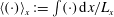
Figure 2 shows some typical flow field snapshots at $Re=5000$
and
$Re=5000$
and $F_{h}^{-2}=0.1$
, which is near to the largest possible stratification possible at this Reynolds number for which subcritically triggered turbulence can be sustained. At first inspection there appears to be little obvious influence of stratification on the typical plane Couette flow dynamics, as we still observe streaky flow, with streamwise waves propagating along the streaks.
$F_{h}^{-2}=0.1$
, which is near to the largest possible stratification possible at this Reynolds number for which subcritically triggered turbulence can be sustained. At first inspection there appears to be little obvious influence of stratification on the typical plane Couette flow dynamics, as we still observe streaky flow, with streamwise waves propagating along the streaks.
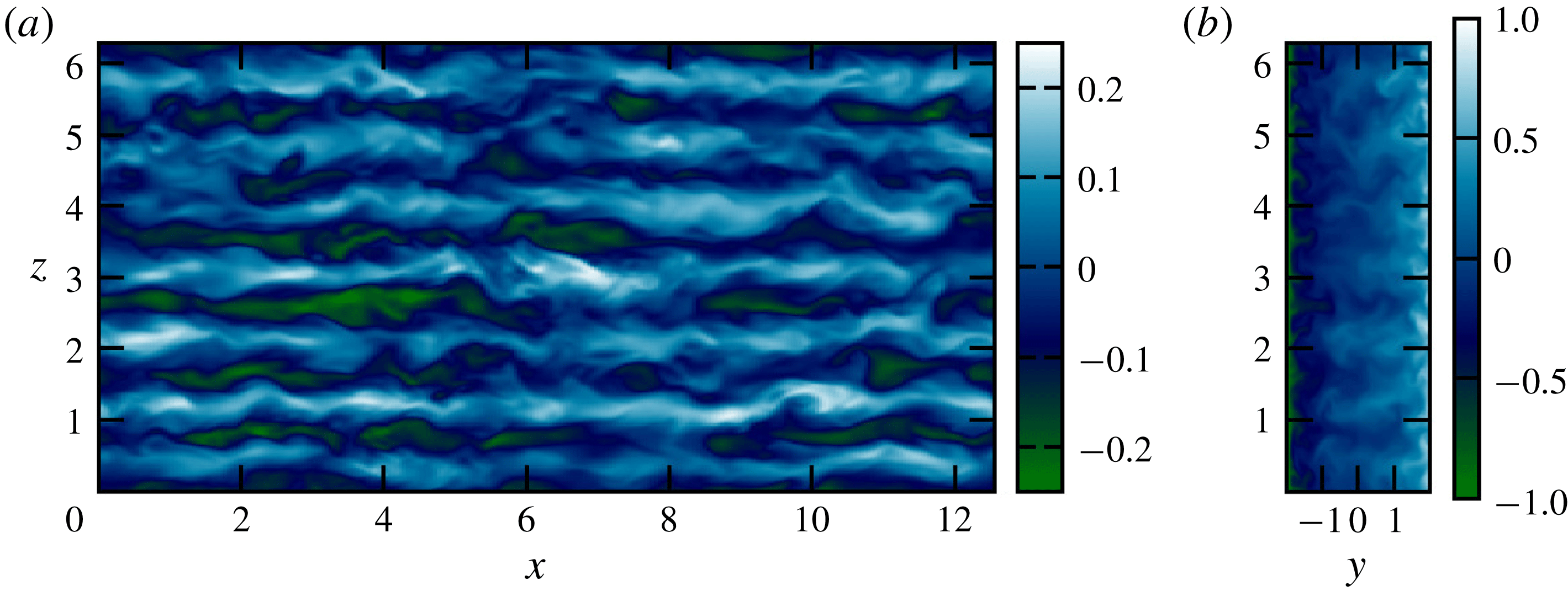
Figure 2. Streamwise velocity, $u$
, for the case
$u$
, for the case $Re=5000$
,
$Re=5000$
, $F_{h}^{-2}=0.1$
,
$F_{h}^{-2}=0.1$
, $Pr=1$
,
$Pr=1$
, $L_{x}=4\unicode[STIX]{x03C0}$
,
$L_{x}=4\unicode[STIX]{x03C0}$
, $L_{z}=2\unicode[STIX]{x03C0}$
from set 1 of DNS in table 1. Left panel shows the flow at the mid-gap
$L_{z}=2\unicode[STIX]{x03C0}$
from set 1 of DNS in table 1. Left panel shows the flow at the mid-gap $y=0$
and the right panel shows the flow for
$y=0$
and the right panel shows the flow for $x=0$
. Seen are the streaks of high/low speed fluid which have been lifted from near the walls by streamwise rolls, as one expects in plane Couette flow. In these images there is no discernible effect of stratification on the dynamics.
$x=0$
. Seen are the streaks of high/low speed fluid which have been lifted from near the walls by streamwise rolls, as one expects in plane Couette flow. In these images there is no discernible effect of stratification on the dynamics.
Table 1. Some DNS diagnostics. Top group has $L_{x}=4\unicode[STIX]{x03C0}$
,
$L_{x}=4\unicode[STIX]{x03C0}$
, $L_{z}=2\unicode[STIX]{x03C0}$
,
$L_{z}=2\unicode[STIX]{x03C0}$
, $N_{x}=256$
,
$N_{x}=256$
, $N_{z}=256$
,
$N_{z}=256$
, $N_{y}=129$
. Middle group has
$N_{y}=129$
. Middle group has $L_{x}=\unicode[STIX]{x03C0}$
,
$L_{x}=\unicode[STIX]{x03C0}$
, $L_{z}=2\unicode[STIX]{x03C0}$
, with
$L_{z}=2\unicode[STIX]{x03C0}$
, with $N_{x}=64$
, apart from
$N_{x}=64$
, apart from $Re=10\,000$
and 15 000 which required
$Re=10\,000$
and 15 000 which required $N_{x}=128$
,
$N_{x}=128$
, $N_{z}=512$
and
$N_{z}=512$
and $N_{y}=161$
. Bottom group is the two linearly unstable cases
$N_{y}=161$
. Bottom group is the two linearly unstable cases $F_{h}^{-2}=0.2$
having
$F_{h}^{-2}=0.2$
having $L_{x}=16.5$
,
$L_{x}=16.5$
, $L_{z}=5.8$
and
$L_{z}=5.8$
and $F_{h}^{-2}=0.7$
having
$F_{h}^{-2}=0.7$
having $L_{x}=12$
,
$L_{x}=12$
, $L_{z}=4$
. All have
$L_{z}=4$
. All have $Pr=1$
. Averages in time are taken after the initial transient, the time averaging window is given as
$Pr=1$
. Averages in time are taken after the initial transient, the time averaging window is given as $T$
in the table. The time averaging window for the linearly unstable case
$T$
in the table. The time averaging window for the linearly unstable case $Re=10\,000$
,
$Re=10\,000$
, $F_{h}^{-2}=0.2$
is taken once sustained wall turbulence is reached for comparison to the linearly stable values.
$F_{h}^{-2}=0.2$
is taken once sustained wall turbulence is reached for comparison to the linearly stable values. $Re_{B}=\unicode[STIX]{x1D716}\,Re\,F_{h}^{2}$
,
$Re_{B}=\unicode[STIX]{x1D716}\,Re\,F_{h}^{2}$
, $Fr=\unicode[STIX]{x1D716}F_{h}/(u_{rms}^{2})$
,
$Fr=\unicode[STIX]{x1D716}F_{h}/(u_{rms}^{2})$
, $l_{O}=\sqrt{\unicode[STIX]{x1D716}F_{h}^{3}}$
,
$l_{O}=\sqrt{\unicode[STIX]{x1D716}F_{h}^{3}}$
, $Re_{\unicode[STIX]{x1D70F}}=L_{y}u_{\unicode[STIX]{x1D70F}}/\unicode[STIX]{x1D708}$
,
$Re_{\unicode[STIX]{x1D70F}}=L_{y}u_{\unicode[STIX]{x1D70F}}/\unicode[STIX]{x1D708}$
, $u_{rms}^{2}=\langle u^{\prime 2}\rangle _{V}$
with
$u_{rms}^{2}=\langle u^{\prime 2}\rangle _{V}$
with $l_{z}$
computed as discussed in § 3.1.
$l_{z}$
computed as discussed in § 3.1.

3.1 Layers
Despite the apparent weak dependence of the flow on the stratification, some differences can be observed. Figure 3 shows spatio-temporal diagrams of the perturbation density $\unicode[STIX]{x1D70C}$
(a,b) and
$\unicode[STIX]{x1D70C}$
(a,b) and $\unicode[STIX]{x1D70C}_{tot}$
(c,d) in
$\unicode[STIX]{x1D70C}_{tot}$
(c,d) in $(z,t)$
-planes at fixed
$(z,t)$
-planes at fixed $x$
and
$x$
and $y$
for the case
$y$
for the case $Re=5000$
,
$Re=5000$
, $F_{h}^{-2}=0.1$
,
$F_{h}^{-2}=0.1$
, $L_{x}=4\unicode[STIX]{x03C0}$
,
$L_{x}=4\unicode[STIX]{x03C0}$
, $L_{z}=2\unicode[STIX]{x03C0}$
. We show
$L_{z}=2\unicode[STIX]{x03C0}$
. We show $x=\unicode[STIX]{x03C0}$
and two
$x=\unicode[STIX]{x03C0}$
and two $y$
locations:
$y$
locations: $y=-0.98$
, i.e. near wall; and
$y=-0.98$
, i.e. near wall; and $y=0$
, mid-gap. The near-wall profiles clearly show the spontaneous formation of layers of alternately stronger and weaker stratification which are robust in time. By contrast, the flow in the centre of the channel is uniformly stratified with broadly isotropic fluctuations.
$y=0$
, mid-gap. The near-wall profiles clearly show the spontaneous formation of layers of alternately stronger and weaker stratification which are robust in time. By contrast, the flow in the centre of the channel is uniformly stratified with broadly isotropic fluctuations.

Figure 3. Spatio-temporal diagram in $(z,t)$
for profiles of density for
$(z,t)$
for profiles of density for $x=L_{x}/2$
and two
$x=L_{x}/2$
and two $y$
locations: near wall
$y$
locations: near wall $y=-0.98$
(a,c) and mid-gap
$y=-0.98$
(a,c) and mid-gap $y=0$
(b,d), for the case
$y=0$
(b,d), for the case $Re=5000$
,
$Re=5000$
, $F_{h}^{-2}=0.1$
,
$F_{h}^{-2}=0.1$
, $Pr=1$
,
$Pr=1$
, $L_{x}=4\unicode[STIX]{x03C0}$
,
$L_{x}=4\unicode[STIX]{x03C0}$
, $L_{z}=2\unicode[STIX]{x03C0}$
from set 1 of DNS in table 1. The top panels show the perturbation density
$L_{z}=2\unicode[STIX]{x03C0}$
from set 1 of DNS in table 1. The top panels show the perturbation density $\unicode[STIX]{x1D70C}$
in red/yellow, while the bottom panels show the total density
$\unicode[STIX]{x1D70C}$
in red/yellow, while the bottom panels show the total density $\unicode[STIX]{x1D70C}_{tot}=\unicode[STIX]{x1D70C}-z$
in grey scale. Note that layers are visible near the wall but there is only well-mixed fluid in the mid-channel.
$\unicode[STIX]{x1D70C}_{tot}=\unicode[STIX]{x1D70C}-z$
in grey scale. Note that layers are visible near the wall but there is only well-mixed fluid in the mid-channel.
Given the robustness in time of the near-wall structures, in figure 4 we plot the time- and streamwise-averaged densities in a $(y,z)$
-plane i.e.
$(y,z)$
-plane i.e. $\langle \unicode[STIX]{x1D70C}\rangle _{xt}$
for this case and several others from table 1. As
$\langle \unicode[STIX]{x1D70C}\rangle _{xt}$
for this case and several others from table 1. As $Re$
and
$Re$
and $F_{h}^{-2}$
are increased, coherent layers are observed, offset across the gap, and with decreasing vertical scale. Associated with this layering is a coherent pattern in the mean flows. Relatively large-scale flattened streamwise vortices develop with enhanced density gradients located between them, near the walls.
$F_{h}^{-2}$
are increased, coherent layers are observed, offset across the gap, and with decreasing vertical scale. Associated with this layering is a coherent pattern in the mean flows. Relatively large-scale flattened streamwise vortices develop with enhanced density gradients located between them, near the walls.

Figure 4. Streamwise- and time-averaged perturbation density $\langle \unicode[STIX]{x1D70C}\rangle _{x,t}$
for 4 cases from set 1 of DNS in table 1 as labelled. Notice the layers near the walls which are offset from each other across the gap.
$\langle \unicode[STIX]{x1D70C}\rangle _{x,t}$
for 4 cases from set 1 of DNS in table 1 as labelled. Notice the layers near the walls which are offset from each other across the gap.
Considering again the case $Re=5000$
,
$Re=5000$
, $F_{h}^{-2}=0.1$
,
$F_{h}^{-2}=0.1$
, $Pr=1$
and
$Pr=1$
and $L_{x}=4\unicode[STIX]{x03C0}$
and
$L_{x}=4\unicode[STIX]{x03C0}$
and $L_{z}=2\unicode[STIX]{x03C0}$
, figure 5 shows the streamwise- and time-averaged velocity components of the mean flow. The apparent vortical structure leads to vertical motions and hence buoyancy fluxes localised near the walls and an associated ‘zig-zag’ pattern in the streamwise velocity perturbation. This flow structure bears some resemblance to the exact coherent structures discussed in LCK as alternating spanwise velocities once again redistribute the background shear. A difference in this case is that the wall confinement causes the streamlines to form closed loops rather than penetrate through the periodic boundary as in LCK.
$L_{z}=2\unicode[STIX]{x03C0}$
, figure 5 shows the streamwise- and time-averaged velocity components of the mean flow. The apparent vortical structure leads to vertical motions and hence buoyancy fluxes localised near the walls and an associated ‘zig-zag’ pattern in the streamwise velocity perturbation. This flow structure bears some resemblance to the exact coherent structures discussed in LCK as alternating spanwise velocities once again redistribute the background shear. A difference in this case is that the wall confinement causes the streamlines to form closed loops rather than penetrate through the periodic boundary as in LCK.

Figure 5. Streamwise- and time-averaged total velocities $\langle \boldsymbol{u}\rangle _{xt}-y\hat{\boldsymbol{x}}$
for
$\langle \boldsymbol{u}\rangle _{xt}-y\hat{\boldsymbol{x}}$
for $Re=5000$ $F_{h}^{-2}=0.1$
,
$F_{h}^{-2}=0.1$
, $Pr=1$
,
$Pr=1$
, $L_{x}=4\unicode[STIX]{x03C0}$
,
$L_{x}=4\unicode[STIX]{x03C0}$
, $L_{z}=2\unicode[STIX]{x03C0}$
from set 1 of DNS in table 1. Streamwise vortices emerge as a coherent structure coupled to the density layering.
$L_{z}=2\unicode[STIX]{x03C0}$
from set 1 of DNS in table 1. Streamwise vortices emerge as a coherent structure coupled to the density layering.
There is also some similarity to the linear modes discovered in this system by Facchini et al. (Reference Facchini, Favier, Le Gal, Wang and Le Bars2018) insofar as there are density perturbations concentrated near the walls. However the length scales and driving mechanisms for these near-wall perturbations are completely different as can be seen in § 4, and so it may well be that the similarity is merely coincidental. At the largest Reynolds number and stratification considered there is some indication of an additional modulation to this layering pattern, the rightmost panel of figure 4 showing an approximately mode 3 structure on top of the much finer near-wall layers. We now seek to clarify the underlying mechanism for forming this persistent large-scale flow, and also to investigate how it influences the overall flow dynamics.
Having established that this large-scale structure is streamwise invariant in the relatively long streamwise domain $L_{x}=4\unicode[STIX]{x03C0}$
, i.e. in the averages of figure 5, we study flows with higher
$L_{x}=4\unicode[STIX]{x03C0}$
, i.e. in the averages of figure 5, we study flows with higher $Re$
and fixed
$Re$
and fixed $Re=5000$
with variable
$Re=5000$
with variable $F_{h}^{-2}$
in a shortened domain
$F_{h}^{-2}$
in a shortened domain $L_{x}=\unicode[STIX]{x03C0}$
to reduce the computational expense. These are shown in the second set of results in table 1. Note that even the least energetic of these cases has
$L_{x}=\unicode[STIX]{x03C0}$
to reduce the computational expense. These are shown in the second set of results in table 1. Note that even the least energetic of these cases has $Re_{\unicode[STIX]{x1D70F}}\approx 190$
corresponding to
$Re_{\unicode[STIX]{x1D70F}}\approx 190$
corresponding to $L_{x}^{+}\approx 600$
in viscous units, which should be comfortably above the minimal distance (Jimènez & Moin Reference Jimènez and Moin1991).
$L_{x}^{+}\approx 600$
in viscous units, which should be comfortably above the minimal distance (Jimènez & Moin Reference Jimènez and Moin1991).
Insight into the properties of these large-scale structures is gained by considering the limit $F_{h}\rightarrow \infty$
. In unstratified plane Couette flow, streamwise-invariant large-scale structures are known to exist at larger Reynolds number as weak secondary flows (Papavassiliou & Hanratty Reference Papavassiliou and Hanratty1997; Toh & Itano Reference Toh and Itano2005; Tsukahara, Kawamura & Shingai Reference Tsukahara, Kawamura and Shingai2006). Figure 6 shows snapshots of streamwise-averaged wall-normal velocity
$F_{h}\rightarrow \infty$
. In unstratified plane Couette flow, streamwise-invariant large-scale structures are known to exist at larger Reynolds number as weak secondary flows (Papavassiliou & Hanratty Reference Papavassiliou and Hanratty1997; Toh & Itano Reference Toh and Itano2005; Tsukahara, Kawamura & Shingai Reference Tsukahara, Kawamura and Shingai2006). Figure 6 shows snapshots of streamwise-averaged wall-normal velocity $\langle v\rangle _{x}$
for
$\langle v\rangle _{x}$
for $F_{h}^{-2}=0$
, 0.05 and 0.1 for
$F_{h}^{-2}=0$
, 0.05 and 0.1 for $Re=5000$
, which shows this large-scale structure in the unstratified case and the reduction in the vertical length scale of this structure as
$Re=5000$
, which shows this large-scale structure in the unstratified case and the reduction in the vertical length scale of this structure as $F_{h}$
decreases. These secondary streamwise rolls have been understood as essentially a large-scale condensate of an inverse cascade of quasi-two-dimensional streamwise vorticity. These structures are mostly inviscid, except near the walls and therefore require only relatively small energy flux to maintain them. A self-sustenance between the Reynolds stresses of the turbulence and the large-scale secondary flow allows the structure to persist in space and time.
$F_{h}$
decreases. These secondary streamwise rolls have been understood as essentially a large-scale condensate of an inverse cascade of quasi-two-dimensional streamwise vorticity. These structures are mostly inviscid, except near the walls and therefore require only relatively small energy flux to maintain them. A self-sustenance between the Reynolds stresses of the turbulence and the large-scale secondary flow allows the structure to persist in space and time.

Figure 6. Streamwise-averaged wall-normal velocity $\langle v\rangle _{x}$
for
$\langle v\rangle _{x}$
for $Re=5000$
,
$Re=5000$
, $Pr=1$
,
$Pr=1$
, $L_{x}=\unicode[STIX]{x03C0}$
,
$L_{x}=\unicode[STIX]{x03C0}$
, $L_{z}=2\unicode[STIX]{x03C0}$
for
$L_{z}=2\unicode[STIX]{x03C0}$
for $F_{h}^{-2}=0$
,
$F_{h}^{-2}=0$
, $F_{h}^{-2}=0.05$
and
$F_{h}^{-2}=0.05$
and $F_{h}^{-2}=0.1$
from DNS in table 1. The large-scale flow observed in unstratified plane Couette flow is shown in the leftmost panel, with the middle and right panels showing how stratification confines the secondary flow to a shallower vertical scale, decreasing with decreasing
$F_{h}^{-2}=0.1$
from DNS in table 1. The large-scale flow observed in unstratified plane Couette flow is shown in the leftmost panel, with the middle and right panels showing how stratification confines the secondary flow to a shallower vertical scale, decreasing with decreasing $F_{h}$
.
$F_{h}$
.
Due to their large scales, in the vertical in particular, these are the first coherent structures to feel the effect of stratification. As $F_{h}$
is decreased, this large-scale flow becomes constrained in the vertical,
$F_{h}$
is decreased, this large-scale flow becomes constrained in the vertical, $z$
, direction by the vertical buoyancy scale
$z$
, direction by the vertical buoyancy scale $l_{z}$
. The buoyancy length scale is commonly observed to scale as
$l_{z}$
. The buoyancy length scale is commonly observed to scale as $l_{z}\sim U/N$
(where
$l_{z}\sim U/N$
(where $U$
is a typical horizontal velocity scale) which has been predicted by scaling arguments of the governing equations Billant & Chomaz (Reference Billant and Chomaz2001) and also by linear instabilities (Billant & Chomaz (Reference Billant and Chomaz2001), LCK). Here we also observe this characteristic
$U$
is a typical horizontal velocity scale) which has been predicted by scaling arguments of the governing equations Billant & Chomaz (Reference Billant and Chomaz2001) and also by linear instabilities (Billant & Chomaz (Reference Billant and Chomaz2001), LCK). Here we also observe this characteristic $U/N$
scaling as shown in figure 7, where we have estimated
$U/N$
scaling as shown in figure 7, where we have estimated $l_{z}$
using a wavenumber centroid method on the spectra of
$l_{z}$
using a wavenumber centroid method on the spectra of $\langle v\rangle _{x,y,t}$
similar to the approach described in LCK, and chosen
$\langle v\rangle _{x,y,t}$
similar to the approach described in LCK, and chosen $U=v_{rms}$
.
$U=v_{rms}$
.
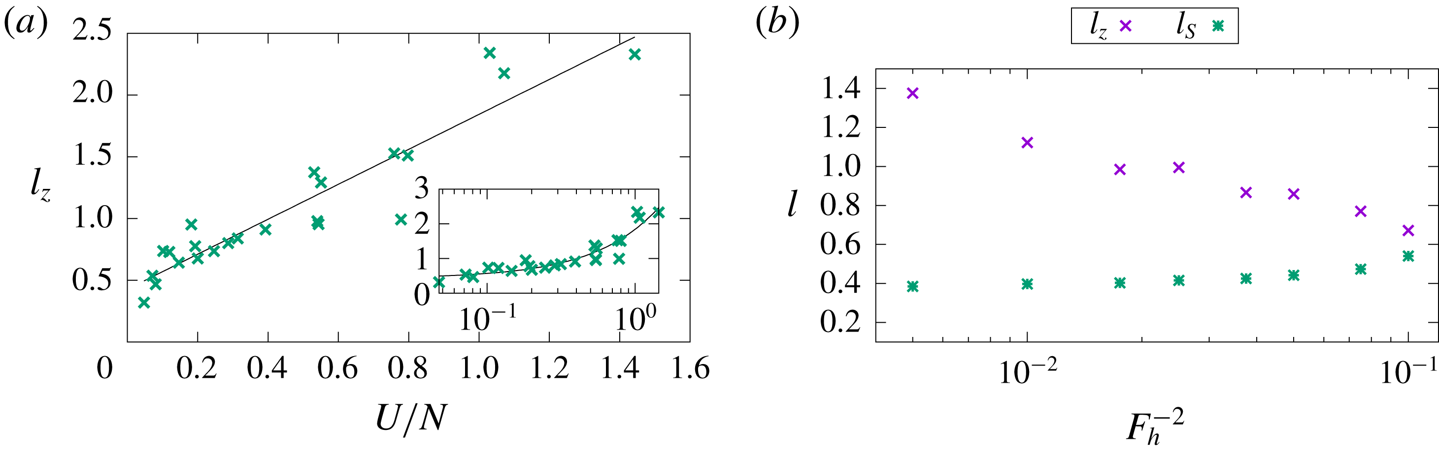
Figure 7. (a) Estimate of the vertical length scale of the mean streamwise roll, computed by a centroid of the Fourier transform of mean wall-normal velocity, plotted against an estimate of $U/N$
where
$U/N$
where $U\equiv v_{rms}$
and
$U\equiv v_{rms}$
and $N=F_{h}^{-1}$
. A linear fit is shown where
$N=F_{h}^{-1}$
. A linear fit is shown where $l_{z}=1.44U/N+0.39$
and data are given from all cases in table 1. Inset shows the same plotted with
$l_{z}=1.44U/N+0.39$
and data are given from all cases in table 1. Inset shows the same plotted with $U/N$
on a log axis to better show the cluster of points for
$U/N$
on a log axis to better show the cluster of points for $U/N<0.4$
. (b) Vertical length scales against
$U/N<0.4$
. (b) Vertical length scales against $F_{h}^{-2}$
for the case of fixed
$F_{h}^{-2}$
for the case of fixed $Re=5000$
from the second set of DNS in table 1.
$Re=5000$
from the second set of DNS in table 1. $l_{z}$
is given as in the left plot, along with
$l_{z}$
is given as in the left plot, along with $l_{S}=100\unicode[STIX]{x1D708}/u_{\unicode[STIX]{x1D70F}}$
. Decreasing
$l_{S}=100\unicode[STIX]{x1D708}/u_{\unicode[STIX]{x1D70F}}$
. Decreasing $F_{h}$
beyond the values given here results in relaminarisation of this subcritically triggered turbulent flow, which may be interpreted as occurring due to the intersection of the buoyancy scale with the streak spacing and subsequent disruption of the SSP/VWI mechanism by stratification.
$F_{h}$
beyond the values given here results in relaminarisation of this subcritically triggered turbulent flow, which may be interpreted as occurring due to the intersection of the buoyancy scale with the streak spacing and subsequent disruption of the SSP/VWI mechanism by stratification.
3.2 Relaminarisation
This interpretation of the layering and influence of the buoyancy scale on this system allows for further interpretation of the relaminarisation boundary. The next largest spanwise length scale in pCf dynamics is the inner streak spacing. This spacing has been established as $l_{S}=100\unicode[STIX]{x1D708}/u_{\unicode[STIX]{x1D70F}}$
(see e.g. Kline et al. (Reference Kline, Reynolds, Schraub and Runstadler1967), Kim, Moin & Moser (Reference Kim, Moin and Moser1987), Hamilton, Kim & Waleffe (Reference Hamilton, Kim and Waleffe1995)). By examining the case of fixed
$l_{S}=100\unicode[STIX]{x1D708}/u_{\unicode[STIX]{x1D70F}}$
(see e.g. Kline et al. (Reference Kline, Reynolds, Schraub and Runstadler1967), Kim, Moin & Moser (Reference Kim, Moin and Moser1987), Hamilton, Kim & Waleffe (Reference Hamilton, Kim and Waleffe1995)). By examining the case of fixed $Re=5000$
and varying only
$Re=5000$
and varying only $F_{h}$
we plot in figure 7 the buoyancy length scale
$F_{h}$
we plot in figure 7 the buoyancy length scale $l_{z}$
and the streak spacing
$l_{z}$
and the streak spacing $l_{S}$
. As
$l_{S}$
. As $F_{h}$
is decreased the two length scales become closer in value, and their intersection represents the relaminarisation point with respect to
$F_{h}$
is decreased the two length scales become closer in value, and their intersection represents the relaminarisation point with respect to $F_{h}$
at this
$F_{h}$
at this $Re$
.
$Re$
.
To analyse this scale convergence more carefully, we plot in figure 8 the spanwise spectra with $y$
of the normalised mean streamwise velocity
$y$
of the normalised mean streamwise velocity $\hat{U} ^{+}=\langle \hat{u} \rangle _{t}/u_{\unicode[STIX]{x1D70F}}$
(where
$\hat{U} ^{+}=\langle \hat{u} \rangle _{t}/u_{\unicode[STIX]{x1D70F}}$
(where $\hat{.}$
denotes the Fourier transform) for streamwise wavenumber
$\hat{.}$
denotes the Fourier transform) for streamwise wavenumber $k_{x}=2\unicode[STIX]{x03C0}/L_{x}$
. This choice is made to pick out the signature of the largest-scale streamwise mean flow and the near-wall fluctuations. For relatively large
$k_{x}=2\unicode[STIX]{x03C0}/L_{x}$
. This choice is made to pick out the signature of the largest-scale streamwise mean flow and the near-wall fluctuations. For relatively large $F_{h}$
, there are two peaks, the inner streak scale corresponding to
$F_{h}$
, there are two peaks, the inner streak scale corresponding to $l_{S}=100\unicode[STIX]{x1D708}/u_{\unicode[STIX]{x1D70F}}$
, i.e. at
$l_{S}=100\unicode[STIX]{x1D708}/u_{\unicode[STIX]{x1D70F}}$
, i.e. at $\unicode[STIX]{x1D706}_{z}^{+}=100$
and
$\unicode[STIX]{x1D706}_{z}^{+}=100$
and $y^{+}\sim 10$
and the large-scale secondary flow further from the wall (in this measure) and with larger spanwise wavelength. As
$y^{+}\sim 10$
and the large-scale secondary flow further from the wall (in this measure) and with larger spanwise wavelength. As $F_{h}$
is decreased, the spanwise buoyancy scale reduces and begins to penetrate towards the wall, such that for
$F_{h}$
is decreased, the spanwise buoyancy scale reduces and begins to penetrate towards the wall, such that for $F_{h}=\sqrt{10}$
the two peaks have essentially merged. Further reducing
$F_{h}=\sqrt{10}$
the two peaks have essentially merged. Further reducing $F_{h}$
causes the buoyancy scale to envelop completely and overlap the inner streak scale. In other words, the small-scale streaks become strongly influenced by the buoyancy scale so that the SSP/VWI mechanism is disrupted and turbulence is unable to maintain itself.
$F_{h}$
causes the buoyancy scale to envelop completely and overlap the inner streak scale. In other words, the small-scale streaks become strongly influenced by the buoyancy scale so that the SSP/VWI mechanism is disrupted and turbulence is unable to maintain itself.

Figure 8. Spanwise spectra of $U^{+}$
plotted against
$U^{+}$
plotted against $y^{+}$
, the distance from the wall in viscous units. The spectra are constructed from
$y^{+}$
, the distance from the wall in viscous units. The spectra are constructed from $k_{x}=2\unicode[STIX]{x03C0}/L_{x}$
i.e. the largest streamwise length scale which is optimal for picking out the signature of the near-wall regeneration cycle at
$k_{x}=2\unicode[STIX]{x03C0}/L_{x}$
i.e. the largest streamwise length scale which is optimal for picking out the signature of the near-wall regeneration cycle at $\unicode[STIX]{x1D706}_{z}^{+}=100$
and the buoyancy scale (
$\unicode[STIX]{x1D706}_{z}^{+}=100$
and the buoyancy scale ( $\unicode[STIX]{x1D706}_{z}^{+}\approx 400$
at
$\unicode[STIX]{x1D706}_{z}^{+}\approx 400$
at $F_{h}^{-2}=0.005$
). Various values of
$F_{h}^{-2}=0.005$
). Various values of $F_{h}$
from the DNS of table 1 are shown, decreasing from (a) to (f). As
$F_{h}$
from the DNS of table 1 are shown, decreasing from (a) to (f). As $F_{h}$
decreases the near-wall peak stays fixed but the buoyancy scale shifts towards it, i.e. decreasing
$F_{h}$
decreases the near-wall peak stays fixed but the buoyancy scale shifts towards it, i.e. decreasing $\unicode[STIX]{x1D706}_{z}^{+}\approx$
and
$\unicode[STIX]{x1D706}_{z}^{+}\approx$
and $y^{+}$
. At
$y^{+}$
. At $F_{h}^{-2}=0.1$
the peaks intersect and further decreases in
$F_{h}^{-2}=0.1$
the peaks intersect and further decreases in $F_{h}$
result in overlap of these scales and relaminarisation.
$F_{h}$
result in overlap of these scales and relaminarisation.
The discussion of the influence of stratification on SSP/VWI dynamics is developed in detail in Deguchi (Reference Deguchi2017) and Olvera & Kerswell (Reference Olvera and Kerswell2017). Although both these studies focus on wall-normal stratification, the leading effect identified there is the same in spanwise stratification: the presence of stratification in either the wall-normal or spanwise direction inhibits the streamwise rolls which underpin SSP/VWI (e.g. equations (3.12) and (3.13) of Olvera & Kerswell Reference Olvera and Kerswell2017). This is because in both cases the rolls of the streak–roll–wave-sustaining cycle are most strongly penalised by the potential energy burden of overcoming gravity. By weakening the rolls, stratification directly reduces the lift-up effect so that the streaks are smaller amplitude and, at some point, may not support instabilities to re-energise the rolls.
The ultimate suppression mechanism is, however, qualitatively different from the essentially wall-dominated mechanism for (wall-normal) stratified pCf discussed in detail in Deusebio et al. (Reference Deusebio, Caulfield and Taylor2015). There, the key mechanism, as previously identified by Flores & Riley (Reference Flores and Riley2010), is the suppression by stratification of vertical momentum transport essential to the maintenance of turbulence from the near-wall boundary layers, as quantified by the magnitude of the so-called Monin–Obukhov length in wall units. Here, in the spanwise stratification case, suppression comes through the disruption of the SSP/VWI mechanism near the wall by the large-scale flow. Figure 7(b) indicates that this disruption occurs when the larger buoyancy scale $l_{z}$
approaches the streak scaling
$l_{z}$
approaches the streak scaling $l_{S}$
.
$l_{S}$
.
Also, in contrast to the triply periodic body-forced case with horizontal shear discussed in LCK, the layers are a relatively simple modification of an existing secondary flow, and not the result of new instabilities or nonlinear exact coherent structures. As indicated above, the stratified version of the self-sustaining process of pCf (i.e. SSP/VWI) still persists at scales below $l_{z}$
and turbulence is destroyed at larger stratifications. Care is required, however, when interpreting the hierarchy of scales present at small
$l_{z}$
and turbulence is destroyed at larger stratifications. Care is required, however, when interpreting the hierarchy of scales present at small $F_{h}$
. Brethouwer et al. (Reference Brethouwer, Billant, Lindborg and Chomaz2007) detail conditions for ‘layered anisotropic stratified turbulence’ (LAST) to be observed based on a separation of scales such that
$F_{h}$
. Brethouwer et al. (Reference Brethouwer, Billant, Lindborg and Chomaz2007) detail conditions for ‘layered anisotropic stratified turbulence’ (LAST) to be observed based on a separation of scales such that $\unicode[STIX]{x1D702}\ll l_{O}<l_{z}\ll l_{h}$
where
$\unicode[STIX]{x1D702}\ll l_{O}<l_{z}\ll l_{h}$
where $l_{O}=\sqrt{\unicode[STIX]{x1D716}F_{h}^{3}}$
is the Ozmidov scale, the largest vertical scale largely unaffected by stratification,
$l_{O}=\sqrt{\unicode[STIX]{x1D716}F_{h}^{3}}$
is the Ozmidov scale, the largest vertical scale largely unaffected by stratification, $\unicode[STIX]{x1D702}=(\unicode[STIX]{x1D708}^{3}/\unicode[STIX]{x1D716})^{1/4}$
is the Kolmogorov microscale and
$\unicode[STIX]{x1D702}=(\unicode[STIX]{x1D708}^{3}/\unicode[STIX]{x1D716})^{1/4}$
is the Kolmogorov microscale and $l_{h}$
is some appropriate horizontal scale. This ordering of scales indicates that an established inertial dynamic range of essentially isotropic scales must exist below
$l_{h}$
is some appropriate horizontal scale. This ordering of scales indicates that an established inertial dynamic range of essentially isotropic scales must exist below $l_{O}$
with the LAST regime operating between
$l_{O}$
with the LAST regime operating between $l_{z}$
and
$l_{z}$
and $l_{O}$
.
$l_{O}$
.
In table 1 a standard estimate of $l_{O}$
is given. It shows that for the largest stratifications
$l_{O}$
is given. It shows that for the largest stratifications $l_{O}<l_{S}$
, from which we might incorrectly infer that the streaks are strongly affected by stratification. This arises from the false assumption that the flow is isotropic below
$l_{O}<l_{S}$
, from which we might incorrectly infer that the streaks are strongly affected by stratification. This arises from the false assumption that the flow is isotropic below $l_{O}$
. In this flow, even when unstratified, the inherent streamwise–spanwise anisotropy of the SSP/VWI configuration results in weaker fluctuations of spanwise (or vertical) velocity relative to the streamwise velocity fluctuations, and so for a given level of dissipation and stratification, the vertical velocity is less confined than in a similarly energetic isotropic flow. For this reason we argue that the pertinent vertical length scale of interest is the buoyancy scale
$l_{O}$
. In this flow, even when unstratified, the inherent streamwise–spanwise anisotropy of the SSP/VWI configuration results in weaker fluctuations of spanwise (or vertical) velocity relative to the streamwise velocity fluctuations, and so for a given level of dissipation and stratification, the vertical velocity is less confined than in a similarly energetic isotropic flow. For this reason we argue that the pertinent vertical length scale of interest is the buoyancy scale $l_{z}$
as discussed above and the classical interpretation of the Ozmidov scale as defined here should be made with care.
$l_{z}$
as discussed above and the classical interpretation of the Ozmidov scale as defined here should be made with care.
It is conceivable that with increased computational resources this system may possibly continue into an equivalent LAST regime with larger $Re$
and smaller
$Re$
and smaller $F_{h}$
, and we conjecture that the large scale coherent structures discussed here will persist and the scaling
$F_{h}$
, and we conjecture that the large scale coherent structures discussed here will persist and the scaling $l_{z}\sim U/N$
will become clearer. In principle a region in parameter space with
$l_{z}\sim U/N$
will become clearer. In principle a region in parameter space with $l_{z}>l_{O}^{\prime }>l_{S}>\unicode[STIX]{x1D702}$
should be observed, where
$l_{z}>l_{O}^{\prime }>l_{S}>\unicode[STIX]{x1D702}$
should be observed, where $l_{O}^{\prime }$
is a suitably redefined Ozmidov scale for this inherently anisotropic case (i.e. the true scale below which stratification has no influence). As the relaminarisation boundary is approached we assume the three-way balance
$l_{O}^{\prime }$
is a suitably redefined Ozmidov scale for this inherently anisotropic case (i.e. the true scale below which stratification has no influence). As the relaminarisation boundary is approached we assume the three-way balance $l_{z}\sim l_{S}\sim l_{O}^{\prime }$
will be attained. Importantly, we stress that as in LCK, we have shown yet another example of stratification influencing the flow and spontaneously producing layered structures outside of this strict asymptotic regime, driven by an altogether different mechanism to LCK.
$l_{z}\sim l_{S}\sim l_{O}^{\prime }$
will be attained. Importantly, we stress that as in LCK, we have shown yet another example of stratification influencing the flow and spontaneously producing layered structures outside of this strict asymptotic regime, driven by an altogether different mechanism to LCK.
4 Linear instability and supercritical transition
Heretofore, in our discussion of the DNS we have neglected the influence of the stratified linear instability which can appear in this system, as described in Facchini et al. (Reference Facchini, Favier, Le Gal, Wang and Le Bars2018). We have only considered flows where the dynamics below $l_{z}$
is similar to the SSP/VWI subcritically triggered turbulence observed without stratification. This can be justified by considering the results of an independent linear stability analysis, leading to the estimate of the neutral curve on the
$l_{z}$
is similar to the SSP/VWI subcritically triggered turbulence observed without stratification. This can be justified by considering the results of an independent linear stability analysis, leading to the estimate of the neutral curve on the $(F_{h},Re)$
plane for
$(F_{h},Re)$
plane for $Pr=1$
plotted in figure 1. This curve represents the boundary above which (shaded in green) it is possible to find wavenumber combinations
$Pr=1$
plotted in figure 1. This curve represents the boundary above which (shaded in green) it is possible to find wavenumber combinations $k_{x}$
and
$k_{x}$
and $k_{z}$
for which the basic flow is unstable. Note that for all the cases discussed above, we have deliberately chosen domains which do not support the linear instability. In addition to this, it is clear that only for
$k_{z}$
for which the basic flow is unstable. Note that for all the cases discussed above, we have deliberately chosen domains which do not support the linear instability. In addition to this, it is clear that only for $Re>5000$
is the relaminarisation boundary disrupted by the linear instability.
$Re>5000$
is the relaminarisation boundary disrupted by the linear instability.
At larger $Re$
and smaller
$Re$
and smaller $F_{h}$
it is necessary to consider the influence of the linear instability on the relaminarisation and the sustenance of turbulence. In order to investigate the potentially supercritically triggered turbulent dynamics above the projected relaminarisation boundary of the subcritically triggered turbulence, we have performed a simulation at
$F_{h}$
it is necessary to consider the influence of the linear instability on the relaminarisation and the sustenance of turbulence. In order to investigate the potentially supercritically triggered turbulent dynamics above the projected relaminarisation boundary of the subcritically triggered turbulence, we have performed a simulation at $Re=10\,000$
,
$Re=10\,000$
, $F_{h}^{-2}=0.7$
in a geometry
$F_{h}^{-2}=0.7$
in a geometry $L_{x}=12$
,
$L_{x}=12$
, $L_{z}=4$
, denoted with a triangle symbol in figure 1. In this geometry the fastest growing linear mode has one wavelength in the streamwise
$L_{z}=4$
, denoted with a triangle symbol in figure 1. In this geometry the fastest growing linear mode has one wavelength in the streamwise $x$
-direction and four wavelengths in the vertical
$x$
-direction and four wavelengths in the vertical $z$
-direction. The initial exponential growth rate of the linear normal modes is essentially constant and eventually gives way to nonlinear dynamics at finite amplitude as shown by snapshots of
$z$
-direction. The initial exponential growth rate of the linear normal modes is essentially constant and eventually gives way to nonlinear dynamics at finite amplitude as shown by snapshots of $u$
and
$u$
and $w$
in figure 10. (See also accompanying movie (Movie 1.gif) in the supplementary material available at https://doi.org/10.1017/jfm.2019.192.)
$w$
in figure 10. (See also accompanying movie (Movie 1.gif) in the supplementary material available at https://doi.org/10.1017/jfm.2019.192.)
Since we are above the relaminarisation boundary for SSP/VWI turbulence, the nonlinear dynamics remains somewhat more regular than below the boundary in the sense of being supported by narrower spectra in space and time. The traces of energetic quantities (figure 9) have longer time scales with larger amplitude fluctuations, with larger ${\mathcal{K}}$
and smaller
${\mathcal{K}}$
and smaller $\unicode[STIX]{x1D716}$
than the SSP/VWI turbulence at the same
$\unicode[STIX]{x1D716}$
than the SSP/VWI turbulence at the same $Re$
. The snapshots of the flow show larger-scale internal wave motions, compared to the smaller-scale SSP/VWI turbulence as can be seen through comparison of figure 10 (
$Re$
. The snapshots of the flow show larger-scale internal wave motions, compared to the smaller-scale SSP/VWI turbulence as can be seen through comparison of figure 10 ( $t=980$
panel) and figure 11 (
$t=980$
panel) and figure 11 ( $t=1136$
panel).
$t=1136$
panel).

Figure 9. Variation with time of: turbulent kinetic energy ${\mathcal{K}}$
; dissipation
${\mathcal{K}}$
; dissipation $\unicode[STIX]{x1D716}$
; mixing efficiency
$\unicode[STIX]{x1D716}$
; mixing efficiency ${\mathcal{E}}=\unicode[STIX]{x1D712}/\unicode[STIX]{x1D712}+\unicode[STIX]{x1D716}$
(a,c,e) and root-mean-square (r.m.s.) velocities (b,d,f) for three flows with
${\mathcal{E}}=\unicode[STIX]{x1D712}/\unicode[STIX]{x1D712}+\unicode[STIX]{x1D716}$
(a,c,e) and root-mean-square (r.m.s.) velocities (b,d,f) for three flows with $Re=10\,000$
and:
$Re=10\,000$
and: $F_{h}^{-2}=0.7$
(a,b);
$F_{h}^{-2}=0.7$
(a,b); $F_{h}^{-2}=0.2$
in a linearly stable geometry with (
$F_{h}^{-2}=0.2$
in a linearly stable geometry with ( $L_{x}=\unicode[STIX]{x03C0}$
,
$L_{x}=\unicode[STIX]{x03C0}$
, $L_{z}=2\unicode[STIX]{x03C0}$
) (c,d);
$L_{z}=2\unicode[STIX]{x03C0}$
) (c,d); $F_{h}^{-2}=0.2$
linearly unstable geometry with (
$F_{h}^{-2}=0.2$
linearly unstable geometry with ( $L_{x}=16.5$
,
$L_{x}=16.5$
, $L_{z}=5.8$
) (e,f). Striking are the large fluctuations associated with the nonlinear saturation of the linear instability compared to the SSP/VWI turbulence below the relaminarisation boundary which is the long-time attractor for both
$L_{z}=5.8$
) (e,f). Striking are the large fluctuations associated with the nonlinear saturation of the linear instability compared to the SSP/VWI turbulence below the relaminarisation boundary which is the long-time attractor for both $F_{h}^{-2}=0.2$
cases. Note the very different time limits for the three simulations.
$F_{h}^{-2}=0.2$
cases. Note the very different time limits for the three simulations.

Figure 10. Snapshots of $w$
in
$w$
in $(y,z)$
planes (left) and
$(y,z)$
planes (left) and $u$
in
$u$
in $(x,z)$
planes (right) at various times for the linearly unstable
$(x,z)$
planes (right) at various times for the linearly unstable $Re=10\,000$
,
$Re=10\,000$
, $F_{h}^{-2}=0.7$
flow geometry: (a) early time
$F_{h}^{-2}=0.7$
flow geometry: (a) early time $t=160$
shows the signal of linear normal modes; (b) intermediate time
$t=160$
shows the signal of linear normal modes; (b) intermediate time $t=980$
shows the growth of wave-induced shear and smaller wavelengths; (c) intermediate time
$t=980$
shows the growth of wave-induced shear and smaller wavelengths; (c) intermediate time $t=995$
shows the development of Kelvin–Helmholtz-type overturning; (d) intermediate time
$t=995$
shows the development of Kelvin–Helmholtz-type overturning; (d) intermediate time $t=1000$
shows the transient growth of streaky flow; (e) late time
$t=1000$
shows the transient growth of streaky flow; (e) late time $t=1120$
shows the eventual return to the more regular nonlinear wave state. See also accompanying movie (Movie 1.gif) in the supplementary material.
$t=1120$
shows the eventual return to the more regular nonlinear wave state. See also accompanying movie (Movie 1.gif) in the supplementary material.
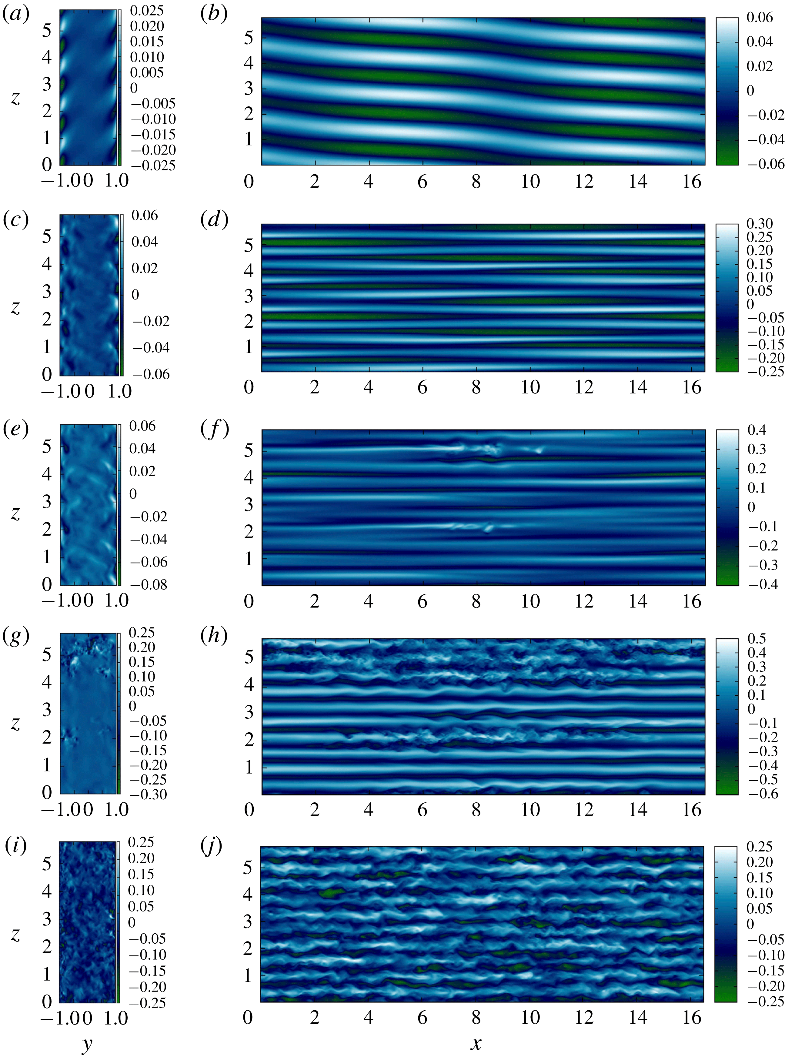
Figure 11. Snapshots of $w$
in
$w$
in $(y,z)$
planes (left) and
$(y,z)$
planes (left) and $u$
in
$u$
in $(x,z)$
planes (right) at various times for the linearly unstable
$(x,z)$
planes (right) at various times for the linearly unstable $Re=10\,000$
,
$Re=10\,000$
, $F_{h}^{-2}=0.2$
flow geometry: (a) early time
$F_{h}^{-2}=0.2$
flow geometry: (a) early time $t=337$
shows the signal of linear normal modes; (b) intermediate time
$t=337$
shows the signal of linear normal modes; (b) intermediate time $t=725$
shows nonlinear internal waves; (c) intermediate time
$t=725$
shows nonlinear internal waves; (c) intermediate time $t=1048$
shows the growth of wave-induced shear and smaller vertical wavelengths; (d) intermediate time
$t=1048$
shows the growth of wave-induced shear and smaller vertical wavelengths; (d) intermediate time $t=1070$
shows the ensuing Kelvin–Helmholtz-type overturning; (e) late time
$t=1070$
shows the ensuing Kelvin–Helmholtz-type overturning; (e) late time $t=1335$
shows the eventual and sustained growth of streaky flow indicative of the SSP/VWI attractor. See also accompanying movie (Movie 2.gif) in the supplementary material.
$t=1335$
shows the eventual and sustained growth of streaky flow indicative of the SSP/VWI attractor. See also accompanying movie (Movie 2.gif) in the supplementary material.
There are also episodes of more turbulent behaviour where the dissipation rate and mixing efficiency increase and smaller scales are observed in the flow fields. The times of maxima in the turbulent kinetic energy, dissipation and mixing are coincident with local accelerations of the flow and shear-induced overturns associated with instability of the internal waves (see the bottom two panels of figure 10), due presumably to either wave–wave or wave–mean flow resonance (see Grimshaw Reference Grimshaw1977; McComas & Bretherton Reference McComas and Bretherton1977; Sutherland Reference Sutherland2001), and will be a topic of future research. There is also some suggestion of a characteristic recurrence time scale for the bursting events in the energetics shown in figure 9, drawing some similarity to the bursts described in LCK (see in particular § A.1), which we may expect to recur if the simulation were continued.
At $Re=10\,000$
,
$Re=10\,000$
, $F_{h}^{-2}=0.2$
it is actually possible to choose a geometry which supports the (supercritical) linear instability while still remaining below the boundary for SSP/VWI turbulence. This particular flow geometry allows us to consider the competition between the nonlinear dynamics and different possible routes to turbulence. We perform another DNS at this
$F_{h}^{-2}=0.2$
it is actually possible to choose a geometry which supports the (supercritical) linear instability while still remaining below the boundary for SSP/VWI turbulence. This particular flow geometry allows us to consider the competition between the nonlinear dynamics and different possible routes to turbulence. We perform another DNS at this $Re$
and
$Re$
and $F_{h}$
with
$F_{h}$
with $L_{x}=16.5$
and
$L_{x}=16.5$
and $L_{z}=5.8$
(now with
$L_{z}=5.8$
(now with $N_{x}=N_{z}=512$
) and initialised with a large-scale yet small-amplitude initial condition. In this geometry we also expect the fastest growing linear mode to have one wavelength in the
$N_{x}=N_{z}=512$
) and initialised with a large-scale yet small-amplitude initial condition. In this geometry we also expect the fastest growing linear mode to have one wavelength in the $x$
-direction and four wavelengths in the
$x$
-direction and four wavelengths in the $z$
-direction. In this case we see again the initial exponential growth of the linear normal mode, saturating with the nonlinear internal wave dynamics, and spending a significant time there (as shown in the top two panels of figure 11).
$z$
-direction. In this case we see again the initial exponential growth of the linear normal mode, saturating with the nonlinear internal wave dynamics, and spending a significant time there (as shown in the top two panels of figure 11).
However, this is not the long-time attractor. Significantly, the finite amplitudes reached are sufficient to seed the SSP/VWI sustained turbulence which was observed in the linearly stable geometry. In other words, apparently, the linear instability simply provides another route to what appears to be the same attractor at these parameter values. This is borne out by the flow fields in figure 11 and the energetics of figure 9 (see also accompanying movie (Movie 2.gif) in the supplementary material). We find that when the local accelerations are energetic enough to give rise to overturns (as in the flow with $F_{h}^{-2}=0.7$
) the transfer of energy to small scales initiates the near-wall regeneration mechanism and sustained SSP/VWI turbulence is established as the late time attractor (see bottom 3 panels of figure 11). The energetics in figure 9 also approach the values associated with the linearly stable flow, which has undergone subcritical transition at late times, though there is undoubtedly a very significant (and long-lived) transient adjustment. It is worth noting that the flow fields after overturning in the
$F_{h}^{-2}=0.7$
) the transfer of energy to small scales initiates the near-wall regeneration mechanism and sustained SSP/VWI turbulence is established as the late time attractor (see bottom 3 panels of figure 11). The energetics in figure 9 also approach the values associated with the linearly stable flow, which has undergone subcritical transition at late times, though there is undoubtedly a very significant (and long-lived) transient adjustment. It is worth noting that the flow fields after overturning in the $F_{h}^{-2}=0.7$
case appear to show some transient growth towards an SSP/VWI configuration before stratification suppresses the spanwise streak scale, the small scales decay viscously and the internal wave regime recurs. This can be partially observed in the final panel of figure 10 and in the r.m.s., energetics and mixing efficiency reaching similar levels as observed in the wall-localised turbulence case in figure 9. Extrapolating then towards the relaminarisation boundary we expect such transient growth to increase until the boundary is crossed and the streaky flow becomes sustained.
$F_{h}^{-2}=0.7$
case appear to show some transient growth towards an SSP/VWI configuration before stratification suppresses the spanwise streak scale, the small scales decay viscously and the internal wave regime recurs. This can be partially observed in the final panel of figure 10 and in the r.m.s., energetics and mixing efficiency reaching similar levels as observed in the wall-localised turbulence case in figure 9. Extrapolating then towards the relaminarisation boundary we expect such transient growth to increase until the boundary is crossed and the streaky flow becomes sustained.
We conclude that below the relaminarisation criterion described in § 3.1 the turbulent attractor looks unaffected by the new linear instability, although it is undoubtedly important that a new linear instability mechanism has been identified to provide a route for small perturbations to excite turbulence.
5 Discussion and conclusions
The computations performed here have revealed another example of coherent layering of an initially linear density distribution at moderate stratification. This has more than a passing resemblance to the exact coherent structures isolated in LCK: shear-wise flow advects the streamwise velocity component to create an alternating, or zig-zagging structure. Confinement by the walls results in the shear-wise flow being associated with a streamwise vortex, whereas in the periodic geometry the shear-wise flow is periodic in $y$
. This is analogous to the rotation/advection of the vortex dipole necessary for the zig-zag instability (Billant & Chomaz Reference Billant and Chomaz2000b
). Importantly however, in the wall-bounded case the basic flow profile remains linearly stable in the parameter regimes studied here, meaning that the layering structures have a different generating mechanism. (In theory it may be possible to perform a homotopy of an exact coherent structure from a system with a stress-free boundary condition and horizontally shearing base flow which experiences a zig-zag-type linear instability and thus connect to the no-slip boundary condition considered here.)
$y$
. This is analogous to the rotation/advection of the vortex dipole necessary for the zig-zag instability (Billant & Chomaz Reference Billant and Chomaz2000b
). Importantly however, in the wall-bounded case the basic flow profile remains linearly stable in the parameter regimes studied here, meaning that the layering structures have a different generating mechanism. (In theory it may be possible to perform a homotopy of an exact coherent structure from a system with a stress-free boundary condition and horizontally shearing base flow which experiences a zig-zag-type linear instability and thus connect to the no-slip boundary condition considered here.)
The results here bear some similarity to the buoyancy patterns described in Leclercq et al. (Reference Leclercq, Partridge, Augier, Caulfield, Dalziel and Linden2016b ) for the axially stratified Taylor–Couette flow case, in so far as having sharper gradients confined near the walls and offset across the gap. We have also associated these density perturbations with a large-scale vortical flow, however it seems that the underlying mechanisms producing these structures are different again. Here we find the large-scale flow to be the modification of an existing secondary flow in plane Couette flow, whereas the suggestion in Leclercq et al. (Reference Leclercq, Partridge, Augier, Caulfield, Dalziel and Linden2016b ) is of a different nonlinear mechanism incorporating spiral modes, associated with various linear instabilities of the underlying flow, as also discussed in Park et al. (Reference Park, Billant and Baik2017) and Park et al. (Reference Park, Billant, Baik and Seo2018). How these two mechanisms connect as the narrow-gap limit is approached is therefore an interesting open question.
The other main finding of this work is the extent to which the laminar–turbulent boundary becomes affected by stratification in this flow geometry and in particular how the mechanism responsible for shutting off turbulence as stratification is increased has a fundamentally different interpretation from the flow with vertical shear/wall-normal stratification. Here, the intersection of a buoyancy-dominated large scale and the smaller inner scale of the near-wall regeneration mechanism is the key process by which relaminarisation occurs. This is in contrast to the vertical shearing case where the length scale associated with the flux of momentum into the interior is modified by stratification, as quantified by the magnitude of the Monin–Obukhov length in wall units (see Flores & Riley (Reference Flores and Riley2010) and Deusebio et al. (Reference Deusebio, Caulfield and Taylor2015) for more details) and found to predict relaminarisation. One may also make the observation that in the vertically shearing case buoyancy directly penalises the wall-normal flow responsible for lifting up the wall fluid to form the streaks. On the other hand, in the horizontally shearing orientation this wall-normal flow is indirectly penalised via its coupling with spanwise velocity in the streamwise rolls. Both cases limit the rolls, however the subtle, but crucial, difference regarding the velocity components is the reason for higher buoyancy forces (i.e. $F_{h}^{-2}$
or
$F_{h}^{-2}$
or $Ri$
) at large Reynolds number allowing sustained turbulence in the spanwise stratified orientation.
$Ri$
) at large Reynolds number allowing sustained turbulence in the spanwise stratified orientation.
Two important features of subcritical transition which we have not investigated thoroughly are computational domain size and initial conditions. We conjecture that our relaminarisation boundary may also be considered an ‘intermittency boundary’ and that there will only be some weak dependence of the turbulent fraction with $F_{h}$
at a given
$F_{h}$
at a given $Re$
(similar to figure 18 in Deusebio et al.
Reference Deusebio, Caulfield and Taylor2015). Recall, the mechanism is ultimately the suppression of streamwise rolls by buoyancy. This can be considered a local, high Reynolds number process, independent of viscosity. We may then conjecture that this relaminarisation mechanism is (largely) independent of box size and therefore we may only expect intermittency when
$Re$
(similar to figure 18 in Deusebio et al.
Reference Deusebio, Caulfield and Taylor2015). Recall, the mechanism is ultimately the suppression of streamwise rolls by buoyancy. This can be considered a local, high Reynolds number process, independent of viscosity. We may then conjecture that this relaminarisation mechanism is (largely) independent of box size and therefore we may only expect intermittency when $l_{z}\approx l_{S}$
. Likewise we expect the effect of initial conditions to be modest. We have shown how the turbulent attractor is disrupted by stratification and have not concerned ourselves with the particular pathways to that attractor. A more thorough investigation of these aspects is left for future research.
$l_{z}\approx l_{S}$
. Likewise we expect the effect of initial conditions to be modest. We have shown how the turbulent attractor is disrupted by stratification and have not concerned ourselves with the particular pathways to that attractor. A more thorough investigation of these aspects is left for future research.
The results presented here open a number of further research questions and opportunities. It would be of interest if these inherently nonlinear (i.e. not obviously and directly connected to a linear formation mechanism) and turbulent layers are observable in a laboratory experiment similar to those conducted by Facchini et al. (Reference Facchini, Favier, Le Gal, Wang and Le Bars2018). We note here that all of the physical and numerical experiments conducted by Facchini et al. (Reference Facchini, Favier, Le Gal, Wang and Le Bars2018), with the exception of cases where $F_{h}=\infty$
, are well above the relaminarisation boundary for subcritical turbulence that we have established. This may open a new avenue for connecting laboratory and numerical experiments involving layers and pattern formation in stratified turbulence. Robustness of these layers to changes in Prandtl number is therefore an obvious consideration; using salt as a stratifying agent increases the Prandtl number, or more precisely the Schmidt number, to
$F_{h}=\infty$
, are well above the relaminarisation boundary for subcritical turbulence that we have established. This may open a new avenue for connecting laboratory and numerical experiments involving layers and pattern formation in stratified turbulence. Robustness of these layers to changes in Prandtl number is therefore an obvious consideration; using salt as a stratifying agent increases the Prandtl number, or more precisely the Schmidt number, to ${\approx}700$
. It is at least plausible that even sharper gradients of density might arise in flows at larger
${\approx}700$
. It is at least plausible that even sharper gradients of density might arise in flows at larger $Pr$
, and it is also conceivable that these layers might penetrate further into the interior.
$Pr$
, and it is also conceivable that these layers might penetrate further into the interior.
Furthermore, the boundary conditions on $\unicode[STIX]{x1D70C}$
are chosen to satisfy a no-flux condition. However, if heat were used as the stratifying agent then it might be expected that there would be some heat loss through the side walls. A test case (results not shown) suggests that applying an insulating boundary condition, i.e. setting
$\unicode[STIX]{x1D70C}$
are chosen to satisfy a no-flux condition. However, if heat were used as the stratifying agent then it might be expected that there would be some heat loss through the side walls. A test case (results not shown) suggests that applying an insulating boundary condition, i.e. setting $\unicode[STIX]{x1D70C}|_{y=-L_{y}}=\unicode[STIX]{x1D70C}|_{y=L_{y}}=0$
yields very similar near-wall layers and large-scale mean flows, suggesting a certain robustness of the bulk flow features reported here.
$\unicode[STIX]{x1D70C}|_{y=-L_{y}}=\unicode[STIX]{x1D70C}|_{y=L_{y}}=0$
yields very similar near-wall layers and large-scale mean flows, suggesting a certain robustness of the bulk flow features reported here.
Our results also highlight an interesting question concerning the role of the orientation of shear in more general environmental and industrial flows. For example, in pipes and ducts the mean flow will generically have shear at some non-trivial angle to the orientation of gravity. As noted previously, horizontal shear, particularly at sufficiently high $Re$
, is a more effective route to transfer energy from the mean flow to the turbulence (Jacobitz & Sarkar Reference Jacobitz and Sarkar1998) than purely vertical shear, and as we have shown the turbulence suppression mechanisms are quite different for each case. The question then arises as to how these mechanisms compete, and also how turbulence is deformed by stratification in more generic situations. Just to mention one example, it has recently been observed that horizontal confinement in a duct, and hence the inevitable introduction of spanwise shear to the Holmboe instability of a principally vertically sheared (relatively ‘sharp’) density interface gives rise to a new robust long-lived nonlinear coherent structure in the form of a ‘confined Holmboe wave’ (Lefauve et al.
Reference Lefauve, Partridge, Zhou, Dalziel, Caulfield and Linden2018). It remains to be seen how similar confinement might affect turbulent flows, even without the sharp density interface typically required for the initial occurrence of Holmboe-type instabilities.
$Re$
, is a more effective route to transfer energy from the mean flow to the turbulence (Jacobitz & Sarkar Reference Jacobitz and Sarkar1998) than purely vertical shear, and as we have shown the turbulence suppression mechanisms are quite different for each case. The question then arises as to how these mechanisms compete, and also how turbulence is deformed by stratification in more generic situations. Just to mention one example, it has recently been observed that horizontal confinement in a duct, and hence the inevitable introduction of spanwise shear to the Holmboe instability of a principally vertically sheared (relatively ‘sharp’) density interface gives rise to a new robust long-lived nonlinear coherent structure in the form of a ‘confined Holmboe wave’ (Lefauve et al.
Reference Lefauve, Partridge, Zhou, Dalziel, Caulfield and Linden2018). It remains to be seen how similar confinement might affect turbulent flows, even without the sharp density interface typically required for the initial occurrence of Holmboe-type instabilities.
Finally, Taylor et al. (Reference Taylor, Deusebio, Caulfield and Kerswell2016) have shown how stratification can be a useful tool for studying the localisation and control of turbulence in vertically sheared flows. It is widely understood that large scale flows play some role in pattern formation and the transient growth and/or decay of localised turbulence (Duguet & Schlatter Reference Duguet and Schlatter2013; Lemoult, Aider & Wesfreid Reference Lemoult, Aider and Wesfreid2013; Couliou & Monchaux Reference Couliou and Monchaux2015). Here we have demonstrated how relaminarisation can be controlled by the buoyancy scale. It is therefore clearly of interest to investigate how the modification of large-scale flows discovered here influences the spatio-temporal behaviour of localised turbulence, and to what extent the control method of Taylor et al. (Reference Taylor, Deusebio, Caulfield and Kerswell2016) can be utilised to facilitate such an investigation. We intend to report the results of just such an investigation in due course.
Acknowledgements
We extend our thanks, for many helpful and enlightening discussions, to P. Linden, J. Taylor, S. Dalziel and the rest of the ‘MUST’ team in Cambridge and Bristol. We also offer a particular thanks to Q. Zhou for supplying us with the Monin–Obukhov generated intermittency boundary curve for the wall-normal stratified case. The source code, including linear stability code, is provided at https://bitbucket.org/dan_lucas/ spanwise-stratified-diablo and accompanying data can be found at https://doi.org/ 10.17863/CAM.37838. This work is supported by EPSRC Programme Grant EP/K034529/1 entitled ‘Mathematical Underpinnings of Stratified Turbulence’. The research presented here was initiated when D.L. was a postdoctoral researcher in DAMTP as part of the MUST programme grant.
Supplementary movies
Supplementary movies are available at https://doi.org/10.1017/jfm.2019.192.


