2.1. Dataset description

The dataset employed for the present study of wake dynamics is from the high-resolution LES of flow past a circular disk at Reynolds number $Re = U_\infty D/\nu = 5 \times 10^4$, reported in Chongsiripinyo & Sarkar (Reference Chongsiripinyo and Sarkar2020). Here, $U_\infty$ is the freestream velocity, $D$ is the disk diameter, and $\nu$ is the kinematic viscosity. The case of a homogeneous fluid from Chongsiripinyo & Sarkar (Reference Chongsiripinyo and Sarkar2020), who also simulate stratified wakes, is selected here. The filtered Navier–Stokes equations, subject to the condition of solenoidal velocity, were solved numerically on a structured cylindrical grid that spans a radial distance $r/D = 15$ and a streamwise distance $x/D = 125$. An immersed boundary method (Balaras Reference Balaras2004) is used to represent the circular disk in the simulation domain, and the dynamic Smagorinsky model (Germano et al. Reference Germano, Piomelli, Moin and Cabot1991) is used for the LES model. The numbers of grid points in the radial ($r$), azimuthal ($\theta$) and streamwise ($x$) directions are $N_r = 365$, $N_\theta = 256$ and $N_x = 4096$, respectively. The simulation has high resolution, with streamwise grid resolution $\Delta x = 10\eta$ at $x/D = 10$, where $\eta$ is the Kolmogorov length scale. By $x/D = 125$, the resolution improves to $\Delta x < 6\eta$ so that the onus on the subgrid model decreases progressively. Readers are referred to Chongsiripinyo & Sarkar (Reference Chongsiripinyo and Sarkar2020) for a detailed description of the numerical methodology and grid quality.

2.2. Spectral proper orthogonal decomposition

The SPOD technique is the frequency-domain variant of POD. It computes monochromatic modes that are optimal in terms of the energy norm of the flow, e.g. TKE for the wake flow at hand. The SPOD modes are the eigenvectors of the cross-spectral density matrix, which is estimated using Welch's approach (Welch Reference Welch1967). Here, we provide a brief overview of the method. For a detailed mathematical derivation and algorithmic implementation, readers are referred to Towne et al. (Reference Towne, Schmidt and Colonius2018) and Schmidt & Colonius (Reference Schmidt and Colonius2020).

For a statistically stationary flow, let $\boldsymbol {q}_i =\boldsymbol {q}(t_i)$ denote the mean subtracted snapshots, where $i =1,2,\ldots, n_t$ gives the number of snapshots. For spectral estimation, the dataset is first segmented into $n_{blk}$ overlapping blocks, with $n_{fft}$ snapshots in each block. The neighbouring blocks overlap by $n_{ovlp}$ snapshots, with $n_{ovlp}=n_{fft}/2$. The $n_{blk}$ blocks are then Fourier transformed in time, and all Fourier realizations of the $l$th frequency $\boldsymbol {q}^{(\,j)}_l$ are arranged in a matrix:

(2.1)\begin{equation} \hat{\boldsymbol{Q}}_{l}=\Big[\hat{\boldsymbol{q}}_{l}^{(1)}, \hat{\boldsymbol{q}}_{l}^{(2)}, \ldots, \hat{\boldsymbol{q}}_{l}^{(n_{blk})}\Big]. \end{equation}

The SPOD eigenvalues $\boldsymbol {\varLambda }_{l}$ are obtained by solving the eigenvalue problem

(2.2)\begin{equation} \frac{1}{n_{blk}}\,\hat{\boldsymbol{Q}}_{l}^{*}\boldsymbol{W} \hat{\boldsymbol{Q}}_{l} \boldsymbol{\varPsi}_{l}=\boldsymbol{\varPsi}_{l} \boldsymbol{\varLambda}_{l}, \end{equation}

where $\boldsymbol {W}$ is a positive-definite Hermitian matrix that accounts for the component-wise and numerical quadrature weights, and $(\cdot )^*$ denotes the complex conjugate. The SPOD modes at the $l$th frequency are recovered as

(2.3)\begin{equation} \boldsymbol{\varPhi}_{l} = \frac{1}{\sqrt{n_{blk}}}\,\hat{\boldsymbol{Q}}_{l} \boldsymbol{\varPsi}_{l} \boldsymbol{\varLambda}_{l}^{-1/2}. \end{equation}

The SPOD eigenvalues are denoted by $\boldsymbol {\varLambda }_{l}=\text {diag} \Big( \lambda _{l}^{(1)}, \lambda _{l}^{(2)}, \ldots, \lambda _{l}^{(n_{blk})} \Big)$. By construction, $\lambda _{l}^{(1)} \geq \lambda _{l}^{(2)} \geq \cdots \geq \lambda _{l}^{(n_{blk})}$ represent the energies of the corresponding SPOD modes that are given by the column vectors of the matrix $\boldsymbol {\varPhi }_{l}=\Big[\boldsymbol {\phi }_{l}^{(1)}, \boldsymbol {\phi }_{l}^{(2)}, \ldots, \boldsymbol {\phi }_{l}^{(n_{blk})} \Big]$. The SPOD mode $\boldsymbol {\phi }_{l}^{(\,j)}$ represents the $j$th dominant coherent flow structure at the $l$th frequency. An useful property of the SPOD modes is their orthogonality; the weighted inner product at each frequency is $\langle \boldsymbol {\phi }_{l}^{(i)},\boldsymbol {\phi }_{l}^{(\,j)}\rangle =(\boldsymbol {\phi }_{l}^{(i)})^*\boldsymbol {W} \boldsymbol {\phi }_{l}^{(\,j)}= \delta _{ij}$.

Here, we perform SPOD on various two-dimensional streamwise planes ranging from $x/D = 1$ to $x/D = 120$. Thus $\boldsymbol {q}$ contains the three velocity components at the discretized grid nodes on a streamwise-constant plane. These planes are sampled at spacing $5D$ from $x/D = 5$ to $x/D = 100$, and five additional planes are sampled at $x/D=1, 2, 3, 110, 120$. The utilized time series has $n_t = 7200$ snapshots, with uniform separation of non-dimensional time $\Delta t U_{\infty }/D = 0.072$ between two snapshots. Owing to the periodicity in the azimuthal direction, the flow field is first decomposed into azimuthal wavenumbers $m$,

(2.4)\begin{equation} q(x,r,\theta,t) = \sum_{m} \hat{q}_m(x,r,t), \end{equation}

and then SPOD is applied on the data at each azimuthal wavenumber. The spectral estimation parameters used here are $n_{fft}=512$ and $n_{ovlp}=256$, resulting in $n_{blk} = 27$ SPOD modes for each $St$. Each block used for the temporal fast Fourier transform spans a time duration $\Delta T = 36.91 U_\infty /D$.

2.3. Reconstruction using convolution approach

The convolution strategy proposed by Nekkanti & Schmidt (Reference Nekkanti and Schmidt2021) is employed for low-dimensional reconstruction of the flow field. This involves computing the expansion coefficients by convolving the SPOD modes over the data one snapshot at a time:

(2.5)\begin{equation} \boldsymbol{a}_l^{(i)}(t) = \int_{\Delta T} \int_{\varOmega} ( \boldsymbol{\phi}_l^{(i)}(x))^{*}\,\boldsymbol{W}(x)\,\boldsymbol{q}(x,t+\tau)\,w(\tau) \,{\rm e}^{-{\rm i} 2{\rm \pi} f_l\tau}\,\mathrm{d}\kern 0.06em x \,\mathrm{d} \tau. \end{equation}

Here, $w(\tau )$ is the Hamming windowing function, and $\varOmega$ is the spatial domain of interest. The data at time $t$ are then reconstructed as

(2.6)\begin{equation} \boldsymbol{q}(t) \approx \sum_{l}\sum_{i} a^{(i)}_l (t)\,\boldsymbol{\phi}^{(i)}_{l} \,{\rm e}^{-{\rm i} 2{\rm \pi} f_l t}. \end{equation}

2.4. Bispectral mode decomposition

Bispectral mode decomposition (BMD) is a technique proposed recently by Schmidt (Reference Schmidt2020) to characterize the coherent structures associated with triadic interactions in statistically stationary flows. Here, we provide a brief overview of the method. The reader is referred to Schmidt (Reference Schmidt2020) for further details of the derivation and mathematical properties of the method.

The BMD technique is an extension of classical bispectral analysis to multidimensional data. The classical bispectrum is defined as the double Fourier transform of the third moment of a time signal. For a time series $y(t)$ with zero mean, the bispectrum is

(2.7)\begin{equation} S_{yyy}(\,f_1,f_2)=\iint R_{yyy}(\tau_1,\tau_2) \,{\rm e}^{-{\rm i} 2{\rm \pi} (\,f_1 \tau_1 +f_2 \tau_2) }\,{\rm d}\tau_1 \,{\rm d}\tau_2, \end{equation}

where $R_{yyy}(\tau _1,\tau _2)=E[y(t)\,y(t-\tau _1)\,y(t-\tau _2)]$ is the third moment of $y(t)$, and $E[\cdot ]$ is the expectation operator. The bispectrum is a signal processing tool for one-dimensional time series that measures the quadratic phase coupling only at a single spatial point. In contrast, BMD identifies the intensity of the triadic interactions over the spatial domain of interest, and extracts the corresponding spatially coherent structures.

Also, BMD maximizes the spatial integral of the pointwise bispectrum:

(2.8)\begin{equation} b(\,f_k,f_l) = E\left[\int_\varOmega \hat{\boldsymbol{q}}^{*}(x,f_k) \circ \hat{\boldsymbol{q}}^{*}(x,f_l) \circ \hat{\boldsymbol{q}}(x,f_k+f_l)\,{\rm d} x\right]. \end{equation}

Here, $\hat {\boldsymbol {q}}$ is the temporal Fourier transform of $\boldsymbol {q}$ computed using the Welch (Reference Welch1967) approach, and $\circ$ denotes the Hadamard (or elementwise) product.

Next, as in (2.1), all the Fourier realizations at the $l$th frequency are arranged into the matrix $\hat {\boldsymbol {Q}}_{l}$. The auto-bispectral matrix is then computed as

(2.9)\begin{equation} \boldsymbol{B} = \frac{1}{n_{blk}}\,\hat{\boldsymbol{Q}}_{k\circ l}^{H}\boldsymbol{W}\hat{\boldsymbol{Q}}_{k+l} , \end{equation}

where $\hat {\boldsymbol {Q}}_{k\circ l}^{H} = \hat {\boldsymbol {Q}}_{k}^{*}\circ \hat {\boldsymbol {Q}}_{l}^{*}$.

To measure the interactions between different quantities, we construct the cross-bispectral matrix

(2.10)\begin{equation} \boldsymbol{B}_c = \frac{1}{n_{blk}}\,(\hat{\boldsymbol{Q}}_{k}^{*}\circ\hat{\boldsymbol{R}}_{l}^{*}) \boldsymbol{W}\hat{\boldsymbol{S}}_{k+l}. \end{equation}

In the present application, matrices $\boldsymbol {Q}$, $\boldsymbol {R}$ and $\boldsymbol {S}$ comprise the time series of the field variables at the azimuthal wavenumber triad [$m_1, m_2, m_3]$.

Owing to the non-Hermitian nature of the bispectral matrix, the optimal expansion coefficients $\boldsymbol {a}_1$ are obtained by maximizing the absolute value of the Rayleigh quotient of $\boldsymbol {B}$ (or $\boldsymbol {B}_c$):

(2.11)\begin{equation} \boldsymbol{a}_1 = \arg\max_{\|\boldsymbol{a}\|=1} \left|\frac{\boldsymbol{a}^*\boldsymbol{B}\boldsymbol{a}}{\boldsymbol{a}^*\boldsymbol{a}}\right|. \end{equation}

The complex mode bispectrum is then obtained as

(2.12)\begin{equation} \lambda_1(\,f_k,f_l) = \left|\frac{\boldsymbol{a}_1^*\boldsymbol{B}\boldsymbol{a}_1} {\boldsymbol{a}_1^*\boldsymbol{a}_1}\right|. \end{equation}

Finally, the leading-order bispectral modes and the cross-frequency fields are recovered as

(2.13)\begin{equation} \boldsymbol{\phi}_{k+l}^{(1)} = \hat{\boldsymbol{Q}}_{k+l}\boldsymbol{a}_{1} \end{equation}

and

(2.14)\begin{equation} \boldsymbol{\phi}_{k\circ l}^{(1)} = \hat{\boldsymbol{Q}}_{k\circ l}\boldsymbol{a}_{1}, \end{equation}

respectively. By construction, the bispectral modes and cross-frequency fields have the same set of expansion coefficients. This ensures explicitly the causal relation between the resonant frequency triad ($f_k, f_l, f_k+f_l)$, where $\hat {\boldsymbol {Q}}_{k\circ l}$ is the cause, and $\hat {\boldsymbol {Q}}_{k+l}$ is the effect. The complex mode bispectrum $\lambda _1$ measures the intensity of the triadic interaction, and the bispectral mode $\boldsymbol { \phi }_{k+l}$ represents the structures that result from the nonlinear triadic interaction.

Similar to SPOD, we perform BMD on various two-dimensional streamwise planes and use the same spectral estimation parameters $n_{fft}=512$ and $n_{ovlp}=256$. Since our focus is on interactions of different azimuthal wavenumbers, the cross-BMD method, which computes the cross-bispectral matrix $\boldsymbol {B}_c$, is applied to the wake database. The specific interactions among different $m$ and their analysis using BMD will be presented and discussed in § 5.1.

3.1. Streaky structures in the near and far wake

Nidhan et al. (Reference Nidhan, Chongsiripinyo, Schmidt and Sarkar2020) showed that the near and far fields of the wake of a circular disk are dominated by two distinct modes, residing at (i) $m=1$, $St = 0.135$, and (ii) $m=2$, $St \rightarrow 0$. While the former mode is the VS mode in the wake of a circular disk (Fuchs, Mercker & Michel Reference Fuchs, Mercker and Michel1979a; Berger et al. Reference Berger, Scholz and Schumm1990; Cannon et al. Reference Cannon, Champagne and Glezer1993), the physical origin of the latter mode remains unclear. Johansson & George (Reference Johansson and George2006) hint that the $m=2$ mode is linked to ‘very’ large-scale features that twist the mean flow slowly. Motivated by the findings of Nidhan et al. (Reference Nidhan, Chongsiripinyo, Schmidt and Sarkar2020) and the discussion in Johansson & George (Reference Johansson and George2006), we investigate the streamwise manifestation of the azimuthal modes $m=1$ and $m=2$. The main result is that, different from the $m =1$ mode, the $m =2$ mode is associated with streamwise-aligned streaky structures.

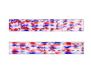
Figure 1 shows the azimuthal modes $m=1$ and $m=2$ of an instantaneous flow snapshot in the wake spanning downstream distance $0 < x/D < 100$, obtained using a Fourier transform in the azimuthal direction $\theta$. In the $m=1$ mode (figure 1a), a wavelength $\lambda /D = 1/St_{VS}$ (where the VS frequency is $St_{VS} \approx 0.13\unicode{x2013}0.14$) is evident throughout the domain. This observation is in agreement with previous studies (Johansson et al. Reference Johansson, George and Woodward2002; Johansson & George Reference Johansson and George2006; Nidhan et al. Reference Nidhan, Chongsiripinyo, Schmidt and Sarkar2020) that report the existence of the VS mode at significantly large downstream locations ${\sim } O(100D)$ from the disk.

Figure 1. Azimuthally decomposed instantaneous fields of the streamwise velocity ($u_x$) for (a) $m = 1$ and (b) $m = 2$ azimuthal modes. Rectangular boxes in (b) show large-scale streaks in the $m=2$ field.

The spatial structure of the $m=2$ mode (figure 1$b$) is quite different from that of the $m=1$ mode. In the $m=2$ mode visualization, distinct elongated structures are present throughout the domain. Notice in particular the structures inside the dashed rectangular boxes. The streamwise extent of these structures can be up to $\lambda _x/D \approx 25$ (see $70 < x/D < 95$), significantly larger than the wavelength of the VS mode $\lambda _x/D \approx 7$.

Figures 2(a,c) show the instantaneous streamwise velocity field in the near–intermediate and intermediate–far wakes, respectively, of the disk on a $x/D\unicode{x2013}\theta$ plane. The $x/D\unicode{x2013}\theta$ plane is constructed by unrolling the cylindrical surface at a constant $r/D$. For the near–intermediate field (figure 2a), the plane is located at $r/D = 1.25$, while for the intermediate–far field (figure 2c), $r/D = 2.5$ is chosen. In both figures, VS structures are evident, spaced at an approximate wavelength $\lambda _x/D \approx 7$. These structures and the wavelength $\lambda _x/D \approx 7$ become even more evident when the flow fields at the respective radial locations in the near–intermediate and intermediate–far wakes are constructed with only the $m=1$ mode, as shown in figures 2(b,d). Upon removing the contribution of the VS mode that lies in the $m=1$ azimuthal wavenumber (Johansson et al. Reference Johansson, George and Woodward2002; Johansson & George Reference Johansson and George2006; Nidhan et al. Reference Nidhan, Chongsiripinyo, Schmidt and Sarkar2020), the streaks become readily apparent in figures 2(b,d). See again the structures contained inside dashed rectangular boxes in figures 2(e,f). These observations in figures 1 and 2 are strong initial indications of the presence of large-scale streaks in turbulent wakes, similar to those reported recently in the numerical and experimental datasets of turbulent jets (Nogueira et al. Reference Nogueira, Cavalieri, Jordan and Jaunet2019; Pickering et al. Reference Pickering, Rigas, Nogueira, Cavalieri, Schmidt and Colonius2020). In what follows, the characteristics and robustness of these elongated structures are quantified through various statistical and spectral measures.

Figure 2. Instantaneous streamwise velocity on $x/D\unicode{x2013}\theta$ planes at (a,b,e) $r/D = 1.25$ and (c,d,f) $r/D = 2.5$. Plots (a,c) show the full streamwise velocity field; (b,d) show the field reconstructed from the $m=1$ contribution only; (e,f) show the field with the $m=1$ contribution removed. Rectangular boxes in (e,f) emphasize the large-scale streaks in the flow field with the $m=1$ mode removed.

To this end, we invoke Taylor's hypothesis, converting time $t$ at a location $x_0$ to pseudo-streamwise distance from $x_0$: $x_t = U_{conv} t$, where $U_{conv} = U_{\infty } - U_d$ is the convective velocity. Since the defect velocity in the wake is $U_d \ll U_\infty$ (where $U_\infty$ is the freestream velocity), $U_{conv}$ is approximated by $U_{\infty }$. Taylor's hypothesis requires velocity fluctuation to be sufficiently small compared to $U_{conv}$. Figure 3 shows that this requirement is met since turbulence intensity ($K^{1/2}/U_\infty$) drops below $12\,\%$ beyond $x/D = 10$ for all radial locations, and below $4\,\%$ at $x/D = 30$. Previous work on turbulent wakes has shown Taylor's hypothesis to be valid in the wake when $K^{1/2}/U_{\infty }$ drops below ${\sim } 10\,\%$ (Antonia & Mi Reference Antonia and Mi1998; Kang & Meneveau Reference Kang and Meneveau2002; Dairay, Obligado & Vassilicos Reference Dairay, Obligado and Vassilicos2015; Obligado, Dairay & Vassilicos Reference Obligado, Dairay and Vassilicos2016). Invoking Taylor's hypothesis gives $St \approx U_\infty k_x$. In this study, we will focus particularly on $St \rightarrow 0$ (obtained from either temporal spectra or SPOD at different $x/D$ locations), which, by Taylor's hypothesis, is equivalent to large-scale streaks with $k_x \rightarrow 0$ ($k_x$ being the streamwise wavenumber) at those locations.

Figure 3. Turbulence intensity ($K^{1/2}/U_{\infty }$) as a function of streamwise ($x$) and radial ($r$) directions. The magenta curve demarcates the region where $K^{1/2}/U_\infty$ reduces to 0.12.

The near-to-intermediate wake behaviour is shown at $x_0/D = 10$ in figures 4(a,c,e), and at $x_0/D = 20$ in figures 4(b,d,f), through plots of streamwise velocity fluctuation ($u'_x$) at $r/D = 0.8$ in the $x_t/D\unicode{x2013}\theta$ plane. Time $t$ is transformed to the $x_t$ coordinate by application of Taylor's hypothesis, which is valid beyond $x/D \ge 9$ in the wake, as was shown through figure 3 and the associated discussion.

Figure 4. Streamwise velocity fluctuations $u'_x$ on an $x_t/D$–$\theta$ plane at $r/D \approx 0.8$, for (a,c,e) $x_0/D = 10$, and (b,d,f) $x_0/D = 20$. Plots (a,b) include all azimuthal components; (c,d) exclude $m=1$; and (e,f) include solely $m=2$.

Due to the strong signature of the VS mode in the near-to-intermediate wake, alternate patches of inclined positive and negative fluctuations separated by 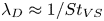$\lambda _D \approx 1/St_{VS}$ dominate the visualization in figures 4(a,b). It is known a priori that these structures are contained in the $m=1$ azimuthal mode. In order to assess space-time coherence other than the VS mode, the streamwise fluctuations are replotted in figures 4(c,d) after removing the $m=1$ contribution. Once the $m=1$ contribution is removed, streamwise streaks become evident at both locations. Furthermore, one can also observe that these streaks appear to be contained primarily in the azimuthal mode $m=2$, i.e. there are two structures over the azimuthal length of $2{\rm \pi}$. Only the $m=2$ component is shown in figures 4(e,f), where the elongated streamwise streaks come into sharper focus. Building upon figure 1, figures 4(c–f) lend support to the spatiotemporal robustness of these large-scale streaks in the turbulent wake of circular disk.

The downstream distance ($0< x/D<120$) spanned in the simulations of Chongsiripinyo & Sarkar (Reference Chongsiripinyo and Sarkar2020) is very large, thus enabling the far field to be probed too for the presence (or absence) of the streamwise streaks. Figures 5(a,c) show the $x_t/D\unicode{x2013}\theta$ plots of $u'_x$, with the contribution of the $m=1$ mode excluded, in regions starting at $x_0/D = 40$ and $80$. The $x_t/D\unicode{x2013}\theta$ planes are located at $r/D =2$ for these far-wake locations since the wake width grows with $x$. Interested readers can refer to figures 5, 15 and 16 of Chongsiripinyo & Sarkar (Reference Chongsiripinyo and Sarkar2020), and figure 5 of Nidhan et al. (Reference Nidhan, Chongsiripinyo, Schmidt and Sarkar2020), for an in-depth discussion about the mean and turbulence statistics. Similar to the near-wake plot in figures 4(c,d), large-scale streaks elongated in the streamwise direction are found to extend into the far wake as well. Once again, isolating the $m=2$ component (figures 5b,d) highlights the streaks. Collectively, figures 4 and 5 demonstrate that the streaks span the entire wake length and that the $m = 2$ mode drives these streaks.

Figure 5. The $u'_x$ field on a $x_t/D$–$\theta$ plane at $r/D \approx 2.0$, for (a,b) $x_0/D = 40$, and (c,d) $x_0/D = 80$. In (a,c), $m=1$ is removed, and in (b,d), only $m=2$ is shown.

Figure 6 shows two-dimensional spectra in the streamwise wavelength versus azimuthal mode ($k_x\unicode{x2013}m$) space at four representative streamwise locations, $x/D = 10$, 20, 40 and $80$. Here, $k_x$ is the wavenumber of the pseudo-streamwise direction $x_t$. The $m=1$ contribution is removed a priori to emphasize the large-scale streaks. At all these four locations, these streaky structures correspond to $k_x \rightarrow 0$ and are found to reside in the $m=2$ azimuthal mode. Note that $k_x = 0$, $St=0$ should be interpreted as $k_x$, $St \rightarrow 0$ as the length of the time series is not sufficient to resolve the large time scale of streaks. In Appendix A, we vary the spectral estimation parameter $n_{fft}$ to resolve the lower frequencies and identify the frequency associated with streaks in this limit to be $St \approx 0.006$.

Figure 6. Two-dimensional power spectral density of the streamwise velocity fluctuation in $k_x\unicode{x2013}m$ space, for: (a) $x/D = 10$, $r/D \approx 0.8$; (b) $x/D = 20$, $r/D \approx 0.8$; (c) $x/D = 40$, $r/D \approx 2.0$; (d) $x/D = 80$, $r/D \approx 2.0$. The $m=1$ wavenumber is removed so as to de-emphasize the VS structure.

3.2. Evidence of lift-up mechanism in the wake

Previous work in turbulent free shear flows and wall-bounded flows often attributes the formation of streaks in the velocity to the lift-up mechanism (Ellingsen & Palm Reference Ellingsen and Palm1975; Landahl Reference Landahl1975). The lift-up mechanism, by sweeping fluid from high-speed regions to low-speed regions, and vice versa, leads to the formation of high-speed and low-speed streaks, respectively. Brandt (Reference Brandt2014) provides a comprehensive review of the lift-up mechanism and its crucial role in various fundamental phenomena, e.g. subcritical transition in shear flows, self-sustaining cycle in wall bounded flows, and disturbance growth in complex flows.

To investigate the presence of the lift-up mechanism in the wake, we plot conditional averages of streamwise vorticity fluctuations ($\omega _x$) at three representative locations in the flow – the planes $x/D = 10$, 40 and $80$ in figure 7. Figures 7(a,b,c) show a conditional average $\langle \omega ^{c1}_x \rangle$ designed to extract the structure of the streamwise vorticity on a constant-$x$ plane during times of large streamwise velocity fluctuations. Specifically, the condition is that

(3.1)\begin{equation} u'_x \ge c(u'_x)^{rms} \end{equation}

at a specified point P on that plane, and $\langle \omega ^{c1}_x \rangle$ is the temporal average of all $\omega _x (t)$ that satisfy this condition. The conditional point P (shown as green dots in figure 7) is chosen to lie at $\theta = 0$ and radial locations $r/D = 0.8$ and $2$ for $x/D = 10$ and $x/D=40, 80$, respectively. The selection of different radial locations at $x/D = 10$ and $x/D=40, 80$ is based on the approximate values of mean wake half-widths at the respective $x/D$ locations (Chongsiripinyo & Sarkar Reference Chongsiripinyo and Sarkar2020). Owing to rotational invariance of statistics for an axisymmetric wake, the condition is applied to a new point ${\rm P}_1$ at the same $r/D$ but a different value of $\theta$, and the new $\langle \omega ^{c1}_x \rangle$ field, after a rotation to bring ${\rm P}_1$ to P, is included in the conditional average. Since $N_\theta = 256$ points are used for discretization, the ensemble used for the conditional average is expanded significantly by exploiting rotational invariance of statistics. Figures 7(d,e,f) show $\langle \omega ^{c2}_x \rangle$ computed using a different condition at point P,

(3.2)\begin{equation} -u'_xu'_r \ge c(-u'_xu'_r)^{rms} . \end{equation}

Figure 7. Conditionally-averaged streamwise vorticity at (a,d) $x/D = 10$, (b,e) $x/D = 40$, and (c,f) $x/D = 80$. Plots (a,b,c) show $\langle \omega ^{c1}_x \rangle$, conditioned using $u'_x$, and (d,e,f) show $\langle \omega ^{c2}_x \rangle$, conditioned using $u'_xu'_r$. The green dot shows the location of the conditioning point: (a,d) $r/D \approx 0.8$, $\theta \approx 0^{\circ }$, and (b,c,e,f) $r/D \approx 2$, $\theta \approx 0^{\circ }$. The radial domain extends until $r/D = 2$ at $x/D =10$, and until $r/D = 5$ at $x/D=40, 80$. Positive vorticity (red) is out of the plane, and negative vorticity (blue) is into the plane.

This condition is designed to identify the structure of streamwise vorticity at times of significant Reynolds shear stress at point P. The results exhibit moderate sensitivity to $c \in (0, 1]$, as reported in Appendix B. Hence $c$ is set to $0.5$ as a compromise between identification of intense events and retention of sufficient snapshots for conditional averaging. Here, $(u'_x)^{rms}$ and $(-u'_x u'_r)^{rms}$ are the root-mean-square (r.m.s.) values of the streamwise velocity fluctuations and the r.m.s. values of the streamwise–radial fluctuations correlation at the conditioning points, respectively.

The conditionally averaged field based on (3.1) captures the structure of the streamwise vorticity field during events of intense positive $u'_x$. In figure 7(a), two rolls of streamwise vorticity are observed in the conditionally averaged field: negative on the top and positive at the bottom of the conditioning point, respectively. These streamwise vortex rolls push the high-speed fluid in the outer wake to the low-speed region in the inner wake around the conditioning points (green dot), leading to $u'_x> 0$. When the averaging procedure is conditioned on negative streamwise velocity fluctuations, i.e. $u'_x \leq -c(u'_x)^{rms}$, the signs of the vortex rolls in figure 7 are interchanged, as expected (not shown). At $x/D = 40$ and $80$ (figures 7b,c), two additional vortical structures are observed in the $\theta = [90^{\circ }, 270^{\circ }]$ region. However, around the conditioning point, the spatial organization of vorticity remains qualitatively similar. The size of these vortex rolls increases with $x/D$, consistent with the radial spread of the wake.

The conditionally averaged field based on (3.2) captures the vorticity field corresponding to intense positive $-u'_xu'_r$ values. In a turbulent wake, $-u'_xu'_r$ is predominantly positive such that the dominant production term in the wake, $P_{xr} = \langle -u'_xu'_r \rangle \,\partial U /\partial r > 0$, acts to transfer energy from the mean flow to turbulence. Now turning to (3.2), positive $-u'_xu'_r$ can result from two scenarios: (i) $u'_r > 0$, $u'_x < 0$, i.e. ‘ejection’ of low-speed fluid from the inner wake to the outer wake; and (ii) $u'_r < 0$, $u'_x > 0$, i.e. ‘sweep’ of high-speed fluid from outer wake to inner wake. Both of the above-mentioned scenarios are consistent with the lift-up mechanism. If ejection and sweep events were equally probable, then $\langle \omega ^{c2}_x \rangle \approx 0$ due to the opposite spatial distribution of vortices during ejection and sweep events. However, $\langle \omega _x^{c2}\rangle$ obtained from $-u'_xu'_r$ based conditioning (figures 7d,e,f) shows that the positive and negative vortices are spatially organized such that the flow induced by these vortices at the conditioning point is outwards ($u'_r > 0$), pushing low-speed fluid from the inner wake to the outer wake. In short, $\langle \omega ^{c2}_{x} \rangle$ fields in figures 7(d,e,f) correspond to the ejection events at the conditioning point. A similar spatial organization of $\langle \omega ^{c2}_x \rangle$ is observed across the wake cross-section when the radial location of the conditioning point is varied (plots not shown for brevity). This observation establishes that ejections are the dominant contributors to intense positive $-u'_xu'_r$, as opposed to sweep events, therefore ejections are more instrumental in the energy transfer from mean to turbulence. Previous studies (Kline et al. Reference Kline, Reynolds, Schraub and Runstadler1967; Corino & Brodkey Reference Corino and Brodkey1969; Wallace Reference Wallace2016) of the turbulent boundary layer have also reported that ejection events are the primary contributors to Reynolds shear stress.

Figure 7 has two important implications. First, figures 7(a,b,c) demonstrate strong correlation between intense $u'_x$ fluctuations and distinct streamwise vortical structures, indicating that the lift-up mechanism is active in the turbulent wake, in both the near field and the far field. Second, the conditionally averaged fields obtained using $u'_xu'_r$ inform us that the lift-up mechanism corresponding to the ejection of low-speed fluid from the inner wake to the outer wake is more dominant than the sweep of high-speed fluid from the outer wake to the inner wake. To the best of the authors’ knowledge, both these observations constitute the first numerical evidence in the near and far fields of a canonical bluff body turbulent wake of (i) the lift-up mechanism, and (ii) the dominance of ejection events.

4.1. Energetics of streaky structures using SPOD analysis

The SPOD analysis is performed at different streamwise locations ($x/D$) in $1 \le x/D \le 120$. By definition, the leading SPOD mode at a given $x/D$ represents the most energetic coherent structures at the associated frequency ($St$) and azimuthal wavenumber ($m$). Figure 8 shows the percentage of energy in the leading SPOD modes ($\lambda ^{(1)}$) as a function of frequency and streamwise distance for the first six azimuthal wavenumbers, $m = 0$ to $m=5$. The percentage of energy at each streamwise location is obtained by normalizing the leading eigenvalue with the total TKE, $E^{T}_k(x/D)$, at the corresponding location. Overall, the most significant contributors to the TKE are the VS mode ($m=1$, $St=0.135$) and the mode corresponding to streaks ($m=2$, $St \rightarrow 0$), as reported in Nidhan et al. (Reference Nidhan, Chongsiripinyo, Schmidt and Sarkar2020). The leading VS SPOD mode contains about 10 % energy in the near-wake region ($5 \lesssim x/D \lesssim 15$) and decreases thereafter. The leading SPOD mode corresponding to the streaks in the $m=2$ mode contains approximately 3 % energy from $x/D=10$ onwards. The axisymmetric component ($m=0$) exhibits a peak at $St \rightarrow 0.054$ at $x/D=1$, and a much smaller peak at $St \approx 0.19$ for $10 \lesssim x \lesssim 120$. The former is associated with the pumping of the recirculation bubble (Berger et al. Reference Berger, Scholz and Schumm1990), whereas the latter was observed in previous studies (see figure 12 in Berger et al. (Reference Berger, Scholz and Schumm1990), and figure 7 in Fuchs, Mercker & Michel (Reference Fuchs, Mercker and Michel1979b)) but was not investigated further. The $m = 0$ mode is not the focus of this study.

Figure 8. Percentage of energy contained in the leading SPOD modes $\lambda ^{(1)}$ as a function of frequency $St$ and streamwise location $x/D$ at different azimuthal wavenumbers: (a) $m = 0$, (b) $m = 1$, (c) $m = 2$, (d) $m = 3$, (e) $m = 4$, and (f) $m = 5$. The leading SPOD eigenvalue $\lambda ^{(1)}(St,x/D)$ is normalized with the total TKE $E_k^{T}(x/D)$ at the corresponding streamwise location, to calculate the percentage contribution.

The energy $\lambda ^{(1)}$ contained in the higher azimuthal wavenumbers ($m=3\unicode{x2013}5$) is shown in figures 8(d–f), respectively. Although $\lambda ^{(1)}$ is smaller than at $m=1$ or $m=2$, the higher modes also exhibit temporal structure. The $m=3$ component shows energy concentration at the VS frequency $St=0.135$ for $15 \lesssim x/D \lesssim 70$, and at $St \rightarrow 0$ for $x/D \gtrsim 50$. For $m=4$, energy is concentrated near $St \rightarrow 0$ for $x/D \gtrsim 60$. For the $m=5$ component, traces of the VS mode and streaks ($St \rightarrow 0$) are observed at the streamwise locations $x/D \gtrsim 60$ and $x/D \gtrsim 80$, respectively. Figure 8 indicates that the peaks at the VS frequency are present only at the odd azimuthal wavenumbers ($m=1,3,5$), whereas the peaks corresponding to the large-scale streaks, i.e. $St \rightarrow 0$, can be found at both odd and even $m$. It is also interesting to note that for higher $m$, both the VS modes and streaks do not appear until larger values of $x/D$. This suggests nonlinear interactions among different frequencies and azimuthal wavenumbers as the wake evolves, as will be elaborated in § 5.

The $St \rightarrow 0$ streaks are dominated by the $m =2$ azimuthal wavenumber, as demonstrated by figure 9(a), which shows the contribution of different $m$ at $St \rightarrow 0$. The leading eigenvalues of each azimuthal wavenumber are normalized by the total energy at $St \rightarrow 0$, i.e. $\sum _m \sum _i \lambda ^{(i)} (St\rightarrow 0,m)$. Streaks are azimuthally non-uniform structures and are not present in the axisymmetric $m=0$ component. Hence we focus on $m \ge 1$. The azimuthal wavenumber $m=2$ is energetically dominant at the $St \rightarrow 0$ frequency, containing about 40–50 % of the total energy at $St \rightarrow 0$. The suboptimal wavenumber is $m=3$ for $5\le x \le 80$, and switches between $m=3$ and $m=4$ thereafter. However, the difference in energy between the $m=2$ and $m=3$ wavenumbers is always large, >30 %. This dominance of the $m=2$ wavenumber at $St \rightarrow 0$ is also consistent with the visualizations of the streamwise velocity fluctuations in figures 4 and 5, where one can see the presence of $m=2$ even with the naked eye.

Figure 9. (a) Contributions of the leading SPOD modes $\lambda ^{(1)}$ at different azimuthal wavenumbers to $St \rightarrow 0$. (b) Percentage energy contained in the frequencies $St=0.135$ and $St\rightarrow 0$.

The energetic contribution of the two dominant frequencies, $St=0.135$ (VS) and $St \rightarrow 0$ (streaks), is compared by computing the percentage of total energy (across all $m$ and $i$) at a given frequency $St$ as

(4.1)\begin{equation} \xi(St;x/D)=\frac{\displaystyle\sum_m \sum_i \lambda^{(i)}(m,St;x/D)}{E^{T}_k(x/D)} \times 100. \end{equation}

Figure 9(b) shows that the VS frequency is more dominant in the region $x\le 70$, whereas the zeroth frequency dominates for $x\ge 70$. This implies that although the streaks are present throughout, they are energetically more prominent in the far-wake region. It is interesting to note that beyond $x/D \approx 65$, the defect velocity decay rate changes from $x^{-1}$ to $x^{-2/3}$ in the wake (Chongsiripinyo & Sarkar Reference Chongsiripinyo and Sarkar2020). For comparison, the most dominant component at the zeroth frequency, i.e. $m=2$, is also shown in figure 9(b), which exhibits a similar trend of increasing prominence in the downstream direction.

Having diagnosed the streaky structure ($m=2$, $St\rightarrow 0$) and the VS structure ($m=1$, $St=0.135$) using SPOD, we shift focus to their imprint on the flow in physical space by reconstructing the flow field using their leading five SPOD modes. The $m=2$ wavenumber is selected because it is energetically dominant at $St \rightarrow 0$. The reconstruction is performed using the convolution strategy described in § 2. Figures 10(a–c) show the instantaneous energy in the three fluctuation components $u'_x$, $u'_r$ and $u'_{\theta }$ at $x/D =10$, 40 and 80, after reconstruction with the streaky-structure SPOD modes. The instantaneous energy is depicted within the time interval $t \in [0, 110]$, which corresponds to the first five blocks used for SPOD, and is representative of the entire reconstructed flow fields. The energy of $u'_x$ is significantly higher than that of $u'_r$ and $u'_\theta$. The dominance of the streamwise component over its radial and azimuthal counterparts is one salient feature of streaks. The finding of $u'_x$ dominance is in agreement with results of Boronin, Healey & Sazhin (Reference Boronin, Healey and Sazhin2013, see figure 11) and Pickering et al. (Reference Pickering, Rigas, Nogueira, Cavalieri, Schmidt and Colonius2020, see figure 10) in the context of round jets, indicating similarity in streak formation between jets and wakes. The lift-up mechanism, in which the streamwise vortices lift up and push down the low-speed and high-speed fluid, respectively, is responsible for elongated streaks accompanied by an amplification of $u'_x$. The analogues of figures 10(a–c) are shown for the VS mode in figures 10(d–f). Here, $u'_x$ and $u'_r$ components have comparable energy, showing a fundamental difference between the VS mode and the streaky-structures mode as to how each mode contributes to velocity fluctuations in the wake. Furthermore, the instantaneous energy of the flow field reconstructed from the VS mode has a much smaller time scale in comparison to that of the large-scale streaks.

Figure 10. Component-wise instantaneous energy reconstructed from (a–c) the $m =2$ streaky structures, and (d–f) the VS structures. The plane integral of the energy is shown at various streamwise locations: (a,d) $x/D = 10$, (b,e) $x/D = 40$, and (c,f) $x/D = 80$. Flow reconstruction uses the leading five SPOD modes. The oscillation frequency of the reconstructed energy in (d–f) is twice that of the VS frequency.

Figure 11 shows the TKE ($K= \langle u'_iu'_i\rangle /2$) and its shear production ($P_{xr}= -\langle u'_xu'_r\rangle$ $\partial U/\partial r$) corresponding to the large-scale streaks and VS structures at $x/D=10$, $40$ and $80$. As in figure 10, TKE and $P_{xr}$ are computed from the leading five SPOD modes. Figures 11(a–c) show that the TKE and the production peak at similar radial locations for $m=2$, $St\rightarrow 0$. This is not the case for $m=1$, $St=0.135$ (figures 11d–f), where the peak TKE occurs close to the centreline, while the production peaks away from the centreline. This difference in the locations of peak $K$ and $P_{xr}$ indicates that turbulent transport plays an important role in distributing the TKE in the VS mode, similar to its importance in the full TKE budget of an axisymmetric wake (Uberoi & Freymuth Reference Uberoi and Freymuth1970). The difference in radial locations of peak $K$ and $P_{xr}$, as demonstrated in figure 11, is another crucial distinction between the large-scale streaky mode and the VS mode. The presence of streaks is associated with high TKE around the region of high production/mean shear, indicating their important role in the energy transfer from mean to fluctuation velocity in the turbulent wake, similar to other shear flows (Gualtieri et al. Reference Gualtieri, Casciola, Benzi, Amati and Piva2002; Brandt Reference Brandt2007; Jiménez-González & Brancher Reference Jiménez-González and Brancher2017). As a result, the TKE achieves its global maximum around the same location as that of $P_{xr}$ for streaks.

Figure 11. TKE and production due to shear at different downstream locations for the flow fields reconstructed from (a–c) the streaky-structures mode, and (d–f) VS mode. Plot (a,d) correspond to $x/D = 10$, (b,e) to $x/D = 40$, and (c,f) to $x/D = 80$. Flow reconstruction uses the leading five SPOD modes.

4.2. Lift-up mechanism through the lens of SPOD analysis

Subsection 4.1 demonstrated that the structures associated with $St \rightarrow 0$ exhibit the characteristics of streaks, and their significance increases from near to far wake, with the azimuthal wavenumber $m=2$ being the most significant, energetically, to the streaks. Figure 12 shows the leading SPOD mode of the streamwise velocity fluctuation ($u'_x$) corresponding to $m=2$ and $St \rightarrow 0$ at three streamwise locations, $x/D = 10$, $40$ and $80$. Overlaid on the $u'_x$ contour is the streamwise vorticity ($\omega '_x$) of the corresponding mode. Both $u'_x$ and $\omega '_x$ are characterized by four lobes of alternate sign, the sizes of which increase monotonically with $x/D$. Importantly, the set of $\omega '_x$ lobes is shifted with respect to the $u'_x$ lobes by a clockwise rotation of approximately $45^{\circ }$. As a result of the shift, the maximum of $u'_x$ in the mode appears at the location where the vortices bring in high-speed fluid from the outer to the inner wake, and vice versa. This observation further confirms the presence of the lift-up mechanism in the wake.

Figure 12. Leading SPOD mode of $m=2$ and $St\rightarrow 0$, for (a) $x/D=10$, (b) $x/D=40$, and (c) $x/D=80$. The false colours represent the real part of the streamwise velocity component $\mathrm {Re}[\phi ^{(1)}_{u_x}(St\rightarrow 0)]$, and the grey lines and green dotted lines correspond to positive and negative streamwise vorticity $\mathrm {Re}[\phi ^{(1)}_{\omega _x}(St\rightarrow 0)]$, respectively.

Figure 13(a) shows the normalized radial profiles of mean defect velocity ($U_d$) at $x/D = 10, 40, 80$. Figure 13(b) shows the radial profile of the normalized leading SPOD mode's streamwise component for $m=2$, $St \rightarrow 0$, at the same streamwise locations as in figure 13(a). As the wake develops in the $x$ direction, the location of mode maximum shifts away from the centreline. A visual comparison shows that the location of amplitude maximum (dashed lines in figure 13b) of the dominating streak-containing mode lies in close proximity to the location of the maximum mean shear (dot-dashed lines in figure 13a). The large radial gradient of the streamwise velocity induces a positive mean vorticity, lifting up the low-speed fluid from the inner wake to form streaks. Hence an extremum in $u'_x$ appears in the SPOD mode. The seminal work of Ellingsen & Palm (Reference Ellingsen and Palm1975) demonstrates that for linearized disturbances in an inviscid flow, $\partial u_x/\partial t \propto - u_r\,\partial U(r)/\partial r$, and the lift-up mechanism is most active in the region closest to the largest mean shear. So is the case in the present turbulent wake.

Figure 13. (a) Normalized mean defect velocity ($U_d = U_\infty - U$) profiles. (b) Normalized leading SPOD mode of the streamwise velocity ($u_x$) at $m=2$ and $St \rightarrow 0$. Dashed lines in (a) and dot-dashed lines in (b) correspond to the radial location of the maximum of SPOD mode and the maximum of mean shear ($\partial U/\partial r$), respectively.

The lift-up mechanism is also active at higher azimuthal wavenumbers, as demonstrated by figure 14, which shows the leading SPOD modes at $x/D = 40$ and frequency $St \rightarrow 0$ for the higher modes, $m = 3$, $4$ and $5$. Similar to figure 12, positive and negative streamwise velocity contours are encompassed by counter-rotating vortices that move the fluid from the fast- to slow-speed regions, and vice versa. The radial spread of the streamwise velocity lobes increases with $m$, and the number of lobes scales as $2m$. Also, the vortices are shifted by $30^\circ$, $22.5^\circ$ and $18^\circ$, for $m=3$, 4 and 5, respectively. In other words, the set of streamwise velocity lobes for wavenumber $m$ is shifted by an angle ${\rm \pi} /2m$ radians with respect to the streamwise vortices. As in the case of $m=2$, the peak of the leading SPOD modes for $m=3,4,5$ lies in the vicinity of the maximum mean shear. Even for higher $m$, the lift-up effect occurs nears the region of the largest mean shear. This further confirms that the lift-up mechanism is active for higher azimuthal wavenumbers.

Figure 14. Leading SPOD mode at $x/D=40$ and $St\rightarrow 0$ for higher azimuthal wavenumbers, for (a) $m=3$, (b) $m=4$, and (c) $m=5$. The false colours represent $\mathrm {Re}[\phi ^{(1)}_{u_x}(St\rightarrow 0)]$, and the grey lines and green dotted lines correspond to the positive and negative values of streamwise vorticity $\mathrm {Re}[\phi ^{(1)}_{\omega _x}(St\rightarrow 0)]$.

5.1. Bispectral mode decomposition at select locations

Figure 15 shows the SPOD spectra for the azimuthal wavenumbers $m=1$ and $m=2$ at $x/D =10$. Both SPOD spectra exhibit a large difference between the first and second eigenvalues for $St \lesssim 0.5$, thus demonstrating a low-rank behaviour. The leading eigenvalue of the $m =1$ azimuthal mode peaks at the VS frequency $St =0.135$. On the other hand, the leading eigenvalue of the $m =2$ azimuthal mode exhibits a global peak at $St \rightarrow 0$, and an additional local peak at $St = 0.27$ (blue dashed line in figure 15). Furthermore, Nidhan et al. (Reference Nidhan, Chongsiripinyo, Schmidt and Sarkar2020, see their figure 20) find that the VS mode gains prominence at $x/D \approx 1$, while the peak corresponding to $m=2$, $St \rightarrow 0$ appears further downstream, at $x/D \approx 5$. Collectively, these observations point towards different sets of triadic interactions involving the VS mode. For example, $m=1$, $St=0.135$ can interact with $m=1$, $St=-0.135$ to give rise to $m=2$, $St\rightarrow 0$ that appears further downstream. Similarly, the self-interaction of $m=1$, $St=0.135$ can generate $m=2$, $St=0.27$ (local peak denoted by dashed line in figure 15b). In what follows, we demonstrate quantitatively the presence of these triadic interactions at select $x/D$ locations using BMD (Schmidt Reference Schmidt2020).

Figure 15. SPOD spectra at $x/D=10$, for (a) $m=1$, and (b) $m=2$. Dashed red and blue lines in (a) and (b) correspond to $St=0.135$ and $St=0.27$, respectively.

Figure 16 shows the cross-mode bispectra for the azimuthal wavenumber triad $[m_1,m_2,m_3] = [1,1,2]$, at three axial locations, $x/D=10$, 40 and 80. These spectra provide a measure of the interaction among the three azimuthal components. The abscissa ($St_1$) and ordinate ($St_2$) of the BMD spectra correspond to the frequencies of the $m_1$ mode and $m_2$ mode, respectively. Here, $m_1 =1$, $m_2 =1$ and $m_3=2$. The high-intensity regions in the spectra represent the energetically dominant triads. In figure 16, the mode bispectra are symmetric about the diagonal $St_1=St_2$. At $x/D=10$ (figure 16a), the most dominant triad is $(0.135, -0.135, 0)$, and other significant triads are $(0.135, 0.135, 0.27)$ and $(-0.135,-0.135,-0.27)$. This observation confirms the presence of triadic interactions hypothesized in the context of figure 15, and emphasizes that the strongest triadic nonlinear interaction is between the VS mode ($m=1$, $St=0.135$), its conjugate ($m=1$, $St=-0.135$), and streaks ($m=2$, $St \rightarrow 0$). A similar observation is made from the mode bispectra at $x/D=40$. At $x/D=80$, the most dominant triad occurs at $(0.09,-0.09,0)$ and along the $St_1 =-St_2$ line, but a local maximum (marked by a circle in magenta) is still present at $(0.135,-0.135,0)$, which indicates that the triadic interaction between the VS mode and its complex conjugate leading to streaks is still active, albeit subdominant. From figure 16, we infer that the triadic interaction between $[1,1,2]$ at $(0.135,-0.135,0)$ is prominent in the near wake, and its intensity decreases progressively downstream. It is important to note that when all interactions with $[m_1,St_1,m_2,St_2]$ such that $St_1 + St_2 = 0$ were quantified (not shown here for brevity), that between $m_1=m_2=1$ and $St_{1,2} = \pm 0.135$ was found to be the strongest.

Figure 16. Cross-BMD spectra for the azimuthal triad $[m_1,m_2,m_3 = m_1 + m_2]=[1,1,2]$, for (a) $x/D=10$, (b) $x/D=40$, and (c) $x/D=80$. The black dotted line denotes $St_1+St_2 = St_3=0$.

Next, we visualize the structures associated with the triadic interaction of the VS mode, its conjugate, and streaks in figure 17. The real part of the streamwise velocity component of the corresponding cross-bispectral modes is shown at $x/D=10$, 40 and 80. Similar to figure 12, the radial extent of these modes increases downstream, and they exhibit four lobes of alternate signs. For a more quantitative comparison, figures 17(d–f) show the magnitudes of the modes normalized by their maximum value. The corresponding curves are coincident, indicating that the spatial structures generated by the triadic interactions are also the most energetic coherent structures. This further confirms that the $m=2$, $St \rightarrow 0$ mode is indeed generated through the interaction of $St = \pm 0.135$ at the $m=1$ azimuthal mode.

Figure 17. Cross-BMD modes for the triad $[1,1,2]$ in azimuth and $(0.135,-0.135,0)$ in frequency, at three streamwise locations: (a) $x/D = 10$, (b) $x/D = 40$, and (c) $x/D = 80$. The false colours represent the real part of the streamwise velocity component. The absolute value of the BMD mode and the corresponding leading SPOD mode are compared in (d)–(f).

5.2. Comparison between nonlinear interactions and the linear lift-up mechanism

Finally, the relative role of nonlinear interaction and the linear lift-up mechanism in streak energetics is examined. In figure 18, $\mathcal{P}_{xr}$ denotes shear production in the $m=2$, $St \rightarrow 0$ mode, and $\mathcal {T}_{nl}$ denotes nonlinear energy transfer from $m=1$, $St = \pm 0.135$ modes to the $m=2$, $St \rightarrow 0$ mode. These two terms are defined in Appendix C. Figure 18 reveals that both terms are comparable in magnitude and of the same sign for $x/D \le 5$, whereas $\mathcal{P}_{xr}$ dominates beyond $x/D = 10$. Thus, near the wake generator, both (i) the nonlinear interaction of the VS mode with its conjugate, and (ii) the linear production due to the lift-up process, are of similar importance to streak energetics. Beyond the near wake, the linear mechanism is responsible for maintaining the streaks.

Figure 18. Nonlinear transfer ($\mathcal {T}_{nl}$) from the VS mode and the shear production ($\mathcal {P}_{xr}$) at different streamwise locations for the $m=2$, $St \rightarrow 0$ mode, for (a) $x/D=2$, (b) $x/D=3$, (c) $x/D=5$, (d) $x/D=10$, (e) $x/D=40$, and (f) $x/D=80$.