


1. Introduction
Advances in our ability to control complex fluid flows to manipulate aerodynamic forces, reduce noise, or promote mixing have a profound impact on the performance of engineering systems found in aeronautics, energy conversion and transportation, among others (Gad-el Hak Reference Gad-el Hak1989). However, industrially relevant flows are typically high-dimensional and nonlinear dynamical systems, which makes their control very challenging (Brunton & Noack Reference Brunton and Noack2015). Fortunately, the dynamics of these systems is often dominated by a few physically meaningful flow structures, or modes, that can be extracted from the governing equations or learned from data using modal decompositions (Taira et al. Reference Taira, Brunton, Dawson, Rowley, Colonius, McKeon, Schmidt, Gordeyev, Theofilis and Ukeiley2017, Reference Taira, Hemati, Brunton, Sun, Duraisamy, Bagheri, Dawson and Yeh2020). Moreover, powerful tools from linear control theory can be leveraged if the system of interest is amenable to linearization about a steady state (Bagheri et al. Reference Bagheri, Henningson, Hoepffner and Schmid2009b; Sipp et al. Reference Sipp, Marquet, Meliga and Barbagallo2010; Fabbiane et al. Reference Fabbiane, Semeraro, Bagheri and Henningson2014; Sipp & Schmid Reference Sipp and Schmid2016).
The proper orthogonal decomposition (POD) (Lumley Reference Lumley1970) is a data-driven modal decomposition that has been leveraged to identify coherent structures in turbulent flows (Berkooz, Holmes & Lumley Reference Berkooz, Holmes and Lumley1993), to build reduced-order models via Galerkin projection (Rowley & Dawson Reference Rowley and Dawson2017), and for sparse sensor placement for reconstruction (Manohar et al. Reference Manohar, Brunton, Kutz and Brunton2018). Similarly, balanced modes arising from balanced truncation, introduced in the seminal work of Moore (Reference Moore1981), have been successful at producing reduced-order models of fluid flows (Farrell & Ioannou Reference Farrell and Ioannou2001; Willcox & Peraire Reference Willcox and Peraire2002; Rowley Reference Rowley2005; Ilak & Rowley Reference Ilak and Rowley2008; Bagheri, Brandt & Henningson Reference Bagheri, Brandt and Henningson2009a; Barbagallo, Sipp & Schmid Reference Barbagallo, Sipp and Schmid2009; Ahuja & Rowley Reference Ahuja and Rowley2010; Dergham et al. Reference Dergham, Sipp, Robinet and Barbagallo2011b; Dergham, Sipp & Robinet Reference Dergham, Sipp and Robinet2011a, Reference Dergham, Sipp and Robinet2013). Furthermore, balanced modes have been leveraged recently for sparse sensor and actuator placement for feedback control (Manohar, Kutz & Brunton Reference Manohar, Kutz and Brunton2021). Balanced proper orthogonal decomposition (BPOD) is a method that is able to approximate balanced modes directly from direct and adjoint simulation data in the form of snapshots from impulse (Willcox & Peraire Reference Willcox and Peraire2002; Rowley Reference Rowley2005) or harmonic forcing responses (Dergham et al. Reference Dergham, Sipp and Robinet2011a,Reference Dergham, Sipp, Robinet and Barbagallob, Reference Dergham, Sipp and Robinet2013). Balancing transformations are also intimately connected to the eigensystem realization algorithm (Juang & Pappa Reference Juang and Pappa1985), an input–output system identification technique that has been widely successful in a range of linear flow control applications (Cabell et al. Reference Cabell, Kegerise, Cox and Gibbs2006; Ahuja & Rowley Reference Ahuja and Rowley2010; Illingworth, Morgans & Rowley Reference Illingworth, Morgans and Rowley2012; Belson et al. Reference Belson, Semeraro, Rowley and Henningson2013; Brunton, Rowley & Williams Reference Brunton, Rowley and Williams2013; Brunton, Dawson & Rowley Reference Brunton, Dawson and Rowley2014; Flinois & Morgans Reference Flinois and Morgans2016; Illingworth Reference Illingworth2016). More recently, the covariance balancing reduction using adjoint snapshots (CoBRAS), developed by Otto, Padovan & Rowley (Reference Otto, Padovan and Rowley2022), is able to tackle nonlinear model reduction.
Resolvent analysis is a modal decomposition, based on linear (or linearized) governing equations in the frequency domain, that is particularly useful to characterize non-normal systems, such as shear and advection-dominated flows (Trefethen et al. Reference Trefethen, Trefethen, Reddy and Driscoll1993; Schmid Reference Schmid2007). The resolvent operator governs how any harmonic forcing, at a specific frequency, is amplified by the dynamics to produce a response. Its decomposition produces resolvent gains and resolvent forcing, and response modes that enable low-rank approximations of the forcing response dynamics of the full system, which are extremely valuable for modelling, controlling and understanding the underlying flow physics (McKeon Reference McKeon2017; Jovanović Reference Jovanović2021). Although resolvent analysis was conceived initially for laminar flows linearized about a steady state (Trefethen et al. Reference Trefethen, Trefethen, Reddy and Driscoll1993), the analysis of linear amplification mechanisms in mean-flow-linearized turbulent flows has been shown to uncover scale interactions and provide insight into self-sustaining mechanisms (Del Alamo & Jimenez Reference Del Alamo and Jimenez2006; Hwang & Cossu Reference Hwang and Cossu2010a,Reference Hwang and Cossub; McKeon & Sharma Reference McKeon and Sharma2010). Data-driven resolvent analysis is a recent method, developed by Herrmann et al. (Reference Herrmann, Baddoo, Semaan, Brunton and McKeon2021), to compute resolvent modes and gains directly from time-resolved measurement data, and without requiring the governing equations, by leveraging the dynamic mode decomposition (Rowley et al. Reference Rowley, Mezić, Bagheri, Schlatter and Henningson2009; Schmid Reference Schmid2010) or any of its variants (Tu et al. Reference Tu, Rowley, Luchtenburg, Brunton and Kutz2014; Schmid Reference Schmid2022; Baddoo et al. Reference Baddoo, Herrmann, McKeon, Kutz and Brunton2023). It is important to remark that the data-driven version was developed for linear systems, therefore its application to turbulent flows requires separating the nonlinear contributions to the dynamics from the data using, for example, the linear and nonlinear disambiguation optimization (LANDO) (Baddoo et al. Reference Baddoo, Herrmann, McKeon and Brunton2022). During the last decade, resolvent analysis has been applied to several control-oriented tasks, including reduced-order modelling, data assimilation, estimation, sensor and actuator placement, and open- and closed-loop control. Resolvent-based reduced-order models have been studied for separated laminar boundary layer flows (Alizard, Cherubini & Robinet Reference Alizard, Cherubini and Robinet2009), supersonic boundary layer flows (Bugeat et al. Reference Bugeat, Chassaing, Robinet and Sagaut2019, Reference Bugeat, Robinet, Chassaing and Sagaut2022), turbulent channel flows (Moarref et al. Reference Moarref, Sharma, Tropp and McKeon2013, Reference Moarref, Jovanović, Tropp, Sharma and McKeon2014; McKeon Reference McKeon2017; Abreu et al. Reference Abreu, Cavalieri, Schlatter, Vinuesa and Henningson2020), laminar and turbulent cavity flows (Gómez et al. Reference Gómez, Blackburn, Rudman, Sharma and McKeon2016; Sun et al. Reference Sun, Liu, Cattafesta, Ukeiley and Taira2020), and turbulent jets (Schmidt et al. Reference Schmidt, Towne, Rigas, Colonius and Brès2018; Lesshafft et al. Reference Lesshafft, Semeraro, Jaunet, Cavalieri and Jordan2019). Symon et al. (Reference Symon, Sipp, Schmid and McKeon2020) and Franceschini, Sipp & Marquet (Reference Franceschini, Sipp and Marquet2021) developed data-assimilation frameworks that leverage resolvent analysis to reconstruct mean and unsteady flow fields from a few experimental measurements. Towne, Lozano-Durán & Yang (Reference Towne, Lozano-Durán and Yang2020) formulated a resolvent-based method to estimate space–time flow statistics from limited data. Subsequently, Martini et al. (Reference Martini, Cavalieri, Jordan, Towne and Lesshafft2020) and Amaral et al. (Reference Amaral, Cavalieri, Martini, Jordan and Towne2021) developed and applied, respectively, an optimal and non-causal resolvent-based estimator that is able to reconstruct unmeasured, time-varying, flow quantities from limited experimental data as post-processing.
In the context of control, a very important landmark is the input–output framework adopted by Jovanović & Bamieh (Reference Jovanović and Bamieh2005) that allows one to focus on the response of certain outputs of interest, such as sparse sensor measurements, to forcing of specific input components, such as localized actuators. This allows investigating the responsivity and receptivity of forcings and responses restricted to subsets of inputs and outputs generated by feasible actuator and sensor configurations, respectively. Therefore, the analysis provides insight into the frequencies and spatial footprints of harmonic forcings that are efficient at modifying the flow and the responses that they generate. The simplest approach considers placing actuators and sensors so that they align with the forcing and response modes found, and exciting their corresponding frequencies. However, although these actuators can modify the flow efficiently when used at their specific frequencies, the method is not able to determine the sense of this change with respect to a control objective, and provides no guarantees regarding the control authority over a range of frequencies. Nevertheless, this approach has been used extensively to provide guidelines for sensor and actuator placement and control strategies. In this way, resolvent analysis has been leveraged successfully to control the onset of turbulence and reduce turbulent drag in a channel flow via streamwise travelling waves (Moarref & Jovanović Reference Moarref and Jovanović2010) and transverse wall oscillations (Moarref & Jovanović Reference Moarref and Jovanović2012), respectively, mitigate the effect of stochastic disturbances in the laminar flow behind a backward-facing step (Boujo & Gallaire Reference Boujo and Gallaire2015), predict noise generation in a turbulent axisymmetric jet (Jeun, Nichols & Jovanović Reference Jeun, Nichols and Jovanović2016), understand transition mechanisms in a parallel-disk turbine (Herrmann-Priesnitz, Calderón-Muñoz & Soto Reference Herrmann-Priesnitz, Calderón-Muñoz and Soto2018b), promote mixing in a liquid-cooled heat sink (Herrmann-Priesnitz et al. Reference Herrmann-Priesnitz, Calderón-Muñoz, Diaz and Soto2018a), control separation in the turbulent flow over a NACA 0012 aerofoil (Yeh & Taira Reference Yeh and Taira2019), suppress oscillations in a supersonic turbulent cavity flow (Liu et al. Reference Liu, Sun, Yeh, Ukeiley, Cattafesta and Taira2021), and reduce the size of a turbulent separation bubble using zero-net-mass-flux actuation (Wu et al. Reference Wu, Meneveau, Mittal, Padovan, Rowley and Cattafesta2022). Recently, Skene et al. (Reference Skene, Yeh, Schmid and Taira2022) developed an optimization framework to find sparse resolvent forcing modes, with small spatial footprints, that can be targeted by more realistic localized actuators. Similarly, Lopez-Doriga et al. (Reference Lopez-Doriga, Ballouz, Bae and Dawson2023) introduced a sparsity-promoting resolvent analysis that allows identification of responsive forcings that are localized in space and time. Another important advancement for this framework is the structured input–output analysis, developed by Liu & Gayme (Reference Liu and Gayme2021), that preserves certain properties of the nonlinear forcing and is able to recover transitional flow features that were available previously only through nonlinear input–output analysis (Rigas, Sipp & Colonius Reference Rigas, Sipp and Colonius2021).
The works of Luhar, Sharma & McKeon (Reference Luhar, Sharma and McKeon2014) and Toedtli, Luhar & McKeon (Reference Toedtli, Luhar and McKeon2019) used resolvent analysis to study the effect of opposition control for drag reduction in wall-bounded turbulent flows. Their approach incorporates feedback control directly into the resolvent operator via the implementation of a boundary condition that accounts for wall blowing/suction with a strength proportional to sensor readings at a fixed height over the wall. The work of Leclercq et al. (Reference Leclercq, Demourant, Poussot-Vassal and Sipp2019) was the first to account for mean-flow deformation due to control, iterating between resolvent-guided controller design and computing the resulting controlled mean flow. Another promising approach is that of Martini et al. (Reference Martini, Jung, Cavalieri, Jordan and Towne2022), which introduced the Wiener–Hopf formalism to perform resolvent-based optimal estimation and control of globally stable systems with arbitrary disturbance statistics. The work of Jin, Illingworth & Sandberg (Reference Jin, Illingworth and Sandberg2022), to our knowledge, is the first to leverage resolvent analysis to address directly the challenge posed by high-dimensional inputs and outputs in flow control. They develop a technique to reduce the number of inputs and outputs by projecting onto orthogonal bases for their most responsive and receptive components over a range of frequencies, and refer to the procedure as terminal reduction. The method is then applied for optimal control and estimation of the cylinder flow at low Reynolds numbers.
Resolvent modes are frequency-dependent flow structures that can be interpreted physically as the most responsive forcings and the most receptive responses at a given frequency. However, for certain control-oriented tasks, such as terminal reduction (Jin et al. Reference Jin, Illingworth and Sandberg2022), it is preferable to have sets of modes that are meaningful over all (or a range of) frequencies. Such sets may be built from resolvent forcing and response modes by handpicking relevant high-gain frequencies in an ad hoc fashion. Alternatively, stochastic optimals (SOs) and empirical orthogonal functions (EOFs) are frequency-agnostic modes that, respectively, optimally contribute to and account for the sustained variance in a linear system excited by white noise in space and time (Farrell & Ioannou Reference Farrell and Ioannou1993, Reference Farrell and Ioannou2001). These flow structures also correspond to observable and controllable modes (Bagheri et al. Reference Bagheri, Brandt and Henningson2009a; Dergham et al. Reference Dergham, Sipp and Robinet2011a) – the eigenvectors of the observability and controllability Gramians from linear control theory – when considering full state inputs and outputs. We remark that although SOs and EOFs are sometimes defined as data-driven modes, we follow Farrell & Ioannou (Reference Farrell and Ioannou2001) and take their definitions based on the Gramians. Moreover, the mathematical connection between the Gramians and the resolvent operator (Zhou, Salomon & Wu Reference Zhou, Salomon and Wu1999; Farrell & Ioannou Reference Farrell and Ioannou2001; Dergham et al. Reference Dergham, Sipp and Robinet2011a), detailed further in our review in § 2, implies that SOs and EOFs can be interpreted as representative resolvent modes. Furthermore, SOs and EOFs form orthonormal bases of hierarchically ordered forcing and response modes that are the most responsive and receptive across all frequencies, which makes them optimal for projection onto the dominant forcing and response subspaces.
Consequently, SOs and EOFs have been leveraged in the context of model reduction via the input and output projection methods introduced by Dergham et al. (Reference Dergham, Sipp and Robinet2011a) and Rowley (Reference Rowley2005), respectively. First, output projection was developed to reduce the computational cost of performing BPOD for systems with many outputs (Rowley Reference Rowley2005). This was achieved by projecting the large number of outputs onto a much smaller number of controllable modes, which are equivalent to POD modes for linear systems with full state measurements, thus reducing the number of adjoint impulse response simulations required. Analogously, input projection reduces the number of direct impulse response simulations required in the case of a large number of inputs by projecting them onto the leading observable modes (Dergham et al. Reference Dergham, Sipp and Robinet2011a). In subsequent work, Dergham et al. (Reference Dergham, Sipp and Robinet2013) developed a method that enables computing the leading SOs and EOFs for systems with a large number of inputs and outputs simultaneously, such as a fluid flow with full state measurements and forcing. The framework approximates the Gramians by exploiting their connection with the resolvent operator, for which a low-rank approximation is obtained over a range of frequencies using a time-stepper routine (Dergham et al. Reference Dergham, Sipp and Robinet2013). In this context, input and output projections based on the leading SOs and EOFs have proven to be very successful at enabling model reduction via balanced truncation or BPOD (Rowley Reference Rowley2005; Ilak & Rowley Reference Ilak and Rowley2008; Bagheri et al. Reference Bagheri, Brandt and Henningson2009a; Dergham et al. Reference Dergham, Sipp and Robinet2011a, Reference Dergham, Sipp and Robinet2013). However, their potential to guide sensor and actuator placement and design has not been investigated.
In this work, we introduce an equation-based framework to reconstruct forcing and response fields from point sensor measurements by leveraging SOs and EOFs along with a greedy algorithm for sensor selection. To achieve this, the input and output projection methods (Rowley Reference Rowley2005; Dergham et al. Reference Dergham, Sipp and Robinet2011a) are extended to admit the use of interpolatory, rather than orthogonal, projectors, which are formally defined in § 3. The approach can be leveraged for sensor and actuator placement, and open-loop control, as demonstrated on several numerical examples.
The remainder of the paper is organized as follows. Theoretical background on resolvent analysis and observability and controllability Gramians is covered in § 2 along with a review of the mathematical connection between resolvent modes and Gramian eigenmodes. Interpolatory input and output projections are introduced, and their utility for control-related tasks is explained in § 3. Examples leveraging the orthogonal and interpolatory input and output projections are presented in §§ 4 and 5, respectively. Our conclusions are offered in § 6.
2. Review: from resolvent to Gramians
In this section, we begin with a brief background on resolvent analysis and the observability and controllability Gramians – operators arising in linear control theory. We follow up with a review of the established mathematical connections between resolvent forcing and response modes, and the eigenvectors of the Gramians. The interpretation of SOs and EOFs as representative forcing and response modes across all frequencies is justified.
2.1. The resolvent operator
Let us consider a forced linear dynamical system
 \begin{equation} \frac{\mathrm{d}\kern0.7pt \boldsymbol{x}}{\mathrm{d} t}=\boldsymbol{A}\boldsymbol{x}+\boldsymbol{f}, \end{equation}
where  $t\in \mathbb {R}$ denotes time, $\boldsymbol {x}(t)\in \mathbb {R}^n$ is the state whose dynamics are governed by the operator $\boldsymbol {A}\in \mathbb {R}^{n\times n}$, and $\boldsymbol {f}\in \mathbb {R}^n$ is the forcing. Such a system may arise from a semi-discretized partial differential equation, and in the case of fluid flows, the incompressible Navier–Stokes equations can be written in this form by projecting the velocity field onto a divergence-free basis to eliminate the pressure variable. The state $\boldsymbol {x}$ may represent either the deviation from a steady state of a laminar flow, or fluctuations about the temporal mean of a statistically stationary unsteady flow. In both cases, the matrix $\boldsymbol {A}$ is the linearization of the underlying nonlinear system about the corresponding base flow, either the equilibrium or mean flow. The forcing term may represent disturbances from the environment, model discrepancy, open-loop control actuation and/or the effect of nonlinear terms. Although we have defined $\boldsymbol {A}$, $\boldsymbol {x}$ and $\boldsymbol {f}$ to be real for simplicity, the methods presented below can be applied equally in the case of complex variables.
In the Laplace  $s$-domain, the resolvent operator $\boldsymbol {H}(s)=(s\boldsymbol {I}-\boldsymbol {A})^{-1}$ is the transfer function from all possible inputs to all possible outputs in state space, with $\boldsymbol {I}\in \mathbb {R}^{n\times n}$ being the identity matrix. This operator encodes how any harmonic forcing $\hat {\boldsymbol {f}}(\omega )\,{\rm e}^{{\rm i}\omega t}$ at a specific frequency $\omega$ is amplified by the linear dynamics to produce a response
 \begin{equation} \hat{\boldsymbol{x}}(\omega)=\boldsymbol{H}({\rm i}\omega)\,\hat{\boldsymbol{f}}(\omega). \end{equation}
At any given frequency, a singular value decomposition (SVD) of the resolvent operator reveals the most responsive forcings, their gains, and the most receptive responses at that particular frequency. Specifically, the SVD factorizes the resolvent into  $\boldsymbol {H}({\rm i}\omega )=\boldsymbol {\varPsi }(\omega )\,\boldsymbol {\varSigma }(\omega )\,\boldsymbol {\varPhi }(\omega )^*$, where $\boldsymbol {\varSigma } \in \mathbb {R}^{n\times n}$ is a diagonal matrix containing the resolvent gains $\sigma _1 \geqslant \sigma _2 \geqslant \cdots \geqslant \sigma _n \geqslant 0$, and $\boldsymbol {\varPhi }= [\boldsymbol {\phi }_1 \boldsymbol {\phi }_2\ \ldots \ \boldsymbol {\phi }_n]\in \mathbb {C}^{n\times n}$ and $\boldsymbol {\varPsi }=[\boldsymbol {\psi }_1 \boldsymbol {\psi }_2\ \ldots \ \boldsymbol {\psi }_n]\in \mathbb {C}^{n\times n}$ are unitary matrices whose columns are known as the forcing and response resolvent modes, $\boldsymbol {\phi }_j$ and $\boldsymbol {\psi }_j$, respectively.
2.2. The Gramians
Linear control theory deals with systems of the form
 \begin{equation} \frac{\mathrm{d}\kern0.7pt \boldsymbol{x}}{\mathrm{d} t}=\boldsymbol{Ax}+\boldsymbol{Bu}, \quad \boldsymbol{y} = \boldsymbol{Cx},\end{equation}
where the matrices  $\boldsymbol {B} \in \mathbb {R}^{n\times p}$ and $\boldsymbol {C}\in \mathbb {R}^{q \times n}$ are determined by the configuration of actuators and sensors, and describe how the control inputs $\boldsymbol {u}(t)\in \mathbb {R}^p$ act on the dynamics and which outputs $\boldsymbol {y}(t)\in \mathbb {R}^q$ are measured from the state, respectively. Note that $\boldsymbol {B}$, $\boldsymbol {C}$, $\boldsymbol {u}$ and $\boldsymbol {y}$ might be complex as well. In this setting, it is often important to identify the most controllable and observable directions in state space, that is, what are the states that are excited most efficiently by the inputs, and what are the states that are discerned most easily from the measured outputs. This is achieved by analysing the infinite-time observability and controllability Gramians, $\boldsymbol {W_o}$ and $\boldsymbol {W_c}$, defined as
 $$\begin{gather} \boldsymbol{W_o} = \int_{0}^\infty {\rm e}^{\boldsymbol{A}^*t}\,\boldsymbol{C}^*\boldsymbol{C}\,{\rm e}^{\boldsymbol{A}t} \,\mathrm{d}t = \frac{1}{2{\rm \pi}}\int_{-\infty}^\infty \boldsymbol{H}({\rm i}\omega)^*\,\boldsymbol{C}^*\boldsymbol{C}\,\boldsymbol{H}({\rm i}\omega)\,\mathrm{d}\omega, \end{gather}$$
 $$\begin{gather}\boldsymbol{W_c} = \int_{0}^\infty {\rm e}^{\boldsymbol{A}t}\,\boldsymbol{B}\boldsymbol{B}^*\,{\rm e}^{\boldsymbol{A}^*t} \,\mathrm{d}t = \frac{1}{2{\rm \pi}}\int_{-\infty}^\infty \boldsymbol{H}({\rm i}\omega)\,\boldsymbol{B}\boldsymbol{B}^*\,\boldsymbol{H}({\rm i}\omega)^*\, \mathrm{d}\omega, \end{gather}$$
where the rightmost expressions are the frequency domain representations which, as is well-known, feature the resolvent operator. It is important to point out that these representations are equivalent for stable systems only; whereas the integrals in the time domain diverge for the unstable case, the definitions in the frequency domain still hold as long as there are no marginal eigenvalues (Zhou et al. Reference Zhou, Salomon and Wu1999; Dergham et al. Reference Dergham, Sipp, Robinet and Barbagallo2011b). It is generally intractable to compute the Gramians directly using (2.4a) and (2.4b). Instead, they are often obtained by solving the Lyapunov equations
 $$\begin{gather} \boldsymbol{A}^*\boldsymbol{W_o}+\boldsymbol{W_o A} + \boldsymbol{C}^*\boldsymbol{C}=\boldsymbol{0}, \end{gather}$$
 $$\begin{gather}\boldsymbol{A W_c}+\boldsymbol{W_c} \boldsymbol{A}^* + \boldsymbol{B}\boldsymbol{B}^*=\boldsymbol{0}, \end{gather}$$
which can be achieved conveniently using readily available numerical routines (Skogestad & Postlethwaite Reference Skogestad and Postlethwaite2005; Brunton & Kutz Reference Brunton and Kutz2019). However, for high-dimensional systems, this becomes too computationally expensive, and typically the Gramians are approximated empirically from simulation data (Willcox & Peraire Reference Willcox and Peraire2002; Rowley Reference Rowley2005).
Both matrices,  $\boldsymbol {W_o}$ and $\boldsymbol {W_c}$, are symmetric positive semi-definite, and their eigenvectors comprise hierarchically ordered orthogonal bases of known observable and controllable modes, respectively. For the case of full state outputs, the observability Gramian eigenvectors are the stochastic optimals (SOs) and, for the case of full state inputs, the eigenvectors of the controllability Gramian are the empirical orthogonal functions (EOFs) (Farrell & Ioannou Reference Farrell and Ioannou1993, Reference Farrell and Ioannou2001). Both SOs and EOFs also have deterministic interpretations that connect them to resolvent forcing and response modes. These connections are discussed in the remainder of this section.
2.3. SOs and EOFs are representative resolvent modes
We consider a linear system of the form in (2.1) by considering  $\boldsymbol {C}=\boldsymbol {B}=\boldsymbol {I}$ such that we are measuring all possible outputs $\boldsymbol {y}=\boldsymbol {x}$ and forcing all possible inputs $\boldsymbol {u}=\boldsymbol {f}$. In this scenario, the Gramians become
 $$\begin{gather}
\boldsymbol{W_o} = \int_{0}^\infty {\rm
e}^{\boldsymbol{A}{^*t}}\,{\rm
e}^{\boldsymbol{A}t}\,\mathrm{d}t =
\frac{1}{2{\rm \pi}}\int_{-\infty}^\infty \boldsymbol{H}({\rm
i}\omega)^*\,\boldsymbol{H}({\rm i}\omega)
\,\mathrm{d}\omega,
\end{gather}$$
$$\begin{gather}
\boldsymbol{W_o} = \int_{0}^\infty {\rm
e}^{\boldsymbol{A}{^*t}}\,{\rm
e}^{\boldsymbol{A}t}\,\mathrm{d}t =
\frac{1}{2{\rm \pi}}\int_{-\infty}^\infty \boldsymbol{H}({\rm
i}\omega)^*\,\boldsymbol{H}({\rm i}\omega)
\,\mathrm{d}\omega,
\end{gather}$$ $$\begin{gather}\boldsymbol{W_c}
= \int_{0}^\infty {\rm
e}^{\boldsymbol{A}{t}}\,{\rm
e}^{\boldsymbol{A}^*t}\,\mathrm{d}t =
\frac{1}{2{\rm \pi}}\int_{-\infty}^\infty \boldsymbol{H}({\rm
i}\omega)\,\boldsymbol{H}({\rm i}\omega)^*
\,\mathrm{d}\omega.
\end{gather}$$
$$\begin{gather}\boldsymbol{W_c}
= \int_{0}^\infty {\rm
e}^{\boldsymbol{A}{t}}\,{\rm
e}^{\boldsymbol{A}^*t}\,\mathrm{d}t =
\frac{1}{2{\rm \pi}}\int_{-\infty}^\infty \boldsymbol{H}({\rm
i}\omega)\,\boldsymbol{H}({\rm i}\omega)^*
\,\mathrm{d}\omega.
\end{gather}$$
These frequency domain expressions were leveraged by Dergham et al. (Reference Dergham, Sipp, Robinet and Barbagallo2011b) to obtain empirical approximations of the Gramians using data of long-time response to harmonic forcings. Furthermore, substituting the resolvent by its SVD  $\boldsymbol {H}({\rm i}\omega )=\boldsymbol {\varPsi }(\omega )\,\boldsymbol {\varSigma }(\omega )\,\boldsymbol {\varPhi }(\omega )^*$, and using the orthogonality of the resolvent modes at each $\omega$, yields
 \begin{equation} \boldsymbol{W_o} = \frac{1}{2{\rm \pi}}\int_{-\infty}^\infty \boldsymbol{\varPhi}(\omega)\,\boldsymbol{\varSigma}(\omega)^2\,\boldsymbol{\varPhi}(\omega)^* \, \mathrm{d}\omega, \quad \boldsymbol{W_c} = \frac{1}{2{\rm \pi}}\int_{-\infty}^\infty \boldsymbol{\varPsi}(\omega)\,\boldsymbol{\varSigma}(\omega)^2\,\boldsymbol{\varPsi}(\omega)^*\, \mathrm{d}\omega, \end{equation}
where no approximations have been made up to this point. We now consider a numerical quadrature to represent the integrals over the frequency domain as a sum over  $m$ discrete frequencies $\omega _k$. For ease of notation, we consider a trapezoidal rule with a uniform frequency spacing $\Delta \omega$, but other quadratures and non-uniform spacing could be considered in general. Letting $\sigma _{jk}$, $\boldsymbol {\phi }_{jk}$ and $\boldsymbol {\psi }_{jk}$ denote the $j$th resolvent gain, forcing and response modes evaluated at the $k$th frequency leads to the following approximations of the Gramians:
 \begin{align} \boldsymbol{W_o} &\approx \frac{\Delta \omega}{2{\rm \pi}}\sum_{k=1}^m \boldsymbol{\varPhi}(\omega_k)\,\boldsymbol{\varSigma}(\omega_k)^2\,\boldsymbol{\varPhi}(\omega_k)^* \end{align}
 \begin{align} &=\frac{\Delta \omega}{2{\rm \pi}}\sum_{k=1}^m\left[\sigma_{1k}\boldsymbol{\phi}_{1k} \ \cdots \ \sigma_{nk}\boldsymbol{\phi}_{nk}\right] \left[\begin{array}{c} \sigma_{1k}\boldsymbol{\phi}_{1k}^* \\ \vdots\\ \sigma_{nk}\boldsymbol{\phi}_{nk}^* \end{array}\right] \end{align}
 \begin{align} &= \frac{\Delta \omega}{2{\rm \pi}}\left[\sigma_{11}\boldsymbol{\phi}_{11} \ \cdots \ \sigma_{nm}\boldsymbol{\phi}_{nm}\right] \left[\begin{array}{c} \sigma_{11}\boldsymbol{\phi}_{11}^* \\ \vdots\\ \sigma_{nm}\boldsymbol{\phi}_{nm}^* \end{array}\right] \approx \boldsymbol{L_o}\boldsymbol{L_o}^* \end{align}
and
 \begin{align} \boldsymbol{W_c} &\approx \frac{\Delta \omega}{2{\rm \pi}}\sum_{k=1}^m \boldsymbol{\varPsi}(\omega_k)\,\boldsymbol{\varSigma}(\omega_k)^2\,\boldsymbol{\varPsi}(\omega_k)^* \end{align}
 \begin{align} &= \frac{\Delta \omega}{2{\rm \pi}}\sum_{k=1}^m\left[\sigma_{1k}\boldsymbol{\psi}_{1k} \ \cdots \ \sigma_{nk}\boldsymbol{\psi}_{nk}\right] \left[\begin{array}{c} \sigma_{1k}\boldsymbol{\psi}_{1k}^* \\ \vdots\\ \sigma_{nk}\boldsymbol{\psi}_{nk}^* \end{array}\right] \end{align}
 \begin{align} &= \frac{\Delta \omega}{2{\rm \pi}}\left[\sigma_{11}\boldsymbol{\psi}_{11} \ \cdots \ \sigma_{nm}\boldsymbol{\psi}_{nm}\right] \left[\begin{array}{c} \sigma_{11}\boldsymbol{\psi}_{11}^* \\ \vdots\\ \sigma_{nm}\boldsymbol{\psi}_{nm}^* \end{array}\right] \approx \boldsymbol{L_c}\boldsymbol{L_c}^*, \end{align}
where the expressions in (2.8c) and (2.9c) reorder terms as the multiplication of two matrices, allowing us to recognize the Cholesky factors of the Gramians,  $\boldsymbol {L_o}\approx (\Delta \omega /2{\rm \pi} )^{1/2}[\sigma _{11}\boldsymbol {\phi }_{11} \ \cdots \ \sigma _{nm}\boldsymbol {\phi }_{nm}]$ and $\boldsymbol {L_c}\approx (\Delta \omega /2{\rm \pi} )^{1/2}[\sigma _{11}\boldsymbol {\psi }_{11} \ \cdots \sigma _{nm}\boldsymbol {\psi }_{nm}]$. It is now clear that the column space of these Cholesky factors spans the same forcing or response subspace as all the corresponding resolvent modes at all frequencies. Moreover, because $\boldsymbol {L_o}$ and $\boldsymbol {L_c}$ are Cholesky factors, their left singular vectors are equivalent to the eigenvectors of $\boldsymbol {W_o}$ and $\boldsymbol {W_c}$. These eigenvectors are precisely the SOs and EOFs, and form orthogonal bases for these forcing and response subspaces. The framework introduced by Dergham et al. (Reference Dergham, Sipp and Robinet2013) uses the numerical quadrature described above, along with a rank truncation of the resolvent at every frequency, to approximate the leading SOs and EOFs for high-dimensional systems such as fluid flows.
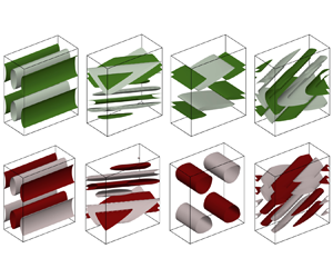
The results presented above imply that SOs and EOFs can be interpreted as representative resolvent modes. Indeed, the leading SOs and EOFs will often closely resemble ad hoc selections of dominant – across frequencies – resolvent forcing and response modes, as shown in figure 1 for a turbulent channel flow example. Implementation details for this example can be found in § 5.

Figure 1. Forcing and response resolvent modes at handpicked high-gain frequencies compared to the leading SOs and EOFs for mean-flow-linearized minimal channel flow at  $Re_\tau =185$. Real part of modes depicted as isosurfaces of wall-normal forcing and streamwise velocity response.
2.4. Gramian-based forcing and response modes
Although SOs and EOFs are usually explained as the structures that optimally contribute to and account for the sustained variance in stochastically excited flows, they also have an interesting deterministic interpretation (Farrell & Ioannou Reference Farrell and Ioannou2001). Specifically, the SOs and EOFs correspond to the most responsive forcings and the most receptive responses across all frequencies. This is formalized by deriving the SOs and EOFs as the solutions to the optimization problems presented below.
Let us first introduce the  $\mathcal {L}_2$-norm for signals $\boldsymbol {y}(t)$. This norm measures energy integrated over time, as follows:
 \begin{equation} \|\boldsymbol{y}(t)\|_{\mathcal{L}_2}^2=\int_0^\infty \|\boldsymbol{y}(t)\|_2^2 \,\mathrm{d}t=\frac{1}{2{\rm \pi}}\int_{-\infty}^\infty \|\hat{\boldsymbol{y}}(\omega)\|_2^2\,\mathrm{d}\omega =\|\hat{\boldsymbol{y}}(\omega)\|_{\mathcal{L}_2}^2,\end{equation}
where  $\hat {(\,\cdot\,)}$ denotes a Fourier-transformed variable, and the frequency domain expression follows from Plancherel's theorem.
In order to define our objective functions to be maximized, we consider the gain in the  $\mathcal {L}_2$-norm for signals. Moreover, the last equality in (2.10) implies that, in the $\mathcal {L}_2$ sense, optimizing energy amplification integrated over all frequencies is equivalent to optimizing energy growth integrated over all time.
Hence the most responsive forcing across all frequencies is the mode  $\boldsymbol {v}$ that, mapped through the resolvent, produces the most amplified response in the $\mathcal {L}_2$ sense and is found by maximizing the gain
 \begin{equation} \frac{\|\boldsymbol{H}({\rm i}\omega)\,\boldsymbol{v} \|^2_{\mathcal{L}_2}}{\|\boldsymbol{v}\|_2^2} = \frac{\|{\rm e}^{\boldsymbol{A}t}\,\boldsymbol{v} \|^2_{\mathcal{L}_2}}{\|\boldsymbol{v}\|_2^2} = \frac{\boldsymbol{v}^* \displaystyle\int\nolimits_0^\infty {\rm e}^{\boldsymbol{A}^*t}\,{\rm e}^{\boldsymbol{A}t} \,\mathrm{d}t \,\boldsymbol{v}}{\boldsymbol{v}^*\boldsymbol{v}} = \frac{\boldsymbol{v}^*\boldsymbol{W_o} \boldsymbol{v}}{\boldsymbol{v}^*\boldsymbol{v}}, \end{equation}
where the observability Gramian  $\boldsymbol {W_o}$ emerges naturally from expanding the norm definition. In fact, the cost function in the rightmost expression corresponds to a Rayleigh quotient, thus the optimizer is the leading eigenvector of $\boldsymbol {W_o}$, that is, the leading SO. Subsequent eigenvectors then solve for the next most responsive forcings. Although the association between the most observable modes and the most responsive forcings may seem counter-intuitive, these are the structures that generate the most energetic responses, and can therefore be most easily discerned from the time history of the state.
Now, the most receptive response across all frequencies is the mode  $\boldsymbol {v}$ that best aligns, in the $\mathcal {L}_2$ sense, with all possible responses, which are spanned by the columns of the resolvent, thus maximizing the gain
 \begin{equation} \frac{\|\boldsymbol{H}({\rm i}\omega)^*\,\boldsymbol{v} \|^2_{\mathcal{L}_2}}{\|\boldsymbol{v}\|_2^2} = \frac{\|{\rm e}^{\boldsymbol{A}^*t}\,\boldsymbol{v} \|^2_{\mathcal{L}_2}}{\|\boldsymbol{v}\|_2^2} = \frac{\boldsymbol{v}^* \displaystyle\int\nolimits_0^\infty {\rm e}^{\boldsymbol{A}t}\,{\rm e}^{\boldsymbol{A}^*t} \,\mathrm{d}t \,\boldsymbol{v}}{\boldsymbol{v}^*\boldsymbol{v}} = \frac{\boldsymbol{v}^*\boldsymbol{W_c} \boldsymbol{v}}{\boldsymbol{v}^*\boldsymbol{v}}, \end{equation}
where now a Rayleigh quotient with the controllability Gramian  $\boldsymbol {W_c}$ appears in the last expression. Thus the optimizer corresponds to its leading eigenvector, that is, the leading EOF. Again, subsequent eigenvectors then solve for the next most receptive responses in the same sense. The intuition behind the association between controllable modes and the most receptive responses lies in the fact that these are the states that the system is most easily steered to through the action of any input or forcing.
When working with modal decompositions of fluid flows (or dynamical systems in general), it is useful to think about the optimization problems being solved to provide physical interpretations for the modes. This has been particularly important for non-normal systems, where non-modal stability analyses have provided valuable insights regarding physical mechanisms for linear energy amplification (Schmid Reference Schmid2007). As we have shown, and summarize in table 1, the forcing and response modes produced by the Gramian eigenvectors are closely connected to those obtained from transient growth and resolvent analyses.
Table 1. Forcing and response modes for non-normal systems, and the optimization problems that they solve.

It is important to note that we have been using the Euclidean  $2$-norm to represent the energy of a state vector $\|\boldsymbol {v}\|_2^2$. It is often the case that a physically meaningful inner product considers a positive-definite weighting matrix $\boldsymbol {Q}$ so that the relevant metric is $\|\boldsymbol {v}\|_{\boldsymbol {Q}}^2=\boldsymbol {v}^*\boldsymbol {Qv}$. This weighting might account for integration quadratures or scaling of heterogeneous variables in multi-physics systems (Herrmann-Priesnitz et al. Reference Herrmann-Priesnitz, Calderón-Muñoz, Diaz and Soto2018a). However, in this scenario, one can modify the problem conveniently and easily to work with the Euclidean $2$-norm by taking the state as $\boldsymbol {Fv}$ and the dynamics as $\boldsymbol {F A F}^{-1}$, where $\boldsymbol {F}^*$ is the Cholesky factor of $\boldsymbol {Q}=\boldsymbol {F}^*\boldsymbol {F}$.
3. Interpolatory input and output projections
We begin this section by presenting the main motivation for input and output projections and their conventional definitions using orthogonal projectors. Next, we formally define the concept of interpolatory projectors. Finally, we introduce our proposed method and the ideas for its application in the context of flow control, which are the main contributions of this work.
3.1. Orthogonal input and output projections
The goal of input and output projections is to find projectors  $\mathbb {P}$ to produce low-rank approximations of either inputs or outputs, respectively, such that the input–output behaviour remains as close as possible to that of the original system of form (2.3a,b). In the case of input projections, the approximated dynamics is governed by
 \begin{equation} \frac{\mathrm{d} \tilde{\boldsymbol{x}}}{\mathrm{d} t}=\boldsymbol{A}\tilde{\boldsymbol{x}}+\boldsymbol{B}\mathbb{P}\boldsymbol{u}, \quad \tilde{\boldsymbol{y}} = \boldsymbol{C}\tilde{\boldsymbol{x}}, \end{equation}
and for the case of output projections, it is described by
 \begin{equation} \frac{\mathrm{d}\kern0.7pt \boldsymbol{x}}{\mathrm{d} t}=\boldsymbol{Ax}+\boldsymbol{Bu}, \quad \tilde{\boldsymbol{y}} = \mathbb{P}\boldsymbol{Cx}. \end{equation}
In both scenarios, we want the outputs  $\boldsymbol {y}(t)$ and $\tilde {\boldsymbol {y}}(t)$ for the original and projected systems to be close for a sequence of inputs $\boldsymbol {u}(t)$. We will consider the $\mathcal {L}_2$-norm for signals, introduced in (2.10), as our metric of choice, which measures energy integrated over time. Under this norm, the input projection error becomes
 \begin{align} \|\boldsymbol{y}(t)-\tilde{\boldsymbol{y}}(t)\|_{\mathcal{L}_2}^2&= \frac{1}{2{\rm \pi}}\int_{-\infty}^\infty \|\boldsymbol{G}({\rm i}\omega)\hat{\boldsymbol{u}}(\omega)-\boldsymbol{G}({\rm i}\omega)\,\mathbb{P}\,\hat{\boldsymbol{u}}(\omega)\|_2^2\, \mathrm{d}\omega \end{align}
 \begin{align} &= \frac{1}{2{\rm \pi}}\int_{-\infty}^\infty \|\boldsymbol{G}({\rm i}\omega)\,(\boldsymbol{I}-\mathbb{P})\,\hat{\boldsymbol{u}}(\omega)\|_2^2\,\mathrm{d}\omega, \end{align}
and the output projection error becomes
 \begin{align} \|\boldsymbol{y}(t)-\tilde{\boldsymbol{y}}(t)\|_{\mathcal{L}_2}^2 &= \frac{1}{2{\rm \pi}}\int_{-\infty}^\infty \|\boldsymbol{G}({\rm i}\omega)\,\hat{\boldsymbol{u}}(\omega)-\mathbb{P}\,\boldsymbol{G}({\rm i}\omega)\,\hat{\boldsymbol{f}}(\omega)\|_2^2\,\mathrm{d}\omega \end{align}
 \begin{align} &= \frac{1}{2{\rm \pi}}\int_{-\infty}^\infty \|(\boldsymbol{I}-\mathbb{P})\,\boldsymbol{G}({\rm i}\omega)\,\hat{\boldsymbol{u}}(\omega)\|_2^2\,\mathrm{d}\omega, \end{align}
where  $\boldsymbol {G}(s)=\boldsymbol {C}(s\boldsymbol {I}-\boldsymbol {A})^{-1}\boldsymbol {B}=\boldsymbol {C}\,\boldsymbol {H}(s)\,\boldsymbol {B}$ is the transfer function for the unprojected system (2.3a,b).
The values of  $\mathbb {P}$ that minimize the errors (3.3) and (3.4) depend on the class of inputs admitted and on the type of projector sought. The methods introduced by Dergham et al. (Reference Dergham, Sipp and Robinet2011a) and Rowley (Reference Rowley2005) seek orthogonal projectors to minimize the errors (3.3) and (3.4), respectively, for inputs that are impulses on every possible degree of freedom. Given an orthonormal set of vectors $\boldsymbol {V}=[\boldsymbol {v}_{1} \ \cdots \ \boldsymbol {v}_{r}]$, an orthogonal projector onto the column space of $\boldsymbol {V}$ is given by $\mathbb {P}_{\perp }=\boldsymbol {VV}^*$.
If such a rank- $r$ projector minimizes the input projection error (3.3), then the modes in $\boldsymbol {V}$ correspond to the most dynamically relevant inputs, that is, the response of the system can be well predicted when approximating $\boldsymbol {u}(t)\approx \mathbb {P}_{\perp }\,\boldsymbol {u}(t)= \boldsymbol {VV}^*\,\boldsymbol {u}(t)=\boldsymbol {V}\,\boldsymbol {d}(t)$, with $\boldsymbol {d}(t)\in \mathbb {C}^{r}$. In addition to the physical insight regarding the most responsive inputs, these modes can be leveraged to design spatially distributed actuators. Building actuators that are tailored to excite these modes results in a controller that can act along the most responsive directions in state space. The optimal basis for orthogonal input projection is given by the leading POD modes from adjoint impulse response simulations, which, in the case of full state inputs, are equivalent to the leading observable modes (Dergham et al. Reference Dergham, Sipp and Robinet2011a).
Similarly, if the output projection error in (3.4) is minimized, then  $\boldsymbol {V}$ spans the subspace of the most receptive measurements. In this case, the modes in $\boldsymbol {V}$ allow for a low-dimensional representation of the output in terms of mode amplitudes, that is, $\boldsymbol {y}(t)\approx \mathbb {P}_{\perp }\,\boldsymbol {y}(t)= \boldsymbol {VV}^*\,\boldsymbol {y}(t)=\boldsymbol {V}\,\boldsymbol {a}(t)$, with $\boldsymbol {a}(t)\in \mathbb {C}^{r}$. The optimal basis for orthogonal output projection is given by the leading POD modes from direct impulse response simulations, which, in the case of full state outputs, are equivalent to the leading controllable modes (Rowley Reference Rowley2005; Holmes et al. Reference Holmes, Lumley, Berkooz and Rowley2012).
Furthermore, in this work we are concerned with fluid flows that can be forced anywhere and measured everywhere, that is, the system has full state inputs and outputs simultaneously. Recall that if this is the case, then the transfer function becomes the resolvent operator  $\boldsymbol {G}(s)=\boldsymbol {H}(s)$. In this scenario, the optimal bases that minimize (3.3) and (3.4) are comprised of flow structures that coincide with the leading SOs and EOFs, and can be interpreted as the most responsive forcings and receptive responses, respectively.
3.2. Interpolatory projectors
We have presented the idea of using projectors to produce low-rank approximations of inputs and outputs, or forcings and responses in dynamical systems of the form in (2.1) with full state inputs and outputs. The optimal orthogonal projectors that minimize the errors (3.3) and (3.4) in that case use the leading SOs and EOFs as bases. Here, we define another kind of projector – an interpolatory projector – that, as we show later, is useful practically for sensor and actuator placement and open-loop control.
An interpolatory projector is an oblique projector with the special property of preserving exactly certain entries in any vector upon which it acts. These entries are referred to as interpolation points, thus justifying the name, which was first introduced in Chaturantabut & Sorensen (Reference Chaturantabut and Sorensen2010) and later adopted by more recent work (Sorensen & Embree Reference Sorensen and Embree2016; Gidisu & Hochstenbach Reference Gidisu and Hochstenbach2021).
Definition 3.1 Given a full-rank matrix  $\boldsymbol {V}\in \mathbb {R}^{n\times r}$ and a set of distinct indices $\boldsymbol {\gamma }\in \mathbb {N}^r$, the interpolatory projector for $\boldsymbol {\gamma }$ onto the column space of $\boldsymbol {V}$ is
 \begin{equation} \mathbb{P}_{:}\equiv \boldsymbol{V}(\boldsymbol{P}^{\rm{T}} \boldsymbol{V})^{{-}1}\boldsymbol{P}^{\rm{T}}, \end{equation}
provided that  $\boldsymbol {P}^{\rm {T}} \boldsymbol {V}$ is invertible, where $\boldsymbol {P}=[\boldsymbol {e}_{{\gamma }_1} \ \cdots \boldsymbol {e}_{{\gamma }_r}] \in \mathbb {R}^{n\times r}$ contains $r$ columns of the identity matrix given by $\boldsymbol {\gamma }$.
The matrix  $\boldsymbol {P}$ is a sparse matrix, referred to as the sampling matrix because it samples the entries given by the indices $\boldsymbol {\gamma }$ of any vector $\boldsymbol {x}\in \mathbb {R}^n$ upon which it acts, that is, $\boldsymbol {P}^{\rm {T}}\boldsymbol {x}=\boldsymbol {x}(\boldsymbol {\gamma })$. Just like an orthogonal projector $\mathbb {P}_{\perp }=\boldsymbol {VV}^{\rm {T}}$, when $\mathbb {P}_{:}$ is applied to a vector, the result is in the column space of $\boldsymbol {V}$. However, $\mathbb {P}_{:}$ is an oblique projector, and it also has the following distinct property: for any $\boldsymbol {x}\in \mathbb {R}^n$,
 \begin{equation} (\mathbb{P}_{:}\boldsymbol{x})(\boldsymbol{\gamma})=\boldsymbol{P}^{\rm{T}}\mathbb{P}_{:}\boldsymbol{x}=\boldsymbol{P}^{\rm{T}}\boldsymbol{V}(\boldsymbol{P}^{\rm{T}} \boldsymbol{V})^{{-}1} \boldsymbol{P}^{\rm{T}}\boldsymbol{x} = \boldsymbol{P}^{\rm{T}}\boldsymbol{x} = \boldsymbol{x}(\boldsymbol{\gamma}), \end{equation}
so the projected vector  $\mathbb {P}_{:}\boldsymbol {x}$ matches $\boldsymbol {x}$ in the entries indicated by $\boldsymbol {\gamma }$. These entries are known as the interpolation or sampling points, and are determined by the non-zero entries in the sampling matrix. A simple example of interpolatory projection is presented in Appendix A.
3.3. Proposed method
For our interpolatory input and output projections, we take the leading SOs and EOFs as the basis  $V$, respectively. It is important to note that these projectors are sub-optimal with respect to (3.3) and (3.4), and therefore will never show better performance (under these metrics) than the orthogonal projectors of the same rank built with the same bases. Furthermore, the choice of the sampling locations, or equivalently the design of $\boldsymbol {P}$, is critical for the performance of the interpolatory projection to approximate that of the orthogonal one. In addition, when using the leading SOs or EOFs in $\boldsymbol {V}$, the interpolation points that result in small projection errors are physically interesting, since they represent responsive or receptive spatial locations, respectively. However, finding the optimal sampling matrix that minimizes the projection error for a given basis $\boldsymbol {V}$ requires a brute force search over all possible sampling location combinations. While this can be achieved for small-scale systems (Chen & Rowley Reference Chen and Rowley2011), with $n\sim {O}(10^4)$ at the time of writing, the computational cost makes it intractable in higher dimensions. Alternatively, there are several fast greedy algorithms that can be used to approximate the optimal sensor locations, avoiding the combinatorial search. In the context of reduced-order modelling, the empirical and discrete empirical interpolation methods, EIM (Barrault et al. Reference Barrault, Maday, Nguyen and Patera2004) and DEIM (Chaturantabut & Sorensen Reference Chaturantabut and Sorensen2010), were developed to find locations to interpolate nonlinear terms in a high-dimensional dynamical system, which is known as hyper-reduction. An even simpler and equally efficient approach is the Q-DEIM algorithm, introduced by Drmac & Gugercin (Reference Drmac and Gugercin2016), that leverages the pivoted QR factorization to select the sampling points. Manohar et al. (Reference Manohar, Brunton, Kutz and Brunton2018) showed that this is also a robust strategy for sparse sensor placement for state reconstruction on a range of applications. Here, we adhere to this method because it provides near-optimal interpolation points and is simple to implement by leveraging the pivoted QR factorization available in most scientific computing software packages. The pseudo-code for this greedy sensor selection strategy, adapted from Manohar et al. (Reference Manohar, Brunton, Kutz and Brunton2018), is shown in Algorithm 1, where we use Matlab's array slicing notation.
Algorithm 1 Greedy sensor selection using pivoted QR (Manohar et al. 2018)

Therefore, the approach used to build  $\boldsymbol {P}$ for our interpolatory input or output projections consists in taking a pivoted QR factorization of the transpose of the basis $V$, which is comprised of the leading either SOs or EOFs, respectively. Then the first $r$ QR pivots correspond to the sampling points, or sensor locations, which we will refer to as tailored sensors since they depend solely on the corresponding $\boldsymbol {V}$, and are therefore tailored specifically to that basis (Manohar et al. Reference Manohar, Brunton, Kutz and Brunton2018).
Combining the SOs and EOFs with the pivoted QR factorization for sampling point selection, we obtain an equation-driven framework for interpolatory input and output projections that is easy to implement. In the following, we explain how this approach can be leveraged for several control-related tasks.
3.4. Sparse sensor and actuator placement
The leading SOs span the subspace of the dominant forcings for response prediction. Using an interpolatory projector, these dominant forcings can be approximated as  $\boldsymbol {f}(t)\approx \mathbb {P}_{:}\,\boldsymbol {f}(t)=\boldsymbol {V}(\boldsymbol {P}^{\rm {T}} \boldsymbol {V})^{-1} \boldsymbol {P}^{\rm {T}}\,\boldsymbol {f}(t)=\boldsymbol {V}(\boldsymbol {P}^{\rm {T}} \boldsymbol {V})^{-1}\,\boldsymbol {d}(t)$, where now $\boldsymbol {d}$ corresponds to the entries of $\boldsymbol {f}$ at the $r$ interpolation points. This means that we can approximate the dynamically relevant parts of the forcing from sparse sensor measurements, and if a model of the dynamics is available, predict the response of the system. Moreover, the interpolation points also make attractive open-loop actuator locations to act on the SOs and mitigate the disturbances with the largest impact on the dynamics. Similarly, using the EOFs, we can reconstruct the response $\boldsymbol {x}(t)\approx \mathbb {P}_{:}\,\boldsymbol {x}(t)=\boldsymbol {V}(\boldsymbol {P}^{\rm {T}} \boldsymbol {V})^{-1} \boldsymbol {P}^{\rm {T}}\,\boldsymbol {x}(t)=\boldsymbol {V}(\boldsymbol {P}^{\rm {T}} \boldsymbol {V})^{-1}\,\boldsymbol {a}(t)$ from sparse sensor measurements $\boldsymbol {a}$ corresponding to the entries of $\boldsymbol {x}$ at the $r$ interpolation points.
Balanced modes, corresponding to the most jointly controllable and observable states of a linear dynamical system (Moore Reference Moore1981; Rowley & Dawson Reference Rowley and Dawson2017), have also been leveraged for sensor and actuator placement by Manohar et al. (Reference Manohar, Kutz and Brunton2021). However, that work was focused on feedback control, whereas here we are proposing sensors for forcing or response reconstruction and actuators for open loop control. Although balanced modes may also seem like attractive choices of bases to build input and output projectors, the subspaces that they span are sub-optimal for projection in terms of the errors (3.3) and (3.4), since the balancing implies a trade-off between observability and controllability. Therefore, for the tasks presented in this work, that rely on input and output projections, the eigenvectors of the Gramians are more principled choices of bases. This way, the resulting interpolatory projectors are approximating the optimal orthogonal projectors.
3.5. Partial disturbance feedforward control
Disturbance feedforward control is an open-loop control strategy that uses measurements of the disturbances to a system and a model of its dynamics to determine a sequence of control inputs with the objective of mitigating the effect of disturbances. This strategy is used typically to reject low-frequency, high-amplitude disturbances and perform aggressive reference tracking, in combination with a feedback controller that attenuates high-frequency sensor noise and compensates for model uncertainty (Bade et al. Reference Bade, Hanson, Belson, Naguib, Lavoie and Rowley2016; Papadakis, Lu & Ricco Reference Papadakis, Lu and Ricco2016; Williams & King Reference Williams and King2018; Tol, Kotsonis & De Visser Reference Tol, Kotsonis and De Visser2019; Herrmann et al. Reference Herrmann, Brunton, Pohl and Semaan2022). Consider a linear dynamical system
 \begin{equation} \frac{\mathrm{d}\kern0.7pt \boldsymbol{x}}{\mathrm{d} t}=\boldsymbol{Ax}+\boldsymbol{w}+\boldsymbol{Bu}, \quad \boldsymbol{y}=\boldsymbol{Cw},\end{equation}
that is forced simultaneously by exogenous disturbances  $\boldsymbol {w}$ and the control actuation term $\boldsymbol {Bu}$, with $\boldsymbol {u}\in \mathbb {C}^p$ and $\boldsymbol {B}\in \mathbb {C}^{n\times p}$, where $\boldsymbol {y}=\boldsymbol {Cw}$ are measurements of the disturbances through the linear mapping $\boldsymbol {C}\in \mathbb {C}^{q\times n}$. This is a particular case of the disturbance feedforward control problem presented in Doyle et al. (Reference Doyle, Glover, Khargonekar and Francis1988) with no feedback, where the error signal $\boldsymbol {z}=\boldsymbol {x}$ is just the state. Therefore, for a given set-up, an optimal control law can be derived within the framework of $\mathcal {H}_2$ control (Doyle et al. Reference Doyle, Glover, Khargonekar and Francis1988; Skogestad & Postlethwaite Reference Skogestad and Postlethwaite2005). However, we consider the joint problem of designing simultaneously the actuation matrix $\boldsymbol {B}$, the measurement matrix $\boldsymbol {C}$ and a simple control law with a constant gain matrix $\boldsymbol {u}=-\boldsymbol {Ky}$, with the aim of mitigating only the most meaningful disturbances. Substituting the control law in (3.7a,b), the controlled system dynamics becomes
 \begin{equation} \frac{\mathrm{d}\kern0.7pt \boldsymbol{x}}{\mathrm{d} t}=\boldsymbol{Ax}+\boldsymbol{f}, \quad \boldsymbol{f} = \left(\boldsymbol{I}-\boldsymbol{BKC}\right)\boldsymbol{w},\end{equation}
where the system is forced by the effective forcing  $\boldsymbol {f}$. Now we want to find a combination of actuators $\boldsymbol {B}$, disturbance sensors $\boldsymbol {C}$ and gain $\boldsymbol {K}$ that minimizes the effect of $\boldsymbol {f}$ on the response of the system. This is achieved if $(\boldsymbol {I}-\boldsymbol {BKC})$ projects $\boldsymbol {w}$ onto the least responsive disturbances, or equivalently, if $\boldsymbol {BKC}$ projects onto the most responsive disturbances, given by the leading SOs of the system (3.8a,b). In other words, the sensors, control gains and actuators can be selected conveniently so that the matrix product of $\boldsymbol {B}$, $\boldsymbol {K}$ and $\boldsymbol {C}$ produces an orthogonal or interpolatory input projector. Note that this approach only partially mitigates the disturbances, which is why we refer to it as partial disturbance feedforward control.
This approach is particularly attractive for noise-amplifier systems, where a few preferred forcing structures are responsible for most of the energy sustained by the response (Dergham et al. Reference Dergham, Sipp and Robinet2011a, Reference Dergham, Sipp and Robinet2013). In § 4, we demonstrate the performance of partial disturbance feedforward control on a stochastically forced linear system considering different types of sensors and actuators.
Furthermore, the proposed approach may also prove to be interesting in the context of turbulent flows. Specifically, for wall-bounded turbulent flows, the SOs of the mean-flow linearization are expected to be an efficient basis for input projection because of their behaviour as selective noise amplifiers (Dergham et al. Reference Dergham, Sipp and Robinet2013). However, the effect of control inputs would cause mean-flow deformation. Whether or not the actuators designed based on the SOs of the uncontrolled flow would remain effective when control is in place has yet to be investigated. This will be the subject of future research and is outside the scope of the present work.
4. Leveraging forcing modes
In this section, we present three numerical examples detailing how orthogonal and interpolatory input projections relying on Gramian-based forcing modes can be leveraged. First, in § 4.1 we show how orthogonal input projection is able to identify the most responsive disturbances to predict accurately the response of the system using a low-dimensional forcing. Building on this, in § 4.2 we use interpolatory input projection to approximate the dynamically relevant disturbances from sparse measurements of the forcing field. To close this section, in § 4.3 we test both kinds of input projectors to perform partial disturbance feedforward control and mitigate the effect of the most responsive forcing with different sensor and actuator configurations. Our test bed is the linearized complex Ginzburg–Landau equation, which is a typical model for instabilities in spatially evolving flows. The semi-discretized system is governed by the linear operator
 \begin{equation} \boldsymbol{A} ={-}\nu \boldsymbol{D}_x + \gamma \boldsymbol{D}_x^2 + \mu(x),\end{equation}
where  $x$ is the spatial coordinate, and $\boldsymbol {D}_x$ and $\boldsymbol {D}^2_x$ are the first- and second-order spatial differentiation matrices with homogeneous boundary conditions at $x\rightarrow \pm \infty$. We choose a quadratic spatial dependence for the parameter $\mu (x)=(\mu _0-c_{\mu }^2)+({\mu _2}/{2})x^2$ that has been used previously by several authors (Bagheri et al. Reference Bagheri, Henningson, Hoepffner and Schmid2009b; Chen & Rowley Reference Chen and Rowley2011; Towne, Schmidt & Colonius Reference Towne, Schmidt and Colonius2018). The other parameters are set to $\mu _0=0.23$, ${\mu _2=-0.01}$, $\nu =2+0.4{\rm i}$ and $\gamma =1-{\rm i}$ as in Towne et al. (Reference Towne, Schmidt and Colonius2018), giving rise to linearly stable dynamics. As in Bagheri et al. (Reference Bagheri, Henningson, Hoepffner and Schmid2009b), we use spectral collocation based on Gauss-weighted Hermite polynomials to build the differentiation matrices $\boldsymbol {D}_x$ and $\boldsymbol {D}^2_x$, and the integration quadrature. The spatial coordinate is discretized into $n=220$ collocation points, and the domain is truncated to $x\in [-85,85]$, which is sufficient to enforce the far-field boundary conditions. The observability Gramian considering full state inputs and outputs is computed using readily available routines that solve the corresponding Lyapunov equation (2.5a).
Throughout the examples, band-limited white noise disturbances  $\boldsymbol {f}(t)$ are generated, several input projectors $\mathbb {P}$ are built, and the responses of the system to $\boldsymbol {f}(t)$ and to the projected forcings $\mathbb {P}\boldsymbol {f}(t)$ are compared. Simulations are carried out by integrating numerically for $10^4$ time units, and the results are recorded every $\Delta t=0.5$ time units for post-processing. Every time step, the forcing is generated on a uniform spatial grid of $80$ points as a vector of random complex numbers with amplitudes drawn from a normal distribution and phases drawn from a uniform distribution, which is then mapped onto the non-uniform spatial grid via spline interpolation.
4.1. Most responsive disturbances
For the set of parameters used, the linearized complex Ginzburg–Landau equation is known to behave as a selective amplifier of disturbances (Bagheri et al. Reference Bagheri, Henningson, Hoepffner and Schmid2009b). When forced with white noise, the dynamics of the system filters disturbances and generates a response where most of the energy is contained in coherent structures, as shown in figure 2(a). This implies that, among all possible ways to excite the system, there are a few preferred forcing patterns that are dynamically relevant and have a dominant effect on the produced response.

Figure 2. (a) Response of the linearized complex Ginzburg–Landau equation to white noise forcing. The system behaves as a selective disturbance amplifier. (b) Two bases of representative forcing modes are used to build orthogonal input projectors: the leading forcing POD modes computed from snapshots of the disturbances, and the leading SOs. (c) Projected forcings and their induced responses using  $20$ forcing POD modes versus $3$ SOs. (d) Normalized input projection error as a function of the projector rank $r$. The real part is displayed for forcing, response and mode plots. These findings follow directly from the work of Dergham et al. (Reference Dergham, Sipp and Robinet2011a).
We build orthogonal projectors onto two different subspaces, spanned by the bases  $\boldsymbol {V}$ shown in figure 2(b), that one might consider when seeking low-rank approximations of the forcing. For the first subspace, we gather snapshots of the forcing, perform POD on those snapshots, and retain the leading $r$ forcing POD modes as our basis to build a rank- $r$ projector. The second subspace is the one spanned by the leading $r$ eigenvectors of the observability Gramian. The projection of the forcing onto these subspaces, and the response of the system to the projected forcings, are shown in figure 2(c) for $r=20$ POD modes and $r=3$
$r=3$  $\boldsymbol {W_o}$ eigenmodes.
The projected forcing using POD resembles closely the original forcing, which is expected since POD provides the optimal low-rank approximation based on empirical observations. Despite this, the response is predicted more accurately using the input projection onto the SOs, even when using just  $3$ modes compared to the $20$ used for the POD-based projection, as shown in figure 2(c). More quantitatively, the error in the response prediction, measured by the normalized $\mathcal {L}_2$-norm, is always lower for the same forcing projection rank $r$, and decreases much more rapidly for low-rank approximations, as shown in figure 2(d).
This performance gap is expected since the POD modes of the disturbance field, albeit optimal at reconstructing the observed disturbances, are completely agnostic to the dynamics of the system. The purpose of the comparison is to highlight the dynamical significance of the SOs as the most responsive disturbances, providing a subspace for input projection that is optimal for response prediction. We remark that the findings presented in this subsection are not new since they follow directly from the application of the method developed by Dergham et al. (Reference Dergham, Sipp and Robinet2011a).
4.2. Sensor placement for prediction
Using interpolatory input projection, the most responsive disturbances buried within white noise forcing can be exposed successfully from sparse sensor measurements, as shown in figure 3(a) for the case of  $8$ sensors. The projected forcing captures the dynamically relevant parts of the disturbances, allowing for an accurate prediction of the energetic coherent structures in the response, as also shown in figure 3(a). Moreover, the error induced by the interpolatory projection on the response prediction rapidly approaches the error induced by an orthogonal projector, built using the same basis, as the basis size increases, as shown in figure 3(b). The spatial locations found for the sensors, tailored to the eigenvectors of $\boldsymbol {W_o}$, resemble closely the optimal placements computed by Chen & Rowley (Reference Chen and Rowley2011). However, our approach circumvents solving the computationally expensive optimization problem presented in that work by using the pivoted QR method. Furthermore, the sensor locations found are also similar to those found by Manohar et al. (Reference Manohar, Kutz and Brunton2021), which is expected since those were tailored to the adjoint balanced modes, which span almost the same subspace as the eigenvectors of the observability Gramian for this particular case. Importantly, in that and other previous works, the sensor placement was optimized for feedback control, whereas here, sensors aim to reconstruct the disturbance field to use it for prediction. As discussed in § 3, for this purpose, balanced modes are sub-optimal and SOs are the optimal choice.

Figure 3. (a) Forcing applied to the linearized complex Ginzburg–Landau equation and its induced response compared to an interpolatory projection of the forcing and its induced response. The projector interpolates the forcing in the span of the leading  $r=8$ SOs from measurements at $r=8$ spatial locations (sensors). (b) Normalized input projection error using interpolatory (dashed) and orthogonal (solid) projectors as a function of the projector rank $r$. (c) Sensor locations as a function of the size of the basis used for projection. Sampling points are selected using pivoted QR, as in Manohar et al. (Reference Manohar, Brunton, Kutz and Brunton2018), and are therefore tailored to the basis of SOs. Plots show the real parts of forcings and responses.
4.3. Open-loop control design
Here, we consider the application of the partial disturbance feedforward control approach described in § 3 to the linearized complex Ginzburg–Landau equation subject to white noise disturbances. This strategy leverages the concept input projections to address only the most meaningful disturbances. With this strategy in mind, we design three feedforward controllers considering different restrictions on the allowable sensors and actuators.
First, we assume that we have access to full disturbance measurements, that is,  $\boldsymbol {C}=\boldsymbol {I}$, and that spatially distributed (body forcing) actuators are feasible. We design our actuators to excite directly the most responsive disturbances, that is, $\boldsymbol {B}=\boldsymbol {V}$, with $\boldsymbol {V}$ containing the leading SOs. Therefore, choosing the gain to be $\boldsymbol {K}=\boldsymbol {V}^*$ results in $\boldsymbol {BKC}$ being the optimal orthogonal input projector. Considering $r=10$ distributed actuators, the feedforward controller is able to successfully reject disturbances by projecting-out the components that would cause the most energetic response, as shown in figure 4(b). More precisely, a $97\,\%$ reduction in the $\mathcal {L}_2$-norm of the fluctuations is achieved.

Figure 4. (a) Feedforward control strategy to reject disturbances in the linearized complex Ginzburg–Landau equation. The control actuation and the response of the controlled system are shown for three sensor and actuator configurations: (b) full disturbance measurements and  $10$ spatially distributed (body forcing) actuators; (c) $10$ point sensors and $10$ spatially distributed actuators; and (d) $10$ localized sensors and actuators. Plots for the forcing, control actuations and responses display the real parts of these fields.
For a second case, we allow only pointwise measurements of the disturbances, that is,  $\boldsymbol {C}=\boldsymbol {P}^{\rm {T}}$, and still consider spatially distributed actuators. Choosing our actuators to be $\boldsymbol {B}=\boldsymbol {V}$ means that the gain $\boldsymbol {K}=(\boldsymbol {P}^{\rm {T}}\boldsymbol {V})^{-1}$ makes $\boldsymbol {BKC}$ an interpolatory input projector. In this scenario, the full disturbance field is interpolated from sparse sensors, and then the actuators attempt to cancel out the components that would lead to the most energetic response. Using $r=10$ spatially distributed actuators and $10$ point sensors, selected via pivoted QR, the feedforward controller has only slightly lower performance than when using full measurements, as shown in figure 4(c). Specifically, a $93\,\%$ reduction in the $\mathcal {L}_2$-norm of the fluctuations is obtained in this case.
Finally, we examine a more realistic scenario where only spatially localized sensors and actuators are allowed. Specifically, we consider  $\boldsymbol {B}=\tilde {\boldsymbol {P}}$ and $\boldsymbol {C}=\tilde {\boldsymbol {P}}^{\rm {T}}$, where, rather than $r$ columns of the identity as in $\boldsymbol {P}$, the columns of $\tilde {\boldsymbol {P}}$ are given by discretized Gaussian functions
 \begin{equation} \exp\left( -\frac{\left(x-x_j \right)^2}{2\sigma^2}\right), \quad j=1, \dots, r, \end{equation}
localized at sampling points  $x_j$, where we choose $\sigma =0.6$. Using a control gain $\boldsymbol {K}=(\tilde {\boldsymbol {P}}^{\rm {T}}\tilde {\boldsymbol {P}})^{-1}$, the actuation then attempts to cancel out directly the disturbances measured in the regions localized around the sampling points. We hypothesize that the optimal sensor locations for response prediction are also good for actuator placement, since they correspond to the optimal locations to interpolate the most responsive forcings. Therefore, leveraging the first $r=10$ SOs, we use pivoted QR to select $10$ sampling points to place disturbance sensors and actuators. The resulting controller has a reasonable disturbance rejection performance, as shown in figure 4(d). In this case, an $89\,\%$ reduction in the $\mathcal {L}_2$-norm of the fluctuations is achieved.
5. Leveraging response modes
In this section, we present numerical examples detailing how the orthogonal and interpolatory output projections can be leveraged to identify the most receptive perturbations of a dynamical system, and to reconstruct its state from sparse sensor measurements. As a test bed system, we use a minimal channel flow at  $Re_{\tau }=185$. This corresponds to a pressure-driven turbulent flow, governed by the incompressible Navier–Stokes equations, in a doubly periodic plane channel. The domain size is $1.83\times 2\times 0.92$ dimensionless length units along the $x$,
$x$,  $y$ and $z$ coordinates that indicate the streamwise (periodic), wall-normal and spanwise (periodic) directions, respectively. For Reynolds number $Re=4200$, based on the channel half-height $h$ and the centreline velocity for the laminar parabolic profile $U_{c,{lam}}$, leading to $Re_{\tau }=185$, this is the smallest domain that is able to sustain turbulence, and it is known as a minimal flow unit (Jiménez & Moin Reference Jiménez and Moin1991).
We use the spectral code Channelflow (Gibson, Halcrow & Cvitanović Reference Gibson, Halcrow and Cvitanović2008; Gibson Reference Gibson2014) to perform direct numerical simulations (DNS). The code uses Chebyshev and Fourier expansions of the flow field in the wall-normal and horizontal directions, and a third-order Adams–Bashforth backward differentiation scheme for the time integration. We find that a grid with  $32\times 101\times 16$ (after de-aliasing) in $x$,
$x$,  $y$ and $z$, and a time step $0.005$ time units, are sufficient to discretize the domain and keep the CFL number below $0.55$, for the cases studied. The flow is initialized from a random perturbation of the laminar profile, simulated for $10^4$ time units (based on $h/U_{c,{lam}}$) until transients have died out and statistical stationarity is reached, then velocity field snapshots are saved every $0.2$ time units for an additional $1.5\times 10^4$ time units, which is enough to get converged statistics. The streamwise velocity for a typical flow field snapshot is shown in figure 5(b).

Figure 5. (a) Snapshots of minimal channel flow at  $Re_{\tau }=185$ projected onto subspaces spanned by the leading $r$ POD modes (top) and the leading $r$ EOFs of the mean-flow-linearized operator (bottom). (b) A typical DNS snapshot. The colour map shows streamwise velocity. (c) Streamwise and wall-normal root-mean-square (r.m.s.) velocity profiles of the projected snapshots at various projection ranks. The left-hand plots (green curves) correspond to POD-based projections, and the right-hand plots (purple curves) to EOF-based projections. (d) Normalized output projection error as a function of the projector rank $r$. POD modes span the optimal (in the $\mathcal {L}_2$ sense) linear subspace and therefore represent the lower bound for this error.
The mean flow is computed from the DNS snapshots and used to build the mean-flow-linearized operator with an in-house code based on the Orr–Sommerfeld/Squire formulation. The code uses Chebyshev spectral collocation to discretize the wall-normal direction with the same grid used in the DNS. The linearized operator is built for every wavenumber tuple in the range resolved by the DNS, and the controllability Gramian, considering full state inputs and outputs, is computed solving the corresponding Lyapunov equation (2.5b) with available routines. Global EOFs (eigenvectors of  $\boldsymbol {W_c}$) are computed by taking the inverse Fourier transform of the local EOFs obtained for every wavenumber tuple and ordering them according to their energy (eigenvalues of $\boldsymbol {W_c}$).
Orthogonal and interpolatory projections of velocity fluctuation snapshots from the DNS are investigated. The EOFs, arising from the mean-flow linearization, and POD modes, spanning the optimal linear subspace, are compared as bases for the projections. To compute the POD modes, the DNS dataset is augmented with reflections of the snapshots with respect to the midplanes in the  $y$ and $z$ directions to enforce the corresponding symmetries. We then perform a randomized SVD (Halko, Martinsson & Tropp Reference Halko, Martinsson and Tropp2011) aiming at the leading $800$ POD modes using a Gaussian random matrix with $1000$ columns and without power iterations.
5.1. Most receptive perturbations
We examine the suitability of the EOFs and POD modes as bases  $\boldsymbol {V}$ for the dominant response subspace. We build rank- $r$ orthogonal projectors from the leading $r$ elements in these bases, and use them to project the DNS snapshots. Qualitatively, both POD modes and $\boldsymbol {W_c}$ eigenmodes seem to capture the main coarse features in the flow with a rank $100$ projection and further details as $r$ increases, as shown in figure 5(a) for the streamwise velocity.
Second-order statistics of the velocity fluctuations are approached by those obtained for the projected snapshots as the rank of the projector increases with both bases, as shown in figure 5(c). However, there is a slower convergence for the Gramian-based projection. Specifically, although the Gramian eigenmodes capture reasonably the peak in the root-mean-square (r.m.s.) profiles, a higher number of modes is required to resolve properly the statistics close to the wall and near the channel centre.
More quantitatively, the response projection error, measured by the normalized  $\mathcal {L}_2$-norm, drops faster with increasing $r$ and is always lower when using POD modes, as shown in figure 5(d). This is expected because POD modes span the optimal linear subspace in the $\mathcal {L}_2$ sense and therefore represent the lower bound for the response projection error. Nevertheless, for this system, the error of the projection onto the EOFs follows this lower bound closely. Importantly, this performance is achieved without any data snapshots and requires only knowledge of the mean flow, as opposed to the long sequence of high-fidelity snapshots needed to obtain converged POD modes. These results are not surprising since resolvent analysis has been very successful to model wall-bounded turbulent flows (McKeon Reference McKeon2017), and as explained in § 2, the EOFs and the combination of all resolvent response modes at all frequencies span the same subspace.
5.2. Sensor placement for reconstruction
We now examine the performance of interpolatory projectors to reconstruct velocity fluctuations in the minimal channel flow from sparse sensor measurements. Again, sensor locations are selected using the pivoted QR approach from Manohar et al. (Reference Manohar, Brunton, Kutz and Brunton2018), and are thus tailored to the specific basis used. The sensor placement distribution reveals the spatial regions that are most informative to reconstruct the dominant coherent structures. Since the state vector of the system contains the three velocity components, sensors are also selecting which component to measure.
Leveraging both of our bases, of POD modes and EOFs, we find that sensors accumulate towards the walls as more of them are added, as shown in figure 6(a). A detailed view of the sensor distribution in the wall-normal direction, presented in figure 6(b), reveals that most of the sensors tailored to the EOFs are positioned closer to the wall and fall within the buffer region. For both bases, the great majority of the sensors measure streamwise velocity, which is expected since that is the most energetic component. Interestingly, there is more variety in the sensors tailored to the POD basis, including more measurements of the spanwise and wall-normal velocities, as shown in figure 6(b).

Figure 6. (a) Spatial locations of sensors designed to reconstruct the velocity fluctuations in minimal channel flow at  $Re_{\tau }=185$. Sensors selected via pivoted QR (Manohar et al. Reference Manohar, Brunton, Kutz and Brunton2018) are tailored to the leading $r$ POD modes (top) and the leading $r$ EOFs (bottom). Sensors can measure streamwise (black circles), spanwise (cyan squares) or wall-normal (magenta triangles) velocity components. (b) Mean velocity profile in wall units (bottom) and distribution of sensors in the wall-normal direction for $r=800$ using POD (top) and EOFs (middle). (c) Normalized output projection error as a function of the projector rank $r$ (left) and of the percentage of sensors over the total number of state variables (right). Three interpolatory projectors are considered for each basis, using: $r$ tailored sensors complemented with $2r$ random sensors (dashed), $3r$ random sensors (dash-dotted), and all possible sensors (solid), which is equivalent to an orthogonal projector.
A total of six projectors are built, three for each basis, and the reconstruction  $\mathcal {L}_2$ error over the entire sequence of DNS snapshots is evaluated as a function of the projection rank $r$, as shown in figure 6(c). Considering the leading $r$ elements in each basis, we build interpolatory output projectors using $r$ tailored sensors complemented with an additional $2r$ random sensors. Because this is a high-dimensional system with a total of $n\approx 1.6\times 10^5$ states, complementing tailored sensors with random ones is a simple strategy to improve the resulting reconstruction that was suggested in the work of Manohar et al. (Reference Manohar, Brunton, Kutz and Brunton2018). This is implemented by simply taking the leading $2r$ columns of a matrix containing all remaining possible sensors after a random column permutation. These columns are then concatenated to the sampling matrix $\boldsymbol {P}$ used to build the projector. For the sake of comparison, we also build interpolatory projectors using $3r$ random sensors and orthogonal projectors for the subspaces spanned by the POD modes and by the eigenvectors of $\boldsymbol {W_c}$. Orthogonal projectors provide the lower bound in reconstruction error for interpolatory projectors onto the same subspace. Leveraging the EOFs, the reconstruction using tailored sensors explains a large portion of the energy in the flow field, and even with random sensors, $50\,\%$ of the energy is captured from measurements of $1.5\,\%$ of the state variables, as shown in figure 6(c). Furthermore, this is achieved in a data-free manner, requiring only knowledge of the mean flow.
6. Conclusions
The main contribution of this work is the introduction of interpolatory input and output projections along with numerical examples that demonstrate their use for sensor and actuator placement and open-loop control. The presented approach leverages the leading stochastic optimals (SOs) and empirical orthogonal functions (EOFs) that are known to be optimal bases for orthogonal input and output projections for linear stable systems (Rowley Reference Rowley2005; Dergham et al. Reference Dergham, Sipp and Robinet2011a). This is also motivated by the connection between SOs and EOFs and resolvent forcing and response modes, for which we offer a brief review. The sampling points for our interpolatory projections are selected conveniently using the fast greedy algorithm developed by Manohar et al. (Reference Manohar, Brunton, Kutz and Brunton2018).
The SOs provide an orthonormal basis of forcing modes that are ordered hierarchically by their contribution to the response. This means that the response of a system that is being excited by high-dimensional disturbances can be approximated by the response to the projection of those disturbances onto the leading SOs. In fact, if all disturbances are equally likely, then these modes provide the optimal basis of the forcing for response prediction (Dergham et al. Reference Dergham, Sipp and Robinet2011a). Although this is certainly not the case for turbulent flows, where there are preferred disturbances because nonlinearity provides coloured forcing, we still expect these modes to provide an excellent, albeit sub-optimal, forcing basis for highly non-normal systems. This is supported by the bulk of resolvent literature for the case of wall-bounded turbulence (McKeon Reference McKeon2017), since resolvent forcing modes and the SOs span the same subspaces. For instance, Bae, Lozano-Duran & McKeon (Reference Bae, Lozano-Duran and McKeon2021) showed that turbulence in a minimal channel flow is inhibited if the leading resolvent forcing mode (corresponding to the most dangerous frequency) is projected out of the nonlinear forcing at each time step of a numerical simulation. We hypothesize that the same would occur if the leading SO were projected out instead, since both of these modes share almost identical spatial footprints. In the context of this work, this projection can be interpreted as feedforward control with full disturbance measurements (the full nonlinear forcing is known at each time step) and spatially distributed actuators (body forcing with the spatial footprint of the forcing mode). However, in the work of Bae et al. (Reference Bae, Lozano-Duran and McKeon2021), the mean flow is kept constant, which is unphysical. In a realistic setting, the controlled flow would develop a new mean with a different linearization. Therefore, whether the SOs based on the uncontrolled mean retain any control authority after mean deformation has yet to be explored.
The EOFs provide an orthonormal basis of flow structures that are ordered hierarchically by their accounting of the response. In other words, they provide a basis for the response of a forced system that is optimal, in the case of white noise forcing, for state reconstruction. In fact, these modes coincide with POD modes for a linear stable system where every state is being disturbed (Rowley Reference Rowley2005). However, for turbulent flows, the EOFs of the mean-flow linearization form a sub-optimal basis for state reconstruction because of the coloured forcing statistics. Nevertheless, for a high-dimensional system with disturbances applied everywhere, obtaining converged POD modes requires long data sequences, whereas the EOFs require only knowledge of the base state (steady or mean flow). This is particularly appealing for the case of turbulent flows, where fully space- and time-resolved velocity field data snapshots can be obtained only numerically, whereas the mean flow can be obtained from experiments. Importantly, we showed that, for a minimal channel flow, the state reconstruction performance of the EOFs follows closely that of POD, even though this is achieved without any data snapshots and requiring only knowledge of the mean flow. Our findings also support the recent results by Cavalieri & Nogueira (Reference Cavalieri and Nogueira2022), who built accurate and numerically stable reduced-order models of plane Couette flow via Galerkin projection onto the EOFs. Therefore, for turbulent flows, the presented approach based on the EOFs of the mean-flow linearization and QR-pivoting is an attractive equation-based alternative to the POD-based data-driven framework introduced by Manohar et al. (Reference Manohar, Brunton, Kutz and Brunton2018).
This work opens up several avenues of future research, including practical improvements of the proposed sensor and actuator placement strategy, its experimental application, and theoretical extensions to the connections reviewed. For example, the presented method for sampling point selection, which leverages the Gramian eigenmodes and QR pivoting (Manohar et al. Reference Manohar, Brunton, Kutz and Brunton2018), is not able to account for the fact that in experiments, some sensor and/or actuator configurations may be undesirable or even unfeasible. Therefore, penalizing or promoting certain sensor or actuator locations is of practical interest. This might be achieved using the SOs and EOFs in conjunction with the method developed by Clark et al. (Reference Clark, Askham, Brunton and Kutz2018) to incorporate cost constraints. Another interesting research direction is to investigate the case of time-periodic flows, exploring if the connections presented extend to the harmonic resolvent (Padovan, Otto & Rowley Reference Padovan, Otto and Rowley2020) and the frequential Gramians arising from the linearization about a periodic base flow (Padovan & Rowley Reference Padovan and Rowley2022).
Acknowledgements
We gratefully acknowledge J.-C. Robinet, J.-C. Loiseau, R. Arun, S. Symon, S.E. Otto and A. Padovan for helpful comments and insightful discussions.
Funding
This work was funded by University of Chile internal grant U-Inicia-003/21, ANID Fondecyt 11220465, the US Office of Naval Research ONR N00014-17-1-3022, the Army Research Office ARO W911NF-17-1-0306, and the National Science Foundation AI Institute in Dynamic Systems 2112085.
Declaration of interests
The authors report no conflict of interest.
Data availability statement
The code developed for this work are available on github.com/ben-herrmann, and all the data are available for sharing upon request to the corresponding author.
Appendix A. Example of interpolatory projection
Here, we present an example of interpolatory projection in the context of polynomial interpolation. A similar example is presented in Manohar et al. (Reference Manohar, Brunton, Kutz and Brunton2018).
We consider the problem of interpolating the function  $f(x)=1/(1+16x^2)$ on the interval $x\in [-1.01,1.01]$ from $r=17$ discrete measurements using a polynomial basis $V(x)=\lbrace 1, x, \dots, x^{r-1}\rbrace$. This problem is taken from Trefethen (Reference Trefethen2000), where it appears in the context of interpolation using clustered grids. We discretize the function interval using $n=405$ points, and the function and basis are expressed as a vector $\boldsymbol {f}\in \mathbb {R}^n$ and a Vandermonde matrix $\boldsymbol {V}\in \mathbb {R}^{n\times r}$. Given a list of distinct indices $\boldsymbol {\gamma }\in \mathbb {N}^r$ for the interpolation points, and using $(\boldsymbol {\gamma })$ to denote evaluation at these points, the interpolated function $\hat {\boldsymbol {f}}$ can be computed numerically as
 \begin{equation} \hat{\boldsymbol{f}}=\boldsymbol{VV}(\boldsymbol{\gamma})^{{-}1}\boldsymbol{f}(\boldsymbol{\gamma}).\end{equation}
Alternatively, a sampling matrix  $\boldsymbol {P}$ can be formed from rows of the identity at the indices $\boldsymbol {\gamma }$, which allows expressing evaluation at the interpolation points as multiplication with $\boldsymbol {P}^{\rm {T}}$. Therefore, the solution (A1) to the interpolation problem is also given by
 \begin{equation} \hat{\boldsymbol{f}}=\boldsymbol{V}(\boldsymbol{P}^{\rm{T}}\boldsymbol{V})^{{-}1}\boldsymbol{P}^{\rm{T}}\boldsymbol{f}=\mathbb{P}_{:}\,\boldsymbol{f}, \end{equation}
which is equivalent to the interpolatory projection of the original function  $\boldsymbol {f}$.
The interpolation problem is solved with two different sampling strategies: using equispaced points and using the QR pivots as interpolation points, as shown in figure 7. As is well-known, interpolation onto a Vandermonde basis using equispaced points is notoriously ill-conditioned and gives rise to the Runge phenomenon. On the other hand, the QR pivots are clustered towards the edges, resembling Chebyshev points and providing a well-conditioned interpolation.

Figure 7. Polynomial interpolation of  $\boldsymbol {f}=1/(1+16x^2)$ interpreted as an interpolatory projection. (a) Vandermonde basis defining the subspace for projection. (b) Interpolated function using two sampling strategies: equispaced points and QR pivots.


 Open access