


1 Introduction
Despite extensive research, thermoacoustic instability remains a serious problem in many combustion devices, such as gas turbines and rocket engines. It arises from positive feedback between the heat-release-rate (HRR) oscillations of an unsteady flame and the pressure oscillations associated with the combustor acoustics (Poinsot Reference Poinsot2017). If the HRR and pressure oscillations are sufficiently in phase, the flame can transfer energy to the acoustic modes via the Rayleigh mechanism, producing self-excited flow oscillations at the characteristic acoustic frequencies of the system (Juniper & Sujith Reference Juniper and Sujith2018). Here the term ‘self-excited’ refers to oscillations that have saturated nonlinearly after the onset of thermoacoustic instability. Such thermoacoustic oscillations are usually high in amplitude and can therefore exacerbate thermal and fatigue stresses, prompting costly shutdowns in land-based power generation systems and jeopardizing flight safety in aerospace propulsion systems (Lieuwen & Yang Reference Lieuwen and Yang2005). There is thus a need to better understand how self-excited thermoacoustic oscillations arise in combustion systems, so that they can be avoided or suppressed.
1.1 Chaos in self-excited thermoacoustic systems
In early studies, it was often assumed that self-excited thermoacoustic systems could oscillate only in period-1 limit cycles, with motion restricted to a single temporal frequency and a time-independent amplitude. Recent studies, however, have overturned this assumption, revealing the prevalence of complex nonlinear dynamics such as quasi-periodicity and chaos (Juniper & Sujith Reference Juniper and Sujith2018; Huhn & Magri Reference Huhn and Magri2020).
The first evidence of chaos in a self-excited thermoacoustic system was reported by Keanini, Yu & Daily (Reference Keanini, Yu and Daily1989), who used phase-space reconstruction to identify a strange attractor in the pressure oscillations of a ramjet combustor. The next two decades, however, saw only isolated reports of chaos in thermoacoustics (Sterling Reference Sterling1993; Fichera, Losenno & Pagano Reference Fichera, Losenno and Pagano2001; Lei & Turan Reference Lei and Turan2009). It was not until the most recent decade that widespread evidence of chaos began to emerge, facilitated by the advent of more sophisticated analysis tools based on dynamical systems theory and complex networks (Juniper & Sujith Reference Juniper and Sujith2018). To date, experimental and numerical evidence of chaos has been found in various self-excited thermoacoustic systems, ranging from turbulent combustors (Gotoda et al. Reference Gotoda, Nikimoto, Miyano and Tachibana2011; Kabiraj et al. Reference Kabiraj, Saurabh, Karimi, Sailor, Mastorakos, Dowling and Paschereit2015; Guan et al. Reference Guan, Li, Ahn and Kim2019c) to laminar combustors powered by assorted HRR sources, such as a single V flame (Vishnu, Sujith & Aghalayam Reference Vishnu, Sujith and Aghalayam2015), a single slot flame (Kashinath, Waugh & Juniper Reference Kashinath, Waugh and Juniper2014) and multiple conical flames (Boudy et al. Reference Boudy, Durox, Schuller and Candel2012; Kabiraj et al. Reference Kabiraj, Saurabh, Wahi and Sujith2012), to name just a few.
It is important to note that chaos can arise not just after the onset of thermoacoustic instability, but also before it. In turbulent premixed combustors, for example, Nair et al. (Reference Nair, Thampi, Karuppusamy, Gopalan and Sujith2013) and Nair, Thampi & Sujith (Reference Nair, Thampi and Sujith2014) showed through determinism tests that the low-amplitude aperiodic fluctuations observed before the onset of high-amplitude (self-excited) periodic oscillations can contain signs of high-dimensional chaos, overturning the long-held assumption that such a state of combustion noise is purely stochastic (Tony et al. Reference Tony, Gopalakrishnan, Sreelekha and Sujith2015). Transition to thermoacoustic instability in turbulent combustors can thus be thought of as a loss of chaos, an event known to be preceded by distinct changes in the nonlinear properties of the HRR and pressure signals, such as their multifractality (Nair & Sujith Reference Nair and Sujith2014), permutation entropy (Domen et al. Reference Domen, Gotoda, Kuriyama, Okuno and Tachibana2015), interdependence index (Chiocchini et al. Reference Chiocchini, Pagliaroli, Camussi and Giacomazzi2017) and network structure (Murayama et al. Reference Murayama, Kinugawa, Tokuda and Gotoda2018). Such changes have been used to develop early-warning indicators of thermoacoustic instability (Gotoda et al. Reference Gotoda, Shinoda, Kobayashi, Okuno and Tachibana2014; Nair & Sujith Reference Nair and Sujith2014). However, despite its forecasting ability, chaos before the onset of thermoacoustic instability is not the focus of this study. Instead, we focus on how chaos arises after the onset of thermoacoustic instability, when the system is in a more dangerous state characterized by high-amplitude self-excited nonlinearly saturated oscillations.
1.2 Routes to chaos
The routes through which chaos arises in nonlinear dynamical systems have attracted broad scientific attention because understanding such routes can provide insight into how a system loses stability and transitions to complex states such as turbulence (Gollub & Benson Reference Gollub and Benson1980). The following are three of the most common routes to chaos.
(i) Period-doubling route: Discovered by Feigenbaum (Reference Feigenbaum1978), this route to chaos involves a cascade of period-doubling bifurcations, resulting in the formation of a self-similar pattern in the bifurcation diagram (Hilborn Reference Hilborn2000). In thermoacoustics, the period-doubling route to chaos has been observed both numerically (Subramanian et al. Reference Subramanian, Mariappan, Sujith and Wahi2010; Kashinath et al. Reference Kashinath, Waugh and Juniper2014; Huhn & Magri Reference Huhn and Magri2020) and experimentally (Sterling Reference Sterling1993).
(ii) Ruelle–Takens–Newhouse (RTN) route: Discovered by Newhouse, Ruelle & Takens (Reference Newhouse, Ruelle and Takens1978), this route to chaos involves the birth of a quasi-periodic attractor (3-torus) via three successive Hopf bifurcations. Such an attractor, with three incommensurate modes, is unstable to arbitrarily weak perturbations and will collapse into a chaotic attractor through a series of stretching and folding operations. In thermoacoustics, the RTN route to chaos has been observed both numerically (Kashinath et al. Reference Kashinath, Waugh and Juniper2014; Huhn & Magri Reference Huhn and Magri2020) and experimentally (Boudy et al. Reference Boudy, Durox, Schuller and Candel2012; Kabiraj et al. Reference Kabiraj, Saurabh, Wahi and Sujith2012, Reference Kabiraj, Saurabh, Karimi, Sailor, Mastorakos, Dowling and Paschereit2015; Vishnu et al. Reference Vishnu, Sujith and Aghalayam2015).
(iii) Intermittency route: Discovered by Pomeau & Manneville (Reference Pomeau and Manneville1980), this route to chaos involves intermittent alternation between regular and chaotic dynamics, despite all the system parameters remaining constant and free of significant external noise (Hilborn Reference Hilborn2000). When a bifurcation parameter is just above its critical value, time traces show intermittent bursts of high-amplitude irregular motion amidst a background of low-amplitude regular motion. As the bifurcation parameter increases, the irregular bursts last longer in time until they eventually dominate the dynamics, leading to chaos.
In analyses of dissipative dynamical systems, Pomeau & Manneville (Reference Pomeau and Manneville1980) identified three types of intermittency en route to chaos: type I (saddle-node bifurcation), type II (subcritical Hopf bifurcation) and type III (inverse period-doubling bifurcation). These were later joined by more types, such as on–off and crisis-induced intermittency (Hilborn Reference Hilborn2000). In hydrodynamics (e.g. Rayleigh–Bénard convection), intermittency has a long history and has been named as a potential route to turbulence (Gollub & Benson Reference Gollub and Benson1980).
In thermoacoustics, however, the first evidence of intermittency was reported not too long ago by Kabiraj & Sujith (Reference Kabiraj and Sujith2012), who found type-II dynamics in a laminar premixed combustor after the onset of thermoacoustic instability – but not en route to chaos. In subsequent experiments on a turbulent premixed combustor, Nair et al. (Reference Nair, Thampi, Karuppusamy, Gopalan and Sujith2013, Reference Nair, Thampi and Sujith2014) found intermittency before the onset of thermoacoustic instability: as the bifurcation parameter was varied, a quiescent background of low-amplitude aperiodic fluctuations gave way to increasingly long bursts of high-amplitude periodic oscillations associated with a limit cycle. Although those aperiodic fluctuations (combustion noise) showed signs of high-dimensional chaos (Tony et al. Reference Tony, Gopalakrishnan, Sreelekha and Sujith2015), they arose before the onset of full-blown thermoacoustic instability, implying that the intermittency route to chaos has yet to be established in the self-excited regime of a thermoacoustic system.
1.3 Contributions of the present study
In nonlinear dynamics, the three classic routes to chaos are the period-doubling route, the RTN route and the intermittency route. Although the first two routes have previously been observed in self-excited thermoacoustic systems, the third has not (§ 1.2). Here we present experimental evidence of the intermittency route to chaos in the self-excited regime of a prototypical thermoacoustic system – a laminar flame-driven Rijke tube. By establishing the last of the three classic routes to chaos, this study strengthens the universality of how strange attractors arise in self-excited thermoacoustic systems, paving the way for the application of generic suppression strategies based on chaos control (Schöll & Schuster Reference Schöll and Schuster2008; Huhn & Magri Reference Huhn and Magri2020). Below, we describe our experimental set-up (§ 2) and present evidence of the intermittency route to chaos (§ 3), before concluding with the key implications of this study (§ 4).
2 Experimental set-up
Experiments are performed on a prototypical thermoacoustic system consisting of a laminar conical premixed flame in a tube combustor, i.e. a flame-driven Rijke tube. This system is identical to that used in our recent work on forced synchronization (Guan, Murugesan & Li Reference Guan, Murugesan and Li2018; Guan et al. Reference Guan, Gupta, Kashinath and Li2019a,Reference Guan, Gupta, Wan and Lib), so only a brief overview is given here. The main features include a tube burner (inner diameter (ID) 16.8 mm; burner tip ID  $D=12~\text{mm}$; length 800 mm) mounted in a tube combustor (ID 44 mm; length $L=860~\text{mm}$) with double open ends. The flame is produced with premixed reactants (air and liquefied petroleum gas) at an equivalence ratio of $\unicode[STIX]{x1D719}=0.44$ (±3.2 %), a bulk velocity of $\bar{u}=1.4~\text{m}~\text{s}^{-1}$ (±0.2 %), and a Reynolds number of $Re\equiv \unicode[STIX]{x1D70C}\bar{u}D/\unicode[STIX]{x1D707}=1130$ (±1.7 %), where $\unicode[STIX]{x1D70C}$ and $\unicode[STIX]{x1D707}$ are the density and dynamic viscosity, respectively. The bifurcation parameter is the flame position, $\tilde{z}\equiv z/L$, where $z$ is the distance between the burner tip and the combustor entrance. The system dynamics is determined from the acoustic pressure fluctuations in the combustor, $p^{\prime }(t)$, which are measured with a probe microphone (GRAS 40SA, ± 2. 5 × 10⁻⁵ Pa) mounted at $\tilde{z}=0.45$. For most tests, the microphone output is digitized at 16 384 Hz for 6 s on a 16-bit data converter. Further details on the experimental set-up can be found in Guan et al. (Reference Guan, Murugesan and Li2018, Reference Guan, Gupta, Kashinath and Li2019a,Reference Guan, Gupta, Wan and Lib).
3 Experimental results and discussion
3.1 Intermittency route to chaos
Figure 1 shows an overview of the system dynamics. On inspecting the bifurcation diagram (figure 1a) and the power spectral density (PSD; figure 1b), we find five different dynamical states as  $\tilde{z}$ increases: a fixed point → a limit cycle → quasi-periodicity → intermittency → chaos. Below, we discuss these states briefly, before examining the intermittent state (§ 3.2) and the chaotic state (§ 3.3) in more detail.
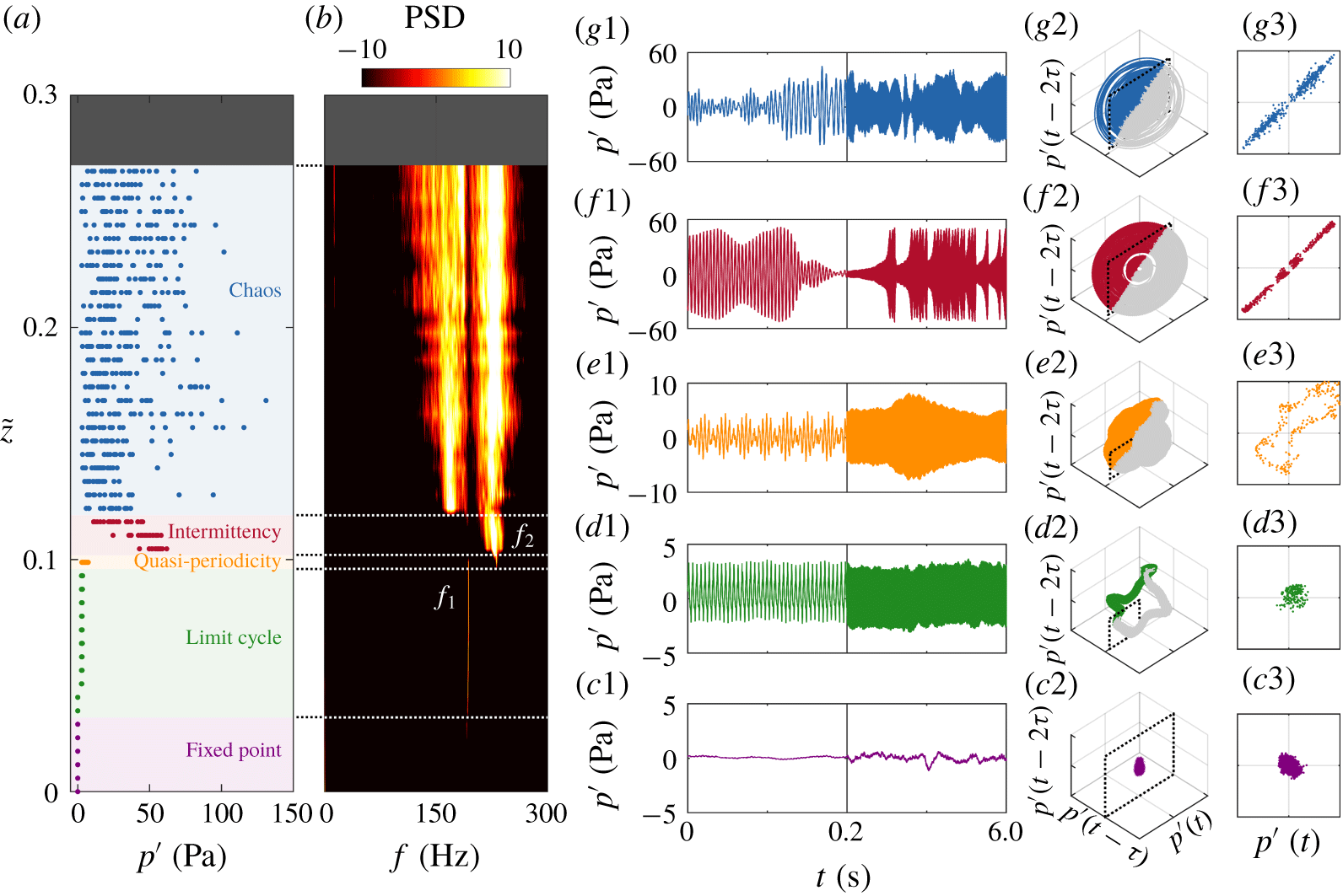
Figure 1. Overview of the system dynamics: (a) bifurcation diagram and (b) PSD of the combustor pressure fluctuations,  $p^{\prime }(t)$, as a function of the flame position, $\tilde{z}$. (c–g) Time traces (1), phase portraits (2) and Poincaré maps (3) for five dynamical states: (c) $\tilde{z}=0$, a fixed point; (d) $\tilde{z}=0.058$, a period-1 limit cycle; (e) $\tilde{z}=0.099$, 2-torus quasi-periodicity; (f) $\tilde{z}=0.116$, type-II intermittency; and (g) $\tilde{z}=0.122$, low-dimensional chaos. The flame blows off at $\tilde{z}\geqslant 0.267$.
(i) Fixed point: Initially ( $0\leqslant \tilde{z}<0.034$, purple markers/lines), the system is not thermoacoustically unstable, i.e. it is not self-excited. This is because the coupling between the HRR oscillations of the flame and the acoustic pressure oscillations of the combustor is not strong enough to overcome the dissipation in the system (Lieuwen & Yang Reference Lieuwen and Yang2005). This assessment is supported by the absence of high-amplitude features in the bifurcation diagram (figure 1a) and the time trace (figure 1c1), and by the absence of dominant peaks in the PSD (figure 1b). It is also supported by the presence of a ball-like structure at the origin of the phase portrait (figure 1c2), which leads to a single cluster of trajectory intercepts in the two-sided Poincaré map (figure 1c3). If the system were free of noise, its time trace would be perfectly steady, and its phase trajectory would converge to a discrete point at the origin. These observations indicate that the system is residing on a fixed-point attractor perturbed by low levels of noise.
(ii) Limit cycle: At higher flame positions (
$0.034\leqslant \tilde{z}<0.099$, green markers/lines), the system becomes thermoacoustically unstable (i.e. self-excited), having transitioned from a fixed point to a limit cycle via a Hopf bifurcation. This bifurcation is supercritical because the rise in the amplitude of $p^{\prime }(t)$ above the Hopf point ($\tilde{z}=0.034$), which marks the onset of thermoacoustic instability, is gradual rather than abrupt (figure 1a). The limit cycle produces a sharp peak at $f_{1}\approx 191~\text{Hz}$ in the PSD (figure 1b), near-sinusoidal oscillations in the time trace (figure 1d1), and a closed periodic orbit in the phase portrait (figure 1d2). The corresponding one-sided Poincaré map (figure 1d3) shows a single cluster of trajectory intercepts, indicating that the limit cycle is of period 1.(iii) Quasi-periodicity: At slightly higher flame positions (
$0.099\leqslant \tilde{z}<0.105$, orange markers/lines), the system remains thermoacoustically unstable, but admits a second self-excited natural mode. This can be seen in the PSD (figure 1b), where a new peak emerges at $f_{2}\approx 231~\text{Hz}$ alongside the peak at $f_{1}\approx 191~\text{Hz}$ from the original limit cycle. It can also be seen in the time trace (figure 1e1), which shows beating modulations characteristic of a self-excited oscillator with multiple modes (Li & Juniper Reference Li and Juniper2013a,Reference Li and Juniperb). Because the two modes ($f_{1}$ and $f_{2}$) are not commensurate (i.e. their winding number is not rational), the trajectory in the phase portrait is not closed (figure 1e2), but spirals non-repeatedly on the surface of a stable ergodic two-dimensional quasi-periodic attractor (2-torus), as evidenced by a closed ring in the one-sided Poincaré map (figure 1e3). These observations indicate that the system has transitioned from a period-1 limit cycle to an ergodic 2-torus quasi-periodic attractor via a Neimark–Sacker bifurcation.(iv) Intermittency: At even higher flame positions (
$0.105\leqslant \tilde{z}<0.122$, red markers/lines), the system exhibits intermittency. This is evidenced by the data points in the bifurcation diagram becoming more scattered as the system alternates between two different states (figure 1a): quasi-periodicity and chaos. This can be seen more clearly in the time trace (figure 1f1), where bursts of high-amplitude chaos appear intermittently over a background of medium-amplitude quasi-periodicity. Meanwhile, the second natural mode ($f_{2}$) strengthens relative to the first natural mode ($f_{1}$), dominating the PSD with a broad peak at $f_{2}$ (figure 1b). In phase space (figures 1f2 and 1f3), the system alternates between two different attractors: a 2-torus at the core and a strange attractor around it. If the phase trajectory is initially near the 2-torus (inner orbit), it remains there for some time and then bursts out to the strange attractor (outer orbit), before being re-injected to the 2-torus. This bursting and re-injection of the phase trajectory repeats intermittently, with the bursts of chaos lengthening in time as the bifurcation parameter ($\tilde{z}$) increases. The details of this intermittent state will be examined in § 3.2.(v) Chaos: At the highest flame positions (
$0.122\leqslant \tilde{z}<0.267$, blue markers/lines), the system becomes chaotic: the alternating epochs of quasi-periodicity and chaos observed during intermittency are replaced by a continuous regime of high-amplitude chaos (figure 1g1). This causes the data points in the bifurcation diagram to become even more scattered (figure 1a). In the PSD (figure 1b), the original natural mode ($f_{1}$) strengthens to match the second natural mode ($f_{2}$), with both modes being relatively broadband, a defining feature of chaos (Hilborn Reference Hilborn2000). Both the phase portrait (figure 1g2) and the Poincaré map (figure 1g3) show complex non-repeating fractal structures, which suggests the presence of a strange attractor associated with chaos. In § 3.3, we will verify the strange chaotic nature of this state using additional tools from dynamical systems theory. It is worth mentioning that chaotic thermoacoustic oscillations can arise from two distinct physical mechanisms (Huhn & Magri Reference Huhn and Magri2020): (a) the nonlinear HRR response of a flame to incident acoustic perturbations, and (b) turbulence-induced modulation of the HRR dynamics via the hydrodynamic field. The first mechanism is likely to be dominant in our laminar combustor, as previous numerical simulations have shown that chaotic thermoacoustic oscillations can be produced by the nonlinear saturation of laminar flame models, without the action of turbulent hydrodynamics (Kashinath et al. Reference Kashinath, Waugh and Juniper2014; Waugh, Kashinath & Juniper Reference Waugh, Kashinath and Juniper2014; Orchini, Illingworth & Juniper Reference Orchini, Illingworth and Juniper2015).


3.2 Analysis of intermittency
We analyse the intermittent state in more detail to better understand the route to chaos. We use a longer sampling time of 40 s to capture a sufficient number of alternation events for statistical convergence. Figures 2(a) and 2(b) show a 6 s window of the normalized pressure fluctuation signal (  $\tilde{p}^{\prime }\equiv p^{\prime }/|p^{\prime }|_{max}$) and its short-time PSD, respectively. Intermittent bursts of high-amplitude chaos can be seen amidst a background of medium-amplitude quasi-periodicity. The PSD of the chaotic bursts is characterized by a broad peak at $f_{2}$, whereas that of the quasi-periodic epochs is characterized by two relatively sharp peaks at $f_{1}$ and $f_{2}$, consistent with the phase trajectory evolving on an ergodic 2-torus.
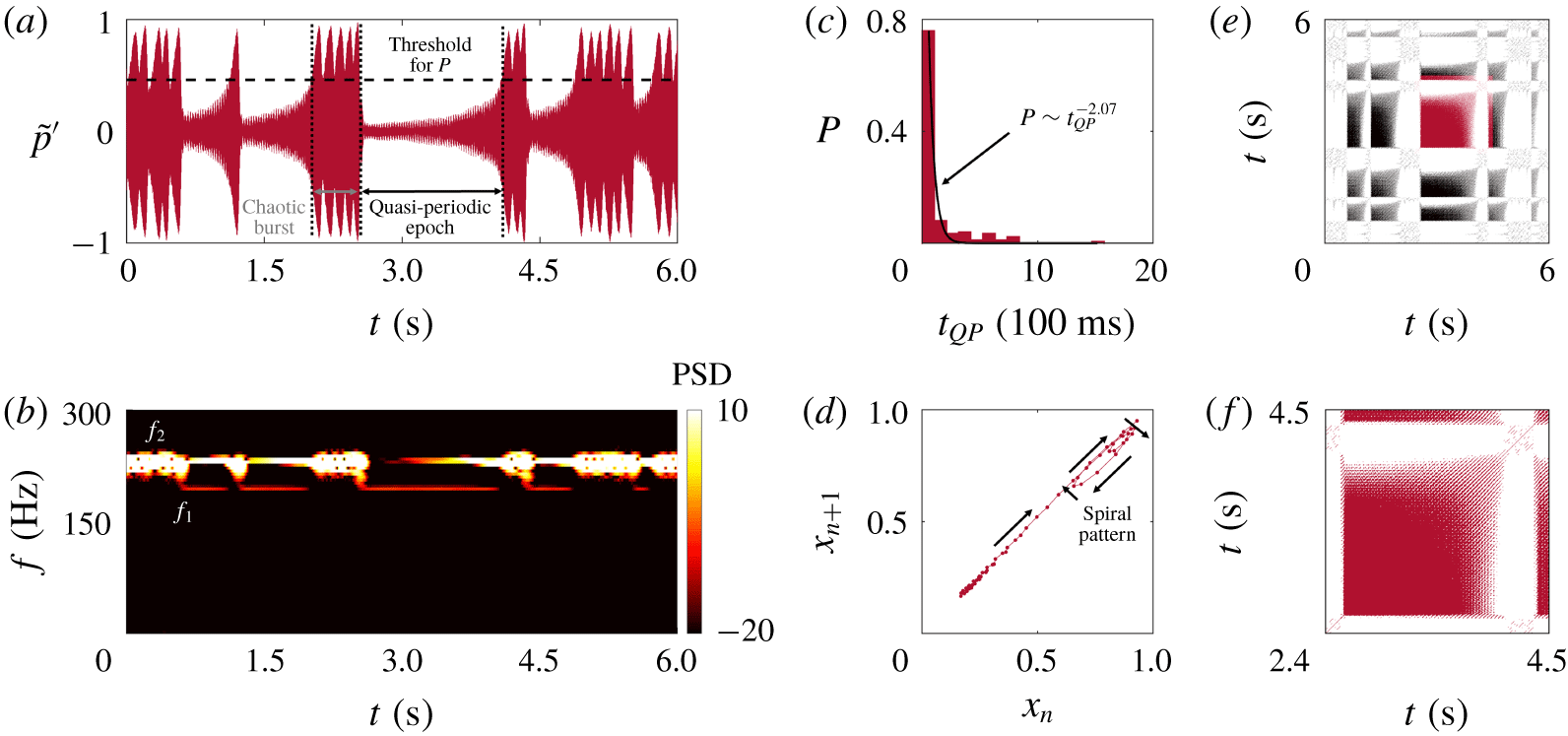
Figure 2. Evidence of type-II intermittency ( $\tilde{z}=0.116$): (a) a time trace of $p^{\prime }(t)$ showing bursts of high-amplitude chaos amidst a background of medium-amplitude quasi-periodicity; (b) the short-time PSD, (c) the probability distribution of the quasi-periodic epoch durations, (d) the first return map, (e) the recurrence plot (RP), and (f) a magnified view of the RP showing a kite-like structure.
Next we quantify the intermittent dynamics using three proven techniques. First, we compute the probability distribution of the duration of the quasi-periodic epochs ( $t_{QP}$) using the method of Hammer et al. (Reference Hammer, Platt, Hammel, Heagy and Lee1994). This involves setting an amplitude threshold in the time trace ( $\tilde{p}^{\prime }=0.5$; see the horizontal dashed line in figure 2a) and measuring the duration for which $\tilde{p}^{\prime }$ is below this threshold. These $t_{QP}$ values are then binned to create a histogram of the quasi-periodic durations $P$, as shown in figure 2(c). We find that $P$ exhibits a power-law decay with an exponent of -2.07 (95 % confidence) at small $t_{QP}$, followed by an exponential tail at large $t_{QP}$. This behaviour indicates the presence of type-II intermittency, for which theory based on random re-injections predicts an initial power-law exponent of -2 (Schuster & Just Reference Schuster and Just2006). By comparison, type-I intermittency is predicted to show a power-law decay with an exponent of -1/2 at small $t_{QP}$ followed by an increase at large $t_{QP}$, while type-III intermittency is predicted to show a power-law decay with an exponent of -3/2 at small $t_{QP}$ (Schuster & Just Reference Schuster and Just2006).
Second, we examine the first return map (figure 2d), where a vector of successive local maxima within the quasi-periodic epochs ( $x_{n}$) is plotted against a time-delayed version of itself ( $x_{n+1}$). We find that the data points cluster on the main diagonal, moving from the bottom left to the top right, before forming a spiral pattern characteristic of type-II intermittency (Sacher, Elsässer & Göbel Reference Sacher, Elsässer and Göbel1989). If this were type-I intermittency, the data points would cluster in a narrow channel off the main diagonal (Pomeau & Manneville Reference Pomeau and Manneville1980). If this were type-III intermittency, the data points would form a $\tan (x)$-like structure across the main diagonal (Schuster & Just Reference Schuster and Just2006). The presence of a spiral pattern in the first return map is thus further evidence of type-II intermittency (Sacher et al. Reference Sacher, Elsässer and Göbel1989).
Third, we examine the recurrence plot (RP). Introduced by Eckmann, Kamphorst & Ruelle (Reference Eckmann, Kamphorst and Ruelle1987), RPs have been used throughout science and engineering to uncover hidden patterns in time-series data, including to distinguish between different types of intermittency (Klimaszewska & Żebrowski Reference Klimaszewska and Żebrowski2009). Figures 2(e) and 2(f) show the RP for our system and its magnified view (highlighted in red), respectively. These figures are generated using the algorithm of Klimaszewska & Żebrowski (Reference Klimaszewska and Żebrowski2009), with an embedding dimension of  $d=10$, a time delay of $\unicode[STIX]{x1D70F}=2~\text{ms}$ and a recurrence threshold of 10 % of the largest attractor dimension. During bursts of high-amplitude chaos, the RP is sparsely populated (white regions), indicating little to no recurrence of the phase trajectory. As the system switches to an epoch of quasi-periodicity, a densely filled square with a stretched top-right corner emerges (figure 2f). In nonlinear dynamics, such a square is known as a kite-like structure and is a signature feature of type-II intermittency (Klimaszewska & Żebrowski Reference Klimaszewska and Żebrowski2009). Similar kite-like structures have previously been observed in both laminar (Kabiraj & Sujith Reference Kabiraj and Sujith2012) and turbulent (Pawar et al. Reference Pawar, Vishnu, Vadivukkarasan, Panchagnula and Sujith2016; Unni & Sujith Reference Unni and Sujith2017) combustors with type-II intermittency.
In summary, by examining (i) the probability distribution of the quasi-periodic epoch durations, (ii) the first return map and (iii) the RP, we have shown that the intermittency observed en route to chaos is of type II from the Pomeau & Manneville (Reference Pomeau and Manneville1980) scenario.
3.3 Analysis of chaos
As § 3.1 has shown, analysis of the  $p^{\prime }(t)$ signal in the time, frequency and phase domains suggests the existence of chaos after intermittency. To verify the existence of chaos and to analyse its properties, we use four proven tools from dynamical systems theory. We apply these tools to both a chaotic state and a periodic state, the latter for comparison purposes.
First, we apply the permutation spectrum test proposed by Kulp & Zunino (Reference Kulp and Zunino2014), using an embedding dimension of  $d=4$ and a time delay of $\unicode[STIX]{x1D70F}=1.2~\text{ms}$, for 20 different subsets of the $p^{\prime }(t)$ signal. For the periodic state (figures 3a1 and 3b1), the permutation spectra from the different subsets overlap reasonably well, with their standard deviation falling to zero ( $\unicode[STIX]{x1D701}\approx 0$) at many ordinal patterns, consistent with the limit-cycle nature of this state (Kulp & Zunino Reference Kulp and Zunino2014). For the chaotic state (figures 3a2 and 3b2), the permutation spectra are more scattered, resulting in $\unicode[STIX]{x1D701}\approx 0$ at only three ordinal patterns: 3, 16 and 22 (see inset of figure 3b2). Crucially, these ordinal patterns form forbidden patterns with symbolic sequences of 1-3-2-4, 3-2-4-1 and 4-2-3-1, respectively. Such forbidden patterns are characteristic of deterministic chaos (Kulp & Zunino Reference Kulp and Zunino2014).
Second, we compute the correlation dimension ( $\overline{D_{c}}$) using the algorithm of Grassberger & Procaccia (Reference Grassberger and Procaccia1983). This provides an estimate of the number of active degrees of freedom in the system, thus quantifying the topological self-similarity of the attractors. Figure 3(c) shows the local slope of the correlation sum ( $D_{c}\equiv \unicode[STIX]{x2202}\log C_{N}/\unicode[STIX]{x2202}\log R$) as a function of the normalized hypersphere radius ( $R/R_{max}$) for three embedding dimensions ( $d=10$, 12 and 14). For the periodic state (figure 3c1), $D_{c}$ converges to an average of $\overline{D_{c}}\approx 1.0$ within the self-similar Euclidean scaling range ( $10^{-1}\leqslant R/R_{max}\leqslant 10^{-0.4}$), indicating limit-cycle dynamics. For the chaotic state (figure 3c2), $D_{c}$ converges to an average of $\overline{D_{c}}\approx 3.6$ within $10^{-1.8}\leqslant R/R_{max}\leqslant 10^{-1.2}$. Such a non-integer value of $\overline{D_{c}}$ indicates that the attractor is strange (Hilborn Reference Hilborn2000). Moreover, the relatively low value of $\overline{D_{c}}$ indicates that the chaotic dynamics is low-dimensional (Hilborn Reference Hilborn2000). Collectively, these findings are consistent with our earlier observations of broadband components in the PSD (figure 1b) and irregular geometrical structures in phase space (figure 1g3).
Third, we use the 0–1 test from Gottwald & Melbourne (Reference Gottwald and Melbourne2004) to distinguish between non-chaotic and chaotic dynamics. This test has been successfully used to detect determinism in combustion noise (Nair et al. Reference Nair, Thampi, Karuppusamy, Gopalan and Sujith2013) and self-excited thermoacoustic oscillations (Vishnu et al. Reference Vishnu, Sujith and Aghalayam2015). We find that the translation components ( $m_{c},n_{c}$) undergo circular motion for the limit-cycle attractor (figure 3d1) but Brownian-like motion for the strange attractor (figure 3d2), indicating chaos in the latter. Although not shown here for brevity, the $K$ value is close to zero for the limit-cycle attractor, but is around one for the strange attractor, further confirming the presence of chaos in the latter.
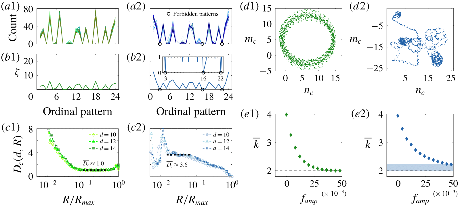
Figure 3. Evidence of low-dimensional chaos: (a) permutation spectra and (b) their standard deviation, (c) the local slope of the correlation sum as a function of the normalized hypersphere radius, (d) translation components from the 0–1 test, and (e) the mean degree of the filtered-horizontal visibility graph (f-HVG) as a function of the noise-filter amplitude. Data are shown for (green) a limit-cycle attractor at  $\tilde{z}=0.058$, and (blue) a strange attractor at $\tilde{z}=0.122$.
Fourth, we use the filtered-horizontal visibility graph (f-HVG) from Nuñez et al. (Reference Nuñez, Lacasa, Valero, Gómez and Luque2012) to distinguish between periodic and chaotic dynamics. Visibility graphs were introduced in thermoacoustics by Murugesan & Sujith (Reference Murugesan and Sujith2015). The f-HVG works by converting a time series into network structures via graph theory. For the limit-cycle attractor (figure 3e1), we find that the mean degree  $\overline{k}$ converges to exactly 2 as the noise-filter amplitude $f_{amp}$ increases, indicating a temporal period of $T=1$, which is consistent with our earlier assessment (§ 3.1) that this limit cycle is of period 1. For the strange attractor (figure 3e2), we find that $\overline{k}$ has not yet converged to 2, despite the noise-filter amplitude being at a value ( $f_{amp}=0.05$) high enough to induce $\overline{k}=2$ in the limit-cycle attractor. This absence of convergence in $\overline{k}$ is consistent with chaos (Nuñez et al. Reference Nuñez, Lacasa, Valero, Gómez and Luque2012).
In summary, by considering (i) the permutation spectrum test, (ii) the correlation dimension, (iii) the 0–1 test and (iv) the f-HVG, we have established the existence of a self-excited state of low-dimensional chaos on a strange attractor. When combined with the evidence from § 3.2, this confirms a transition to chaos via type-II intermittency.
4 Conclusions
In this experimental study, we have presented evidence of the intermittency route to chaos in the self-excited regime of a prototypical laminar thermoacoustic system. On increasing the bifurcation parameter  $\tilde{z}$, we find five different dynamical states: a fixed point → a period-1 limit cycle → 2-torus quasi-periodicity → type-II intermittency from the Pomeau & Manneville (Reference Pomeau and Manneville1980) scenario → low-dimensional chaos. The intermittent state is characterized by bursts of high-amplitude chaos appearing intermittently over a background of medium-amplitude quasi-periodicity. The type-II nature of this state is confirmed by: (i) a power-law decay in the probability distribution of the quasi-periodic epoch durations, with an exponent close to the theoretically predicted value of -2 at small $t_{QP}$; (ii) a spiralling trajectory in the first return map; and (iii) kite-like structures in the RP. The presence of low-dimensional chaos is confirmed by: (i) forbidden patterns in the permutation spectrum test; (ii) a non-integer correlation dimension of $\overline{D_{c}}\approx 3.6$; (iii) Brownian-like motion in the translation components of the 0–1 test, along with $K\approx 1$; and (iv) a non-convergent mean degree in the f-HVG. Together, these indicators provide compelling evidence of a transition to low-dimensional chaos via type-II intermittency.
Establishing the intermittency route to chaos is important because it is the last of the three classic routes to chaos to be discovered in self-excited thermoacoustic systems, the other two being the period-doubling route and the RTN route. This study thus strengthens the universality of how strange attractors arise in self-excited thermoacoustic systems, setting the stage for the application of generic suppression methods based on chaos control (Schöll & Schuster Reference Schöll and Schuster2008; Huhn & Magri Reference Huhn and Magri2020).
As a final remark, it is worth recalling that, although intermittency involving chaos has previously been observed in the low-amplitude (combustion noise) regime of thermoacoustic systems (Nair et al. Reference Nair, Thampi, Karuppusamy, Gopalan and Sujith2013, Reference Nair, Thampi and Sujith2014), it has not, until now, been observed in the high-amplitude (self-excited) regime. This is an important distinction because, in practical combustors, the high-amplitude pressure oscillations arising after the onset of thermoacoustic instability have a greater potential to inflict mechanical damage and impair flame stability than the low-amplitude fluctuations associated with combustion noise (Lieuwen & Yang Reference Lieuwen and Yang2005). Crucially, if those high-amplitude oscillations happen to be chaotic, with their kinetic energy distributed over a broad range of frequencies, then they will have a greater potential to couple with the natural structural modes of the combustor hardware, producing more destructive fatigue loads via resonance (Suresh Reference Suresh1998). Here we have shown that chaos can arise via intermittency in the self-excited regime, after the onset of thermoacoustic instability. This implies that many of the early-warning indicators used to forecast the onset of limit-cycle oscillations based on a loss of chaos in the combustion-noise regime (Gotoda et al. Reference Gotoda, Shinoda, Kobayashi, Okuno and Tachibana2014; Nair & Sujith Reference Nair and Sujith2014; Juniper & Sujith Reference Juniper and Sujith2018) may be repurposed to forecast the onset of chaotic oscillations in the self-excited regime. The extent to which this can be achieved, particularly in turbulent combustors, remains to be determined.
Acknowledgements
This work was funded by the Research Grants Council of Hong Kong (project nos 16235716, 26202815 and 16210418). V.G. was supported by the National Natural Science Foundation of China (grant nos 11672123 and 91752201), the Department of Science and Technology of Guangdong Province (grant no. 2019B21203001), and the Shenzhen Science and Technology Innovation Committee (grant nos JCYJ20170412151759222 and KQTD20180411143441009).
Declaration of interests
The authors report no conflict of interest.


 Open access