


1. Introduction
Emulsions composed of two immiscible and incompressible liquids are omnipresent in many industrial fields such as food processing (McClements Reference McClements2005), pharmaceutics (Nielloud & Marti-Mestres Reference Nielloud and Marti-Mestres2000) and chemical engineering (Ahmad et al. Reference Ahmad, Kusumastuti, Derek and Ooi2011). Because of their practical importance, such two-liquid emulsions have been studied extensively. However, the physical mechanisms behind their dynamics are not well understood, and many open questions remain.
One of the most important features of emulsions is their interface dynamics, i.e. deformation, coalescence and breakup. Since the two liquids are immiscible, they are completely separated by the deformable interface. Through momentum exchange, the deformation affects the neighbouring velocity field, and vice versa. When the external hydrodynamic load is strong enough, the interface is largely elongated and eventually breaks up into multiple fragments. Hinze (Reference Hinze1955) provided a simple analysis of such droplet breakup in homogeneous isotropic turbulence. His theory well described the size of droplets in many systems (Garrett, Li & Farmer Reference Garrett, Li and Farmer2000; Rosti et al. Reference Rosti, Ge, Jain, Dodd and Brandt2019b). However, since his theory assumes that the volume fraction is so low that the interactions between droplets are negligible, it breaks down when two interfaces get so close to each other that van der Waals forces come into play (Falzone et al. Reference Falzone, Buffo, Vanni and Marchisio2018) and coalescence becomes more likely. Such effects are non-negligible for high volume fraction cases.
In order to analyse the effects of droplet coalescence and fragmentation in emulsions whose volume fractions are above the dilute regime and the theory by Hinze is not applicable, direct numerical simulations provide some crucial insights. How the coalescence plays a role on the suspension rheology was studied numerically by Rosti, De Vita & Brandt (Reference Rosti, De Vita and Brandt2019a) and De Vita et al. (Reference De Vita, Rosti, Caserta and Brandt2019) for the Stokes regime. Rosti et al. (Reference Rosti, De Vita and Brandt2019a) focused on the rheological effect of the surface deformability and the volume fraction of the secondary phase in plane Couette flows by means of interface-resolved direct numerical simulations that could handle topological changes. De Vita et al. (Reference De Vita, Rosti, Caserta and Brandt2019) extended this work by introducing a short-range repulsive force to suppress the coalescence, focusing on how the coalescence affected the effective viscosity. When the repulsive force was added and the coalescence was less likely, the effective viscosity as a function of the volume fraction showed a monotonic increase, which was the same trend observed for rigid particle suspensions (Guazzelli, É., Pouliquen Reference Guazzelli, É., Pouliquen2018) and deformable particles (Rosti & Brandt Reference Rosti and Brandt2018). When the repellent force was absent and the coalescence became dominant, on the other hand, the effective viscosity as a function of the total volume fraction showed a non-monotonic curve with a maximum at  $\varphi \approx 20\,\%$. They concluded that this non-monotonic trend was caused by a competing effect between the increase in the surface area trying to increase the effective viscosity, and the coalescence trying to reduce it. These findings highlight that the rheology of two-liquid emulsions can be affected largely by the coalescing events of the interface. Also, two-liquid emulsions in a turbulent regime, in which inertial and interfacial effects dominate viscous effects, have been a subject of interest in various numerical studies. Such studies focus mainly on droplet size distributions (Mukherjee et al. Reference Mukherjee, Safdari, Shardt, Kenjereš and Van den Akker2019; Soligo, Roccon & Soldati Reference Soligo, Roccon and Soldati2019; Crialesi-Esposito et al. Reference Crialesi-Esposito, Rosti, Chibbaro and Brandt2022) or global system responses, such as the skin friction coefficient (Roccon, Zonta & Soldati Reference Roccon, Zonta and Soldati2019, Reference Roccon, Zonta and Soldati2021) or the heat flux (Liu et al. Reference Liu, Chong, Ng, Verzicco and Lohse2022).
In this work, in order to focus on the rheological behaviours of two-liquid flows, we employ a Taylor–Couette (TC) system as a model set-up, which is the flow between two coaxial and independently rotating cylinders. Not only being used practically as a mixing tool in the field of chemical engineering (Schrimpf et al. Reference Schrimpf, Esteban, Warmeling, Färber, Behr and Vorholt2021), the TC system is one of the most paradigmatic in fluid mechanics (Fardin, Perge & Taberlet Reference Fardin, Perge and Taberlet2014; Grossmann, Lohse & Sun Reference Grossmann, Lohse and Sun2016) because of its closed and well-controlled geometry. One of the most pronounced features of TC flows is the typical secondary flow structure that is characterised by the azimuthal vortical structures, namely Taylor rolls. In fact, it is observed that the interaction between bubbles, Taylor rolls and turbulence produces substantial effects on the skin friction of the system, which is known as bubbly drag reduction (Murai Reference Murai2014; Lohse Reference Lohse2018). In order to reveal the mechanism of this drag reduction induced by bubbles, TC flows are used widely experimentally, from the relatively low Reynolds number regime up to  $5 \times 10^3$ (Murai, Oiwa & Takeda Reference Murai, Oiwa and Takeda2008; Murai et al. Reference Murai, Tasaka, Oishi and Takeda2018) to the extremely turbulent regime up to $2 \times 10^6$ (van den Berg et al. Reference van den Berg, Luther, Lathrop and Lohse2005, Reference van den Berg, van Gils, Lathrop and Lohse2007; van Gils et al. Reference van Gils, Narezo Guzman, Sun and Lohse2013). From a numerical point of view, among others, Sugiyama, Calzavarini & Lohse (Reference Sugiyama, Calzavarini and Lohse2008) and Spandan, Verzicco & Lohse (Reference Spandan, Verzicco and Lohse2018) analysed how the flow fields (e.g. torque response) were modified by adding bubbles in detail. Sugiyama et al. (Reference Sugiyama, Calzavarini and Lohse2008) focused on relatively low Reynolds numbers ( $Re \equiv r_i \omega _i d / \nu = 6 \times 10^2\unicode{x2013}2.5 \times 10^3$, from a stable Taylor vortex regime to a wavy vortex flow regime), where bubbles were shown to intervene in the formations of the Taylor rolls. For larger $Re$ in the turbulent regime ( $Re = 5 \times 10^3\unicode{x2013}2 \times 10^4$), Spandan et al. (Reference Spandan, Verzicco and Lohse2018) observed that the bubbles decrease the dissipation close to the wall. Although these two works considered different flow regimes, thus background mechanisms of the drag reduction are totally different, they revealed independently that bubbles can reduce the drag by modulating the secondary flow structures, highlighting the importance of the interactions between interfaces and flow fields.
How secondary flow structures and suspended objects interact with each other has been studied widely for rigid particle suspensions. Majji & Morris (Reference Majji and Morris2018) focused on the inertial migration of neutrally buoyant and finite-sized rigid particles experimentally by varying the Reynolds numbers for various flow regimes to find the equilibrium positions of the suspended particles. They revealed that the equilibrium positions were changed drastically for different flow regimes, starting from the centre of the channel (circular Couette flow regime), followed by circular regions in the  $r$–
$r$– $z$ plane (Taylor vortex flow regime), and eventually distributing uniformly (wavy vortex flow regime). Assen et al. (Reference Assen, Ng, Will, Stevens, Lohse and Verzicco2022) analysed numerically the motions of finite-sized elliptic objects in Taylor–Couette flows from the Taylor vortex flow regime to the turbulent regime. They observed that the behaviour of particles (e.g. rotations in the flow, equilibrium positions) is Reynolds-number-dependent, describing a large influence of the Taylor vortices on the motions of particles. Also, the effects of particles on flow fields, i.e. how the suspensions modulate the Taylor rolls, have been actively explored recently. Gillissen & Wilson (Reference Gillissen and Wilson2019) analysed theoretically how the stability of circular Couette flow was affected by additional finite-sized particles. They found that the interactions between neighbouring particles destabilised the flow field and thus made the transition to the Taylor vortex flow regime easier. Ramesh, Bharadwaj & Alam (Reference Ramesh, Bharadwaj and Alam2019) studied experimentally how the particles affected the critical Reynolds numbers at which the transition from one state to the other occurred. They observed that for suspensions whose volume fractions were larger than $5\,\%$, critical Reynolds numbers tended to be reduced, and moreover, multiple flow regimes could coexist by the presence of particles. Dash, Anantharaman & Poelma (Reference Dash, Anantharaman and Poelma2020) focused experimentally on the particulate TC flows for more strongly-driven conditions up to $Ta = O ( 10^7 )$. They observed azimuthally localised wavy structures, indicating that the particles enhanced the flow instability. These works highlighted the crucial effects of Taylor rolls on the behaviour of dispersed phases, and also the important roles played by the particles on the modulations of the flow fields.
Taylor–Couette systems have been adopted actively to investigate turbulent two-liquid flows (e.g. emulsions) experimentally (Farzad et al. Reference Farzad, Puttinger, Pirker and Schneiderbauer2018; Bakhuis et al. Reference Bakhuis, Ezeta, Bullee, Marin, Lohse, Sun and Huisman2021; Yi, Toschi & Sun Reference Yi, Toschi and Sun2021; Yi et al. Reference Yi, Wang, van Vuren, Lohse, Risso, Toschi and Sun2022), where interesting physical phenomena were revealed. Yi et al. (Reference Yi, Toschi and Sun2021) analysed oil droplets in ethanol–water mixtures by varying the total volume fraction  $\varphi$ up to $40\,\%$ and the Reynolds number up to $2.6 \times 10^4$ . When $\varphi$ is sufficiently low (e.g. $\varphi = 1\,\%$), they observed that the mean droplet size well followed the Hinze scaling (Hinze Reference Hinze1955) even in the TC geometry. Interestingly, they noticed that the effective viscosity of the emulsion decreased with increasing the inner cylinder rotation, i.e. showing a shear-thinning trend, and the reduction was more noticeable when the volume fraction is high. This work was followed by Yi et al. (Reference Yi, Wang, van Vuren, Lohse, Risso, Toschi and Sun2022) recently, where they reported how the rheological behaviour and the droplet size distributions differ from water-in-oil and oil-in-water emulsions for various volume fractions. They found that although the physical properties of water and oil were very similar to each other, the rheologies of water-in-oil and oil-in-water mixtures were totally different. They concluded that this asymmetry was caused by the impurity that was inevitable experimentally, and highlighted the importance of surface-active contaminants. A wider $\varphi$ range (the turbulent regime, $Re$ up to $2 \times 10^6$) was investigated experimentally by Bakhuis et al. (Reference Bakhuis, Ezeta, Bullee, Marin, Lohse, Sun and Huisman2021). Water–oil mixtures spanning the full $\varphi$ regime ( $\varphi = 0\,\%\unicode{x2013}100\,\%$) were considered. These authors reported catastrophic phase inversions (swapping of the carrier and dispersed phases) and the resulting sudden jumps in the effective viscosity. The causes of these physically interesting phenomena, however, were not completely understood, and several aspects need to be explained.
In this work, in order to gain deeper insight into the interplay between TC flows and deformable interfaces, we use direct numerical simulation. There are some prior numerical studies simulating the behaviour of two immiscible liquids in TC geometries (Nakase & Takeshita Reference Nakase and Takeshita2012; Verdin et al. Reference Verdin, Charton, Roussel and Maurel2016; Nakase, Matsuzawa & Takeshita Reference Nakase, Matsuzawa and Takeshita2018; Franken Reference Franken2020; Morenko Reference Morenko2021). However, compared to single-phase or particle-laden TC flows, quantitative discussions and physical insights on the two-liquid flows are still limited, and no high-fidelity numerical simulations have been reported, to the best of our knowledge. Here, we will discuss the basic dynamics of two-liquid flows in TC flow obtained by a high-performance direct numerical simulation tool ‘AFiD’ (van der Poel et al. Reference van der Poel, Ostilla-Mónico, Donners and Verzicco2015), which is based on a second-order-accurate finite-difference method (Verzicco & Orlandi Reference Verzicco and Orlandi1996) and has been used to study various turbulent TC flows (Ostilla-Mónico, Lohse & Verzicco Reference Ostilla-Mónico, Lohse and Verzicco2016; Spandan et al. Reference Spandan, Verzicco and Lohse2018; Zhu et al. Reference Zhu, Verschoof, Bakhuis, Huisman, Verzicco, Sun and Lohse2018; Assen et al. Reference Assen, Ng, Will, Stevens, Lohse and Verzicco2022). In order to describe the interfacial motions, the method is combined with a state-of-the-art volume-of-fluid method (Ii et al. Reference Ii, Sugiyama, Takeuchi, Takagi, Matsumoto and Xiao2012; Xie & Xiao Reference Xie and Xiao2017). Before analysing two-liquid flows in turbulent TC flows on which we will focus in future work, in this paper we limit our discussion to a relatively low  $Re$ regime (steady Taylor vortex regime). The questions that we aim to answer here are as follows. (i) How does the interface interact with the background velocity field (Taylor vortices)? (ii) How does the interface affect the global response of the system? In this work, we focus on these questions by varying two non-dimensional parameters: the Weber number $We$ and the phase volume fraction $\varphi$.
This paper is organised as follows. In § 2, we describe the problem set-up and present the governing equations. The flow structures are presented and discussed in § 3. The influence of the secondary phase on Taylor rolls is presented in § 4.1 and quantified using one-dimensional velocity spectra in § 4.2. Next, the global torque response is discussed in § 5, where we also explain the changes in the torque response with increasing  $\varphi$ by quantifying the individual contributions to the Nusselt number. Finally, in § 6, we summarise our key findings and provide an outlook for future work.
2. Problem set-up
2.1. Governing equations
We consider two immiscible and incompressible liquids confined between two coaxial cylinders whose radii are  $r_i$ (inner) and $r_o$ (outer), and the axial length is $L_z$. In this work, we fix the outer cylinder and let the inner one rotate with a constant angular velocity $\omega _i$. The two liquid phases are governed by the incompressibility constraint
 \begin{equation} \boldsymbol{\nabla} \boldsymbol{\cdot} \boldsymbol{u} = 0 \end{equation}
and the balance of momentum
 \begin{equation} \frac{\partial \boldsymbol{u}}{\partial t} + \boldsymbol{u} \boldsymbol{\cdot} \boldsymbol{\nabla} \boldsymbol{u} ={-}\frac{1}{\rho}\,\boldsymbol{\nabla} p + \nu\,\nabla^2 \boldsymbol{u} + \frac{1}{\rho}\,\boldsymbol{f}. \end{equation}
Here,  $\boldsymbol {u} = \boldsymbol {u} ( \boldsymbol {x}, t )$ and $p = p ( \boldsymbol {x}, t )$ denote the fluid velocity and the reduced pressure, respectively. Note that $\rho$ and $\nu$, which are the density and kinematic viscosity, respectively, have the same values for both liquids in this work, and thus take constant values. Also, $\boldsymbol {f} = \boldsymbol {f} ( \boldsymbol {x}, t )$ describes the interfacial contribution to the momentum balance. It is written as
 \begin{equation} \boldsymbol{f} = \sigma\,\kappa ( \boldsymbol{x}, t )\,\delta \boldsymbol{n} ( \boldsymbol{x}, t ), \end{equation}
where  $\sigma$, $\kappa$, $\delta$ and $\boldsymbol {n}$ are the surface tension coefficient, local curvature, Dirac delta function and local normal vector, respectively. In addition to those two equations, we consider an advection equation with respect to the indicator function $H$,
$H$,
 \begin{equation} \frac{\partial H}{\partial t} + \boldsymbol{u} \boldsymbol{\cdot} \boldsymbol{\nabla} H = 0, \end{equation}
to distinguish the two liquids. The indicator function  $H$ equals $0$ where the primary phase is, and $1$ if the region is occupied by the secondary phase. Equations (2.1) and (2.2) are solved by a second-order-accurate finite-difference scheme in cylindrical coordinates (Verzicco & Orlandi Reference Verzicco and Orlandi1996; van der Poel et al. Reference van der Poel, Ostilla-Mónico, Donners and Verzicco2015).
2.2. Volume-of-fluid method
In this subsection, we describe briefly the method employed to integrate (2.4) and to solve the interfacial contribution  $\boldsymbol{f}$ in (2.2). Here, $\boldsymbol{f}$, which is described mathematically as in (2.3), is modelled with the continuum-surface-force approach (Brackbill, Kothe & Zemach Reference Brackbill, Kothe and Zemach1992; Ii et al. Reference Ii, Sugiyama, Takeuchi, Takagi, Matsumoto and Xiao2012)
 \begin{equation} \boldsymbol{f} \approx \sigma \kappa\,\boldsymbol{\nabla} \phi, \end{equation}
where  $\phi$ is the so-called ‘volume-of-fluid’ defined as the volume average of $H$ in a control volume $\mathcal {V}$. By averaging (2.4) in $\mathcal {V}$, we obtain the advection equation with respect to $\phi$ as
 \begin{equation} \frac{\partial \phi}{\partial t} ={-}\int_{\partial \mathcal{V}} \boldsymbol{u} H \boldsymbol{\cdot} \boldsymbol{n} \,\mathrm{d}\mathcal{S} + \phi\,\boldsymbol{\nabla} \boldsymbol{\cdot} \boldsymbol{u}, \end{equation}
where  $\int _{\partial \mathcal {V}} (\cdot )\,\mathrm {d}\mathcal {S}$ denotes the surface integral on the control volume. To compute this surface integral, we extended the THINC/QQ scheme (Xie & Xiao Reference Xie and Xiao2017) to cylindrical coordinates (see Appendix B for details).
2.3. Flow parameters
For the TC set-up, we set the curvature as  $\eta \equiv r_i / r_o = 0.714$ and the aspect ratio as $\varGamma \equiv L_z / d = 2{\rm \pi}$, where $d \equiv r_o - r_i$ is the gap width. No-slip and impermeable boundary conditions are imposed in the radial direction, while periodicity is imposed in the axial direction. As shown in figure 1, we employ the full azimuthal cylinder domain because large fluid structures composed of the secondary phase can exist. The cylinder is discretised by $( 128, 1920, 720 )$ grid points in the radial, azimuthal and axial directions, respectively. The clipped-Chebyshev clustering is adopted in the radial direction to resolve boundary layers near the walls, while grid points are uniformly spaced in the other homogeneous directions. Details of the spatial resolution effects and code validations and verifications are described in §§ C.2 and C.5.

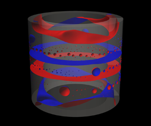
Figure 1. Instantaneous interface snapshots for different total volume fractions  $\varphi$ and $We$. The iso-surface $\phi = 0.5$ is shown, where the regions surrounded by the bluish and reddish surfaces are filled by the primary ( $\phi < 0.5$) and secondary ( $\phi > 0.5$) phases, respectively. Two co-axial transparent cylinders denote the boundaries of the geometry. Weber numbers (a–e) $We = 400$ (high $We$), and (f–j) $We = 40$ (low $We$). The volume fraction $\varphi$ is increased from left to right, from $10\,\%$ to $50\,\%$.
We fix the Reynolds number  $Re \equiv r_i \omega _i d / \nu = 960$, which is in the steady Taylor vortex regime (Grossmann et al. Reference Grossmann, Lohse and Sun2016). The two control parameters characterising the secondary phase are its total volume fraction $\varphi$ and the (system) Weber number $We \equiv \rho r_i^2 \omega _i^2 d / \sigma$. We consider ten different total volume fractions $\varphi = 5\,\%, 10\,\%, 15\,\%, \ldots, 50\,\%$, and two system Weber numbers $We = 40, 400$. In addition, we impose the Neumann boundary condition with respect to $\phi$, resulting in a $90^\circ$ contact angle for the secondary phase.
It should be noted that as discussed in the Introduction, there are several parameters that are expected to play crucial roles in the fluid dynamics but are missing in this work. We consider that they are the density ratio between two fluids, and the Reynolds number, among others. When the density ratio between two liquids is not unity, one would expect that the phase having smaller density tends to migrate to the inner cylinder because of the centrifugal force, affecting the phase distributions. When the Reynolds number is varied, interactions between interfacial structures and different turbulent intensities could pose many interesting phenomena. However, even for a fixed and relatively small Reynolds number with unitary density ratio, interplay between flow fields (in particular Taylor rolls) and the surface is rarely studied and is worth being examined. Although this is the reason why we do not consider these parameters in this work, they are to be analysed in the near future.
First, we simulate a single-phase case to initialise the velocity field. Once we obtain a well-developed flow having two pairs of Taylor rolls, the simulation is restarted after some spherical droplets with diameter  $0.08 d$ are positioned randomly. The droplets coalesce (because of the contact with different droplets) and break up (because of shear) continuously, and eventually adapt to the flow field. All the statistics presented are collected for at least $100$ time units after the statistically steady state is reached, which is determined by monitoring the time evolution of the Nusselt number (whose variation is within $\approx 4\,\%$) and the interface area (see § C.5).
3. Flow visualisations
We start our discussions with a qualitative description of the flow features. In figure 1, we show the instantaneous interface structures for  $\varphi$ ranging from $10\,\%$ to $50\,\%$ for both $We$ values, where figures 1(a–e) and 1(f–j) show high $We = 400$ and low $We = 40$, respectively. Note that we shift each flow field in the $z$ direction for visualisation purposes, so that the plume-ejecting region (axial location $z$, where $\langle u_r \rangle _{\theta,t}$ takes the maximum) appears in the middle of each snapshot. This is justified since we impose periodic boundary condition in the axial direction. We perform the same treatment for figures 3 and 4.
For high  $We = 400$ and at the lowest volume fraction ( $\varphi = 10\,\%$), we observe many small spherical droplets. We also observe that some droplets are connected by ligaments or one is partially elongated, which corresponds to coalescence and breaking up, respectively. The balance of these two processes results in a constant surface area of the interface (see § C.5). The mean droplet size increases with increasing $\varphi$, which is simply because coalescence becomes more likely. Eventually, toroidal structures form at higher volume fractions ( $\varphi = 40\,\%, 50\,\%$). At $50\,\%$, the appearance is totally different, in which the phase touching on the walls is changed from the primary phase ( $\phi < 0.5$) to the secondary phase ( $\phi > 0.5$). The occurrence of the phase inversion here is reasonable since each phase has the same volume fraction.
For the lower  $We = 40$ and at low volume fraction $\varphi = 10\,\%$, the interfacial structures are noticeably different. In particular, small droplets rarely exist, and rather, the dispersed phase organises in larger and less spherical patches as compared to the high $We$ case. These large droplets are stretched in the azimuthal direction and extend partially through the gap. As $\varphi$ is increased, annuli-like large structures spanning the azimuthal direction start to appear, which are dominant for $\varphi = 20\,\%$ and $30\,\%$. Further increase in $\varphi$ results in the formation of some ring-like interfaces ( $\varphi = 40\,\%,50\,\%$), implying that the two liquids are separated in the axial direction and are layered.
For all volume fractions for lower  $We = 40$ (figures 1f–j), we notice that small-scale droplets are distributed along the azimuthal direction on the outer cylinder walls, which originate from the droplet touching the walls initially. While these structures on the walls are affected by the Taylor rolls and transported in the axial direction, they can stay on the walls thanks to the strong surface tension, and create visible structures where the plumes are ejected. For higher $We = 400$, on the other hand, these droplets touching on the walls are eventually swept away by the Taylor rolls owing to the weak surface tension, which does not form these structures on the walls.
Since the two set-ups exhibit rich morphological structures, it is useful to quantify and distinguish the morphological characteristics. To do so, we compute the probability density function (p.d.f.) of the surface curvature here, which was studied in the literature to characterise the surface deformation in turbulence (Roccon et al. Reference Roccon, De Paoli, Zonta and Soldati2017; Canu et al. Reference Canu, Puggelli, Essadki, Duret, Menard, Massot, Reveillon and Demoulin2018). We compute the mean curvature  $\kappa$ from the snapshots (figure 1), which is plotted in figure 2 after being normalised by the radius of the inner cylinder $r_i$. When two $We$ cases are compared, we notice that higher $We$ cases (figure 2a) have smaller kurtosis than lower $We$ cases (figure 2b). This shows that higher $We$ cases tend to create droplets having a variety of sizes associated with the breaking up and coalescing phenomena, whilst lower $We$ cases prefer to form stable structures with less varied sizes. For lower $We$ cases, up to $\varphi = 30\,\%$, we observe that the maximum probability exists in the positive region ( $r_i \kappa > 0$), which indicates that the phase characterised by $\phi = 1$ (i.e. the phase contained by the reddish surface in figure 1) tends to be suspended in the other phase $\phi = 0$ (the phase contained by the bluish surface in figure 1). As the volume fraction is increased ( $\varphi = 40\,\%, 50\,\%$), on the other hand, the profiles are nearly symmetric with respect to the centre $r_i \kappa = 0$, which well quantifies the planner structures that separate two phases in the axial direction (see figure 1i,j). For higher $We$ cases at the lowest volume fraction $\varphi = 10\,\%$, being similar to the lower $We$ cases, the profile is clearly right-shifted, indicating that many small droplets composed of $\phi = 1$ are suspended in the other phase $\phi = 0$. The centre of the profiles approaches $r_i \kappa = 0$ rapidly as the volume fraction is increased, which is because coalescing phenomena are more likely, and small droplets are less probable. Finally, an almost perfectly symmetric profile is observed at the highest volume fraction $50\,\%$. Note that the origin of this symmetry is not the planner surface, but the phase inversion observed in figure 1(j), i.e. it is no longer possible to tell the difference between suspended and carrier phases.

Figure 2. Probability density functions (p.d.f.s) of the mean curvature  $\kappa$ normalised by the radius of the inner cylinder $r_i$, for (a) high $We = 400$, and (b) low $We = 40$. Different colours are used to distinguish different volume fractions.
To quantify the distribution of each phase, we plot the temporally and spatially averaged volume-of-fluid function  $\langle \phi \rangle _{\theta,t}$ in figure 3 for $\varphi = 10\,\%$ to $50\,\%$ in steps of $10\,\%$. The reader is referred to Appendix A for other volume fraction cases that are omitted here for the sake of space. The blue colour indicates $\langle \phi \rangle _{\theta,t} = 0$, representing the primary phase, while the red colour indicates $\langle \phi \rangle _{\theta,t} = 1$, representing the secondary phase.

Figure 3. The averaged phase distribution  $\langle \phi \rangle _{\theta,t}$ in the $r$–
$r$– $z$ plane as a function of the total volume fraction $\varphi$. (a–e) Results for high $We = 400$ from $\varphi = 10\,\%$ to $\varphi = 50\,\%$ in steps of $10\,\%$. (f–j) Results for low $We = 40$. The bluish colour is used to represent that the region is occupied mostly by the primary phase ( $\phi \sim 0$), while the reddish colour regions are occupied by the secondary phase ( $\phi \sim 1$).
For high  $We = 400$ (figure 3a–e), the secondary phase is highly fragmented, preferentially remains in the bulk region, and adopts unique repeating flow patterns in the axial ( $z$) direction. The clustering trend of the dispersed phase in the bulk region is also observed for rigid particle suspensions for the Taylor vortex regime (Majji & Morris Reference Majji and Morris2018; Assen et al. Reference Assen, Ng, Will, Stevens, Lohse and Verzicco2022), which is caused by the linear shear gradient driving the suspended object towards the centre of the channel (Majji & Morris Reference Majji and Morris2018). In our case, although the droplets are deformable and a free-slip boundary condition is imposed on the surface (instead of a no-slip condition, which is enforced on the particles), a similar mechanism might induce the migration of the droplets. As we will show in § 4.1, the secondary phase distributions and velocity structures (Taylor rolls) show similar patterns, indicating strong impacts of the velocity field on the phase separation.
On the other hand, the low  $We = 40$ case (figure 3f–j) behaves completely differently. For $\varphi = 20\,\%$ to $50\,\%$ (figure 3g–j), the phase distribution is highly segregated, as can be seen from the intensities of the colour map. This implies that the structures are more spatially and temporally stable as compared to the high $We$ case. For $\varphi = 20\,\%$ to $40\,\%$, the secondary phase tends to ‘stick’ to the inner cylinder walls, creating the toroidal structures seen in figure 1(g–i). At $\varphi = 40\,\%$ and $50\,\%$, the structures are more prominent and occupy the entire bulk, creating fluid layers in the axial direction. Overall, the spatially coherent structures observed at low $We = 40$ are caused by the secondary phase, which is more difficult to break up into smaller droplets due to the high interfacial surface tension.
4. Influence of  $We$ on Taylor rolls

4.1. Modulated Taylor roll structures
Given that the basic flow is in the steady Taylor vortex regime, one natural question is whether the Taylor rolls persist when a secondary phase is introduced. To answer this question, in figure 4, we show the temporally and spatially averaged velocity field in the  $r$–
$r$– $z$ plane. Again, the reader is referred to Appendix A for cases omitted here. Contours indicate the magnitude of the azimuthal velocity $\langle u_{\theta } \rangle _{\theta,t}$, while vectors represent the meridional velocity components $( \langle u_r \rangle _{\theta,t}, \langle u_z \rangle _{\theta,t} )$. As a baseline for comparison, the leftmost plot shows the result for the single-phase case, where two pairs of Taylor rolls are clearly visible. Four ‘plumes’ (two ejecting and two impacting ones from each cylinder wall) are visible where the azimuthal momentum is actively transported in the radial direction.

Figure 4. Contours of the averaged azimuthal velocity  $\langle u_{\theta } \rangle _{\theta,t}$ and arrows of the averaged radial–axial velocity vectors $\langle u_{r,z} \rangle _{\theta,t}$ in the $r$–
$r$– $z$ plane. An arrow having half the length of one image width corresponds to ${|\langle u_{r,z} \rangle | = 1}$. The leftmost plot (labelled ‘Single-phase’) denotes the reference single-phase result, while the other plots are for two-phase results. (a–e) Results for high $We = 400$ from $\varphi = 10\,\%$ to $\varphi = 50\,\%$ in steps of $10\,\%$. (f–j) Results for low $We = 40$.
For high  $We = 400$ (figure 4a–e), the Taylor rolls are less affected by the presence of the secondary phase. This is mainly because the secondary phase is easily fragmented into droplets that are easily strained by the Taylor rolls.
On the other hand, the flow fields are most affected for low  $We = 40$ since the secondary phase is more compact and does not break up easily. Consequently, the resulting velocity modifications are noticeably different for different $\varphi$. At $\varphi = 10\,\%$, although a few large droplets are observed, two pairs of Taylor rolls persist in the flow field. This is to be expected since the volume fraction of the secondary phase is insufficient to create large-scale structures as observed in higher $\varphi$ cases described later. However, this secondary phase structure suppresses the fluid motion, which reduces the circulation of the upper Taylor roll pair (see the bottom half of figure 4(f) with smaller velocity vectors).
For intermediate volume fractions  $\varphi = 20\unicode{x2013}40\,\%$, the creation of toroidal structures of the secondary phase attaching to the inner cylinder is observed. By comparing the phase distributions (figure 3g–i) with the corresponding flow fields (figure 4g–i), we notice that smaller sub-rolls (circulatory regions) are formed inside these confined spaces. At the highest volume fraction $\varphi = 50\,\%$, a pair of Taylor rolls can exist separately in both phases because of layering (figure 3j), resulting in a velocity pattern similar to the reference single-phase case. Similar layers are observed also at $\varphi = 40\,\%$, where a pair of narrow Taylor rolls is evolved in between.
Overall, we observe that the flow fields are largely modulated when the secondary phase attaches to the inner cylinder. This is to be expected since at the inner wall, the interface forces the boundary layer to separate, and as a consequence, the base Taylor rolls are modulated by the plume ejecting at this point. Thus it can be concluded that the Taylor vortices are significantly modified at low  $We$ due to the formation of large coherent secondary phase structures that adhere to the inner cylinder. We note that this scenario can be changed drastically when the boundary condition is changed (e.g. when the walls are super-oleophobic).
4.2. Taylor rolls and velocity spectra
In the previous subsections, we explained how the interface modulates the velocity field, especially the Taylor vortices, through flow visualisations. In order to get deeper insights into the effect of the interface, we now add a quantitative discussion on the velocity field.
The Taylor vortices are well characterised by axially coherent radial jets, which correspond to plume ejecting (or impacting) regions. To characterise these repeating structures, we consider the one-dimensional spectra of the radial velocity in the axial direction at the middle of the channel,  $r = ( r_i + r_o ) / 2$, namely $E_{rr}$. They are defined as $\langle u_r^2 \rangle _{\mathcal {A}} \equiv \int _0^\infty E_{rr}\,\mathrm {d}k_z$, where $k_z$ is the axial wavenumber, and $\langle {\cdot } \rangle _{\mathcal {A}}$ denotes averaging in the $\theta \unicode{x2013}z$ plane. We show these spectra in figure 5 for both Weber numbers and various concentrations $\varphi$.

Figure 5. Temporally averaged one-dimensional spectra of the radial velocity in the axial direction  $E_{rr}$ at $r = ( r_i + r_o ) / 2$, for (a) $We = 400$, and (b) $We = 40$. Grey lines show the reference single-phase result with two pairs of Taylor rolls. Different colours are used to distinguish different $\varphi$ cases: $10\,\%$ (red), $20\,\%$ (orange), $30\,\%$ (green), $40\,\%$ (light blue) and $50\,\%$ (dark blue).
When focusing on the reference single-phase case (grey lines in figure 5), we observe that the dominant mode is  $k_z = 2$, indicating that the single-phase flow has two pairs of Taylor rolls extending $L_z / 2$ axially. Even wavenumbers, which are the harmonics of the dominant wavenumber $k_z = 2$, have finite and monotonically decreasing energy with increasing $k_z$. On the other hand, odd wavenumbers have zero energetic contributions, which when combined with the even wavenumber contribution, result in typical sawtooth patterns. We note that although this sawtooth trend was already observed in Ostilla-Mónico et al. (Reference Ostilla-Mónico, Lohse and Verzicco2016) for $Re_i = 3.4 \times 10^4$, it is more pronounced here because of the much lower Reynolds number ( $Re_i = 960$) considered here. Since the Taylor rolls are quite stable and little velocity fluctuations exist in our case, almost no energy is transferred through the nonlinearity, which is different from the turbulent regime considered in Ostilla-Mónico et al. (Reference Ostilla-Mónico, Lohse and Verzicco2016).
In the two-phase cases, these sawtooth features are still present, but the spectra are distributed among not only even  $k_z$ but also odd $k_z$. In addition, the sharp drop-off at higher wavenumbers for the single-phase case is replaced by broader-tailed decays. The energetic contributions at larger wavenumbers imply that the secondary phase induces many more small-scale fluctuations and injects energy to higher wavenumbers.
When  $We$ is high ( $We = 400$, figure 5a), the dominant wavenumber remains $k_z = 2$, regardless of the total volume fraction. The secondary phase is prevented from coalescing into large-scale structures (which can affect the Taylor rolls) because of the weak surface tension. The single-phase sawtooth pattern is weakened as $\varphi$ is increased, which again shows the energy redistribution effect of the secondary phase.
When considering the lower  $We$ case $We = 40$ (figure 5b), on the other hand, we observe a different scenario. For low volume fraction $\varphi = 10\,\%$, although a long-tailed decay is present, the dominant wavenumber is still $k_z = 2$, which reflects the fact that the volume fraction is not large enough to affect the Taylor roll structures. When $\varphi$ is in the intermediate regime ( $\varphi = 20\,\%$ and $30\,\%$), toroidal interfacial structures and sub-roll velocity circulations are observed. These structures have shorter length scales in the axial direction than the original Taylor rolls, which is reflected as a shift in the dominant wavenumber from $k_z = 2$ to $k_z = 4$. A similar explanation can be used for $\varphi = 40\,\%$, where a thin secondary phase layer and circulatory velocity inside can be seen. These confined Taylor rolls also have smaller length scale than the original rolls, resulting in the dominance of $k_z = 4,5,6$. For $\varphi = 50\,\%$, the dominant wavenumber again goes back to $k_z = 2$. This is related to the layering observed in figure 4(j), where a pair of Taylor rolls exists in each phase and thus the large-scale velocity field becomes similar to the single-phase one.
5. Global response of the system: Nusselt number $Nu_{\omega }$ and its decomposition

5.1. Global response
In the previous sections, our focus was mainly on the flow organisation (i.e. velocity fields and interface structures). Here, we quantify and explain how the global response is changed by the flow with the secondary phase.
The primary global response of the TC flow is the torque  $T$, which is given as a product of the cylinder radius and the surface integral of the azimuthal shear stress. In a non-dimensional form, we can define the Nusselt number of the angular velocity transport $Nu_{\omega } \equiv T/T_{lam}$ in analogy with the heat flux enhancement in Rayleigh–Bénard convection (Eckhardt, Grossmann & Lohse Reference Eckhardt, Grossmann and Lohse2007), where $T_{lam}$ is the torque for the purely azimuthal laminar flow (Sugiyama et al. Reference Sugiyama, Calzavarini and Lohse2008),
 \begin{equation} \frac{4 {\rm \pi}\rho \nu L_z}{1 - \eta^2}\,r_i^2 \omega_i, \end{equation}
which is derived by integrating the  $r-\theta$ component of the shear stress tensor on the inner (or outer) cylinder wall.
In figure 6(a), we show how  $Nu_{\omega }$ varies with the volume fraction $\varphi$. For the lower $We = 40$, which is shown in red, $Nu_{\omega } ( \varphi )$ shows a strongly non-monotonic dependence. Starting from $\varphi = 0\,\%$, $Nu_{\omega }$ remains almost constant up to $\varphi = 10\,\%$, which is followed by an increasing region up to $\varphi = 40\,\%$. After taking the maximum value there, it suddenly drops at $45\,\%$ and recovers the single-phase value at $50\,\%$. Overall, $Nu_{\omega }$ takes the same or larger values compared to the single-phase flow. For $We = 400$, which is shown in blue, we observe a reduction in $Nu_{\omega }$ when the secondary phase is present; $Nu_{\omega } ( \varphi )$ maintains the constant value for $\varphi = 5 - 40\,\%$, and increases monotonically for $\varphi = 40\unicode{x2013}50\,\%$.

Figure 6. (a) Angular velocity transport Nusselt number  $Nu_{\omega }$, and (b) interfacial surface area $\mathcal {S}_{int} / \mathcal {S}_{cyl}$ as a function of the total volume fraction $\varphi$. Red and blue colours represent the results for $We = 40$ and $400$, respectively. The error bars indicate the magnitude of the temporal fluctuation of the signals (i.e. $1 \sigma$).
One might be tempted to explain these non-monotonic trends by inspecting the interfacial surface area (Rosti et al. Reference Rosti, De Vita and Brandt2019a). In figure 6(b), we plot the interfacial surface area  $\mathcal {S}_{int}$ normalised by the inner cylinder surface area $\mathcal {S}_{cyl}$ versus $\varphi$. Here, $\mathcal {S}_{int} \equiv \sum _{0.4 < \phi < 0.6} r\,\Delta \theta \,\Delta z$, where $\sum _{0.4 < \phi < 0.6}$ denotes the summation over cells satisfying the condition $0.4 < \phi < 0.6$. We observe that the high $We$ case takes larger interfacial surface areas than the low $We$ case, which is because of the larger interfacial deformability and more fragmented droplets. Overall, the interfacial surface area increases with increasing $\varphi$ for both $We$ values, which clearly indicates the physical picture that a larger interfacial area contributing to larger $Nu_{\omega }$ does not apply to our situation here.
In figure 6(a), we confirm several issues to be explained regarding  $Nu_{\omega } ( \varphi )$: (i) an increasing trend for low $We$ at $\varphi = 10\unicode{x2013} 40\,\%$; (ii) a sudden reduction for low $We$ at $\varphi = 45\,\%$; and (iii) an overall reduction for high $We$. The physical explanations for these numerical findings will be elaborated in the next subsection by inspecting the flow visualisations and quantifying the different contributions to $Nu_{\omega }$.
5.2. Nusselt number decomposition
In the previous subsection, we showed that the  $Nu_{\omega } ( \varphi )$ dependence is strongly non-monotonic for both $We$ values, and trends in the interfacial surface area $\mathcal {S}_{int}$ cannot explain these results. In this subsection, we reveal the cause of the complex dependencies of $Nu_{\omega }$ on $\varphi$ and $We$ by decomposing $Nu_{\omega }$ into three contributions.
This decomposition is inspired by an analogous situation in turbulent channel flows, where it is conventional to decompose the total shear stress into the advective and diffusive contributions (Pope Reference Pope2000, Chapter 7), by which one can evaluate the share of each term in the total shear stress. This idea has also been extended to various wall-bounded multi-phase flows by incorporating the additional terms participating in the momentum exchange, e.g. particulate flows (Picano, Breugem & Brandt Reference Picano, Breugem and Brandt2015) and two-liquid flows (De Vita et al. Reference De Vita, Rosti, Caserta and Brandt2019).
The corresponding conserved quantity in TC flows is the angular velocity flux  $J_{\omega }$ (Eckhardt et al. Reference Eckhardt, Grossmann and Lohse2007) defined as
 \begin{equation} J_{\omega} \equiv J_{\omega,{adv}} (r) + J_{\omega,{dif}} (r) + J_{\omega,{int}} (r) = \text{const.}, \end{equation}
where the three terms represent
(i) the advective contribution (red line in figure 16)
$J_{\omega, {adv}} ( r ) \equiv r^3 \langle u_r \omega \rangle _{\theta,z,t}$,(ii) the diffusive contribution (blue line in figure 16)
$J_{\omega, {dif}} ( r ) \equiv -\nu r^3\,\partial \langle \omega \rangle _{\theta,z,t} / \partial r$, and(iii) the interfacial contribution (green line in figure 16)
$J_{\omega, {int}} ( r ) \equiv -(1/\rho ) \int _{r_i}^r {r^{\prime }}^2$ $\langle \,f_{\theta } \rangle _{\theta,z,t} \,\mathrm {d} r^{\prime }$.


Examples showing that the sum of  $J_{\omega, {adv}}$, $J_{\omega, {dif}}$ and $J_{\omega, {int}}$ takes a constant value across the channel are described in Appendix D. We note that $\omega$ is the angular velocity, which can be written as $\omega = u_{\theta } / r$. Averaging (5.2) in the radial direction and normalising by the single-phase laminar value $J_{\omega, {lam}}$ yields
 \begin{equation} \mbox{{Nu}}_{\omega} = \mbox{{Nu}}_{\omega,{adv}} + \mbox{{Nu}}_{\omega,{dif}} + \mbox{{Nu}}_{\omega,{int}}, \end{equation}
through which we can separate the three contributions to the global response  $Nu_{\omega }$. We note that each contribution is a function of the radial position, which is averaged here.
In figure 7(a,b), we show the contributions  $Nu_{\omega, {adv}}$, $Nu_{\omega, {dif}}$ and $Nu_{\omega, {int}}$ as functions of $\varphi$ for the higher and lower $We$ cases, respectively. Note that the black lines, which are the summations of three contributions, are identical to $Nu_{\omega }$ shown in figure 6(a).

Figure 7. Decomposed  $Nu_{\omega }$ for (a) $We = 400$, and (b) $We = 40$, as functions of the total volume fraction $\varphi$. Different colours are used to distinguish different contributions: red for advective $Nu_{\omega, {adv}}$, blue for diffusive $Nu_{\omega, {dif}}$, and green for interfacial $Nu_{\omega, {int}}$. The black lines show the sums of the three contributions, which are identical to the lines in figure 6(a). (c) Averaged angular velocity $\langle \omega \rangle _{\theta,z,t}$ normalised by the angular velocity of the inner cylinder $\omega _i$ as a function of the normalised radial position $( r - r_i ) / d$. Different colours are used to distinguish different volume fractions, whose usage is same as in figure 5, whereas different line styles are adopted to identify $We$, namely high $We = 400$ (dashed) and low $We = 40$ (dotted). (d) Ratios of $Nu_{\omega, {int}}$ to $Nu_{\omega, {adv}}$ as functions of the total volume fraction $\varphi$. Red and blue colours represent the results for $We = 40$ and $400$, respectively.
For all cases, including the reference single-phase case, the diffusive contributions  $Nu_{\omega, {dif}}$ (blue lines in figure 7(a,b)) give similar values, i.e. $Nu_{\omega, {dif}}$ is less affected by the variations in Weber number and volume fraction of the secondary phase. In order to understand this finding, in figure 7(c) we show the averaged angular velocity profile in the radial direction, $\langle \omega \rangle _{\theta,z,t} ( r )$, which appears in the formulation of the diffusive contribution. As elaborated in § 4.1 and shown in figure 4 as contours, when the Weber number and the volume fraction are varied, azimuthal velocity fields $\langle \omega \rangle _{\theta,t}$ in the radial–axial plane show substantial differences to each other because of the modulations caused by the interface. When we further average in the axial direction, however, $\langle \omega \rangle _{\theta,z,t}$ shows similar monotonic reduction from the inner to the outer cylinders overall, and the deviations are less pronounced, giving an almost identical value for $Nu_{\omega, {dif}}$. This finding can be linked to the physical nature of the diffusive term, which is closely connected to the fluid viscosity that is fixed in this work rather than the flow structures. We note that this is not the case if the viscosities of the two phases do not match, where the phase distribution changes the local diffusivity, thus the diffusive contribution is a response of the system.
The interfacial contribution  $Nu_{\omega, {int}}$ (green lines in figure 7(a,b)) is of course zero for the single-phase case, and takes positive values when the secondary phase exists. The amount of increase is different for the two $We$ cases that we consider; The contribution to $Nu_{\omega }$ is less than $10\,\%$ for $We = 400$, while it is from approximately $10\,\%$ to $30\,\%$ for $We = 40$, which reflects the different interface stiffness.
The advective contribution  $Nu_{\omega, {adv}}$ (red lines in figure 7(a,b)) is the most dominant in the parameter space under investigation. For the single-phase case, $75\,\%$ of the total originates from this term, and for the two-phase case, it is more than $50\,\%$. A similar analysis was performed by Chiara et al. (Reference Chiara, Rosti, Picano and Brandt2020) for particles in plane channel flow at comparable Reynolds numbers. However, these authors found that the advective contribution is much smaller than the diffusive contribution, which is opposite to our findings in TC flow. This shows that the enhancement of the momentum transport in the radial direction by the Taylor rolls is significant, highlighting the important role of curvature in TC flows.
In the presence of the secondary phase, we observe that the advective contributions  $Nu_{\omega, {adv}}$ take lower values than the reference single-phase value, which can be understood as follows. Since $Nu_{\omega, {adv}}$ is a function of $u_r \omega$ (see (5.2)), it is reduced if the magnitudes of the velocities get smaller. This reduction is indeed implied in the mean velocity fields (figure 4), where velocity vectors become shorter than in the single-phase case. This is to be expected since the interface requires energy to be deformed, and as a consequence attenuates the convective momentum transport by suppressing the fluid motions.
Based on the observations for these three contributions, now we work out the reason why the two  $We$ cases show opposite trends, i.e. $Nu_{\omega } ( \varphi )$ is increased for $We = 40$ compared to the single-phase value, while for $We = 400$ it shows a reduction. Main roles are played by the advective contribution $Nu_{\omega, {adv}} ( \varphi )$ and the interfacial contribution $Nu_{\omega, {int}} ( \varphi )$. In the presence of the secondary phase, compared to the single-phase flow, $Nu_{\omega, {adv}} ( \varphi )$ is reduced, which is observed for both $We$ values and for all volume fractions. On the other hand, because of the presence of deformable interfaces, $Nu_{\omega, {int}} ( \varphi )$ is added and contributes positively to the total $Nu_{\omega } ( \varphi )$. For $We = 400$, the amounts of increase in $Nu_{\omega, {int}} ( \varphi )$ are marginal, resulting in the net reduction in $Nu_{\omega } ( \varphi )$. For lower $We = 40$, on the other hand, substantially large increases in $Nu_{\omega, {int}} ( \varphi )$ compensate for the reductions in $Nu_{\omega, {adv}} ( \varphi )$, leading to the overall increases in $Nu_{\omega } ( \varphi )$.
Based on the decomposition results as well as on the flow visualisations (figures 3 and 4), we can now give a physical explanation of the non-monotonic  $Nu_{\omega }$ trends for the lower $We$ cases.
For  $\varphi = 20\unicode{x2013}30\,\%$, although the whole volume fraction is varied, $Nu_{\omega } ( \varphi )$ and its three contributions $Nu_{\omega, {adv}}$, $Nu_{\omega, {dif}}$, $Nu_{\omega, {int}}$ are quite similar to each other. This is expected when we look into their phase distributions (figure 3(g,h); only $20\,\%$ and $30\,\%$ are shown), where similar toroidal structures attaching to the inner cylinder are present. Although their volumes are larger at $\varphi = 30\,\%$, the radii of the torus are hardly changed, resulting in similar interfacial patterns and velocity fields, and thus giving similar $Nu_{\omega } ( \varphi )$.
At  $\varphi = 40\,\%$, the volume fraction is large enough to create a region covering the whole gap (a narrow secondary phase region in figure 3i), which connects the inner and outer boundary layers, and another pair of Taylor rolls is formed inside (see figure 4i). This structure increases the number of plumes (see figure 5a) and enhances the radial momentum transport, resulting in the increase in $Nu_{\omega, {adv}} ( \varphi )$ (see figure 7b).
For  $\varphi$ larger than $45\,\%$, $Nu_{\omega, {int}}$ shows a drastic reduction despite the small change in the interfacial surface area $\mathcal {S}_{int}$ (see figure 6b). The reason for this is that the interfacial term in the momentum equation $\,f_{\theta }$ is defined as $\sigma \kappa \delta n_{\theta }$, i.e. only the surface area normal to the azimuthal direction characterised by $\delta n_{\theta }$ contributes to $J_{\omega, {int}}$. As the phase distribution indicates (figure 3(j); only $50\,\%$ is shown), the two phases are clearly layered in the axial direction, and ring-like surfaces are formed in between, which have a small surface area normal to the azimuthal direction, leading to a much lower $Nu_{\omega, {int}}$ even though $\mathcal {S}_{int}$ is sufficiently large.
In summary, when  $We$ is high, the Taylor rolls, which are present when the secondary phase is absent, clearly remain since interfaces are easily deformed and they do not affect the flow field much. The system response $Nu_{\omega }$ is governed mainly by the advection, which can be seen as the smaller values of $Nu_{\omega, {int}}$ compared to $Nu_{\omega, {adv}}$ in figure 7(d), i.e. the advection-dominated regime. For lower $We$, on the other hand, interfaces tend to create large-scale structures since they are less deformable and fragmented. They change the Taylor roll structures by interfering with the boundary layers, and sometimes affect the radial momentum transport by changing the number of Taylor rolls. In this case, the system response $Nu_{\omega }$ is governed by the interfacial structures, which is characterised as the comparable contribution of $Nu_{\omega, {int}}$ to $Nu_{\omega, {adv}}$ in figure 7(d); i.e. this is the interface-dominated regime.
6. Conclusion
We have studied two-liquid flows consisting of two immiscible and incompressible liquids in a Taylor–Couette system by direct numerical simulation coupled with the volume-of-fluid method and a continuum surface force model. The system Reynolds number  $Re$ is fixed to $960$, whereas ten different secondary-phase volume fractions $0\,\% \le \varphi \le 50\,\%$ and two system Weber numbers $We = 40, 400$ are considered to focus on the interactions of the interface with the steady Taylor vortices.
Through the observation of the mean phase distribution and velocity field, we highlight the difference of the interfacial structures with respect to  $We$. For high $We$, the interface is highly deformable and thus the secondary phase tends to form small droplets. Among all considered $\varphi$ cases, the droplets preferentially stay in the bulk region, and little interaction between the velocity fields is observed, i.e. the original two pairs of Taylor rolls are hardly modified.
When  $We$ is lower, on the other hand, we observe large-scale interfacial structures and their effects on the velocity fields. At low volume fraction ( $\varphi \le 10\,\%$), the secondary phase forms large droplets partially occupying the cylinder gap. As the volume fraction is increased ( $\varphi = 15\unicode{x2013}40\,\%$), the secondary phase creates some toroidal structures connected to the inner cylinder, which are stable because of high interfacial surface tension. These stable structures close to the boundaries interfere with the inner cylinder boundary layers, leading to the modulation of the base Taylor vortices. Some sub-roll structures are formed inside these tori, which enhance the transverse momentum transfers. When $\varphi$ is increased further ( $\varphi \ge 45\,\%$), the two phases are layered in the axial direction and create stable layers, which contain Taylor vortices inside, and the velocity field resembles the single-phase flow pattern.
To characterise the rolls and understand the effect of the interface on the velocity more quantitatively, we have analysed further the dominant wavenumbers in the axial direction through the one-dimensional spectra of the radial velocity. By adding the secondary phase, we have shown that the original sawtooth pattern for the single-phase case is smoothed, and the energy is injected to higher wavenumbers for both  $We$. Especially for the lower $We$ case, which has sub-roll structures, the largest wavenumber is shifted towards $k_z = 4$, indicating the existence of more small-scale plumes.
To connect the local flow information to the global response of the system, we have then discussed the Nusselt number of the angular velocity transport  $Nu_{\omega } ( \varphi )$, which is increased for the lower $We$ case but decreased for the higher $We$ case. We have worked out that the advection contribution is reduced, while the interfacial contribution is increased by the presence of the interfaces. The balance of them yields two different flow regimes, namely the advection-dominated regime for high $We$, and the interfacial-dominated regime for the lower $We$.
$We$.
One key question remains open: what is the effect of the driving strength  $Re$ on the flow dynamics of the emulsion? There might be a similar relation between these two effects also for different $Re$. However, the background single-phase flow fields are quite different when looking into different $Re$ values, e.g. an increase in $Re$ leads to the wavy Taylor vortex regime, and eventually the flow becomes turbulent. The interface is then subjected to much stronger velocity fluctuations than in the present cases, and we expect that the overall dynamics is largely changed. This $Re$ dependence of the two-liquid flows remains an open question, and requires additional study.
Acknowledgements
We thank anonymous referee 2 for suggesting the curvature analyses that further strengthen and highlight the richness of the phase morphologies in our flow set-ups.
Funding
This publication is part of the project ‘Numerical simulations on bubbly drag reduction in turbulent flow and on sound propagation in bubbly flow (NUM)’, project no. P17-07 of the research programme ‘AQUA – Water Quality in Maritime Hydrodynamics’, which is partly financed by the Dutch Research Council (NWO). C.S.N. also acknowledges funding by the Netherlands Organisation for Health Research and Development (ZonMW), project no. 10430012010022: ‘Measuring, understanding & reducing respiratory droplet spreading’. The simulations in this work were carried out on the national e-infrastructure of SURFsara, a subsidiary of SURF cooperation, the collaborative ICT organization for Dutch education and research, MareNostrum 4 which is based in Spain at the Barcelona Computing Center (BSC) under PRACE projects 2018194742, 2020225335 and 2020235589, and on Irene at Trés Grand Centre de calcul du CEA (TGCC) under PRACE project 2019215098.
Declaration of interests
The authors report no conflict of interest.
Appendix A. Flow visualisations for other cases
In figures 3 and 4, we respectively describe the volume concentrations and velocity fields for  $\varphi = 10\unicode{x2013}50\,\%$ in steps of $10\,\%$, while other data are not shown due to limitations of space. Volume fractions and velocity fields for other cases ( $\varphi = 5\,\%, 15\,\%, 25\,\%, 35\,\%, 45\,\%$) are presented for completeness in figures 8 and 9, respectively.

Figure 8. Same as figure 3 but for different volume fractions ( $\varphi = 5\,\%, 15\,\%, 25\,\%, 35\,\%, 45\,\%$). (a–e) Results for high $We = 400$ from $\varphi = 5\,\%$ to $\varphi = 45\,\%$ in steps of $10\,\%$. (f–j) Results for low $We = 40$.

Figure 9. Same as figure 4 but for different volume fractions ( $\varphi = 5\,\%, 15\,\%, 25\,\%, 35\,\%, 45\,\%$). The leftmost plot (labelled ‘Single-phase’) denotes the reference single-phase result, while the other plots are for two-phase results. (a–e) Results for high $We = 400$ from $\varphi = 5\,\%$ to $\varphi = 45\,\%$ in steps of $10\,\%$. (f–j) Results for low $We = 40$.
Appendix B. Volume-of-fluid method in cylindrical coordinates
B.1. Interface reconstruction
In order to suppress the numerical diffusion of the interface, we extend the THINC/QQ scheme (Xie & Xiao Reference Xie and Xiao2017) to cylindrical coordinates. In this subsection, we explain briefly how the original method is extended to a curved coordinate system.
Although the phase indicator function  $H$ is described mathematically by a step function, an approximated indicator function $\hat {H}$ is considered instead, which is defined as
 \begin{equation} \hat{H} ( x, y, z ) \equiv \tfrac{1}{2} \left( 1 + \tanh{ \left[ \beta \left\{ P ( x, y, z ) + d \right\} \right] } \right), \end{equation}
where  $\beta$, $P ( x, y, z )$ and $d$ are the parameters to determine the interface sharpness, the surface function and a constant, respectively. We use $\beta = 2 N_r$ so that the thickness is of the same order as the grid size. Both linear and quadratic functions can be used for $P$ (Ii et al. Reference Ii, Sugiyama, Takeuchi, Takagi, Matsumoto and Xiao2012), but here we adopt a linear distribution for simplicity, i.e. $P ( r, \theta, z ) = n_x r \cos {\theta } + n_y r \sin {\theta } + n_z z$, where $n_x,n_y,n_z$ are the normal vector components computed at the centre of each cell. Note that the definition of $\beta$ is different from that in the original works (cf. Ii et al. Reference Ii, Sugiyama, Takeuchi, Takagi, Matsumoto and Xiao2012; Xie & Xiao Reference Xie and Xiao2017), where the surface function is defined on the local coordinate system and $O ( \beta ) = 1$.
To reconstruct  $\hat {H}$ from $\phi$, first the normal vector is computed as
 \begin{equation} \left( n_r, n_{\theta}, n_z \right) = \dfrac{1}{\sqrt{\left( \dfrac{\partial \phi}{\partial r} \right)^2 + \left( \dfrac{1}{r}\,\dfrac{\partial \phi}{\partial \theta} \right)^2 + \left( \dfrac{\partial \phi}{\partial z} \right)^2}} \left( \dfrac{\partial \phi}{\partial r}, \dfrac{1}{r}\,\dfrac{\partial \phi}{\partial \theta}, \dfrac{\partial \phi}{\partial z} \right), \end{equation}
using a finite-difference method, and it is converted to Cartesian coordinates to obtain  $( n_x, n_y, n_z )$ at each cell centre. This allows us to identify $P$, but still we cannot determine $\hat {H}$ since $d$ is not known. To compute $d$, we solve $\phi \,\Delta \mathcal {V} = \int _{\mathcal {V}} \hat {H} ( r, \theta, z ) \,\mathrm {d} \mathcal {V}$ (i.e. the definition of $\phi$) by using two-point Gaussian quadrature in each direction; this leads to an octic equation with respect to $d$, which is solved by the Newton–Raphson method. We can then reconstruct the piecewise indicator function $\hat {H}$ (continuous functions) from $\phi$ (discrete values), and an example is shown in figure 10(a). Also, the corresponding reconstructed surface functions $P + d = 0$ (i.e. iso-contours of $H = 0.5$) are shown in figure 10(b) for completeness.

Figure 10. (a) Smoothed indicator function  $\hat {H}$ of a two-dimensional circular object in a domain $( N_r, N_{\theta } ) = ( 16, 16 )$, $l_{\theta } = 2 {\rm \pi}/ 12$, $r_i / r_o = 0.714$. Each segment shows a piecewise indicator function $\hat {H}$ defined at each cell centre. (b) Corresponding surface functions $P + d = 0$ defined in each cell.
B.2. Surface tension force
The local curvature  $\kappa$ is necessary to evaluate (2.5), which is computed through the Youngs approach (Youngs Reference Youngs1982, Reference Youngs1984), i.e.
 \begin{equation} \kappa ={-}\dfrac{1}{r}\,\dfrac{\partial \left( r n_r \right)}{\partial r} - \dfrac{1}{r}\,\dfrac{\partial n_{\theta}}{\partial \theta} - \dfrac{\partial n_z}{\partial z}. \end{equation}
We note that the normal vectors are evaluated at each cell vertex first through (B2), and are used to compute the derivative at the cell centre (Ii et al. Reference Ii, Sugiyama, Takeuchi, Takagi, Matsumoto and Xiao2012).
B.3. Advection of the indicator function $H$

Finally, we advect the indicator function  $H$ through (2.6), where the three-step fully explicit Runge–Kutta scheme is adopted. We note that the surface integral in (2.6) is computed by the two-point Gaussian quadrature again, i.e. $4$ Gaussian points are chosen on each surface to approximate the integral.
Appendix C. Code validation and verification
To the best of our knowledge, there are no experimental studies for the parameter regime investigated in our paper. Thus we verified our code from a theoretical and numerical standpoint in this appendix.
C.1. Deformation in the limit of vanishing curvature
There are few numerical works considering multi-liquid flows in cylindrical coordinates. For convenience, we consider the limit of vanishing curvature  $\eta \approx 1$ to compare with the literature (Ii et al. Reference Ii, Sugiyama, Takeuchi, Takagi, Matsumoto and Xiao2012), where the deformation of a droplet is considered.
As shown in figure 11(a), a cylindrical domain whose curvature  $\eta$ is $0.99$ is considered. The azimuthal symmetry of order $200 {\rm \pi}$ is imposed, and the aspect ratio $\varGamma = 0.5$ is used, resulting in a configuration similar to that in Ii et al. (Reference Ii, Sugiyama, Takeuchi, Takagi, Matsumoto and Xiao2012). Both inner and outer cylinder walls move to the opposite azimuthal directions with the same velocity $\pm U_{\theta } / 2$, imposing a shear rate $\dot {\gamma } \approx U_{\theta } / d$. Initially, a spherical droplet with radius $r_0 = d / 8$ is positioned at the centre of the domain, and the stationary velocity field is given. The droplet starts to deform because of the imposed shear, and eventually a steady state is reached; this evolution is shown in figure 11(b), as well as the reference result (cf. Ii et al. Reference Ii, Sugiyama, Takeuchi, Takagi, Matsumoto and Xiao2012, figure 27), whose droplet Reynolds number and capillary number are $0.1$ and $0.4$, respectively. Our cylindrical results (coloured lines) converge to the reference result (black dots), proving the reproducibility of the reference result.

Figure 11. (a) Snapshot of the domain at  $t U_{\theta } / d = 15$. The transparent grey region denotes the cylindrical computational domain. The cyan-coloured surface represents the instantaneous interface, and the azimuthal–radial velocity vectors are shown with the arrows. The contour is used to describe the magnitude of the azimuthal velocity, ranging from $-U_{\theta }/2$ (blue) to $U_{\theta }/2$ (red). (b) The deforming interface at the mid-gap $r = ( r_i + r_o ) / 2$. Different colours are used to distinguish sixteen different time units, from red ( $t 0$) to blue ( $tU_{\theta } / d = 15$). The black dots represent the reference result reported in Ii et al. (Reference Ii, Sugiyama, Takeuchi, Takagi, Matsumoto and Xiao2012).
C.2. Convergence rate
To see the spatial convergence of the algorithm, we consider the deformation and advection of a droplet in a two-dimensional shear flow. The domain is an annulus whose curvature is  $\eta = 0.714$, and the inner cylinder rotates at a constant speed $U_{\theta } = 1$, while the outer wall is stationary. The no-slip and impermeable conditions are imposed in the radial direction, while periodicity and the symmetry of order $6$ are assumed in the azimuthal direction. The system Reynolds and Weber numbers are set to $1000$ and $819$, respectively. The velocity of the fluid is at rest initially, and a circular droplet with radius $r_0 = d / 4$ is positioned at the centre of the channel. The droplet moves and is deformed because of the shear, which can be seen in figure 12(a). We track the centre of mass of this droplet to check the convergence in space. We vary the number of grid points in both the radial ( $N_r$) and azimuthal ( $N_{\theta }$) directions. The ratio $N_{\theta } / N_r$ is fixed at $2$, and four different resolutions $N_r = 64, 128, 256, 512$ are compared with the reference value obtained by Richardson extrapolation (Oberkampf & Trucano Reference Oberkampf and Trucano2002). The time step is adjusted dynamically so that the CFL number remains $0.25$, and all cases are integrated up to $t U_{\theta } / d = 10$.

Figure 12. (a) The interface deformation and the advection in time. Different colours are used to distinguish the iso-contour  $\phi = 0.5$ at eleven different time units, from red ( $t U_{\theta } / d = 0$) to blue ( $t U_{\theta } / d = 10$). The black solid line represents the edge of the domain, while the dotted line denotes the centre of mass of the suspended droplet. (b) The $L^2$ norm as a function of the spatial resolution $N_r$. Different colours are used to distinguish different error definitions: red for $x$ coordinate, and blue for $y$ coordinate. The reference value is computed by using Richardson extrapolation (Oberkampf & Trucano Reference Oberkampf and Trucano2002). Black dashed and solid lines denote the slopes of first- and second-order convergence, respectively.
The centre of mass is computed at each  $0.1$ time unit, so that $100$ data points are used to check the $L^2$ norm of the positions that are shown in figure 12(b). We observe that all errors show a similar trend, and the convergence is between first and second order, which is consistent with what is reported in Xie & Xiao (Reference Xie and Xiao2017).
C.3. Reversibility of the THINC/QQ scheme in cylindrical coordinates
In order to assess the reconstruction ability under complex velocity fields, we consider the transport of the volume fraction  $\phi$ under a fixed velocity field, which is motivated by the Cartesian counterpart (Ii et al. Reference Ii, Sugiyama, Takeuchi, Takagi, Matsumoto and Xiao2012). In this test case, the volume fraction field $\phi$ is advected by a fixed velocity field up to time $T / 2$ first. The velocity field is reversed abruptly then, which is followed by the other advection for $T / 2$ time units. Note that, being same as in the main simulations, $T$ is described in terms of time units normalised by the radius and the rotational velocity of the inner cylinder, i.e. normalised by the eddy-turnover time. Because of the reversibility, the volume fraction fields $\phi ( r, \theta, z )$ at $t = 0$ and $t = T$ should be identical to each other in theory. This is, however, very difficult to achieve from a numerical point of view because of various numerical errors, thus comparing the initial and final fields and evaluating the error defined as
 \begin{equation} \epsilon \equiv \sum_{\forall \text{grid points}} \left| \phi ( t = T ) - \phi ( t = 0 ) \right| r\,\Delta r\,\Delta \theta\,\Delta z, \end{equation}
which is ideally zero, is useful to assess the ability of the used reconstruction scheme (Ii et al. Reference Ii, Sugiyama, Takeuchi, Takagi, Matsumoto and Xiao2012; Xie & Xiao Reference Xie and Xiao2017). In this subsection, we apply this test case to our THINC/QQ scheme in cylindrical coordinates.
We consider a cylindrical domain whose curvature  $\eta$ is identical to what is used in the main simulations. On the other hand, the symmetry of order $6$ is imposed in the azimuthal direction, and the axial length $l_z$ is set to $2 d$ to reduce the computational cost. Five different spatial resolutions are considered to check the grid convergence, whose most-resolved case has $( n_r, n_{\theta }, n_z ) = ( 128, 320, 256 )$ grid points, which is the same spatial resolution used in the main text.
In the literature considering Cartesian domains (Ii et al. Reference Ii, Sugiyama, Takeuchi, Takagi, Matsumoto and Xiao2012; Xie & Xiao Reference Xie and Xiao2017), a velocity field whose analytical form is given explicitly was imposed, which is hard to achieve in our cylindrical case. Instead, we consider a single-phase TC profile ( $Re = 960$, same Reynolds number as used in the main cases) and use it as the initial velocity field. A spherical droplet whose radius is $0.25 d$ is superposed on the velocity field, which is positioned at $r = ( r_i + r_o ) / 2$, $\theta = {\rm \pi}/ 12$, $z = 0.45 l_z$. Note that the velocity field is adjusted in the axial direction so that the plume-ejecting point locates at $z = 0.5 l_z$. The droplet is advected by the velocity field $( u_r, u_{\theta }, u_z )$ fixed in time for $T / 2$, which is followed by the advection by the reversed velocity field $( - u_r, - u_{\theta }, - u_z )$ for $T / 2$. Following the validation studies of this type of problem (e.g. Ii et al. Reference Ii, Sugiyama, Takeuchi, Takagi, Matsumoto and Xiao2012; Xie & Xiao Reference Xie and Xiao2017), the surface tension force is set to zero. Also, $T$ is fixed to $3$ following the previous works.
We show the iso-surfaces of  $\phi = 0.5$ at $T / 2$ (in red) and $T$ (in green) in figure 13 for three different resolutions $N_r$: $32$,
$32$,  $64$ and $128$. In general, as expected, we observe that the droplet is advected and elongated at $T / 2$, which goes back to the initial position and recovers the spherical shape at $T$. The error convergence is also plotted in figure 13(d), which shows first-order accuracy in space. It should be noted that for lower resolution, we observe that the interface becomes discontinuous at $t = T / 2$, and it is apparent that thin structures are under-resolved, which was also reported in the previous works in Cartesian domains (Ii et al. Reference Ii, Sugiyama, Takeuchi, Takagi, Matsumoto and Xiao2012; Xie & Xiao Reference Xie and Xiao2017). In the main part of this paper, because of the finite surface tension force, the droplets are less fragmented and tend to keep larger sizes. Thus we consider that the interfacial structures are well captured among all simulations.

Figure 13. (a–c) Iso-contours of  $\phi = 0.5$ of the flow reversal tests. Different colours are used to distinguish different times: red for $t = T / 2$, and green for $t = T$. Three different spatial resolutions $N_r$ are shown: (a) $32$, (b) $64$, and (c) $128$ grid points in the radial direction. (d) Convergence of the error defined in (C1) as a function of the spatial resolution. The red solid line denotes the result, while the black dashed line indicates the first-order accuracy in space.
C.4. Spurious current
With Eulerian interface capturing methods, it is usually non-trivial to compute the interface curvature, whose inaccurate evaluation results in the phenomenon called ‘spurious current’ (Soligo, Roccon & Soldati Reference Soligo, Roccon and Soldati2021). In order to validate the code and to assess the effects of this numerical artefact on our physical discussion, we aim to check the velocity field induced by the spurious current.
First, we compare the spurious current with a literature result reported in a Cartesian domain (Ii et al. Reference Ii, Sugiyama, Takeuchi, Takagi, Matsumoto and Xiao2012) to assess the effect of domain curvature. We consider a two-dimensional cylindrical domain whose inner and outer radii are  $1$ and $2$, respectively, and the azimuthal length is set to be unity. A circular droplet whose radius is $0.25$ is positioned at the centre of the domain, whose surface tension coefficient is fixed at $0.357$. Three different spatial resolutions $N = N_r = N_{\theta }$ are considered: $32$,
$32$,  $64$ and $128$ in both directions, to check the grid convergence. Note that all parameters are configured to mimic the Cartesian system used in the literature (Ii et al. Reference Ii, Sugiyama, Takeuchi, Takagi, Matsumoto and Xiao2012). In figure 14(a), we plot the temporal evolution of the maximum velocity in the whole domain. We observe large values initially, which are caused by the interface trying to recover the smoothed (sigmoid-like) shape as shown in figure 10(a). We notice that although the domain is curved in our cases, the magnitude of the spurious current is similar to the Cartesian counterpart. In figure 14(b), we check the error convergence with respect to the grid refinement, showing close to or less than first-order accuracy. This outcome is consistent with the literature result again, which is due to the use of the continuum surface force model Brackbill et al. (Reference Brackbill, Kothe and Zemach1992).

Figure 14. (a) Maximum velocity in the domain  $L_{\infty } \| u_i \|$ as a function of time $t$. Different colours are used to distinguish different spatial resolutions $N$: red for $32$, green for $64$, and blue for $128$. Lines denote our results in a cylindrical domain, whereas dots are obtained from the literature adopting a Cartesian domain (Ii et al. Reference Ii, Sugiyama, Takeuchi, Takagi, Matsumoto and Xiao2012). (b) Maximum velocity in the domain as a function of spatial resolution. Different colours are used to distinguish our results (red) and the results in the literature (blue) by Ii et al. (Reference Ii, Sugiyama, Takeuchi, Takagi, Matsumoto and Xiao2012). The black dashed line denotes the first-order convergence in space. (c) Contour of velocity magnitude $\| u_i \| \equiv \sqrt {u_r^2 + u_{\theta }^2}$ at $t = 10$ induced by the spurious currents. The black line at the centre of the domain represents the iso-contour $\phi = 0.5$. Bluish regions have zero velocity, while the reddish parts take the highest value, ranging from $0$ to $0.002$. (d) Same as (a), but parameters used in the main text are adopted. Different colours are used to distinguish different $We$ cases: red for $We = 40$, and blue for $We = 400$.
Although there are several methods to evaluate surface curvature more accurately (Soligo et al. Reference Soligo, Roccon and Soldati2021), it is non-trivial to combine with the THINC scheme in cylindrical coordinates, thus we adopt the simple continuum surface force model in this work. Next, we justify this choice by showing that the effect of spurious current on our main discussion is negligibly small. We consider the same two-dimensional cylindrical domain used in § C.2, in which a circular droplet is positioned at the centre. We set the system Reynolds number to  $Re=960$, and the Weber number to $We=40 \text{ and } 400$, which are the same as in our main cases. The spatial resolution is fixed to $( N_r, N_{\theta } ) = ( 128, 256 )$. Everything is stationary at the beginning, and the inner cylinder is fixed in space. Thus the interface is the only source of the induced velocity.
In figure 14(c), we visualise the magnitude of the velocity  $\sqrt {u_r^2 + u_{\theta }^2}$ in the whole domain at $t = 10$ for $We = 40$, in which we observe non-zero velocity especially around the droplet. In figure 14(d), we plot the maximum velocity from the beginning to the end $t = 10$, when both $We$ cases achieve steady state. The velocity magnitude is of the order of $10^{-3}$, which is approximately two orders of magnitude smaller than what we discuss in the main part ( $10^{-1}$), thus we conclude that the effects of spurious current are negligible in this work.
C.5. Spatial convergence
Finally, we confirm that the employed spatial resolution is sufficiently fine to capture the flow dynamics discussed in this work. In particular, the numerical coalescence is not avoided in the current work, i.e. two interfaces always coalesce when they are contained in one computational cell. This phenomenon depends on how many grid points separate the two interfaces, and thus can be highly resolution-dependent. To assess the spatial resolution effect on the emulsion analyses described in the main text, we show the convergence of the used statistics here.
Since using a finer mesh of the domain used in the main topic is computationally too demanding, we consider a smaller domain whose sizes are  $1/6$ and $1/3$ in the azimuthal and axial directions, respectively, i.e. symmetry of order $6$ and $\varGamma = 2 {\rm \pi}/ 3$. We note that because of the smaller size in the azimuthal direction, the correlation in the azimuthal direction might not be neglected. However, it is still useful to check how the statistics are affected by the resolutions. Also, note that the system Weber number is fixed to $400$ here; this is because smaller droplets, which are more affected by the spatial resolution, are formed. Finally, the secondary phase total volume fraction $\varphi$ is fixed at $10\,\%$.
With this smaller domain size, the original resolution has grid points  $( N_r, N_{\theta }, N_z ) = ( 128, 240, 320 )$. This configuration is compared with a finer resolution $( N_r, N_{\theta }, N_z ) = ( 160, 300, 400 )$ and a coarser resolution $( N_r, N_{\theta }, N_z ) = ( 96, 180, 240 )$.
In figure 15(a), we show the normalised interfacial surface area  $\mathcal {S}_{int} / \mathcal {S}_{cyl}$ (the quantity discussed in § 5) as a function of time. First, $\mathcal {S}_{int} / \mathcal {S}_{cyl}$ is increased, when the interface is broken up into many small fragments by the shear of the background Taylor vortices. Eventually, the interface area is decreased because of the coalescing events, and it finally reaches a steady value with small fluctuations (statistically steady state). We observe that all lines are almost collapsed when $t U_{\theta } / d > 100$, indicating that the currently considered resolutions are fine enough to discuss the phenomenon.

Figure 15. Effect of the spatial resolution: (a) the interfacial surface area as a function of time, and (b) one-dimensional spectra  $\langle E_{rr} \rangle _t$ as functions of the axial wavenumber $k_z$. Different colours are used to distinguish different spatial resolutions: red for coarser, green for original, and blue for finer meshes.
In figure 15(b), the one-dimensional spectra of the radial velocity in the axial direction  $\langle E_{rr} \rangle _t$ (discussed in § 4.2) are shown for three different resolutions. All three lines agree almost completely (especially for small wavenumbers), implying again that the results are independent of the number of computational points.
In conclusion, we describe that the interfacial surface area (figure 15a) and the energy spectra (figure 15b) are both spatially converged, indicating the consistency of our discussion in the main text.
Finally, we note that although the  $Re$ value is low in our study, the overall computational costs are higher because (i) we simulated the full azimuthal extent to capture the large streamwise structures, (ii) interface reconstruction as explained in Appendix B was necessary, and (iii) the time step was smaller than the single-phase case to capture the capillary wave propagation (Brackbill et al. Reference Brackbill, Kothe and Zemach1992). From our estimates, the total cost of our simulations is roughly 5 million CPU hours.
Appendix D. Equation (5.2): constant angular momentum flux
As shown in (5.2), three contributions exist that are responsible for transporting the angular velocity flux from the inner to the outer cylinders, whose sum takes a constant value for all  $r$. In this appendix, we confirm that this property holds numerically by inspecting the profiles of these three terms. Note that for the sake of simplicity, we choose a representative case $\varphi = 40\,\%$ for each $We$.
$We$.
In figure 16,  $J_{\omega, {adv}}$, $J_{\omega, {dif}}$ and $J_{\omega, {int}}$ are plotted as functions of the radial location $r$. We observe that although some fluctuations exist – in particular in the vicinity of the walls – that are also observed for single-phase flows (Ostilla et al. Reference Ostilla, Stevens, Grossmann, Verzicco and Lohse2013), the sum of the three terms (shown by black lines) gives almost a constant value for both $We$ cases.

Figure 16. Angular velocity fluxes by three contributions  $J_{\omega, {adv}}$, $J_{\omega, {dif}}$ and $J_{\omega, {int}}$ as functions of the radial position $r$. (a) Profiles for high $We = 400$. (b) Results for low $We = 40$. Different colours are used to distinguish different contributions: red for advective $J_{\omega, {adv}}$, blue for diffusive $J_{\omega, {dif}}$, and green for interfacial $J_{\omega, {int}}$.


 Open access