


1. Modified Gross–Pitaevskii equation under twist phase superposition
In an earlier paper (Foresti & Ricca Reference Foresti and Ricca2020, hereafter referred to as FR20) the present authors derived a set of hydrodynamic equations governing the dynamics of an isolated quantum vortex defect subject to an external phase twist. For that case, a modified form of the Gross–Pitaevskii equation (mGPE) was derived, providing a stability criterion in terms of twist diffusion. Here we show that twist superposed on a single defect can have dramatically different effects depending on whether such twist is present everywhere in the condensate, or it remains confined in the tubular healing region surrounding the nodal line. We demonstrate that under conservation of helicity, we have two different scenarios. In the case of phase twist present everywhere in the system, there is instantaneous production of a new, secondary defect by an Aharonov–Bohm (Reference Aharonov and Bohm1959) type effect, whereas in the case of localized twist, we show that under energy minimization, a new phase can be generated producing geometric distortion of the defect by conversion of twist to writhe. These alternative mechanisms reveal the subtle role of twist phase in the physics of condensates.
The relevance of twist in physical systems has been highlighted by several authors (lndenbom et al. Reference lndenbom, van der Beek, Berseth, Benoit, D'Anna, Erb, Walker and Fliikiger1997; Kivshar & Ostrovskaya Reference Kivshar and Ostrovskaya2001; Klawunn & Santos Reference Klawunn and Santos2009; Barkeshli, Jian & Qi Reference Barkeshli, Jian and Qi2013; Tylutki et al. Reference Tylutki, Donadello, Serafini, Pitaevskii, Dalfovo, Lamporesi and Ferrari2015; Teo Reference Teo2016), and there is now growing evidence that twist effects play an important role in condensates for the possibility to enhance physical properties such as electric conductivity in ferroelectric materials (Balke et al. Reference Balke2012; Yang et al. Reference Yang2021). This has led researchers to focus attention on local and global superposed external twist phase effects in relation to the topological and structural properties of quantum fluids (Saxena, Kevrekidis & Cuevas-Maraver Reference Saxena, Kevrekidis and Cuevas-Maraver2020). For example, the recent discovery (Caputo et al. Reference Caputo, Bobrovska, Ballarini, Matuszewski, De Giorgi, Dominici, West, Pfeiffer, Gigli and Sanvitto2019) that twist induces the creation of dark soliton-like coherent vortices that play the role of an insulating barrier, and the creation of new vortices due to their associated instability, is of great interest for technological applications. A laboratory experiment to test the effect of a global twist superposition has been proposed by Foresti & Ricca (Reference Foresti and Ricca2019) (hereafter referred to as FR19). Indeed, as observed in direct numerical simulations of the Gross–Pitaevskii equation (Zuccher & Ricca Reference Zuccher and Ricca2018) and confirmed by theoretical investigation in FR19, superposition of a global twist phase on an isolated defect can induce production of a new, secondary vortex. However, when twist remains confined to the neighbourhood of a defect, long-range effects become negligible and different dynamics are possible. All this motivates the aspects addressed by the present research.
Under the standard Gross–Pitaevskii equation (GPE) (Gross Reference Gross1961; Pitaevskii Reference Pitaevskii1961), the system is governed by a mean-field equation for the single, complex wave function  $\psi =\psi ({\boldsymbol {x}}, t)=\sqrt {\rho }\exp {(\mathrm {i}\theta )}$ (where $\mathrm {i}$ is the imaginary unit), where $\rho$ denotes background density, $\theta$ denotes phase, and everything is a function of the space variable ${\boldsymbol {x}}$ and time $t$. It is customary to refer to $\displaystyle \boldsymbol {\nabla } \theta \equiv {\boldsymbol {u}}$ as a fluid-like velocity that acts on the particles of the condensate. For simplicity, we assume an unbounded domain with $\rho =|\psi |^2 \to 1$ as $|{\boldsymbol {x}}| \to \infty$. In this context, phase defects emerge as nodal lines of the wave function $\psi$. We identify a defect line with a smooth, closed space curve ${\mathcal {L}}$ of vector position ${\boldsymbol {X}}={\boldsymbol {X}}(s)$ (where $s$ is arc length), unit tangent ${\boldsymbol {\hat T}}$, and total length $L$. Since ${\mathcal {L}}$ is a nodal line, we can regard this line as a locus of intersection of a fan of infinitely many isophase surfaces $S_i$ of constant phase that foliate the entire space.
Let us consider the effects of an external twist phase  $\displaystyle \theta _{tw} = \displaystyle \theta _{tw}({\boldsymbol {x}}, t)$ superposed on the background wave function $\psi$, i.e.
 \begin{equation} \psi_1=\psi\,\mathrm{e}^{\mathrm{i} \theta_{tw}({\boldsymbol{x}},t)} ; \end{equation}
this new wave function should be interpreted as a perturbation of  $\psi$, and it is given by a uniform rotation of the phase surfaces hinged on ${\mathcal {L}}$. The standard definition of twist $Tw$ (see, for example, FR19) is given by considering the mathematical ribbon $R=R({\boldsymbol {X}},{\boldsymbol {\hat U}})$ associated with the framing ${\boldsymbol {\hat U}}$ normal to ${\mathcal {L}}$. Physically, we can identify $R$ with the portion $\delta S$ of a phase surface $S$, with edges ${\mathcal {L}}$ and its push-off ${\mathcal {L}}^*$ onto $S$ (see figure 1). The defect healing length $\xi$ can be taken as a measure of the ribbon spanwise width. The phase twist is thus given by the rotation of $R$ around ${\mathcal {L}}$. If $\psi$ denotes the fundamental, minimum energy state, then the new state under twist superposition will be described by the wave function $\displaystyle \psi _{{1}}$ governed by a modified form of the Gross–Pitaevskii equation (mGPE; see § 2 and Corrigendum of FR20); in its non-dimensional form, the mGPE is given by
 \begin{align}
\partial_t\psi_1 &= \frac{\mathrm{i}}{2}\,\nabla^2\psi_1 +
\frac{\mathrm{i}}{2}\left(1-|\psi_1|^2-|\boldsymbol{\nabla}\theta_{tw}|^2\right)\psi_1
+\mathrm{i}(\partial_t\displaystyle \theta_{tw})\psi_1\nonumber\\
&\quad + \frac{1}{2}\,\nabla^2\theta_{tw}\psi_1 + \displaystyle
\boldsymbol{\nabla} \displaystyle
\theta_{tw}\boldsymbol{\cdot}\displaystyle
\boldsymbol{\nabla} \psi_1 .
\end{align}
\begin{align}
\partial_t\psi_1 &= \frac{\mathrm{i}}{2}\,\nabla^2\psi_1 +
\frac{\mathrm{i}}{2}\left(1-|\psi_1|^2-|\boldsymbol{\nabla}\theta_{tw}|^2\right)\psi_1
+\mathrm{i}(\partial_t\displaystyle \theta_{tw})\psi_1\nonumber\\
&\quad + \frac{1}{2}\,\nabla^2\theta_{tw}\psi_1 + \displaystyle
\boldsymbol{\nabla} \displaystyle
\theta_{tw}\boldsymbol{\cdot}\displaystyle
\boldsymbol{\nabla} \psi_1 .
\end{align}
This equation is just an alternative form of the GPE when the given twist phase  $\theta _{tw}$ is superposed; new terms are present, in particular an imaginary term that accounts for a twist phase interaction involving the time derivative of $\displaystyle \theta _{tw}$, and a real term that describes the production of a flux along ${\mathcal {L}}$ proportional to $\displaystyle \boldsymbol {\nabla } \displaystyle \theta _{tw}$. As discussed in FR19, $\displaystyle \boldsymbol {\nabla } \displaystyle \theta _{tw}$ admits a hydrodynamical interpretation in terms of a velocity field along the defect that is responsible for the convective transport of particles along the nodal line, representing the quantum analogue to a classical vortex filament with an axial flow (Moore & Saffman Reference Moore and Saffman1972).

Figure 1. (a) Two quantum vortex defects  ${\mathcal {L}}_1$ and ${\mathcal {L}}_2$ (blue and cyan) forming a link; red arrows denote vorticity direction. (b) Isophase surface $S$ (shades of green) spanned by the link. (c) Defect ribbons $R_1$ and $R_2$ obtained from the isophase surface $S$.
$S$.
The paper is organized as follows. In § 2, we recall the stability result due to the presence of twist, introducing the definitions of global and localized phase twists. In § 3, we discuss the effects of a global twist, providing an explanation for the production of a secondary defect using Kleinert's (Reference Kleinert2008) defect gauge theory. In § 4, we consider the effects of a localized twist, demonstrating that energy minimization induces a change of configurational energy by possible production of writhe at the expense of twist. This is done by using some simple geometric results derived in Appendix A. For illustration, two examples of the effects of localized twist superposition on a vortex ring are discussed in § 5, and conclusions are drawn in § 6
2. Stability criterion and twist diffusion
In FR20, we showed that the Hamiltonian  $H_{tw}$ associated with the mGPE (1.2) is non–Hermitian. This implies that the twist part of the energy expectation value (normalized by the total number of particles) $E_{tw}=\langle \displaystyle \psi _{{1}}|H|\displaystyle \psi _{{1}}\rangle /\langle \displaystyle \psi _{{1}}|\displaystyle \psi _{{1}}\rangle$ may undergo an energy loss or gain. From FR20 ((3.5) and Corrigendum), we have
 \begin{equation} E_{tw}= \frac12\int \left[\left(|\displaystyle \boldsymbol{\nabla} \displaystyle \psi_{{1}}|^2+U(\displaystyle \psi_{{1}})\right) +\mathrm{i} {\left(\nabla^2{\displaystyle \theta_{tw}}|\displaystyle \psi_{{1}}|^2+\displaystyle \boldsymbol{\nabla} \displaystyle \theta_{tw}\boldsymbol{\cdot}\displaystyle \boldsymbol{\nabla} \displaystyle \psi_{{1}}\right)} \right] {\rm d}V , \end{equation}
where
 \begin{equation} U(\displaystyle \psi_{{1}})=\left(|\displaystyle \boldsymbol{\nabla} \displaystyle \theta_{tw}|^2-1+\frac12\,|\displaystyle \psi_{{1}}|^2 -2{\partial_t\displaystyle \theta_{tw}\displaystyle \psi_{{1}}^*}\right)|\displaystyle \psi_{{1}}|^2 , \end{equation}
(where  $\displaystyle \psi _{{1}}^*$ denotes the conjugate of $\displaystyle \psi _{{1}}$). The condensate total phase is given by $\chi =\theta +\displaystyle \theta _{tw}$. By applying the standard Madelung transform $\displaystyle \psi _{{1}} = \sqrt \rho \exp (\mathrm {i} \chi )$, we obtain
 \begin{equation} \left. \begin{aligned} \mathrm{Re}\langle\displaystyle \psi_{{1}}|V_{tw}|\displaystyle \psi_{{1}}\rangle & ={-}\partial_t\displaystyle \theta_{tw} - \frac{1}{2}\,\rho\,\displaystyle \boldsymbol{\nabla} \displaystyle \theta_{tw}\boldsymbol{\cdot}\displaystyle \boldsymbol{\nabla} \chi, \\ \mathrm{Im} \langle\displaystyle \psi_{{1}}|V_{tw}|\displaystyle \psi_{{1}}\rangle & = \frac{1}{4}\,\displaystyle \boldsymbol{\nabla} \displaystyle \theta_{tw}\boldsymbol{\cdot}\displaystyle \boldsymbol{\nabla} \rho , \end{aligned} \right\} \end{equation}
where  $V_{tw}$ denotes the twist potential (see Corrigendum of FR20). The imaginary term above makes the Hamiltonian non-Hermitian. We can then consider a perturbation ${\tilde {\psi }}_1$ very close to the nodal line with $\rho =o(1)$ assuming $|\psi |\ll 1$, so that terms quadratic in the ground-state wave function can be ignored. By taking $|{\tilde {\psi }}_1|=o(\sqrt {\rho })$ (i.e. $|{\tilde {\psi }}_1|\ll |\psi _1|=\sqrt {\rho }$), we have the dispersion relation
 \begin{equation} \nu = \frac{1}{2}\left[\left((|{\boldsymbol k}| -\displaystyle \boldsymbol{\nabla} \displaystyle \theta_{tw})^2-1-{2}\partial_t\displaystyle \theta_{tw}\right)+{\mathrm{i}}\,\nabla^2\displaystyle \theta_{tw} \right] \end{equation}
(note the additional correction to the prefactor of the Laplacian). The relation above should be interpreted exclusively in the context of a multi-scale theory (Huerre & Monkewitz Reference Huerre and Monkewitz1990; Brevdo & Bridges Reference Brevdo and Bridges1997). This requires that the perturbation frequency and wavenumber are in the ultraviolet range, thus implying  $\nu \gg \partial _t \theta _{tw}$, $\nu \gg \nabla ^2\theta _{tw}$ and $|k| \gg |\boldsymbol {\nabla } \theta _{tw}|$.
We have the following (FR20, § 3).
Stability criterion. Consider a quantum vortex defect subject to a phase twist governed by (1.2). Then the following hold.
(i) If $\displaystyle \boldsymbol {\nabla } \displaystyle \theta _{tw}\boldsymbol {\cdot }\displaystyle \boldsymbol {\nabla } \rho =0$ and $\nabla ^2\displaystyle \theta _{tw}\le 0$, then there is no twist diffusion, and the system is linearly stable under small perturbations.
(ii) If
$\displaystyle \boldsymbol {\nabla } \displaystyle \theta _{tw}\boldsymbol {\cdot }\displaystyle \boldsymbol {\nabla } \rho = 0$ and $\nabla ^2\displaystyle \theta _{tw}>0$, then there is no twist diffusion, and the system is linearly unstable under small perturbations.(iii) If
$\displaystyle \boldsymbol {\nabla } \displaystyle \theta _{tw}\boldsymbol {\cdot }\displaystyle \boldsymbol {\nabla } \rho \neq 0$ and $\nabla ^2\displaystyle \theta _{tw}\le 0$, then there is twist diffusion along ${\mathcal {L}}$, and the system is linearly stable under small perturbations.(iv) If
$\displaystyle \boldsymbol {\nabla } \displaystyle \theta _{tw}\boldsymbol {\cdot }\displaystyle \boldsymbol {\nabla } \rho \neq 0$ and $\nabla ^2\displaystyle \theta _{tw}> 0$, then there is twist diffusion along ${\mathcal {L}}$, and the system is linearly unstable under small perturbations.


Since twist diffusion is associated with the presence of an axial flow along the nodal line, the possible source of instability (case (iv) above) may have its physical origin in the so-called Donnelly–Glaberson instability that has been found to occur also in defects subject to an axial flow (Klawunn & Santos Reference Klawunn and Santos2009; Takeuchi & Tsubota Reference Takeuchi and Tsubota2009).
As shown in FR19, if a twist phase is superposed on the defect, and it is present everywhere in the condensate, then a new, secondary defect is produced. The formation of this new defect is due to an Aharonov–Bohm type effect, as a consequence of the multiple-connectivity of the ambient space. The governing vector potential is thus given by the gradient of a multi-valued phase, which implies a phase shift of a topological nature acquired instantaneously by the particles present in the system. However, this situation changes if the phase shift is local, being of purely geometric origin. In order to examine these different scenarios, it is useful to introduce the following definitions.
Definition 2.1 (Global phase twist)
A phase twist is said to be global if it is present uniformly everywhere in the condensate, so that there is parallel transport of  ${\boldsymbol {u}}_{tw}=\displaystyle \boldsymbol {\nabla } \displaystyle \theta _{tw}$ along ${\boldsymbol {\hat U}}$ on each isophase surface $S$.
$S$.
In this case, we have  $\displaystyle \boldsymbol {\nabla } \times \boldsymbol {u}_{tw}\neq 0$, because there is a multi-valued twist phase anomaly centred on ${\mathcal {L}}$. As pointed out in FR19, this multi-valued phase is of a topological nature.
Alternatively, we may have the case of twist being localized in space, i.e. being present only in a tubular neighbourhood  ${\mathcal {T}}$ of ${\mathcal {L}}$. As we see from (2.1), since the imaginary term is directly proportional to the density $\rho$, which is either zero on the nodal line or constant far away from the defect healing region, the volume integral of the Laplacian is zero everywhere except in the tubular neighbourhood ${\mathcal {T}}$. This suggests the following definition.
Definition 2.2 (Localized phase twist)
A phase twist is said to be localized on  ${\mathcal {L}}$ if it is confined to the tubular neighbourhood ${\mathcal {T}}={\mathcal {T}}({\mathcal {L}})$.
Localized twist can be prescribed, for example, by taking
 \begin{equation} \displaystyle \theta_{tw}(r,s)=f(r)\,g(s) , \end{equation}
where  $f(r)$ (with $r$ the radial distance from ${\mathcal {L}}$) is a test function of compact support and smooth derivatives, and $g(s)$ is either discontinuous or a slowly varying periodic function along the nodal line; an example of $f(r)$ is given by (see figure 2)
 \begin{equation} f(r)= \begin{cases} \left[1-\dfrac{\mathrm{e}^{{-}1/r}}{\mathrm{e}^{{-}1/r}+\mathrm{e}^{{-}1/(\xi-r)}}\right], & 0< r< \xi , \\ 0,\quad & r=0\ \vee\ r \ge\xi . \end{cases} \end{equation}
According to (2.5), we can consider the phase twist localization at least of order  $O(\rho )$, so that in general the imposed perturbation and $\displaystyle \theta _{tw}$ are on a well-separated scale that, in agreement with what has been observed by Huerre & Monkewitz (Reference Huerre and Monkewitz1990) and Brevdo & Bridges (Reference Brevdo and Bridges1997), justifies the derivation of the dispersion relation (2.4).

Figure 2. (a) Test function  $f(r)$ defined by (2.6) plotted against the radial distance $r$ from the nodal line ${\mathcal {L}}$; taking $\xi =1$, the function goes smoothly to zero as $r\to 1$, and remains zero everywhere as $r\to \infty$. (b) Visualization of the twist function $f(r)$ inside the tubular healing region ${\mathcal {T}}={\mathcal {T}}({\mathcal {L}})$.
The associated production of a radial velocity of magnitude  $u_r=\mathrm {d} f(r)/\mathrm {d} r$ and of an axial flow of magnitude $u_a=\mathrm {d} g(s)/\mathrm {d} s$ (in case of a smooth $g(s)$) contributes to spread particles along and away from the healing region; because the velocity of the particles is limited by the speed of sound $c_s$, we must have
 \begin{equation} |\displaystyle \boldsymbol{\nabla} \displaystyle \theta_{tw}|=\sqrt{u_a^2+u_r^2}< c_s . \end{equation}
For test functions such as  $f(r)$, $u_r$ has a stationary point at $r^*\in (0,\xi )$; denoting by $u_r|_{max}$ the maximum value in the healing region, we have a bound on the axial flow given by
 \begin{equation} u_a<\sqrt{c_s^2-(u_r|_{max})^2} . \end{equation}
Since the GPE is invariant under a global change of gauge  $U(1)$, and the multi-valued nature of the phase remains confined in the healing region, the governing equation results are unaffected by a uniform phase change because the potential is single-valued everywhere in the exterior.
3. Global phase twist: production of a secondary defect
We assume that  $\displaystyle \theta _{tw}$ is superposed on the unperturbed system as an external field producing a perturbation governed by the mGPE (1.2). When an isolated defect is subject to a uniform twist phase present everywhere in the condensate, we have instantaneous production of a secondary defect. A simple topological proof of production of a secondary defect ${\mathcal {L}}'$ was given in FR19. Here we provide an alternative proof based on Kleinert's (Reference Kleinert2008) defect gauge theory.
The multi-valued twist phase  $\theta _{tw}$ can be reduced to a single-valued scalar function by inserting a generic cut surface $\varSigma$. This surface represents the location of points where $\displaystyle \theta _{tw}$ jumps by $2{\rm \pi}$, and its insertion serves the purpose of making the ambient space simply connected. If we considered a ring defect ${\mathcal {L}}_0$ placed in the $(x,y)$-plane with ${\boldsymbol {u}}_{tw}=\displaystyle \boldsymbol {\nabla } \theta _{tw}$ (normal to $\varSigma$) directed along ${\mathcal {L}}_0$, then the cut surface $\varSigma$ would coincide with the azimuthal half-plane delimited by the $z$-axis and orthogonal to the family of infinitely many phase surfaces $S_i$ hinged on ${\mathcal {L}}_0$. Points on $\varSigma$ have velocity ${\boldsymbol {u}}_{tw}$. According to Helmholtz's decomposition theorem, we can write ${\boldsymbol {u}}_{tw}$ as the sum of an irrotational and a rotational solenoidal field. In the presence of the cut surface, we have
 \begin{equation} {\boldsymbol{u}}_{tw} = \displaystyle \boldsymbol{\nabla} \displaystyle \theta_{tw}+ {\boldsymbol{A}}|_\varSigma =\displaystyle \boldsymbol{\nabla} \displaystyle \theta_{tw}+ \varGamma' \boldsymbol{\delta}|_\varSigma , \end{equation}
where the vector potential  ${\boldsymbol {A}}|_\varSigma =\varGamma '\boldsymbol {\delta }|_\varSigma$ takes care of the rotational effects associated with $\displaystyle \theta _{tw}$, $\varGamma '$ represents the circulation of the secondary defect ${\mathcal {L}}'$, and
 \begin{equation} \boldsymbol{\delta}|_\varSigma=\int_\varSigma\delta^{(3)}({\boldsymbol{x}}-{\boldsymbol{x}}')\,\mathrm{d}\kern0.7pt \boldsymbol{S}. \end{equation}
Since  ${\boldsymbol {A}}|_\varSigma$ does not depend on the geometry of ${\mathcal {L}}$, the twist phase is of purely topological origin; thus by direct application of Kleinert's distributional theory (see Kleinert Reference Kleinert2008, pp. 111–119), we have the production of new vorticity, given by $\boldsymbol {\omega }_{tw} \equiv \displaystyle \boldsymbol {\nabla } \times \boldsymbol {u}_{tw} = \varGamma '\boldsymbol {\delta }|_{\partial \varSigma }\neq 0$, with $\boldsymbol {\delta }|_{\partial \varSigma }\equiv \boldsymbol {\delta }({\mathcal {L}}')$. In the case of twist superposed on a vortex ring, $\boldsymbol {\delta }({\mathcal {L}}')$ would be directed along the $z$-axis with production of a straight defect along $z$. Thus we have $\displaystyle \boldsymbol {\nabla} \chi = \boldsymbol {\nabla}(\theta +\displaystyle \theta _{tw})={\boldsymbol {u}}+{\boldsymbol {u}}_{tw}$, and ${\boldsymbol {\omega }}_{tot}={\boldsymbol {\omega }}+{\boldsymbol {\omega }}_{tw}$, with ${\boldsymbol {\omega }}=\displaystyle \boldsymbol {\nabla } \times \displaystyle \boldsymbol {\nabla } \theta \neq 0$ (because $\theta$ is also multi-valued) and ${\boldsymbol {\omega }}_{tw}=\displaystyle \boldsymbol {\nabla } \times \displaystyle \boldsymbol {\nabla } \displaystyle \theta _{tw}$.
Let us investigate the physical effects due to the presence of the new defect. Let  ${\boldsymbol {u}}|_S$ and ${\boldsymbol {u}}_{tw}|_\varSigma$ denote the single-valued contributions of the respective curls. The time evolution of $\chi$ is given (see FR20, equation (4)) by
 \begin{equation} \partial_t \chi = \frac{1}{2}\,(1 - \rho-|\displaystyle \boldsymbol{\nabla} \chi|^2 ) + Q , \end{equation}
where  $Q=Q(\rho )$ denotes quantum potential. To take account of the multi-valued nature of the phase, we introduce the scalar potentials $u_0\equiv u_0|_S$ and $u_{0tw}\equiv u_{0tw}|_\varSigma$ defined on $S$ and $\varSigma$, respectively. Since $Q$ remains single-valued, (3.3) becomes
 \begin{equation} \partial_t (\theta + \theta_{tw}) + ( u_0 + u_{0 tw}) =\frac{1}{2}\left[1 - \rho - ({\boldsymbol{u}} + {\boldsymbol{u}}_{tw})^2\right]+Q\equiv F . \end{equation}
Taking the gradient of the left-hand side of (3.4), and using (4.7) of FR20, we have
 \begin{equation} \displaystyle \boldsymbol{\nabla} \left[\partial_t (\theta + \theta_{tw}) + ( u_0+ u_{0 tw})\right] = \partial_t \boldsymbol{\nabla} (\theta + \theta_{tw}) - {\boldsymbol{E}}, \end{equation}
where  ${\boldsymbol {E}} \equiv \partial _t({\boldsymbol {u}}+ {\boldsymbol {u}}_{tw}) - \boldsymbol{\nabla} ( u_{0} + u_{0 tw})$. By equating (3.5) to the gradient of the right-hand side of (3.4), we obtain
 \begin{equation} \partial_t \boldsymbol{\nabla}(\theta + \theta_{tw}) - {\boldsymbol{E}}= \boldsymbol{\nabla} F. \end{equation}
Taking the curl of (3.6), we have
 \begin{equation} \partial_t{\boldsymbol{\omega}}_{tot} = \displaystyle \boldsymbol{\nabla} \times \boldsymbol{E}; \end{equation}
interpreting scalar and vector potentials on  $\varSigma$ as components of a quadri-potential, (3.7) can be seen as a Faraday-type equation for the transport of vorticity. Equation (3.7) determines the relationship between the flux induced by ${\mathcal {L}}'$ through $S$ and the twist gradient.
Finally, let us consider the single- and multi-valued contributions to  $\nabla ^2\theta _{tw}$; we have
 \begin{equation} \nabla^2\theta_{tw} = \nabla^2\theta_{tw}|_\varSigma + \varGamma' \displaystyle \boldsymbol{\nabla} \boldsymbol{\cdot} \boldsymbol{\delta}|_\varSigma. \end{equation}
From (3.8), we see that the instability due to  $\nabla ^2\theta _{tw}$ induces production of the secondary defect through the divergence of ${\boldsymbol {u}}_{tw}$. Under the topological constraint of zero helicity, we then have generation of twist also on the secondary defect to satisfy the total zero linking number condition (Sumners, Cruz-White & Ricca Reference Sumners, Cruz-White and Ricca2021). Stability is then attained when the fluxes of $\displaystyle \boldsymbol {\nabla } \displaystyle \theta _{tw}|_\varSigma$ and ${\boldsymbol {u}}_{tw}$ through $\varSigma$ cancel one another out.
4. Localized phase twist: production of writhe from defect distortion
In the presence of localized twist, the defect is unstable in the tubular region of the nodal line where  $\nabla ^2\displaystyle \theta _{tw}>0$, with $\displaystyle \theta _{tw} = \mathrm {constant}$ in $\mathbb {R}^3\setminus {\mathcal {T}}$ (see the example in figure 3). Two different situations are possible: (i) a new phase develops to cancel out $\displaystyle \theta _{tw}$ everywhere, thus inducing a configurational change of ${\mathcal {L}}$ that brings the system to a local minimum $E_{tw}^*\propto |\displaystyle \boldsymbol {\nabla } \theta |^2 + 2|\displaystyle \boldsymbol {\nabla } \displaystyle \theta _{tw}|^2$; (ii) the defect evolves along an isotwist surface by minimizing real and imaginary parts of $E_{tw}$ to attain the global minimum $E_{tw}^{min}\propto |\displaystyle \boldsymbol {\nabla } \theta |^2$. In both cases, we will have twist relaxation and production of writhe.

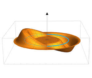
Figure 3. Example of a planar vortex ring  ${\mathcal {L}}_0$ (in cyan) subject to a localized twist phase prescribed by (2.5): $f(r)$ is given by (2.6), and $g(s)$ is given here by a periodic sinusoidal function along the nodal line ${\mathcal {L}}_0$. (a) Visualization of $\displaystyle \theta _{tw}$ (not to scale). (b) Visualization of the twist ribbon $R$ at points very close to the nodal line (not to scale); note that according to (2.6), the twist goes to zero when $r\ge \xi$.
4.1. Proof of writhe production by twist relaxation
The writhing number  $Wr$ of ${\mathcal {L}}$ is a global geometric property that measures the amount of coiling and distortion of ${\mathcal {L}}$ in space (Fuller Reference Fuller1971). A plane curve has zero writhe, but in general $Wr$ can take any real value. Writhe is measured by the solid angle spanned by the tangent indicatrix of ${\mathcal {L}}$ on the unit sphere, and it can be identified with the geometric phase acquired by the particles travelling along ${\mathcal {L}}$. Indeed, the geometric phase is the phase acquired by a system when its Hamiltonian depends on a parameter that varies in space or time. By identifying such a parameter with the unit tangent ${\boldsymbol {\hat T}}$ to ${\mathcal {L}}$, the evolution of ${\mathcal {L}}$ determines (by the tangent map) a closed curve on the Gauss sphere $S^2$. The geometric phase is thus measured by the solid angle swept out by the tangent indicatrix on $S^2$. This phase is gauge-invariant under $SO(3)$, i.e. under the choice of a fixed axis in $\mathbb {R}^3$.
An isolated defect such as a vortex ring has minimum configurational energy when both writhe  $Wr$ and total twist $Tw$ are identically zero. Since GPE defects are states of zero helicity (Salman Reference Salman2017; Kedia et al. Reference Kedia, Kleckner, Scheeler and Irvine2018), an isolated defect has self-linking number $Sl=Wr+Tw=0$, a condition that persists during the evolution (Sumners et al. Reference Sumners, Cruz-White and Ricca2021). This condition is evidently preserved also at minimum energy. For classical systems, such as elastic strings, twist relaxation under conservation of $Sl=0$ determines spontaneous production of writhe (see figure 4). Here, we demonstrate that the same relaxation process occurs for quantum defects. With reference to the two cases above, we prove the following result.
Theorem 4.1 Let  ${\mathcal {L}}$ denote a closed space curve that is a nodal line of a quantum defect in isolation; the defect is subject to a twist phase $\displaystyle \theta _{tw}$ localized in ${\mathcal {T}}({\mathcal {L}})$. Suppose that at $t=0$ we have $Tw\neq 0$, $Wr=0$ and $\nabla ^2\displaystyle \theta _{tw}>0$ in ${\mathcal {T}}({\mathcal {L}})$. Under conservation of zero helicity, we have
 \begin{align} Tw \to -Wr\ (\mathrm{mod}\; 2)\ \quad \textrm{as }t\uparrow\;\forall t>0 . \end{align}
Proof. According to (2.1), if  $\nabla ^2\displaystyle \theta _{tw}>0$, then the Hamiltonian is non-Hermitian and the system is linearly unstable. Thus in the case of localized twist phase, we have
 \begin{equation} Tw=\frac1{2{\rm \pi}}\oint_{{\mathcal{L}}}\displaystyle \boldsymbol{\nabla} \displaystyle \theta_{tw}\boldsymbol{\cdot}{\boldsymbol{\hat T}}\,\mathrm{d} s\neq0 , \end{equation}
and along  ${\mathcal {L}}$ we can take
 \begin{equation} \nabla^2\displaystyle \theta_{tw}\approx\frac{{\rm d}|\displaystyle \boldsymbol{\nabla} \displaystyle \theta_{tw}|}{{\rm d} s}=\frac{{\rm d}^2\displaystyle \theta_{tw}}{{\rm d} s^2}>0,\quad \forall\,t>0 \end{equation}
(in the healing region  $\mathrm {d}^2\displaystyle \theta _{tw}/\mathrm {d} r^2\approx 0$). We have two cases. (i) In one case $\displaystyle \theta _{tw}$ is discontinuous along ${\mathcal {L}}$: in this case the product $u_{tw}{\boldsymbol {\hat T}}$ must be multi-valued, because $\textrm {d}|\displaystyle \boldsymbol {\nabla } \displaystyle \theta _{tw}|/\textrm {d}s>0$ determines two different values of $|\displaystyle \boldsymbol {\nabla } \displaystyle \theta _{tw}|$ on a closed curve (say at the origin and after a full turn on ${\mathcal {L}}$). If ${\boldsymbol {\hat T}}$ remained constant with respect to a fixed direction ${\boldsymbol {\hat z}}$, then $E_{tw}\propto u_{tw}^2$ would be also multi-valued, evidently inadmissible from a physical viewpoint (the condensate cannot have two different energy values at a single point). Therefore ${\boldsymbol {\hat T}}$ must change direction. (ii) In the other case $\displaystyle \theta _{tw}$ is continuous along ${\mathcal {L}}$: in this case the instability relation (2.4) and the change of sign of $\nabla ^2\displaystyle \theta _{tw}$ along ${\mathcal {L}}$ imply the change in direction of ${\boldsymbol {\hat T}}$. Let us denote by ${\boldsymbol {\varOmega }}$ the spatial angular velocity of ${\boldsymbol {\hat T}}$ with respect to ${\boldsymbol {\hat z}}$. Interpreting the arc length variation of ${\boldsymbol {\hat T}}$ along ${\mathcal {L}}$ in terms of rigid body rotation of the Frenet triad, we have
 \begin{equation} {\boldsymbol{\hat T}}'= {\boldsymbol{\varOmega}}\times{\boldsymbol{\hat T}}, \quad \forall\,t>0, \end{equation}
where prime denotes arc length derivative. By taking the cross-product of (4.4) with  ${\boldsymbol {\hat T}}$, using a standard vector identity, and multiplying everything by ${\boldsymbol {\hat z}}$, we have
 \begin{equation} {\boldsymbol{\hat z}}\boldsymbol{\cdot}({\boldsymbol{\hat T}}\times{\boldsymbol{\hat T}}')= {\boldsymbol{\hat z}}\boldsymbol{\cdot}[{\boldsymbol{\varOmega}}-({\boldsymbol{\varOmega}}\boldsymbol{\cdot}{\boldsymbol{\hat T}}){\boldsymbol{\hat T}}]. \end{equation}
Let  ${\boldsymbol {\varOmega }}_\parallel$ and ${\boldsymbol {\varOmega }}_\perp$ denote the parallel and perpendicular contributions of ${\boldsymbol {\varOmega }}$ to ${\boldsymbol {\hat z}}$; from the right-hand side of (4.5), we have
 \begin{equation} {\boldsymbol{\hat z}}\boldsymbol{\cdot}({\boldsymbol{\hat T}}\times{\boldsymbol{\hat T}}')=\varOmega_\parallel{-}{\boldsymbol{\hat z}}\boldsymbol{\cdot}{\boldsymbol{\hat T}}({\boldsymbol{\varOmega}}_\perp\boldsymbol{\cdot}{\boldsymbol{\hat T}}) -\varOmega_\parallel({\boldsymbol{\hat z}}\boldsymbol{\cdot}{\boldsymbol{\hat T}})^2 , \end{equation}
or
 \begin{equation} \varOmega_\parallel{=}\frac{{\boldsymbol{\hat z}}\boldsymbol{\cdot}({\boldsymbol{\hat T}}\times{\boldsymbol{\hat T}}')}{1-({\boldsymbol{\hat z}}\boldsymbol{\cdot}{\boldsymbol{\hat T}})^2} + \frac{{\boldsymbol{\hat z}}\boldsymbol{\cdot}{\boldsymbol{\hat T}} ({\boldsymbol{\varOmega}}_\perp\boldsymbol{\cdot}{\boldsymbol{\hat T}})}{1-({\boldsymbol{\hat z}}\boldsymbol{\cdot}{\boldsymbol{\hat T}})^2} , \end{equation}
where  $\varOmega _\parallel =|{\boldsymbol {\varOmega }}_\parallel |$. Now we take advantage of the gauge invariance of (4.4) under ${\boldsymbol {\varOmega }}\to {\boldsymbol {\varOmega }}+({\boldsymbol {\varOmega }}\boldsymbol {\cdot }{\boldsymbol {\hat T}}){\boldsymbol {\hat T}}$. From that equation and the gauge freedom of ${\boldsymbol {\varOmega }}$, we have
 \begin{equation} {\boldsymbol{\hat T}}'= [{\boldsymbol{\varOmega}}+({\boldsymbol{\varOmega}}\boldsymbol{\cdot}{\boldsymbol{\hat T}}){\boldsymbol{\hat T}}]\times{\boldsymbol{\hat T}}, \end{equation}
and choose  ${\boldsymbol {\varOmega }}_\perp \boldsymbol {\cdot }{\boldsymbol {\hat T}}=({\boldsymbol {\hat z}}\times {\boldsymbol {\hat T}}')\boldsymbol {\cdot }{\boldsymbol {\hat T}}$; we can thus rewrite (4.7) as
 \begin{equation} \varOmega_\parallel=\frac{{\boldsymbol{\hat z}}\boldsymbol{\cdot}({\boldsymbol{\hat T}}\times{\boldsymbol{\hat T}}')}{1-({\boldsymbol{\hat z}}\boldsymbol{\cdot}{\boldsymbol{\hat T}})^2} - \frac{{\boldsymbol{\hat z}}\boldsymbol{\cdot}{\boldsymbol{\hat T}} ({\boldsymbol{\hat z}}\boldsymbol{\cdot}{\boldsymbol{\hat T}}\times{\boldsymbol{\hat T}}')}{1-({\boldsymbol{\hat z}}\boldsymbol{\cdot}{\boldsymbol{\hat T}})^2} . \end{equation}
By standard decomposition of total twist in geometric terms, we have  $Tw={\mathcal {T}}+{\mathcal {N}}$, where ${\mathcal {T}}$ is the normalized total torsion, and ${\mathcal {N}}$ the intrinsic twist given by the framing ${\boldsymbol {\hat U}}$ on ${\mathcal {L}}$ (Moffatt & Ricca Reference Moffatt and Ricca1992). By Lemma A.1 of Appendix A, we can write ${\mathcal {T}}$ in terms of ${\boldsymbol {\hat z}}$, and by Lemma A.2 we can see that the integral of (4.9) is the writhing number $\mathrm {mod}\;2$, i.e.
 \begin{equation} {-\frac1{2{\rm \pi}}}\oint_{{\mathcal{L}}}\varOmega_\parallel\,\mathrm{d} s={-}Wr\ (\mathrm{mod}\; 2). \end{equation}
Hence the rotation of  ${\boldsymbol {\hat T}}$ converts the initial localized phase twist to a geometric phase given by the production of writhe. Since (4.9) takes into account the sole rotation of ${\boldsymbol {\hat T}}$ in space without involving the ${\boldsymbol {\hat U}}$ framing on ${\mathcal {L}}$, by (4.2) we have
 \begin{equation} Tw \to -Wr\ (\mathrm{mod}\; 2)\ \quad \textrm{as }t\uparrow\;\forall t>0\ , \end{equation}
as stated.

Figure 4. Spontaneous production of writhe by twist energy relaxation: (a) elastic loop (adapted from Wadati & Tsuru Reference Wadati and Tsuru1986); (b) skyrmion soliton solution (adapted from Battye & Sutcliffe Reference Battye and Sutcliffe1998).
Remark 4.2 The gauge freedom is reflected in the free choice of  ${\boldsymbol {\hat z}}$ in space, hence fixing the gauge is equivalent to fixing ${\boldsymbol {\hat z}}$ in $\mathbb {R}^3$. It can be shown that the choice of taking ${\boldsymbol {\varOmega }}_\perp \boldsymbol {\cdot }{\boldsymbol {\hat T}}=({\boldsymbol {\hat z}}\times {\boldsymbol {\hat T}}')\boldsymbol {\cdot }{\boldsymbol {\hat T}}$ is equivalent to assuming ${\boldsymbol {\varOmega }}\boldsymbol {\cdot }{\boldsymbol {\hat T}}=-\varOmega _\parallel$.
Remark 4.3 The conversion of twist to writhe given by the rotation of  ${\boldsymbol {\hat T}}$ is due to the distortion of ${\mathcal {L}}$ in space and the defect energy redistribution, with production of writhing energy density $-\mathrm {i}\,\nabla ^2{\displaystyle \theta _{tw}}|\displaystyle \psi _{{1}}|^2$ to cancel out the imaginary term in (2.1).
5. Two examples of defect ring subject to localized twist
Two examples of the effect of the localized twist that provide interesting test cases for laboratory experiments are presented for illustration.
Increasing twist. Consider a vortex ring  ${\mathcal {L}}_0$ subject to localized twist with $\textrm {d}|\boldsymbol {\nabla }\theta _{tw}|/\textrm {d}s>0$ along ${\mathcal {L}}_0$. Since $\nabla ^2\displaystyle \theta _{tw} > 0$, the vortex becomes unstable. At the point of twist injection, where the ribbon closes on itself, twist flux is maximum. Relaxation of twist determines defect distortion, with consequential production of writhe. Stability is restored eventually when the imaginary part of the energy functional (2.1) is absorbed by the defect deformation. Below the critical twist threshold imposed by the speed of sound (cf. (2.7)), the defect may coil up and fold over, with possible phase fragmentation and defect reconnection to produce small-scale vortex rings.
Oppositely signed twist. A limit case is represented by a vortex ring subject to localized, constant twist propagating with opposite sign in opposite directions from the point of injection. The Laplacian along the defect is different from zero, but the total flux is zero with source ( $\nabla ^2\displaystyle \theta _{tw} > 0$) and sink ( $\nabla ^2\displaystyle \theta _{tw} < 0$) contributions radiating away from the point of injection. These contributions may produce a distortion of the defect in space with simultaneous creation of positive and negative coiled regions while keeping total writhe equal to zero.
6. Conclusions
In this paper we have considered the physical effects of the superposition of an external twist phase on an isolated quantum vortex defect governed by the Gross–Pitaevskii equation. By relying on stability results obtained previously by the present authors (FR20), we have analysed the effects of global and local phase twist (§ 2) to demonstrate two results. (i) When the superposed phase is uniformly twisted everywhere in the condensate, a secondary defect is produced as a result of an Aharonov–Bohm type effect (§ 3). (ii) When the superposed phase twist is localized, i.e. it is confined in the tubular healing region of the nodal line, the defect undergoes a distortion due to the production of writhe by twist relaxation (§ 4). This mechanism, proved here for quantum systems, is analogous to the relaxation of supercoiled elastic strings in classical mechanics (Wadati & Tsuru Reference Wadati and Tsuru1986). Two simple examples are presented in § 5 to illustrate the physical effects of twist localization. These results rely on application of Kleinert's (Reference Kleinert2008) defect gauge theory for multi-valued potentials, and use of simple geometric results derived in Appendix A.
There are physical effects that may limit the amount of twist flux injected. On one hand, since  $\displaystyle \boldsymbol {\nabla } \displaystyle \theta _{tw}$ induces an axial velocity $u_a$ and this is limited by the speed of sound $c_s$ ( $u_a< c_s$), there must be an upper limit on the injected twist. Moreover, since a localized twist is confined to the tubular healing region, there must be also a natural limit given by the amount of particles that can be transported along the nodal line. Both these effects must play a part in the values of $\displaystyle \theta _{tw}$ that are physically realizable.
Our results shed new light on the physical effects of twist on defect dynamics. According to whether twist prescription is global or local, we may have production of new defects or twist relaxation with consequential geometric distortion of the original defect and creation of writhe. Indeed, writhe production corresponds to the generation of a geometric Berry phase (Hannay Reference Hannay1998; Chruscinski & Jamiolkowski Reference Chruscinski and Jamiolkowski2004). The examples presented in § 5 show that even under twist localization we can have quite different scenarios: either a change of shape through distortion of the defect in space, or, if twist exceeds a critical threshold, possible phase fragmentation and reconnection of the original defect with production of small-scale vortex rings. These conclusions, based on purely theoretical arguments, show the subtle role that topology and twist localization (or the lack of it) may play in the physics of condensates. In light of the most recent developments in condensed matter physics (Klawunn & Santos Reference Klawunn and Santos2009; Caputo et al. Reference Caputo, Bobrovska, Ballarini, Matuszewski, De Giorgi, Dominici, West, Pfeiffer, Gigli and Sanvitto2019; Saxena et al. Reference Saxena, Kevrekidis and Cuevas-Maraver2020; Bergholtz, Budich & Kunst Reference Bergholtz, Budich and Kunst2021), these results suggest new ways to produce secondary defects, or trigger configurational changes of existing defects, that may help to enhance physical properties for scientific purposes and technological applications.
Funding
R.L.R. wishes to acknowledge financial support from the National Natural Science Foundation of China (grant no. 11572005).
Declaration of interests
The authors declare no competing financial and non-financial interests in the preparation of this work.
Author contributions
The authors contributed equally to design the project, discuss the results and revise the manuscript.
Appendix A. Total torsion and writhing number in terms of ${\boldsymbol {\hat z}}$

Let  ${\mathcal {L}}$ be a smooth, closed space curve of unit tangent, normal and binormal given by the Frenet triad $\{{\boldsymbol {\hat T}},{\boldsymbol {\hat N}},{\boldsymbol {\hat B}}\}$, curvature $c=c(s)$ and torsion $\tau =\tau (s)$, all smooth functions of arc length $s$ of ${\mathcal {L}}$. We have the following.
Lemma A.1 Given a smooth, closed, space curve  ${\mathcal {L}}$ and a fixed axis ${\boldsymbol {\hat z}}$ in $\mathbb {R}^3$, we have
 \begin{equation}
{\mathcal{T}}=\frac1{2{\rm \pi}}\oint_{{\mathcal{L}}}\tau\,
\mathrm{d} s =\frac1{2{\rm \pi}}
\oint_{{\mathcal{L}}}\frac{({\boldsymbol{\hat
z}}\boldsymbol{\cdot}{\boldsymbol{\hat
T}})({\boldsymbol{\hat
z}}\boldsymbol{\cdot}{\boldsymbol{\hat
T}}\times{\boldsymbol{\hat T}}')} {1 -
({\boldsymbol{\hat z}}\boldsymbol{\cdot}{\boldsymbol{\hat
T}})^2}\,\mathrm{d} s .
\end{equation}
\begin{equation}
{\mathcal{T}}=\frac1{2{\rm \pi}}\oint_{{\mathcal{L}}}\tau\,
\mathrm{d} s =\frac1{2{\rm \pi}}
\oint_{{\mathcal{L}}}\frac{({\boldsymbol{\hat
z}}\boldsymbol{\cdot}{\boldsymbol{\hat
T}})({\boldsymbol{\hat
z}}\boldsymbol{\cdot}{\boldsymbol{\hat
T}}\times{\boldsymbol{\hat T}}')} {1 -
({\boldsymbol{\hat z}}\boldsymbol{\cdot}{\boldsymbol{\hat
T}})^2}\,\mathrm{d} s .
\end{equation}
Proof. Consider the unit vector decomposition  ${\boldsymbol {\hat z}}=({\boldsymbol {\hat z}}\boldsymbol {\cdot }{\boldsymbol {\hat T}}){\boldsymbol {\hat T}}+({\boldsymbol {\hat z}}\boldsymbol {\cdot }{\boldsymbol {\hat z}}_\perp ){\boldsymbol {\hat z}}_\perp$, where ${\boldsymbol {\hat z}}_\perp$ is a unit vector orthogonal to ${\boldsymbol {\hat T}}$ on ${\mathcal {L}}$. By using $({\boldsymbol {\hat z}}\boldsymbol {\cdot }{\boldsymbol {\hat z}}_\perp )^2=1-({\boldsymbol {\hat z}}\boldsymbol {\cdot }{\boldsymbol {\hat T}})^2$, we have
 \begin{equation} {\boldsymbol{\hat z}}_\perp{=}\frac{{\boldsymbol{\hat z}}-({\boldsymbol{\hat z}}\boldsymbol{\cdot}{\boldsymbol{\hat T}}){\boldsymbol{\hat T}}}{\sqrt{1-({\boldsymbol{\hat z}}\boldsymbol{\cdot}{\boldsymbol{\hat T}})^2}} . \end{equation}
After some straightforward algebra, we have
 \begin{equation} ({\boldsymbol{\hat z}}_\perp{\times}{\boldsymbol{\hat z}}_\perp^\prime)\boldsymbol{\cdot}{\boldsymbol{\hat T}} =\frac{({\boldsymbol{\hat z}}\boldsymbol{\cdot}{\boldsymbol{\hat T}})({\boldsymbol{\hat z}}\boldsymbol{\cdot}{\boldsymbol{\hat T}}\times {\boldsymbol{\hat T}}')}{1 - ({\boldsymbol{\hat z}}\boldsymbol{\cdot}{\boldsymbol{\hat T}})^2}. \end{equation}
By recalling the definition of total twist (Moffatt & Ricca Reference Moffatt and Ricca1992), we have
 \begin{equation} Tw=\frac1{2{\rm \pi}}\oint_{{\mathcal{L}}}({\boldsymbol{\hat z}}_\perp{\times}{\boldsymbol{\hat z}}_\perp^\prime)\boldsymbol{\cdot}{\boldsymbol{\hat T}}\, \mathrm{d} s =\frac1{2{\rm \pi}}\oint_{{\mathcal{L}}}(\tau+\alpha')\, \mathrm{d} s, \end{equation}
where  $\alpha =\alpha (s)$ is the rotation angle of the intrinsic twist $\mathcal {N}$; from (A4) we have
 \begin{equation} \varkappa=\frac{({\boldsymbol{\hat z}}\boldsymbol{\cdot}{\boldsymbol{\hat T}})({\boldsymbol{\hat z}}\boldsymbol{\cdot}{\boldsymbol{\hat T}}\times{\boldsymbol{\hat T}}')}{1 - ({\boldsymbol{\hat z}}\boldsymbol{\cdot}{\boldsymbol{\hat T}})^2}=\tau+\alpha' . \end{equation}
We want to prove that  $\varkappa =k\tau$, with $k=1$. First we prove that $\varkappa =0\Leftrightarrow \tau =0$. (i) If $\varkappa =0$, then ${\boldsymbol {\hat z}}\boldsymbol {\cdot }{\boldsymbol {\hat T}}=0$ or ${\boldsymbol {\hat z}}\boldsymbol {\cdot }{\boldsymbol {\hat T}}\times {\boldsymbol {\hat T}}'=0$. In the first case, since ${\boldsymbol {\hat z}}$ is fixed in space, ${\boldsymbol {\hat z}}\boldsymbol {\cdot }{\boldsymbol {\hat T}}=0$ iff ${\boldsymbol {\hat z}}\perp {\boldsymbol {\hat T}}$, which means that ${\mathcal {L}}$ must be planar with $\tau =0$. In the second case, ${\boldsymbol {\hat z}}\boldsymbol {\cdot }{\boldsymbol {\hat T}}\times {\boldsymbol {\hat T}}'=0$ iff (by Frenet–Serret equations) $c\,{\boldsymbol {\hat z}}\boldsymbol {\cdot }{\boldsymbol {\hat B}}=0$. Since ${\mathcal {L}}$ is closed, $c\neq 0$ (almost everywhere) and so ${\boldsymbol {\hat z}}\boldsymbol {\cdot }{\boldsymbol {\hat B}}=0$; this means that $({\boldsymbol {\hat z}}\boldsymbol {\cdot }{\boldsymbol {\hat B}})'=0$ iff $-\tau \,{\boldsymbol {\hat z}}\boldsymbol {\cdot }{\boldsymbol {\hat N}}=0$. If $\tau \neq 0$, then ${\boldsymbol {\hat z}}\boldsymbol {\cdot }{\boldsymbol {\hat N}}=0$, that is ${\boldsymbol {\hat z}}\perp {\boldsymbol {\hat B}}$ and ${\boldsymbol {\hat z}}\perp {\boldsymbol {\hat N}}$, so that ${\boldsymbol {\hat z}}\parallel {\boldsymbol {\hat T}}$. However, since ${\boldsymbol {\hat z}}'=0$, we must have $({\boldsymbol {\hat z}}\boldsymbol {\cdot }{\boldsymbol {\hat N}})'={\boldsymbol {\hat z}}\boldsymbol {\cdot }{\boldsymbol {\hat N}}'=-c\,{\boldsymbol {\hat z}}\boldsymbol {\cdot }{\boldsymbol {\hat T}}+\tau \,{\boldsymbol {\hat z}}\boldsymbol {\cdot }{\boldsymbol {\hat B}}=0$, i.e. ${\boldsymbol {\hat z}}\boldsymbol {\cdot }{\boldsymbol {\hat T}}=0$, which contradicts the assumption; hence $\tau =0$. (ii) If $\tau =0$, then ${\mathcal {L}}$ is planar. We can always choose ${\boldsymbol {\hat z}}$ such that ${\boldsymbol {\hat z}}\boldsymbol {\cdot }{\boldsymbol {\hat T}}=0$. Hence $\varkappa =0$.
From (i) and (ii) above, and (A5), we thus have  $\varkappa =k\tau =\tau +\alpha '$, that is $\alpha '=(k-1)\tau$; however, this cannot be true because $\alpha '$ is independent of torsion. Hence $\alpha '=0$ and $k=1$, that is $\varkappa =\tau$; hence, using (A5) we have the statement (A1).
The writhing number  $Wr$ is measured by the solid angle spanned by the tangent indicatrix ${\mathcal {L}}^*$ of ${\mathcal {L}}$ on the unit sphere $S^2$ (Fuller Reference Fuller1971), and can thus be interpreted as the flux of ${\boldsymbol {\hat T}}$ through the surface spanned by ${\mathcal {L}}^*$ on $S^2$. We have the following result.
Lemma A.2 Given a smooth closed space curve  ${\mathcal {L}}$ and a fixed axis ${\boldsymbol {\hat z}}$ in $\mathbb {R}^3$, we have
 \begin{equation}
Wr=\frac1{2{\rm \pi}}\oint_{{\mathcal{L}}}\left[
\frac{{\boldsymbol{\hat
z}}\boldsymbol{\cdot}{\boldsymbol{\hat
T}}\times{\boldsymbol{\hat T}}'}{1 - ({\boldsymbol{\hat
z}}\boldsymbol{\cdot}{\boldsymbol{\hat T}})^2}
-\frac{({\boldsymbol{\hat
z}}\boldsymbol{\cdot}{\boldsymbol{\hat
T}})({\boldsymbol{\hat
z}}\boldsymbol{\cdot}{\boldsymbol{\hat
T}}\times{\boldsymbol{\hat T}}')}{1 -
({\boldsymbol{\hat z}}\boldsymbol{\cdot}{\boldsymbol{\hat
T}})^2}\right]\,\mathrm{d} s \quad (\mathrm{mod}\; 2)
. \end{equation}
\begin{equation}
Wr=\frac1{2{\rm \pi}}\oint_{{\mathcal{L}}}\left[
\frac{{\boldsymbol{\hat
z}}\boldsymbol{\cdot}{\boldsymbol{\hat
T}}\times{\boldsymbol{\hat T}}'}{1 - ({\boldsymbol{\hat
z}}\boldsymbol{\cdot}{\boldsymbol{\hat T}})^2}
-\frac{({\boldsymbol{\hat
z}}\boldsymbol{\cdot}{\boldsymbol{\hat
T}})({\boldsymbol{\hat
z}}\boldsymbol{\cdot}{\boldsymbol{\hat
T}}\times{\boldsymbol{\hat T}}')}{1 -
({\boldsymbol{\hat z}}\boldsymbol{\cdot}{\boldsymbol{\hat
T}})^2}\right]\,\mathrm{d} s \quad (\mathrm{mod}\; 2)
. \end{equation}
Proof. Let us identify the polar axis on  $S^2$ with the ${\boldsymbol {\hat z}}$-axis, fixed in $\mathbb {R}^3$. From Binysh & Alexander (Reference Binysh and Alexander2018, equation (14)), without loss of generality we take ${\boldsymbol {\hat n}}_\infty \equiv {\boldsymbol {\hat z}}$; we have
 \begin{equation} Wr=\frac1{2{\rm \pi}}\oint_{{\mathcal{L}}}\frac{{\boldsymbol{\hat z}}\boldsymbol{\cdot}{\boldsymbol{\hat T}}\times{\boldsymbol{\hat T}}'}{1 + {\boldsymbol{\hat z}}\boldsymbol{\cdot}{\boldsymbol{\hat T}}}\,\mathrm{d} s \quad (\mathrm{mod}\; 2). \end{equation}
By multiplying and dividing the integrand above by  $(1-{\boldsymbol {\hat z}}\boldsymbol {\cdot }{\boldsymbol {\hat T}})$, we have
 \begin{equation} \frac{{\boldsymbol{\hat z}}\boldsymbol{\cdot}{\boldsymbol{\hat T}}\times{\boldsymbol{\hat T}}'}{1 + {\boldsymbol{\hat z}}\boldsymbol{\cdot}{\boldsymbol{\hat T}}} =\frac{(1-{\boldsymbol{\hat z}}\boldsymbol{\cdot}{\boldsymbol{\hat T}})({\boldsymbol{\hat z}}\boldsymbol{\cdot}{\boldsymbol{\hat T}}\times{\boldsymbol{\hat T}}')}{1 - ({\boldsymbol{\hat z}}\boldsymbol{\cdot}{\boldsymbol{\hat T}})^2} =\frac{{\boldsymbol{\hat z}}\boldsymbol{\cdot}{\boldsymbol{\hat T}}\times{\boldsymbol{\hat T}}'}{1 - ({\boldsymbol{\hat z}}\boldsymbol{\cdot}{\boldsymbol{\hat T}})^2} -\frac{({\boldsymbol{\hat z}}\boldsymbol{\cdot}{\boldsymbol{\hat T}})\left({\boldsymbol{\hat z}}\boldsymbol{\cdot}{\boldsymbol{\hat T}}\times{\boldsymbol{\hat T}}'\right)}{1 - ({\boldsymbol{\hat z}}\boldsymbol{\cdot}{\boldsymbol{\hat T}})^2} . \end{equation}
Substituting the right-hand side above into (A7), we have the statement.


 Open access