


1. Introduction
Aircraft engine manufacturers are striving to make aeroengines both cleaner and quieter to meet the stringent targets set by aviation advisory councils. On the one hand, to make gas-turbine combustors cleaner, flames typically operate in a lean regime. On the other hand, lean flames are sensitive to the turbulent environment of the combustor, which can result in significantly unsteady chemical and fluid dynamics, which, in turn, can add to sound generation via direct and indirect mechanisms. In the combustor, two categories of noise can be identified. Direct noise is caused by the unsteady flickering of the flame, which leads to a volumetric expansion and contraction of the flow which, in turn, generates acoustic waves. If these acoustic waves propagate downstream of the combustor, these waves are perceived as noise (e.g. Strahle Reference Strahle1976). Direct noise is a well-studied phenomenon both experimentally and numerically, as reviewed by Ihme (Reference Ihme2017). Indirect noise is caused by a different mechanism, that is, the acceleration of flow inhomogeneities through the nozzle downstream of the combustor (e.g. Williams & Howe Reference Williams and Howe1975; Strahle Reference Strahle1976; Marble & Candel Reference Marble and Candel1977; Cumpsty Reference Cumpsty1979; Polifke, Paschereit & Döbbeling Reference Polifke, Paschereit and Döbbeling2001; Morgans & Duran Reference Morgans and Duran2016; Magri, O'Brien & Ihme Reference Magri, O'Brien and Ihme2016). Indirect noise generated by inhomogeneities in temperature is typically referred to as entropy noise (Cuadra Reference Cuadra1967; Marble & Candel Reference Marble and Candel1977; Bake et al. Reference Bake, Richter, Mühlbauer, Kings, Röhle, Thiele and Noll2009; Duran & Moreau Reference Duran and Moreau2013), whereas indirect noise generated by inhomogeneities in the composition is referred to as compositional noise (Magri et al. Reference Magri, O'Brien and Ihme2016; Magri Reference Magri2017). Indirect noise can also affect the combustor's stability. If the acoustic waves generated from inhomogeneities reflect off the components downstream of the combustor, they can synchronize constructively with the heat released by the flames, which can lead to thermoacoustic instabilities (Polifke et al. Reference Polifke, Paschereit and Döbbeling2001; Goh & Morgans Reference Goh and Morgans2013; Motheau, Nicoud & Poinsot Reference Motheau, Nicoud and Poinsot2014; Morgans & Duran Reference Morgans and Duran2016). These instabilities can cause a reduction in the engine lifetime and may also lead to structural failures (Dowling & Mahmoudi Reference Dowling and Mahmoudi2015). To understand and capture the key physical mechanisms of indirect noise in low-order models for the preliminary design of aircraft engines, substantial research has been carried out. Marble & Candel (Reference Marble and Candel1977) introduced a model to predict entropy noise for a compact nozzle flow, which was extended to non-compact nozzle flows by Leyko, Nicoud & Poinsot (Reference Leyko, Nicoud and Poinsot2009) and Duran & Moreau (Reference Duran and Moreau2013), among others. These models assumed the flow to have a homogeneous composition, which can be approximated as a single component flow. However, factors such as air cooling and improper mixing can generate inhomogeneities in the flow composition. The models of homogeneous flows were generalized to multicomponent flows to calculate the indirect noise caused by compositional inhomogeneities in both compact and non-compact nozzle flows by Magri et al. (Reference Magri, O'Brien and Ihme2016) and Magri (Reference Magri2017), and were reviewed in Magri, Schmid & Moeck (Reference Magri, Schmid and Moeck2023). These studies were further generalized to flows with entropy generation due to flow dissipation (e.g. De Domenico, Rolland & Hochgreb Reference De Domenico, Rolland and Hochgreb2019; Jain & Magri Reference Jain and Magri2022a,Reference Jain and Magrib, Reference Jain and Magri2023; Guzmán-Iñigo et al. Reference Guzmán-Iñigo, Yang, Gaudron and Morgans2022).
In the aforementioned studies the flow is assumed to be chemically frozen. Giusti, Magri & Zedda (Reference Giusti, Magri and Zedda2019) performed a large-eddy simulation study on a realistic aero-engine combustor. They showed that some flow inhomogeneities are chemically reacting when they leave the combustor and enter the nozzle guide vane. The chemical reaction produces both changes in composition and entropy fluctuations. Patki, Acharya & Lieuwen (Reference Patki, Acharya and Lieuwen2022) modelled the entropy generation mechanisms from exothermic chemical reactions in laminar premixed flames, but physical mechanisms for sound generation were not investigated.
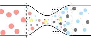
The overarching objective of this work is to derive from first principles the governing equations to model sound generation (indirect noise) in nozzles generated by reacting flow inhomogeneities. We will focus on weakly reacting flows, in which the volume of the reacting pocket of flow is small with respect to the volume of the mean flow (figure 1). We compute the effect of reacting inhomogeneities with hydrogen and methane fuels. Hydrogen is the potential future of energy and aviation because of its carbon-free reaction (Sürer & Arat Reference Sürer and Arat2018; Yusaf et al. Reference Yusaf, Fernandes, Abu Talib, Altarazi, Alrefae, Kadirgama, Ramasamy, Jayasuriya, Brown and Mamat2022). Because the combustion of hydrogen-based fuel blends is achieved in a lean regime, they are susceptible to incomplete combustion as compared with hydrocarbon fuels (Hosseini & Butler Reference Hosseini and Butler2020). Methane is the main component of natural gases, which have been widely used in stationary gas turbines for power generation (Lefebvre & Ballal Reference Lefebvre and Ballal2010). Specifically, the goals of this work are to: (i) propose a physics-based model to predict acoustics generated by the acceleration of chemically reacting inhomogeneities; (ii) analyse the source of sound that generate indirect noise; (iii) compute and analyse the transfer functions in subsonic flows; and (iv) generalize the model to supersonic nozzle flows. To achieve these goals, two convergent–divergent nozzles are numerically investigated. The paper is structured as follows. Section 2 introduces the physical model and identifies the sources of sound. Section 3 describes the chemistry model and the sources of sound. Sections 4 and 5 show the acoustic transfer functions in a subsonic and supersonic flow regime, respectively. Conclusions end the paper.

Figure 1. Reacting flow schematic with an example of combustion of fuel with products  $P_1$ and $P_2$.
2. Mathematical model
In this section, we model a multi-component chemically reacting flow through a nozzle. We assume a multi-component flow that is dominated by a quasi-one-dimensional dynamics and has no viscous dissipation. The flow is adiabatic with negligible diffusion effects. We assume the chemical reactions to be nearly completed at the exit of the combustor with pockets of unburnt fuel-lean mixture. The reacting pockets occupy a small volume as compared with the mean flow. With these assumptions, the conservation equations of mass, momentum, energy and species are (Chiu & Summerfield Reference Chiu and Summerfield1974)
 \begin{gather} \frac{{\rm D}\rho}{{\rm D}t} + \rho\frac{\partial u}{\partial x} + \frac{\rho u}{A}\frac{{\rm d}A}{{\rm d}\kern0.7pt x} = {\dot{S}_m}, \end{gather}
 \begin{gather}\frac{{\rm D}u}{{\rm D}t} + \frac{1}{\rho}\frac{\partial p}{\partial x} = {\dot{S}_M}, \end{gather}
 \begin{gather}T\frac{{\rm D}s}{{\rm D}t} = {\dot{S}_s}, \end{gather}
 \begin{gather}\frac{{\rm D}Y_i}{{\rm D}t} = \dot{S_Y}, \end{gather}
where  $\rho$ is the density, $x$ is the axial distance, $t$ is the time, $u$ is the flow velocity, $A$ is the area of the nozzle cross-section, $p$ is the pressure, $T$ is the temperature and $s$ is the entropy ( $s = \sum _{i=1}^N s_{i} Y_i$). The flow is assumed to consist of $N$ species with mass fractions $Y_i$. The right-hand side terms of (2.1)–(2.4) are the source terms. We assume no mass generation, i.e. $\dot {S}_m = 0$. The effects of body forces and friction are neglected, i.e. $\dot {S}_M = 0$. The chemical reaction in the flow adds to the energy generation through the entropy source term
 \begin{equation} \dot{S}_s ={-} \sum_{i=1}^N \left(\frac{\mu_i}{W_i}\right) \frac{{\rm D}Y_i}{{\rm D}t},\end{equation}
where  $\mu _i = W_i({\partial h}/{\partial Y_i}) = W_i({\partial g}/{\partial Y_i})$ is the chemical potential, $W_i$ is the molar mass, $h = \sum _{i=1}^N h_{i} Y_i$ is the specific enthalpy and $g = h - T s$ is the specific Gibbs energy. The species source term is
 \begin{equation} \dot{S_Y} = \frac{1}{\rho}\dot\omega_i, \end{equation}
where  $\dot \omega _i$ is the rate of production (or consumption) of species $i$ by chemical reaction. These equations are closed by the Gibbs equation
 \begin{equation} T\,{{\rm d}s} = {\rm d}h - \frac{{\rm d}p}{\rho} - \sum_{i=1}^N \left(\frac{\mu_i}{W_i}\right) {\rm d}Y_i . \end{equation}
The gases are assumed to be ideal and calorically perfect, therefore
 \begin{equation} h = c_p(T - T^o), \quad c_p=\frac{\gamma}{\gamma - 1}R, \end{equation}
where  $R = \mathcal {R}\sum _{i=1}^N Y_i/W_i$ is the specific gas constant of the mixture, $\mathcal {R}$ is the universal gas constant, $T^o$ is the temperature of the reference state, $\gamma = c_p/c_v$ is the heat-capacity ratio and $c_p$ and $c_v$ are the specific heat capacities at constant pressure and constant volume, respectively, given by
 \begin{equation} c_p = \sum_{i=1}^N c_{p,i} Y_i, \quad c_v = \sum_{i=1}^N c_{v,i} Y_i. \end{equation}
Using (2.7), (2.8a,b),  $\mu _i/W_i = g_i = h_i - T s_i$ and the equation of state, $p=\rho R T$, the Gibbs equation becomes
 \begin{equation} \frac{{\rm d}s}{c_p} = \frac{{\rm d}p}{\gamma p} - \sum_{i=1}^N\left(\aleph_{1,i} + \psi_{1,i}\right){\rm d}Y_i, \end{equation}
where
 \begin{gather} \aleph_{1,i} = \frac{1}{\gamma - 1}\frac{{\rm d}\log\gamma}{{\rm d}Y_i} + \frac{T^o}{T} \frac{{\rm d}\log c_p}{{\rm d}Y_i}, \end{gather}
 \begin{gather}\psi_{1,i} = \frac{1}{c_p T} \left(\frac{\mu_i}{W_i} - \Delta h^o_{f,i}\right), \end{gather}
where  $\Delta h^o_{f,i}$ is the enthalpy of formation of the $i$th species, $\aleph _{1,i}$ and $\psi _{1,i}$ are the heat-capacity factor and chemical-potential functions, respectively. Replacing (2.9a,b) into (2.11)–(2.12) yields
 \begin{equation} \frac{{\rm d}\log\gamma}{{\rm d}Y_{i}} = \frac{1}{c_p}\sum_{j=1}^N c_{p_j}\frac{{\rm d}Y_j}{{\rm d}Y_i} - \frac{1}{c_v}\sum_{j=1}^N c_{v_j}\frac{{\rm d}Y_j}{{\rm d}Y_i}. \end{equation}
For  $i\neq j$, in a chemically reacting flow, ${\rm d}Y_i/{\rm d}Y_j$ depends on the stoichiometric coefficients; however, in a chemically frozen flow, ${\rm d}Y_i/{\rm d}Y_j = 0$. We exploit (2.13) to physically interpret the results for a binary mixture in § 3. With chemical reactions, it is simpler to work in the mass fraction domain, as opposed to the mixture fraction domain (e.g. Magri Reference Magri2017; Jain & Magri Reference Jain and Magri2023), which is the approach we take here. For completeness, the heat-capacity factor and chemical-potential functions defined in Magri (Reference Magri2017) are related to the factor $\aleph _{1,i}$ and $\psi _{1,i}$ of this work by
 \begin{equation} \aleph = \sum_{i=1}^N\aleph_{1,i} \frac{{\rm d}Y_i}{{\rm d}Z},\quad \psi = \sum_{i=1}^N \psi_{1,i}\frac{{\rm d}Y_i}{{\rm d}Z}. \end{equation}
2.1. Linearization
We model the acoustics as linear perturbations to a mean flow. We assume the nozzle cut-on frequency to be sufficiently large for the acoustics to be quasi-one-dimensional (e.g. Marble & Candel Reference Marble and Candel1977; Duran & Moreau Reference Duran and Moreau2013; Magri Reference Magri2017). For this, we decompose a generic flow variable as  $(.)\rightarrow {\overline {(.)}}(x) + \epsilon (.)^{\prime }(x,t)$, where ${\overline {(.)}}(x)$ is the steady mean-flow component, and $\epsilon (.)^{\prime }(x,t)$ is the first-order perturbation with $\epsilon \to 0$. On grouping the steady mean-flow terms, the mean-flow equations are
 \begin{equation} d(\bar{\rho}\bar{u} A) = 0,\quad d(\bar{p} + \bar{\rho}\bar{u}^2) = 0. \end{equation}
We assume that the mean flow has no dissipation, and consists of non-reacting constituents. The reaction rates of the mean-flow quantities are zero,  $\overline {\dot {\omega _i}} = 0$. Therefore
 \begin{equation} {\rm d}\bar{s} = 0,\quad {\rm d}\bar{Y}_i = 0. \end{equation}
By grouping the first-order terms, we obtain the equations that govern the acoustics and flow inhomogeneities
 \begin{gather} \frac{\bar{{\rm D}}}{{\rm D}t}\frac{\rho^{\prime}}{\bar{\rho}} + \bar{u} \frac{\partial}{\partial x}\left(\frac{u^{\prime}}{\bar{u}}\right) = 0, \end{gather}
 \begin{gather}\frac{\bar{{\rm D}}}{{\rm D}t}\left(\frac{u^{\prime}}{\bar{u}}\right) + \left(2\frac{u^{\prime}}{\bar{u}} + \frac{\rho^{\prime}}{\bar{\rho}}- \frac{p^{\prime}}{\bar p}\right) \left(\frac{\partial\bar{u}}{\partial x} \right) + \frac{1}{\bar{\gamma}}\left(\frac{\bar{u}}{\bar{M}^2}\right) \frac{\partial}{\partial x}\frac{p^{\prime}}{\bar{p}} = 0, \end{gather}
 \begin{gather}\bar{\rho}\frac{\bar{{\rm D}}}{{\rm D}t}\left(\frac{s^\prime}{\bar{c}_p}\right) ={-} \frac{1}{\bar{T}\bar{c}_p}\sum_{i=1}^N \left(\frac{\bar{\mu}_i}{\bar{W}_i}\right) \dot{\omega}_i^\prime, \end{gather}
 \begin{gather}\bar{\rho}\frac{\bar{{\rm D}}Y_i^\prime}{{\rm D}t} = {\dot{\omega}_i^\prime}, \end{gather}
where,  $\bar {{\rm D}}/{\rm D}t = \partial /\partial t + \bar {u}\partial /\partial x$. The heat released from the chemical reactions generates entropy fluctuations, $s^\prime /c_p$ (§ 2.1.1). Because the flow is assumed to be weakly reacting, non-conductive and adiabatic, we neglect the mean-flow heat transfer. For modelling the effect of heat transfer, the reader is referred to Yeddula, Gaudron & Morgans (Reference Yeddula, Gaudron and Morgans2021) and Yeddula, Guzmán-Iñigo & Morgans (Reference Yeddula, Guzmán-Iñigo and Morgans2022). To close the linear equations, we linearize the Gibbs equation (2.10) and take the material derivative and combine the first-order terms to yield
 \begin{equation} \frac{\bar{{\rm D}}}{{\rm D}t} \left(\frac{\rho^\prime}{\bar{\rho}}\right) = \frac{\bar{{\rm D}}}{{\rm D}t} \left(\frac{p^\prime}{\bar{\gamma}\bar{p}}\right) - \frac{\bar{{\rm D}}}{{\rm D}t}\left(\frac{s^\prime}{\bar{c}_p} \right) - \sum_{i=1}^N\left(\bar{\aleph}_{1,i} + \bar{\psi}_{1,i}\right)\frac{\bar{{\rm D}}Y_i^\prime}{{\rm D}t} - \frac{\gamma^\prime}{\bar{\gamma}}\frac{\bar{{\rm D}}}{{\rm D}t}{\log\bar{p}^{1/\bar{\gamma}}}, \end{equation}
where  $\gamma ^\prime = \sum _{i=1}^N({\rm d}\gamma /{\rm d}Y_i) Y_i^\prime$ is the perturbation to the heat-capacity ratio, which is a function of the species mass fractions, $Y_i$, only. The equation is integrated from an unperturbed state at $t \to -\infty$ to yield the density fluctuation as
 \begin{equation} \frac{\rho^\prime}{\bar{\rho}}= \frac{p^\prime}{\bar{\gamma}\bar{p}} - \frac{s^\prime}{\bar{c}_p} - \sum_{i=1}^N\left(\bar{\aleph}_{1,i} + \bar{\psi}_{1,i} + \bar{\phi}_{1,i}\right) Y_i^\prime - \bar{\varTheta}, \end{equation}
where
 \begin{equation} \bar{\phi}_{1,i} = \frac{{\rm d} \log\gamma}{{\rm d}Y_i}\log\tilde{p}^{{1/\bar{\gamma}}},\end{equation}
is the gamma-prime source of noise (Strahle Reference Strahle1976; Magri Reference Magri2017), and  $\tilde {p}$ is the normalized pressure, $\tilde {p} = p/p_{ref}$. We identify the chemical-reaction noise factor
 \begin{equation} \bar{\varTheta} = {\int_{-\infty}^{\tau}}\sum_{i=1}^N \phi_{1,i}\frac{{\rm D}Y_i^\prime}{{\rm D}t}\,{\rm d}t,\end{equation}
which physically depends on the variation of the heat-capacity ratio and the reaction rate,  $\dot {\omega }^\prime$, through (2.20). If the flow is chemically frozen ( ${\rm D}Y_i^\prime /{\rm D}t = 0$, thus, $\bar {\varTheta } = 0$), the density fluctuation (2.22) tends to that of the non-reacting compositional noise model of Magri (Reference Magri2017). On the one hand, if the flow is homogeneous, the density fluctuations depend only on pressure fluctuations. On the other hand, if the flow is inhomogeneous, the temperature and composition fluctuations also affect the density fluctuations. When these inhomogeneities accelerate through the nozzle, they contract and expand at a different rate than the mean flow, which generates momentum imbalance, and hence acoustic waves. The factors that are responsible for the density fluctuations generated by compositional inhomogeneities ( $\aleph _{i,1}, \psi _{i,1}, \phi _{i,1}, \varTheta$) are typically referred to as compositional noise factors (Magri Reference Magri2017; Jain & Magri Reference Jain and Magri2023). The species with the largest mass fractions have the dominant effect on the acoustics, as shown in (2.22).
2.1.1. Non-dimensional equations
By combining (2.21), (2.22) and (2.17)–(2.20), we eliminate the density fluctuation and obtain
 \begin{align} &\frac{\bar{{\rm D}}}{{\rm D}\tau}\left(\frac{p^\prime}{\bar{\gamma}\bar{p}}\right) + \tilde{u} \frac{\partial}{\partial \eta}\left(\frac{u^{\prime}}{\bar u}\right) - \frac{\bar{{\rm D}}}{{\rm D}\tau}\left(\frac{s^\prime}{\bar{c}_p} \right)\nonumber\\ &\quad - \sum_{i=1}^N\left(\left(\bar\aleph_{1,i} + \bar{\psi}_{1,i}\right)\frac{\bar{{\rm D}}Y_i^\prime}{{\rm D}\tau} + \tilde{u}\frac{{\rm d}\log\bar{p}^{1/\bar\gamma}} {{\rm d}\eta}\frac{{\rm d}\log\gamma}{{\rm d}Y_i} Y_i^\prime\right) = 0, \end{align}
 \begin{align} &\frac{\bar{{\rm D}}}{{\rm D}\tau}\left(\frac{u^{\prime}}{\bar{u}}\right) + \frac{1}{\bar{\gamma}}\left(\frac{\tilde{u}}{\tilde{M}^2}\right) \frac{\partial}{\partial\eta}\frac{p^{\prime}}{\bar{p}}\nonumber\\ &\quad + \left(2\frac{u^{\prime}}{\bar{u}}+\left(1 - \bar{\gamma}\right)\frac{p^\prime}{\bar{\gamma}\bar{p}} - \frac{s^\prime}{\bar{c}_p} - \left(\bar{\aleph}_{1,i} + \bar{\psi}_{1,i} + \bar{\phi}_{1,i}\right) Y_i^\prime - \bar{\varTheta}\right)\left(\frac{\partial\tilde{u}}{\partial\eta} \right) = 0, \end{align}
 \begin{gather} \frac{\bar{{\rm D}}}{{\rm D}\tau}\left(\frac{s^\prime}{\bar{c}_p}\right) ={-}\frac{1}{\bar{T}\bar{c}_p}\sum_{i=1}^N \left(\frac{\bar{\mu}_i}{\bar{W}_i}\right) \widetilde{\dot{\omega_i^\prime}},\end{gather}
 \begin{gather} \frac{\bar{{\rm D}}Y_i^{\prime}}{{\rm D}\tau} = \widetilde{\dot{\omega_i^\prime}}. \end{gather}
The variables are normalized as  $t = \tau /f_a$, $x = L\eta$ and $\bar {u} = \tilde {u} c_{ref}$, where $f_a$ is the frequency of the impinging perturbations, $L$ is the length of the nozzle and $c_{ref}$ is the reference speed of the sound measured at the nozzle inlet. The material derivative is defined as $\bar {{\rm D}}(.)/{\rm D}\tau = He\,\partial (.)/\partial t + \tilde {u}\partial (.)/\partial \eta$, where ${He}$ is the Helmholtz number. The Helmholtz number is the ratio between the length of the nozzle and the wavelength of the impinging disturbances, ${He} = {f_a L}/{c_{ref}}$, which is a non-dimensional number for the nozzle spatial extent. In a compact nozzle flow, ${He} = 0$. The rate of production is non-dimensionalized as $\widetilde {\dot {\omega _i^\prime }} = ({L}/{c_{ref}})({{\dot {\omega _i^\prime }}}/{\bar {\rho }})$. The momentum equation (2.26) shows the mechanism of sound generation. The interaction between the flow acceleration, $\partial \tilde {u}/\partial \eta$, and the flow inhomogeneities appears as an acoustic source term. In particular, the interaction between the chemical-reaction noise factor, $\bar {\varTheta }$, and flow acceleration, $\partial \tilde {u}/\partial \eta$, is a source that is not present in chemically frozen flows (Magri Reference Magri2017). The chemically reacting inhomogeneities have two main effects on the flow. First, the composition of the inhomogeneity changes, which results in different values of the terms of the compositional noise factor, which, in turn, depend on the mass fraction, $Y_i^\prime$ and properties of the chemical species produced or reacted. This can be observed in the Gibbs equation (2.22) and the mass and momentum conservation equations (2.25) and (2.26). Second, chemical reactions generate fluctuations in the entropy (2.27). By using the thermodynamic relationships $\mu _i/W_i = h_i - T s_i$ and $h_i = h_{sens} + h_{chem}$, the right-hand side term of (2.27) can be cast as
 \begin{equation} -\frac{1}{\bar{T}\bar{c}_p}\sum_{i=1}^N \left(\frac{\bar{\mu}_i}{\bar{W}_i}\right)\widetilde{\dot{\omega_i^\prime}} ={-}\sum_{i=1}^N \bar\psi_{1,i} \widetilde{\dot{\omega_i^\prime}} - \frac{1}{\bar{T}\bar{c}_p} \sum_{i=1}^N\Delta h^o_{f,i}\widetilde{\dot{\omega_i^\prime}}, \end{equation}
where  $\sum _{i=1}^N\Delta h^o_{f,i}\dot {\omega }_i^\prime = \mathcal {Q}\dot {\omega }_f^\prime$, and $\mathcal {Q}$ is the heat release per kilogram of reacted fuel. The entropy equation (2.19) can be written as
 \begin{equation} \frac{\bar{{\rm D}}}{{\rm D}\tau}\left(\frac{s^\prime}{\bar{c}_p}\right) ={-}\frac{\mathcal{Q}\widetilde{\dot{\omega_f^\prime}}}{\bar{T} \bar{c}_p} -\sum_{i=1}^N \bar{\psi}_{1,i} \widetilde{\dot{\omega_i^\prime}}, \end{equation}
which shows that the entropy is generated because of (i) the heat released due to chemical reactions,  $\mathcal {Q}$, and (ii) the combined effect of the chemical reaction and chemical-potential functions ( $\bar {\psi }_{1,i} \widetilde {\dot {\omega _i^\prime }}$). If the flow is chemically frozen ( $\widetilde {\dot {\omega _i^\prime }}= 0$) the right-hand sides of (2.27) and (2.28) are zero. In this limit, the set of equations (2.25)–(2.28) tends to that of Magri (Reference Magri2017).
2.1.2. Sources of noise
The sources of noise can be identified from (2.25)–(2.28). On the one hand, the acoustic waves caused by the interaction of the flow inhomogeneities with the flow acceleration contribute to indirect noise. On the other hand, the acoustic sources that do not depend on the flow acceleration are the direct noise sources. The sources of noise in a flow with chemically reacting perturbations are summarized in table 1. First, we identify two non-dimensional sources of direct noise by using the right-hand side of (2.30): heat release source,  $\hat {\mathcal {Q}}$, and the reacting chemical-potential source, $\hat {\psi }_{\tilde {\omega }}$ of direct noise. They act as (i) a monopole source of sound by appearing as a source term in the conservation of mass equation (2.25), and (ii) a source of entropy generation that affects the indirect noise through a change in fluctuation in the entropy, $s^\prime /\bar c_p$, in the momentum equation (2.26). The first direct noise source is the heat release source
 \begin{equation} \hat{\mathcal{Q}} = \frac{\mathcal{Q}\widetilde{\dot{\omega_f^\prime}}}{\bar{T}\bar{c}_p}, \end{equation}
in which  $\mathcal {Q}$ depends on the stoichiometric ratios and the reaction chemistry. In an exothermic reaction, $\mathcal {Q}$ is positive whereas the rate or reaction, $\widetilde {\dot {\omega _f^\prime }}$, is negative. Hence, (2.30) shows that $\hat {\mathcal {Q}}$ results in an increase in the entropy fluctuations. The second direct noise source is the reacting chemical-potential source
 \begin{equation} \hat{\psi}_{\tilde{\omega}} = \sum_{i=1}^N \bar{\psi}_{1,i} \widetilde{\dot{\omega_i^\prime}} = \sum_{i=1}^N \bar{\psi}_{1,i} \frac{\bar{{\rm D}}Y_i^{\prime}}{{\rm D}\tau}, \end{equation}
which is physically the interaction of the chemical potential and the rate of reaction of the species. The chemical potential is the partial derivative of the Gibbs energy with respect to the number of moles at a constant pressure and temperature,  $\mu _i = (\partial G/\partial n_i)_{p, T,n_{j\neq i}}$, which determines the direction in which species tend to migrate (Job & Herrmann Reference Job and Herrmann2006). Opposite signs of the chemical-potential functions in a mixture correspond to opposite tendencies to mix (Jain & Magri Reference Jain and Magri2023). In weakly reacting flows, the compositional inhomogeneity changes according to the rate of reaction through ${\bar {{\rm D}}Y_i^{\prime }}/{{\rm D}\tau }$. Therefore, the reacting chemical-potential source, $\hat {\psi }_{\tilde {\omega }}$, physically corresponds to the combined effect of the tendency to mix and the change in the species. Second, we identify two non-dimensional sources of indirect noise that add to $s^\prime /\bar {c}_p$. The indirect noise sources are the compositional noise source term, $\sum _{i=1}^N (\bar {\aleph }_{1,i} + \bar {\psi }_{1,i} + \bar {\phi }_{1,i}) Y_i^\prime$, which is similar to the compositional noise source terms in a chemically frozen flow (Magri Reference Magri2017), and the reaction compositional noise source, $\bar {\varTheta }$, as discussed in § 2.1. We compute the effect of these sources on the acoustic transfer functions in §§ 4 and 5.
Table 1. Sources of noise in a flow with weakly reacting perturbations.

The coupling between the three-dimensional topology of the unburnt fuel and the flow might be a further source of sound. This can be captured with high-fidelity simulations (Strahle Reference Strahle1978; Ihme Reference Ihme2017), which is scope for future work.
2.1.3. Numerical solution
First, the governing equations (2.25)–(2.28) are Fourier transformed with the decomposition  $\boldsymbol {q}(\tau,\eta ) = \hat {\boldsymbol {q}}({\eta })\exp (2{\rm \pi} {\rm i} \tau )$, where $\boldsymbol {q}$ is the primitive variable. Second, the primitive variables are expressed as travelling waves as ${\rm \pi} ^\pm = 0.5[{p^\prime }/{(\bar {\gamma }\bar {p})} \pm {u^\prime }/{\bar {u}} ]$, which represent the downstream (superscript $+$) and upstream (superscript $-$) propagating acoustic waves; the entropy inhomogeneity is $\sigma = {s^\prime }/{\bar {c}_p}$; and the compositional inhomogeneity is $\xi = Y_f^\prime$. Third, equations (2.25)–(2.28) are solved as a boundary value problem as described in Jain & Magri (Reference Jain and Magri2022a) and Magri et al. (Reference Magri, Schmid and Moeck2023), with the specified boundary conditions for the waves to evaluate the transfer functions. This spawns a system of four linear equations in the gradients of the four primitive variables. The gradients of the primitive variables determine the gradients of the Riemann invariants at each axial location, which, in turn, update the Riemann invariants. The process is repeated until the boundary conditions are matched. We set $\xi _1 = 1$ and $\sigma _1 = 0$ at the inlet, and ${\rm \pi} _1^+ ={\rm \pi} _2^- = 0$ in which the subscripts $1$ and $2$ represent the inlet and outlet, respectively. (figure 2). The quantities of interest are the acoustic transfer functions, which are the reflection and transmission coefficients, respectively,
 \begin{equation} R_\xi={{\rm \pi}_1^-}/{\xi},\quad T_\xi ={{\rm \pi}_2^+}/{\xi}. \end{equation}
Figure 2. (a) Cambridge wave generator nozzle profile. (b) Spatial variation of the Mach number.
The transfer functions are complex, therefore they have a phase and a magnitude. In compact nozzles ( ${He} = 0$) the phase is zero. The mass fraction of the products is assumed to be zero at the inlet. Chemically, the mass fraction of the fuel and product change along the nozzle depending on the rate of reaction, $\dot {\omega }_i$.
3. Chemistry models and sources of sound
In the general formulation presented in § 2, the rate of production  $\dot {\omega }^\prime$ is not prescribed. Therefore, it can be obtained from detailed chemistry calculations. To reduce the complexity of the model, we prescribe a chemistry model for the rate of production, which closes the equations.
3.1. Reaction chemistry
We assume that the chemiacl reaction is single step and irreversible
 \begin{equation} {a}(\text{fuel}) + {b}\left(\text{air}\right) \rightarrow {c}(\text{products}), \end{equation}
where  $a$,
$a$,  $b$ and $c$ are the stoichiometric coefficients. The rate of production of the fuel can be prescribed as (Lieuwen Reference Lieuwen2012)
 \begin{equation} \dot{\omega}^\prime_f ={-}\mathcal{A} \bar{\rho} Y_f^\prime, \end{equation}
where the subscript  $f$ stands for fuel; and $\mathcal {A} = A_1 \exp ({-E_a}/{\mathcal {R}_u T})$, where $E_a$ is the activation energy and $A_1$ is the pre-exponential coefficient. For simplicity, we assume $\mathcal {A}$ to be a constant in a flow. (Note that (3.35) is only a function of $Y_f^\prime$ because, upon linearization, $Y_f^\prime \bar {Y}_{air} \gg Y_{air}^\prime \bar {Y}_f$. This is because a small amount of inhomogeneity of the fuel is assumed to enter the nozzle, $\bar {Y}_{air} \gg \bar {Y}_{f}$, and the mean flow is not reacting (2.16a,b). Therefore, $\bar {Y}_{air}$ is approximately constant and can be included in the coefficient, $\mathcal {A}$.) We assume that a fuel inhomogeneity is forced over the mean flow. As a result of the chemical reactions, we observe a decaying amplitude of the fluctuations of the fuel (as shown in figure 3). Physically, the fuel inhomogeneities become smaller and generate new gas pockets of products.

Figure 3. (a) Absolute value of the fluctuations in the mass fraction of fuel for different Damköhler numbers, Da, and Helmholtz numbers,  $He = 0.5$. (b) Fluctuations in the mass fraction of fuel (left) and products (right) for $Da = 0.05$ and $He = 0.5$, in a subsonic flow. The horizontal axis shows the non-dimensionalized nozzle location, where $\eta = 0$ is the nozzle inlet and $\eta = 1$ is the outlet.
The model for the reaction rate in (3.35) captures the effect that the heat release has on sound generation: a fluctuation in the reaction rate,  $\dot {\omega }_f^\prime$, generates a fluctuation in the fuel mass fraction, $Y_f^\prime$, via species conservation (2.20), which in turn, generates a fluctuation in the entropy, $s^\prime$, via energy conservation (2.19), which, in turn, generates sound perturbations, $p^\prime$, via mass and momentum conservation (2.17)–(2.18). On the other hand, the model for the reaction rate (3.35) does not capture the effect that the sound perturbation has on the reaction rate, which is a problem relevant to thermoacoustics (e.g. Magri Reference Magri2019). Generalizing (3.35) to capture the thermoacoustic feedback is scope for future work.
3.2. Damköhler number
The Damköhler number is defined as
 \begin{equation} {Da} = \frac{\tau_{flow}}{\tau_{chem}} = \frac{L/c_{ref}}{1/\mathcal{A}}, \end{equation}
where  $\tau _{flow}$ is the characteristic hydrodynamic time scale, and $\tau _{chem}$ is the chemical-reaction time scale. Therefore, the rate of production (3.35) can be conveniently expressed as
 \begin{equation} \widetilde{\dot{\omega_f^\prime}} = {Da} \,Y_f^\prime. \end{equation}
From stoichiometry,
 \begin{equation} \frac{\dot{\omega}_f^\prime/ W_f}{- a} = \frac{\dot{\omega}_{air}^\prime/ W_{air}}{- b} = \frac{\dot{\omega}_{prod}^\prime/ W_{prod}}{c}, \end{equation}
which relates the rates of production of different species to the rate of production of the fuel. We can write the linearized entropy and species equations as functions of the Damköhler number and mass fraction of the fuel,  $Y_f^\prime$, by using (3.37) and (3.38), as
 \begin{gather} \frac{\bar{{\rm D}}}{{\rm D}\tau}\left(\frac{s^\prime}{\bar{c}_p}\right) ={-} \frac{a_{i,f}{Da}}{\bar{T}\bar{c}_p}\sum_{i=1}^N \left(\frac{\bar{\mu}_i}{\bar{W}_i}\right) Y_f^\prime, \end{gather}
 \begin{gather}\frac{\bar{{\rm D}}Y_i^{\prime}}{{\rm D}\tau} = a_{i,f}{Da} ~Y_f^\prime, \end{gather}
where  $a_{i,f}$ is the ratio of products of stoichiometric coefficients and molecular weight of species $i$ and the fuel (e.g. $a_{{prod},f} = -c W_{prod}/(a W_{f})$). If the reaction time scale is large ( $Da\ll 1$), the flow can be treated as chemically frozen; whereas if the flow time scale is large ( ${Da} \gg 1$), the reaction occurs nearly instantaneously at the inlet of the nozzle. This can be observed in figure 3(a). The magnitude remains almost constant for small Damköhler numbers ( $Da < 0.001$). However, for large Damköhler numbers, the magnitude of the fuel fluctuations rapidly decreases near the inlet of the nozzle and remains approximately zero thereafter ( $Da > 10$ in figure 3a). The flow can be approximated as chemically frozen after the reaction is completed. In §§ 4 and 5, we choose a Damköhler number that represents a general case in which the reaction continues throughout the nozzle flow (i.e. $Da \not \ll 1$ and $Da \not \gg 1$). Hence, we choose a Damköhler number, $Da = 0.05$, to show examples of general behaviour in a chemically reacting flow. Figure 3(b) shows the fluctuations in the fuel and product mass fractions in a reacting flow with Damköhler number $Da = 0.05$, and Helmholtz number $He = 0.5$. For numerical analysis and computation of the acoustic transfer functions, we impose a unit amplitude inhomogeneity wave of the fuel at the nozzle inlet. In figure 3(b), we observe that, due to the chemical reaction, the amplitude of the fluctuations decreases with the nozzle spatial location. At the same time, product mass is generated and the amplitude increases along the nozzle. In the chemically frozen flow, the amplitude of the fuel mass fraction is constant and equal to $1$. (In the figures, a negative value of fluctuations $Y^\prime$ does not imply a negative mass fraction. This is because we linearize the mass fraction as $Y \rightarrow {\bar {Y}}(x) + \epsilon Y^{\prime }(x,t)$ in § 2.1. (For example, if we assume $\bar {Y}_{air} = 0.992$ and $\bar {Y}_{fuel} = 0.008$, and set the perturbation parameter to $\epsilon = 0.00001$, a fluctuation $-1 \leqslant Y^\prime _{fuel} \leqslant 1$ implies that the total mass fraction remains bounded, i.e. $0.00799 \leqslant Y_{fuel} \leqslant 0.00801$.)
3.3. Sources of noise
Under the assumptions made in § 3.1, we have three components in the flow: air, fuel and products (figure 1), whose mass fractions fulfil the conservation of species
 \begin{equation} Y_{air} + Y_{fuel} + Y_{products} = 1. \end{equation}
On linearizing
 \begin{equation} Y_{air}^\prime = \underbrace{1 - \bar{Y}_{air} - \bar{Y}_{fuel}}_{\delta} - \left(Y_{fuel}^\prime + Y_{products}^\prime\right). \end{equation}
We assume  $\bar {Y}_{air} \gg \bar {Y}_{fuel}$ and $\bar {Y}_{air} \approx 1$ (§ 3.1), hence, $\delta \to 0$. From (2.11) and $\aleph _1 = \sum _{i=1}^N \aleph _{1,i} Y_i$, the heat-capacity factor is
 \begin{equation} \aleph_1 = \frac{1}{\bar{\gamma} - 1} \left[\left(\frac{{\rm d}\log\gamma}{{\rm d}Y_{f}} - \frac{{\rm d}\log\gamma}{{\rm d}Y_{air}}\right) Y^\prime_{f} + \left(\frac{{\rm d}\log\gamma}{{\rm d}Y_{prod}} - \frac{{\rm d}\log\gamma}{{\rm d}Y_{air}}\right) Y^\prime_{prod}\right]. \end{equation}
Similarly, the chemical-potential function can be written as
 \begin{equation} \psi_1 = \left(\bar{\psi}_{f} - \bar{\psi}_{air}\right)Y_{f}^\prime + \left(\bar{\psi}_{prod} - \bar{\psi}_{air}\right)Y_{prod}^\prime. \end{equation}
The expressions (3.43) and (3.44) tend to those of individual binary mixtures of fuel and products with air (Jain & Magri Reference Jain and Magri2023). We can conclude that, together with entropy generation (2.30), another effect of chemical reactions on indirect noise is to change the composition of the inhomogeneities, which, in turn, changes the compositional noise factors. The compositional noise factors are functions of the properties of the fuel, products and their mass fractions. The gamma-prime noise term,  $\phi _1 = \sum _{i=1}^N \phi _{1,i} Y_i$, can be written as
 \begin{equation} \phi_1 = \log\bar{p}^{{1/\bar{\gamma}}} \left(\bar{\gamma} - 1\right) \aleph_1. \end{equation}
Compositional noise is not the same as that of a flow with a binary mixture of chemically frozen species. This is because, in a flow with chemical reactions,  ${\rm d}Y_i/{\rm d}Y_j$ in (2.13) is a function of the molecular weights and stoichiometric coefficients of the chemical reaction. The reacting compositional noise source of indirect noise, $\bar {\varTheta }$, becomes
 \begin{equation} \bar{\varTheta} = \int_{\tau={-}\infty}^\tau \frac{\log\bar{p}}{\bar{\gamma}} \sum_{j=1}^N\frac{{\rm d}\log\gamma}{{\rm d}Y_j}a_{j,f}{Da} \,Y_f^\prime \,{\rm d}\tau, \end{equation}
which, from § 2.1.3, becomes
 \begin{equation} \bar{\varTheta} ={-}{Da}\frac{\log\bar{p}}{\bar{\gamma}}\sum_{j=1}^N\frac{{\rm d}\log\gamma}{{\rm d}Y_j} a_{j,f}\widehat{Y_f^\prime}(\eta)\frac{{\rm e}^{2{\rm \pi} {\rm i} \tau}}{2{\rm \pi}} i . \end{equation}
The reacting compositional noise source depends on the rate of production of the fuel, mean flow properties and time. In the limit of a chemically frozen flow,  ${Da} \ll 1$ ((3.39) and (3.40)), and binary mixtures, ${\rm d}Y_i/{\rm d}Y_j = -1$ in (2.13), the compositional noise factors ((3.43), (3.44) and (3.45)) tend exactly to the chemically frozen factors of Magri (Reference Magri2017) and Jain & Magri (Reference Jain and Magri2023).
3.4. Methane and hydrogen compositional inhomogeneities
We investigate the role of chemical reactions on indirect noise for inhomogeneities of methane and hydrogen, which are two fuels of interest to energy conversion and aeronautical propulsion.
3.4.1. Methane reaction
The chemical reaction of methane is
 \begin{equation} \text{CH}_4 + 2\text{O}_2 \rightarrow \text{CO}_2 + 2\text{H}_2\text{O}. \end{equation}
The heat released per kilogram of methane burned is  $\mathcal {Q} = 50\,100\ {\rm kJ}\ {\rm kg}^{1}$ (Poinsot & Veynante Reference Poinsot and Veynante2005). The reacting compositional noise factors can be calculated from (2.11), (2.12), (2.23) and (2.24). The factor ${{\rm d}\log \gamma }/{{\rm d}Y_{i}}$ for the methane reaction can be calculated as
 \begin{align} \frac{{\rm d}\log\gamma}{{\rm d}Y_{\text{CH}_4}} &= \frac{1}{c_p}\left(c_{p_{\text{CH}_4}} - c_{p_{{\text{CO}_2}}} \frac{(W)_{{\text{CO}_2}}}{(W)_{\text{CH}_4}} - c_{p_{\text{H}_2\text{O}}} \frac{2(W)_{\text{H}_2\text{O}}}{(W)_{\text{CH}_4}}\right)\ldots\nonumber\\ &\quad \ldots-\frac{1}{c_v}\left(c_{v_{\text{CH}_4}} - c_{v_{{\text{CO}_2}}} \frac{(W)_{{\text{CO}_2}}}{(W)_{\text{CH}_4}} - c_{v_{\text{H}_2\text{O}}} \frac{2(W)_{\text{H}_2\text{O}}}{(W)_{\text{CH}_4}}\right). \end{align}
The detailed calculation is shown in the supplementary material available at https://doi.org/10.1017/jfm.2023.396.
3.4.2. Hydrogen reaction
The chemical reaction of hydrogen is
 \begin{equation} \text{H}_2 + \tfrac{1}{2}\text{O}_2 \rightarrow \text{H}_2\text{O}. \end{equation}
For the analysis, we do not consider the formation of NO $_x$. The heat released per kilogram of hydrogen burned is $\mathcal {Q} = 120\,500\ {\rm kJ}\ {\rm kg}^{-1}$ (Poinsot & Veynante Reference Poinsot and Veynante2005). The factor ${{\rm d}\log \gamma }/{{\rm d}Y_{i}}$ for hydrogen reaction can be calculated as
 \begin{equation} \frac{{\rm d}\log\gamma}{{\rm d}Y_{\text{H}_2}} = \frac{1}{c_p}\left(c_{p_{\text{H}_2}} - c_{p_{\text{H}_2\text{O}}} \frac{(W)_{\text{H}_2\text{O}}}{(W)_{\text{H}_2}}\right) -\frac{1}{c_v}\left(c_{v_{\text{H}_2}} - c_{v_{\text{H}_2\text{O}}} \frac{(W)_{\text{H}_2\text{O}}}{(W)_{\text{H}_2}}\right).\end{equation}
Equations (3.49) and (3.51) show that  ${{\rm d}\log \gamma }/{{\rm d}Y_{i}}$ is constant for the assumptions made in this section. Under the assumption of a single-step irreversible reaction, there are two main differences between the two reactions (3.48) and (3.50). First, the heat of reaction ( ${\rm kJ}\ {\rm kg}^{-1}$) in hydrogen is twice as large as that of methane. Second, there is formation of carbon dioxide in the methane reaction. The magnitudes of the transfer function depend on the sources of noise, which are functions of the reaction chemistry, properties of the fuel and the products. Depending on the Damköhler number, the fuel converts to the products, and the sources of noise tend to exhibit properties of the products. The heat-capacity factor, $\bar {\aleph }_1$, of the hydrogen–air mixture is approximately ten times larger than that of the methane–air mixture ( $\eta = 0$ in figure 4a,b-i). However, the heat-capacity factor, $\bar {\aleph }_1$ is negative for binary mixtures of both $\text {H}_2\text {O}$ and ${\text {CO}_2}$ with air with a comparable magnitude and approximately half of that of the methane and air mixture. Similarly, the chemical-potential indirect noise factor, $\bar {\psi }_1$, of the hydrogen–air mixture is approximately ten times larger in magnitude than the methane–air mixture. Both of them are negative. However, $\bar {\psi }_1$ of the ${\text {CO}_2}$–air mixture is positive with a magnitude approximately half of that of the methane–air mixture, and that of the $\text {H}_2\text {O}$–air mixture is positive, but with a magnitude comparable to that of the methane–air mixture. The gamma-prime noise factor, $\bar {\phi }_1$ is a function of the mean flow. The spatial variation depends on the variation of pressure across the flow. Thus, $1$ kg of methane (3.48) produces $2.75$ kg of ${\text {CO}_2}$ and $2.25$ kg of $\text {H}_2\text {O}$. However, $1$ kg of hydrogen (3.50) produces $9$ kg of $\text {H}_2\text {O}$, which is four times larger than that of methane. These properties affect the noise sources and, in turn, the transfer functions. In §§ 4, 5, we analyse the effect of the Damköhler number on the sources of noise, and the acoustic transfer functions in the subsonic and supersonic regimes.

Figure 4. Indirect noise factors. (a,b) Compositional indirect noise sources, (c,d) reacting compositional noise source (inset: close-up around nozzle throat) in a subsonic flow (CWG nozzle) with  $He = 0.5$ for (a,c) methane fuel and (b,d) hydrogen fuel.
For simplicity, in this study, we define the Damköhler number as a free parameter to investigate the acoustic behaviour ( $0\leqslant Da\leqslant 10$). In a real engine, for the same nozzle, different fuels may have different Damköhler numbers because of different reactivities. In the analysis of real engines, the Damköhler numbers should be accurately determined for a quantitative comparison between different fuels.
4. Acoustic transfer functions in subsonic flows
In a subsonic regime, we investigate two nozzle profiles. First, a converging–diverging nozzle similar to that of the experimental set-up of the Cambridge Entropy Generator Rig (De Domenico, Rolland & Hochgreb Reference De Domenico, Rolland and Hochgreb2017) with a throat diameter of  $6.6$ mm (figure 2). This nozzle will be referred to as the CWG nozzle. The inlet and outlet diameters are $46.2$ mm; the length of the converging and diverging sections are $24$ mm and $230$ mm, respectively; and the vena contracta factor is $\varGamma = 0.89$. Second, in order to compare the results of the subsonic flow with the supersonic flow regime (§ 5), we use the nozzle with a linear-velocity profile in the subsonic regime (Magri Reference Magri2017) (figure 10) named the ‘lin-vel nozzle’ in this work. The nozzle profile and variation of the Mach number are shown in figure 10. In both cases, the inlet pressure and temperature are $10^5$ Pa and $1000$ K, respectively. Additionally, we assume the flow to be composed of air with small pockets of fuel with $\bar {\gamma } = 1.4$.
4.1. Sources of noise
Figure 4 shows the spatial variations of the different sources of indirect noise (§ 2.1.2) for  $He = 0.5$ and ${Da} = 0\unicode{x2013}10$ in the CWG nozzle. The indirect noise factors are constant in the chemically frozen flow ( $Da =0$). In the case of ${Da} \gg 1$, the reaction completes close to the nozzle inlet, which means that the indirect noise factors have a constant magnitude, depending on the compositional properties of the reactants. For intermediate values of ${Da}$, the indirect noise factors approach the magnitudes for ${Da} \gg 1$ downstream in the nozzle, as the reaction approaches completion. Additionally, the gamma-prime noise factor, $\bar {\phi }_1$, is a function of the mean-flow pressure profile and the heat-capacity factor (3.45). Hence, it peaks close to the nozzle throat, and its sign depends on that of $\aleph _1$. The magnitude of $\bar {\phi }_1$ increases with Da. Moreover, the indirect compositional noise factor, $\bar {\aleph }_1 + \bar {\psi }_1 + \bar {\phi }_1$, is a function of compositional noise characteristics of the constituents of the reaction depending on their mass fractions (a function of rate of reaction). In hydrogen, we observe that the indirect compositional noise factor decreases with Da. Under the same flow conditions, for ${Da} = 0.05$, the indirect compositional noise factor, $\bar {\aleph }_1 + \bar {\psi }_1 + \bar {\phi }_1$, is approximately double in the flow with hydrogen inhomogeneities as compared with that for methane (figure 4a,b). Likewise, the reacting compositional noise source, $\bar {\varTheta }$ is approximately ten times larger in hydrogen (figure 4c,d). However, it peaks largely around the throat for the CWG nozzle geometry, where the flow gradient is maximum.
The direct noise factors of reacting compositional noise are shown in figure 5. The direct noise factors are zero in a chemically frozen flow ( ${Da} = 0$), whereas they become constant close to the nozzle inlet for larger Da. We show the direct noise factors for ${Da} = 0.05$ in the insets of figure 5. On the one hand, the magnitude of the heat noise source, $\hat {\mathcal {Q}}$, decreases along the nozzle (figure 5a,b-i). The heat noise source, $\hat {\mathcal {Q}}$, remains negative for both cases, which leads to the generation of entropy (2.30). As explained in § 2.1.2, $\hat {\mathcal {Q}}$ is negative because the reaction is exothermic ( $\mathcal {Q} > 0$), but the rate of production of fuel is negative (2.31) ( $\widetilde {\dot {\omega _f^\prime }} < 0$). Because of the large hydrogen chemical energy density, the hydrogen heat noise source is approximately twice as large as that of methane inhomogeneity. On the other hand, the reacting chemical-potential source, $\hat {\psi }_{\tilde {\omega }}$, remains positive for both cases (figure 5a,b-ii), which leads to a decrease in the entropy fluctuations (2.30). The magnitude of $\hat {\psi }_{\tilde {\omega }}$ is approximately five times larger for hydrogen as compared with methane. This is because hydrogen has larger values of the chemical-potential noise source, $\bar {\psi }_1$. The combined effect of both sources of direct noise is shown in figure 5a,b-iii). The sum of the direct noise is negative in the case of methane, whereas it is positive in the case of hydrogen. This physically results in markedly different acoustic behaviour, as shown in the transfer functions (§ 4.2).

Figure 5. Direct noise factors. (i) Heat noise source, (ii) reacting compositional noise source, (iii) total reacting direct noise source for (a) methane and (b) hydrogen fuel in a subsonic flow (CWG nozzle) with  $He = 0.5$. Inset: direct noise factors for ${Da} = 0.05$.
The sources of noise in the lin-vel nozzle flow are shown in figures 6 and 7. We observe largely similar trends with Da as compared with the sources of noise in the CWG nozzle. The quantitative and qualitative differences are caused by different mean-flow properties (figures 4–7). For example, the heat-capacity noise factor,  $\bar {\aleph }_1$, attains a value of $\sim -15$ at the exit in the CWG nozzle (figure 4a-i), whereas it attains $3.5$ in the lin-vel nozzle (figure 6a-i), in the flow with a methane inhomogeneity and ${Da} = 0.05$. This is because the spatial variation of the fluctuations in the mass fraction of the species is different in the two nozzles for the same Damköhler number. Owing to the geometry, there is a sharp change in the pressure near the throat in the CWG nozzle, which affects both $\bar {\phi }_1$ and $\bar {\varTheta }$ (figures 4(c,d), 6c,d). Similar conclusions can be drawn for the direct noise factors (figures 5, 7).

Figure 6. Same quantities as figure 4 for the lin-vel nozzle.

Figure 7. Same quantities as figure 5 for the lin-vel nozzle.
In conclusion, the sources of noise depend on the reaction chemistry, properties of constituents (reactants and products) of the reaction, their relative amount and mean-flow properties. The sources of noise affect the acoustic transfer functions, which is discussed in § 4.2.
4.2. Acoustic transfer functions
Figure 8 shows the acoustic transfer functions in the CWG nozzle profile. For small values of Da, the response is close to that of a chemically frozen flow ( $Da = 0$). The trend in the Damköhler number is quantitatively different for methane and hydrogen. The magnitudes of transfer functions for a chemically frozen flow are approximately ten times larger in the case of hydrogen, as compared with methane. For instance, $R_{\xi _{{\text {CH}_4}}} = 0.01$ and $R_{\xi _{\text {H}_2}} = 0.1$ for ${He} \approx 0.1$. This is because of the large difference in the compositional noise factors. A larger compositional noise factor results in a larger magnitude of the transfer functions (Jain & Magri Reference Jain and Magri2023). In the chemically frozen flow, $Da = 0$, a negligible magnitude of transfer functions is observed for a compact nozzle, $He = 0$. This is because, in a subsonic flow, the divergent section has an adverse pressure gradient. In a compact nozzle, the acoustic waves generated in the convergent section are cancelled out by those generated in the divergent section (Duran & Moreau Reference Duran and Moreau2013). However, in a non-compact nozzle, the increase in Helmholtz number generates a phase difference between these waves, which manifests itself as larger acoustic waves (figure 8a,b,e,f). For the reacting flow, we obtain non-zero values of the transfer functions in a compact nozzle. This is because the chemical reactions introduce an additional phase shift.

Figure 8. Compositional acoustic (a,e) reflection coefficient, (b,f) transmission coefficient, (c,g) phase of the reflected acoustic wave, (d,h) phase of the transmitted acoustic wave for a reacting mixture of air and (a–d) methane, (e–h) hydrogen in a subsonic nozzle flow (CWG nozzle) with throat Mach number  $M_t = 0.6$.
For methane, the magnitude of the reflection coefficient increases with the value of  $Da > 0.5$. However, a non-monotonic behaviour is observed for the smaller Damköhler numbers, as shown in figure 8(a). The transmission coefficient increases with Da, and starts decreasing for $He \gtrapprox 0.1$ in the analysed flow (figure 8b). It decreases to values lower than that in a chemically frozen case. On the other hand, for hydrogen, the magnitude increases with Da (figure 8e), whereas the magnitude of the transmission coefficient largely increases with Da (figure 8f). However, the effect of Da on the magnitude of the transmission coefficient becomes smaller with an increase in the Helmholtz number. Figure 8(c,d,g,h) shows how the phase of the transmitted and reflected waves changes with the Damköhler number, Da, and Helmholtz number, He. The acoustic transfer functions of the two fuels are different because of two reasons. First, the nature of the chemical reaction and the properties and mass fractions of the products are different. For instance, the heat released from hydrogen is approximately twice as large as that of methane. This means that the same amount of hydrogen produces a larger amount of $\text {H}_2\text {O}$ as compared with methane, which results in a large difference in values of sources of compositional noise (table 1) as shown in figures 4 and 5. Second, different Damköhler numbers and Helmholtz numbers affect the phase of the acoustic waves. Physically, some Helmholtz number and Damköhler number combinations can result in the net cancellation of the resulting acoustic waves generated in the converging and diverging sections.
Figure 9 shows the variation of the transfer functions in the lin-vel nozzle. The magnitudes of the transfer functions are approximately ten times larger than those observed in the CWG nozzle. For methane, we observe a similar trend in the lin-vel nozzle for the reflection coefficient as compared with the CWG nozzle. On the other hand, the transmission coefficient for the lin-vel nozzle increases with Da. For hydrogen, the magnitude of both the reflection and the transmission coefficients increase with Da (figure 8e,f). The transfer functions of the two nozzles are different because of the different mean-flow properties and sources of noise, as explained in § 4.1.

Figure 9. Same quantities as figure 8 for lin-vel nozzle with  $M_t = 0.7$.
It can be concluded that the response of the nozzle depends on the combined effect of mean flow, hence the nozzle geometry, and the Damköhler number, Da, and the Helmholtz number, He. This combined interaction affects the phase and magnitudes of the reflected waves in a subsonic flow, which are the key quantities for noise emission and stability.
5. Acoustic transfer functions in supersonic flows
In this section, we extend the model to a supersonic flow regime. The analysis is performed for the linear mean-flow velocity profile (lin-vel nozzle profile analysed in § 4) with inlet and outlet Mach numbers of  $0.29$ and $1.5$, respectively (Magri Reference Magri2017), as shown in figure 10. In a supersonic flow, the upstream acoustic wave changes direction at the throat (Duran & Moreau Reference Duran and Moreau2013). To tackle the singularity, the analysis is performed separately for the convergent and divergent sections with a jump condition at the nozzle throat, as shown in figure 10(a),
 \begin{equation} 2\frac{u^\prime}{\bar{u}} + \frac{p^\prime}{\bar{\gamma}\bar{p}} (1 - \bar{\gamma}) - \frac{s^\prime}{\bar{c}_p}- \sum_{i=1}^N\left(\bar{\aleph}_{1,i} + \bar{\psi}_{1,i}\right) Y_i^\prime = 0. \end{equation}
This condition is obtained by imposing  $M^\prime /\bar {M} = 0$ at the nozzle throat (Magri Reference Magri2017; Jain & Magri Reference Jain and Magri2023) because there are no fluctuations in the mass fraction and Mach number in a choked flow at the throat.

Figure 10. (a) Lin-vel nozzle profile. (b) Mach number in the nozzle with steady linear velocity profile in a supersonic flow. Here,  $(M_{1_{sup}} = 0.29, M_{1_{sup}} = 1.5)$ and subsonic flow $(M_{1_{sub}} = 0.09, M_{t_{sub}} = 0.7)$.
5.1. Sources of noise
The sources of indirect noise in a supersonic flow with  $He = 0.5$ are shown in figure 11. The heat-capacity factor, $\bar \aleph _1$, and chemical-potential function, $\bar \psi _1$, have a similar trend to those in a subsonic regime. However, unlike the subsonic flow, the flow acceleration increases from the convergent section to the divergent section, resulting in an increase in the pressure throughout. Hence, the magnitude of the gamma-prime noise factor, $\bar \phi _1$, monotonically increases throughout the flow and becomes approximately five times larger than that of the subsonic flow. Likewise, the reacting source of indirect noise, $\bar \varTheta$, increases throughout the nozzle flow (figure 11c,d). The magnitude of $\bar \varTheta$ is approximately five times larger than that of the subsonic flow (figure 6c,d). As in the subsonic case, the reacting indirect source of compositional noise, $\bar {\varTheta }$, for hydrogen inhomogeneities are larger than those of methane (figure 11c,d). Because the pressure decreases along the nozzle, in contrast to the subsonic case, the compositional source of indirect noise decreases with Da approximately up to the nozzle throat and increases downstream.

Figure 11. Same quantities as figure 4 in a supersonic flow through lin-vel nozzle.
The sources of direct noise in a supersonic flow with  $He = 0.5$ are shown in figure 12. The sources for ${Da} = 0.05$ are shown in the insets of figure 12. The heat noise source, $\hat {\mathcal {Q}}$, is directly proportional to the rate of reaction and inversely proportional to the temperature (table 1). Differently from the subsonic flow, the magnitude of $\hat {\mathcal {Q}}$ increases for smaller Da ( ${Da} < 0.1$) and decreases for larger Da. This is because, in a supersonic flow, the temperature monotonically increases, and the rate of reaction decreases along the flow (3.37). With a larger Da, the effect of the reaction rate dominates, therefore, the magnitude of $\hat {\mathcal {Q}}$ decreases (see (3.36), (3.37) and (2.31)). This implies that, in contrast to the subsonic flow, the entropy generation from the heat released in the chemical reaction increases or decreases along the nozzle depending on the Da. Additionally, in the analysed flow, the magnitudes of both the heat noise source, $\hat {\mathcal {Q}}$, and the reacting chemical-potential source, $\hat {\psi }_{\tilde {\omega }}$, increase with Da. Similarly to the subsonic flow, the magnitude of $\hat {\mathcal {Q}}$ for hydrogen is approximately twice as large as that of methane. On the one hand, the heat of reaction generates entropy perturbations for both fuels because $\hat {\mathcal {Q}} < 0$ (2.30). On the other hand, the reacting chemical-potential source, $\hat {\psi }_{\tilde {\omega }}$ dampens the entropy fluctuations ( $\hat {\psi }_{\tilde {\omega }} > 0$). As observed in the subsonic flow (§ 4.1), there is competition between these two sources of direct noise. For methane, the net effect of both direct noise sources is to generate entropy fluctuations ( $\hat {\mathcal {Q}} + \hat {\psi }_{\tilde {\omega }} < 0$, figure 12a,iii), whereas the direct noise sources in hydrogen reduce the entropy fluctuations approximately up to the nozzle throat ( $\hat {\mathcal {Q}} + \hat {\psi }_{\tilde {\omega }} > 0$) and enhance them downstream ( $\hat {\mathcal {Q}} + \hat {\psi }_{\tilde {\omega }} < 0$, figure 12b,iii).

Figure 12. Same quantities as figure 4 in a supersonic flow through the lin-vel nozzle.
The effect of sources of noise on the acoustic transfer functions is explained in the next section (§ 5.2.)
5.2. Acoustic transfer functions
Figure 13 shows the effect of chemically reacting compositional inhomogeneities of methane and hydrogen on sound generation. Because of its large chemical energy density, the magnitudes of the transfer functions of hydrogen are larger than those of methane inhomogeneities (figure 13(a,e) and (b,f)). For methane (figure 13a), the magnitude of the reflection coefficients decreases up to  $Da \approx 0.1$ and increases with Da. The response for $Da = 0.5$ is similar to that of a chemically frozen flow. For the hydrogen inhomogeneity, the reflection coefficient has a magnitude close to that of a chemically frozen flow for $Da = 0.05$. However, the magnitude increases with the Damköhler number for $Da > 0.05$ (figure 13e). The transmission coefficient increases with an increase in Damköhler number, Da (figure 13b,f) up to $Da \approx 1$. The magnitude is close to that of the chemically frozen case for small values of Da. The magnitudes of the transfer functions for the two gases are different because of two reasons. First, the reactions generate different amounts of products, which affect the sources of noise and, hence, the transfer functions. Second, as observed in figure 13(c,d,g,h), the Damköhler number, Da, along with the Helmholtz number, He, affect the phases of both reflected and transmitted waves. The transfer functions are a measure of the magnitudes of the acoustic waves when a unit inhomogeneity wave is forced. For hydrogen, the same mass produces a larger heat and reactants as compared with methane. Therefore, we obtain large values of the transfer functions: the same mass of hydrogen inhomogeneity results in a large acoustic wave in a supersonic flow for the same Da as compared with that of methane.

Figure 13. Same quantities as figure 8 for a supersonic flow in lin-vel nozzle.
6. Conclusions
In this paper, we propose a low-order model of the sound generated by the acceleration of weakly reacting flow inhomogeneities from first principles. We physically identify the sources of direct and indirect noise, which are associated with chemical reactions of multicomponent flows. Chemical reactions affect the acoustics through two mechanisms. First, the chemical reaction of the fuel is exothermic, which leads to the generation of entropy fluctuations. Second, the reaction changes the composition of the inhomogeneity, which adds to compositional noise. The properties of the products change compositional noise sources. We apply the model to single-step irreversible reactions of inhomogeneities of natural gas ( ${\text {CH}_4}$) and hydrogen ( $\text {H}_2$), in which the rate of reaction is parameterized by the Damköhler number. Small Damköhler numbers correspond to a nearly chemically frozen case, whereas large Damköhler numbers correspond to a fast reaction that takes place at the nozzle inlet. In the latter, the flow inside the nozzle can be approximated as a chemically frozen flow of products of reaction with air.
We compute and analyse the acoustic transfer functions and the sources of noise for two converging–diverging nozzle profiles in a subsonic flow. First, we the sources of noise depend on the reaction chemistry, properties of the reactants and the products. Second, the magnitude of the transfer functions is markedly larger in the case of hydrogen as compared with methane. This means that weakly reacting hydrogen can produce a large amount of indirect noise. The response of the nozzle depends on the combined effect of the mean flow (hence, nozzle geometry), reaction chemistry, the Damköhler number and the Helmholtz number. Third, we extend the model and analysis to supersonic flows. The magnitudes of the acoustic transfer functions are at least twice as large as those of the subsonic flow. In the supersonic flow, hydrogen reaction dampens the entropy fluctuations in the convergent part, whilst generating entropy in the divergent section. Fourth, the Damköhler number affects both the phase and magnitudes of the transmitted acoustic waves, which produce noise emissions, and the reflected waves, which can affect thermoacoustic stability. This work opens up new possibilities for the accurate modelling of indirect noise and thermoacoustic stability in aeronautical and power-generation nozzles in multi-physics flows.
Supplementary material
Supplementary material is available at https://doi.org/10.1017/jfm.2023.396.
Funding
A.J. is supported by the University of Cambridge Harding Distinguished Postgraduate Scholars Programme. L.M. gratefully acknowledges financial support from the ERC Starting Grant PhyCo 949388.
Declaration of interests
The authors report no conflict of interest.


 Open access