


1. Introduction
In ocean engineering, model tests in a wave or towing tank are commonly undertaken to investigate the hydrodynamic properties of offshore structures. Due to the existence of side walls, tanks or channels have their own natural frequencies, which leads to the result that the hydrodynamic performance of structures in tanks may differ from that in unbounded ocean. Therefore, it is of practical importance to understand the interaction between fluid and structures in a tank or channel.
Columns with circular sections are very important structural components that have been used widely in many types of marine structures, such as the legs of offshore platforms. The problem of free surface waves interacting with vertical circular cylinders in a channel has received considerable attention since the last century. Based on the linearized velocity potential theory, Eatock Taylor & Hung (Reference Eatock Taylor and Hung1985) calculated the mean drift force on a single vertical cylinder in a channel by treating the side walls as mirrors, and then the problem was approximated by an array of cylinders in the open sea. Yeung & Sphaier (Reference Yeung and Sphaier1989) proposed a more accurate approach by placing an infinite number of cylinders in the planes perpendicular to the channel, and then considered the problem of waves radiation and diffraction by a cylinder standing at the centre of the channel. The same problem was also considered by Linton, Evans & Smith (Reference Linton, Evans and Smith1992) through a different method. They expressed the velocity potential in terms of an infinite series, where each term in the series satisfies all the boundary conditions apart from that on the body surface. This method was confirmed to be very effective for capturing trapped modes (Ursell Reference Ursell1951) and far field waves. The same procedure was also employed by McIver & Bennett (Reference McIver and Bennett1993) and extended to a vertical cylinder at non-centre positions of the channel. Later, Evans & Porter (Reference Evans and Porter1997) and Utsunomiya & Eatock Taylor (Reference Utsunomiya and Eatock Taylor1999) further considered the trapped mode waves around multiple vertical circular cylinders in a channel. In addition to the works listed above, studies about structures of other shapes can be found in Wu (Reference Wu1998) and Ursell (Reference Ursell1999) for wave diffraction and radiation by a fully submerged sphere, where the method of multipole expansion was applied. A more recent numerical work by Newman (Reference Newman2017) also analysed the trapped modes of bodies with arbitrary shapes in channels.
As the scientific exploration and commercial activities in polar and other icy water regions have increased greatly (Smith & Stephenson Reference Smith and Stephenson2013) in recent years, there has been an increasing interest in understanding the hydrodynamic performance of offshore structures in fluid with an ice cover. Generally, an ice sheet covering a large area could be modelled as a thin elastic plate (Greenhill Reference Greenhill1886). Based on this, a large volume of work about wave and ice sheets interaction has been undertaken. Typical examples include those by Fox & Squire (Reference Fox and Squire1994) for oblique incident water wave transmission and reflection by a semi-infinite ice sheet, Meylan & Squire (Reference Meylan and Squire1996) for wave diffraction by a circular ice floe, and Porter (Reference Porter2019) for wave interaction with a rectangular ice plate.
In reality, when offshore structures are operating in icy water, the surrounding water surface might be frozen, and the body surfaces may contact directly the ice sheet edge. Therefore, the interaction of hydroelastic waves and structures in such a case has been investigated extensively. For three-dimensional surface-piercing bodies, Brocklehurst, Korobkin & Părău (Reference Brocklehurst, Korobkin and Părău2011) studied the problem of hydroelastic waves scattered by a vertical circular cylinder using the Weber transform, where the cylinder was assumed to be clamped into the ice sheet, and detailed analyses were made on the hydrodynamic forces and vertical shear forces on the cylinder, as well as the principal strain and deflection of the ice sheet. Dişibüyük, Korobkin & Yılmaz (Reference Dişibüyük, Korobkin and Yılmaz2020) studied a similar topic but for a vertical cylinder of non-circular cross-section. In their work, the impermeable condition on the body surface was satisfied on the mean position by applying the perturbation theory, and then the velocity potential was derived by the method of eigenfunction expansion. The problem of hydroelastic waves diffracted by multiple vertical circular cylinders was investigated by Ren, Wu & Ji (Reference Ren, Wu and Ji2018a), in which the edge conditions at the intersection lines of the ice sheet and each cylinder surface were imposed through Green's second identity. Their procedure was applicable to any types of edges, including clamped, simply supported, free, and their combinations. Their results showed that the edge condition would affect significantly the hydrodynamic forces on the cylinder. In some other cases, the ice edge does not contact directly the body surface. Instead, there may be a gap of open water region, such as bodies floating in a polynya or a lead. In such a case, both conditions on ice-covered surface and free surface need to be considered. Typically, Ren, Wu & Ji (Reference Ren, Wu and Ji2018b) derived an analytical solution for wave interaction with a vertical circular cylinder in a polynya standing arbitrarily. Later, Li, Shi & Wu (Reference Li, Shi and Wu2020) proposed a hybrid numerical method and extended it to arbitrary shapes of floating bodies and polynya. Other investigations about wave–ice-sheet-structure interactions can be also found in Das & Mandal (Reference Das and Mandal2008) and Das, De & Mandal (Reference Das, De and Mandal2020) for a fully submerged sphere and a thin cap, respectively.
The ice sheet in the above studies is normally treated as unbounded, which can be realistic in the polar ocean. By contrast, a tank or channel is a confined region. When it is fully covered by an ice sheet, the edge of the ice will contact the side walls with certain constraints. Then the effects of the edge conditions cannot be ignored. In fact, wave propagation in a channel with an ice cover has been found to be very different from that in a free surface channel. The propagation of hydroelastic waves in a rectangular channel with an ice cover clamped into two side walls was considered by Korobkin, Khabakhpasheva & Papin (Reference Korobkin, Khabakhpasheva and Papin2014); their results indicated that the waves in an ice-covered channel are normally fully three-dimensional. Later, a similar analysis was also made of an ice-covered channel with free edges by Batyaev & Khabakhpasheva (Reference Batyaev and Khabakhpasheva2015). Ren, Wu & Li (Reference Ren, Wu and Li2020) proposed a different procedure that can be applied effectively to ice-covered channels with any combinations of three common types of edge constraints (clamped, free and simply supported). From the results, they pointed out that the dispersion relation and the wave profile were affected significantly by the edge conditions. Based on the method in Ren et al. (Reference Ren, Wu and Li2020), a more recent work by Yang, Wu & Ren (Reference Yang, Wu and Ren2021) first constructed the Green function due to a steady moving source, and then adopted the multipole expansion method to investigate interaction between a uniform current and a horizontal circular cylinder submerged in an ice-covered channel.
The nature of the work by Yang et al. (Reference Yang, Wu and Ren2021) is in fact to understand the wave profile generated by a steady current passing through a submerged body. In this work, we will consider the problem of hydroelastic waves diffracted by a vertical circular cylinder in a channel with an ice cover. Since the problem is periodic in time rather than steady, the boundary conditions on the ice sheet will be different. In such a case, the Green function needs to be reconstructed. Besides, the method of transverse mode expansion used in Yang et al. (Reference Yang, Wu and Ren2021) may not be efficient in the present problem. Alternatively, the Green function here is derived in a series of eigenfunctions along the vertical direction, where the edge conditions on the intersections of the ice sheet and two side walls are imposed through two orthogonal inner products. Through the Green function, a source distribution formula for the velocity potential of surface-piercing structures with arbitrary shapes is established. Compared with the problem in free surface channels, an extra integral along the intersection line of the ice sheet and the body surface is added in the formula to satisfy the edge conditions. By further expanding the Green function into a cylindrical coordinate system, an analytical solution for a vertical circular cylinder mounted to the bottom of the channel is obtained. Based on the results, extensive analyses are made for the physical behaviour of the hydrodynamic forces and vertical shear forces on the cylinder, as well as the wave profiles and principal strains in the ice sheet near the cylinder. In particular, the behaviour of the solution near or at the natural frequencies of the channel is also discussed.
The paper is arranged as follows. In § 2, the linearized boundary value problem for a vertical circular cylinder in a channel with an ice cover is presented. In § 3.1, the Green function or the velocity potential due to an oscillating source is derived, while using a similar procedure, the velocity potential of the incident wave is provided in § 3.2. In § 3.3, the velocity potential due to a vertical circular cylinder is solved from the boundary integral equation, based on which, the formulas for hydrodynamic forces and vertical shear forces are obtained in § 3.4. The numerical results are presented and discussed in § 4, followed by conclusions in § 5. The key procedure to transfer the Green function in the unbounded ocean to a series form is provided in Appendix A. The expressions for some essential coefficients are summarized in Appendix B. In Appendix C, a general source distribution formula for surface-piercing structures with arbitrary shapes is constructed.
2. Mathematical formulations
The problem of hydroelastic wave diffraction by a vertical circular cylinder in an ice-covered rectangular channel is sketched in figure 1. A Cartesian coordinate system  $Oxyz$ is established, with its origin at the centre line of the still water surface, the $x$-axis along the longitudinal direction, and the $z$-axis measuring vertically upwards. An incident wave comes from $x=+\infty$ and will be scattered by the cylinder. Two side walls of the channel are located at $y=\pm b$, and the bottom of the channel is assumed to be horizontal and at $z=-H$. The upper surface of fluid is covered fully by a homogeneous ice sheet with density $\rho _i$ and thickness $h_i$. The surface-piercing vertical circular cylinder of radius $a$ is mounted on the bottom, whose centre axis is along $x=x_c$ & $y=y_c$. A cylindrical coordinate system $(r,\theta,z)$ is further defined as
 \begin{equation} \left. \begin{array}{c@{}} x = x_c + r\sin\theta,\\ y = y_c + r\cos\theta, \end{array} \right\} \end{equation}
where  $r=0$ is the centre of the cylinder.
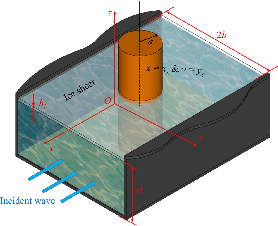
Figure 1. Coordinate system and sketch of the problem.
Based on the assumption that the fluid with density  $\rho$ is ideal, incompressible and homogeneous, and its motion is irrotational, the fluid flow can be described by the velocity potential $\varPhi$. For small amplitude waves, linearization of the boundary conditions on the ice sheet can be introduced further. For a sinusoidal wave in time with frequency $\omega$, the total velocity potential can be written in the form
 \begin{equation} \varPhi={\rm Re}\{\phi(x,y,z)\times {\rm e}^{{\rm i}\omega t}\}, \end{equation}
where  $\phi$ is composed of the incident component $\phi _I$ and diffracted component $\phi _D$. The law of conservation of mass requires $\phi$ to satisfy the Laplace equation throughout the fluid domain, which can be expressed as
 \begin{equation} \nabla^{2}\phi + \frac{\partial^{2} \phi}{\partial z^{2}}=0,\quad -\infty< x<{+}\infty,\ -b\leq y\leq b,\ -H\leq z \leq 0, \end{equation}
where  $\nabla ^{2}$ is the two-dimensional Laplacian on the $Oxy$ plane. Here, the ice sheet is modelled as a thin elastic plate. Then the boundary condition on the ice sheet can be written as
 \begin{equation} (L\nabla^{4} - m_i\omega^{2} + \rho g)\,\frac{\partial \phi}{\partial z}-\rho \omega^{2}\phi = 0,\quad z=0, \end{equation}
where  $L=Eh_i^{3}/[12(1-\nu ^{2} )]$ represents the effective flexural rigidity of the ice sheet, $E$ and $\nu$ denote its Young's modulus and Poisson's ratio, respectively, $m_i=\rho _i h_i$ represents the mass per unit area of the ice sheet, and $g$ is the acceleration due to gravity. The impermeable condition on the body surface $S_B$ can be expressed as
 \begin{equation} \frac{\partial \phi}{\partial n}=0,\quad \text{on}\ S_B, \end{equation}
where  $\boldsymbol {n}=(n_x,n_y,0)$ is the unit normal vector of $S_B$ pointing into the body. The impermeable conditions are also enforced on the rigid side walls and the bottom of the channel, i.e.
 \begin{gather} \frac{\partial \phi}{\partial y}=0,\quad y={\pm} b, \end{gather}
 \begin{gather}\frac{\partial \phi}{\partial z}=0,\quad z={-}H. \end{gather}
At far field, the radiation condition should be imposed to ensure that the disturbed wave propagates outwards. In addition to all the above, edge conditions should be imposed at the intersections of the ice sheet with the two channel walls and with the vertical cylinder. In the present work, without loss of generality, case studies are made for the clamped and free edges. The former requires zero deflection and slope at the intersection line, while the latter requires zero bending moment and Kirchhoff shear force. Following the formulas given in Timoshenko & Woinowsky-Krieger (Reference Timoshenko and Woinowsky-Krieger1959), the edge conditions at  $y=\pm b, z=0$ can be expressed as
 \begin{equation} \left.\begin{array}{c@{}} \dfrac{\partial \phi}{\partial z} = 0,\quad \dfrac{\partial^{2}\phi}{\partial y\,\partial z}=0,\quad\text{Clamped},\\[6pt] \dfrac{\partial^{3}\phi}{\partial y^{2}\,\partial z}+\nu \dfrac{\partial^{3}\phi}{\partial x^{2}\,\partial z} = 0, \quad \dfrac{\partial^{4}\phi}{\partial y^{3}\,\partial z}+(2-\nu) \dfrac{\partial^{4}\phi}{\partial x^{2}\,\partial y\,\partial z}=0,\quad\text{Free}. \end{array}\right\} \end{equation}
The edge conditions at the intersection line of the ice sheet and the surface of the vertical cylinder can be written as
 \begin{equation} \left. \begin{array}{c@{}} \dfrac{\partial \phi}{\partial z} = 0,\quad \dfrac{\partial^{2}\phi}{\partial r\,\partial z}=0,\quad\text{Clamped},\\[6pt] \mathcal{B}\left(\dfrac{\partial \phi}{\partial z}\right)=0, \quad \mathcal{S}\left(\dfrac{\partial \phi}{\partial z}\right)=0, \quad\text{Free}, \end{array}\right\} \end{equation}
where the operators  $\mathcal {B}$ and $\mathcal {S}$ are defined as
 \begin{equation} \left. \begin{array}{c@{}} \mathcal{B} = \nabla^{2} - \dfrac{1-\nu}{a}\left(\dfrac{1}{a}\,\dfrac{\partial^{2}}{\partial \theta^{2}}+\dfrac{\partial}{\partial r}\right),\\ \mathcal{S} = \dfrac{\partial}{\partial r}\nabla^{2} + \dfrac{1-\nu}{a^{2}}\left(\dfrac{\partial^{3}}{\partial r\,\partial \theta^{2}}-\dfrac{1}{a}\,\dfrac{\partial^{2}}{\partial \theta^{2}}\right), \end{array} \right\} \end{equation}
and  $(r,\theta )$ is defined in (2.1).
3. Solution procedure
3.1. Green function for a channel covered fully by an ice sheet
To solve the boundary value problem, the Green function  $G(x,y,z;x_0,y_0,z_0)$ is first derived, which is the velocity potential at point $(x,y,z)$ due to a single source at point $(x_0,y_0,z_0)$. This $G$ should satisfy the following equation in the entire fluid domain:
 \begin{equation} \nabla^{2}G + \frac{\partial^{2} G}{\partial z^{2}}=2{\rm \pi}\,\delta(x-x_0)\,\delta(y-y_0)\,\delta(z-z_0), \end{equation}
where  $\delta (\cdot )$ denotes the Dirac delta function. The same boundary conditions in (2.4), (2.6)–(2.10) and at far field also need to be satisfied by $G$. To obtain the solution, we may apply the Fourier transform along the $x$-direction,
 \begin{equation} \hat{G}=\frac{1}{2{\rm \pi}}\int_{-\infty}^{+\infty}G\, {\rm e}^{-{\rm i}kx}\,{{\rm d}\kern0.7pt x} \end{equation}
to (3.1). The governing equation becomes
 \begin{equation} -k^{2}\hat{G}+\frac{\partial^{2}\hat{G}}{\partial y^{2}}+ \frac{\partial^{2}\hat{G}}{\partial z^{2}}={\rm e}^{-{\rm i}k x_0}\,\delta(y-y_0)\,\delta(z-z_0). \end{equation}
To derive the solution of (3.3),  $\hat {G}$ can be expressed as
 \begin{equation} \hat{G} = \hat{G}_p + \hat{G}_g, \end{equation}
where  $\hat {G}_p$ is a particular solution of (3.3) satisfying conditions in (2.4) and (2.7) – or the solution corresponding to the problem in unbounded ocean with an ice cover – while $\hat {G}_g$ is a general solution of (3.3) with zero right-hand side, which is introduced to satisfy the remaining boundary conditions. Based on the procedure of Wehausen & Laitone (Reference Wehausen and Laitone1960), $\hat {G}_p$ can be derived through the Fourier transform method as
 \begin{equation} \hat{G}_p={-}\frac{{\rm e}^{{-{\rm i}}kx_0}}{2{\rm \pi}}\int_{-\infty}^{+\infty} \frac{{\rm e}^{-{\rm i}\sigma|y-y_0|}\,f(\alpha,z_>,z_<)}{\alpha\, K(\alpha,\omega)}\, {{\rm d}} \sigma, \end{equation}
where
 \begin{gather} f(\alpha,z_>,z_<)=[(L\alpha^{4}+\rho g -m_i\omega^{2})\alpha\cosh(\alpha z_>)+\rho \omega^{2}\sinh(\alpha z_>)]\cosh\alpha(z_<{+}H), \end{gather}
 \begin{gather}K(\alpha,\omega) = (L\alpha^{4} + \rho g -m_i\omega^{2})\alpha \sinh\alpha H - \rho\omega^{2}\cosh \alpha H, \end{gather}
with  $\alpha =(\sigma ^{2}+k^{2})^{1/2}$, and $z_>$ and $z_<$ are defined as $z_>=\max \{z,z_0\}$ and $z_<=\min \{z,z_0\}$. Here, we may denote the roots of $K(\alpha,\omega )=0$ as $\alpha =\pm \kappa _m$ ( $m=-2,-1,0,\ldots$), where $\kappa _0$ is the purely positive real root, $\kappa _{-2}$ and $\kappa _{-1}$ are two complex roots with positive imaginary part, and $\kappa _m$ ( $m=1,2,3,\ldots$) are an infinite number of purely positive imaginary roots. When $\kappa _0^{2}>k^{2}$, there will be singularities in the integrand of (3.5) at $\sigma =\pm (\kappa _0^{2}-k^{2})^{1/2}$. To satisfy the outgoing wave radiation condition at far field, the integration path should pass under (over) the poles at $\sigma =-(\kappa _0^{2}-k^{2})^{1/2}$ ( $\sigma =+(\kappa _0^{2}-k^{2})^{1/2}$). In fact, if we deform the integration path in (3.5) downwards into the lower half of the complex plane and use the residue theorem, then $\hat {G}_p$ can be expressed further in a form of eigenfunction series as
 \begin{equation} \hat{G}_p={\rm i}{\rm e}^{-{\rm i}kx_0}\sum_{m={-}2}^{+\infty}\frac{{\rm e}^{-{\rm i}\sigma_m|y-y_0|}\,\psi_m(z)\,\psi_m(z_0)}{2\sigma_mQ_m}, \end{equation}
where
 \begin{gather} \psi_m(z) = \frac{\cosh\kappa_m(z+H)}{\cosh\kappa_mH}, \end{gather}
 \begin{gather}Q_m = \frac{2\kappa_mH+\sinh 2\kappa_mH}{4\kappa_m\cosh^{2}\kappa_mH} +\frac{2L\kappa_m^{4}}{\rho\omega^{2}}\tanh^{2}\kappa_mH, \end{gather}
and  $\sigma _m=-\textrm {i}(k^{2}-\kappa _m^{2})^{1/2}$. The details of the derivation of (3.8) can be found in Appendix A.
The general solution  $\hat {G}_g$ can be determined through a variable separation procedure (Li et al. Reference Li, Shi and Wu2020) as
 \begin{equation} \hat{G}_g(y,z)={\rm e}^{-{\rm i}kx_0}\sum_{m={-}2}^{+\infty}\varphi_m(y)\,\psi_m(z), \end{equation}
where  $\varphi _m(y)$ is governed by
 \begin{equation} \frac{{{\rm d}}^{2}\varphi_m}{{{\rm d} y}^{2}} + \sigma_m^{2}\varphi_m = 0,\quad -b\leq y \leq b. \end{equation}
To establish the boundary conditions of  $\varphi _m(y)$, an orthogonal inner product proposed by Sahoo, Yip & Chwang (Reference Sahoo, Yip and Chwang2001) gives
 \begin{equation} \langle \psi_m,\psi_{\tilde{m}}\rangle =\int_{{-}H}^{0}\psi_m\psi_{\tilde{m}}\, {{\rm d}}z +\left.\frac{L}{\rho \omega^{2}}\left(\frac{{{\rm d}}\psi_m}{{{\rm d}}z}\, \frac{{{\rm d}}^{3}\psi_{\tilde{m}}}{{{\rm d}}z^{3}}+\frac{{{\rm d}}^{3}\psi_m}{{{\rm d}}z^{3}}\, \frac{{{\rm d}}\psi_{\tilde{m}}}{{{\rm d}}z}\right)\right|_{z=0}=\delta_{m\tilde{m}}Q_m, \end{equation}
which is used here, where  $\delta _{ij}$ denotes the Kronecker delta function. Therefore,
 \begin{align} \left.\left\langle \frac{\partial \hat{G}}{\partial y},\psi_{\tilde{m}}\right\rangle \right|_{y={\pm} b}&=\int_{{-}H}^{0}\left.\frac{\partial \hat{G}}{\partial y}\right|_{y={\pm} b}\psi_{\tilde{m}}\, {{\rm d}}z+\left.\frac{L}{\rho \omega^{2}}\left(\frac{\partial^{2}\hat{G}}{\partial y\,\partial z}\,\frac{{{\rm d}}^{3}\psi_{\tilde{m}}}{{{\rm d}}z^{3}}+\frac{\partial^{4} \hat{G}}{\partial y\, \partial z^{3}}\,\frac{{{\rm d}} \psi_{\tilde{m}}}{{{\rm d}}z}\right)\right|_{y={\pm} b,z=0}\nonumber\\ &={\rm e}^{-{\rm i}kx_0}\,Q_{\tilde{m}}\left[\left.\frac{{{\rm d}} \varphi_{\tilde{m}}}{{\rm d} y}\right|_{y={\pm} b}\pm \frac{{\rm e}^{-{\rm i}\sigma_{\tilde{m}}(b\mp y_0)}\,\psi_{\tilde{m}}(z_0)}{2Q_{\tilde{m}}}\right]. \end{align}
Applying the impermeable condition in (2.6) to (3.14), and letting
 \begin{equation} \left.\frac{\partial^{2}\hat{G}}{\partial y\,\partial z}\right|_{y={\pm} b, z=0} =\frac{{\rm e}^{-{\rm i}kx_0}(\beta_3\pm\beta_1)}{2} \quad\text{and}\quad \left.\frac{\partial^{4}\hat{G}}{\partial y\,\partial z^{3}} \right|_{y={\pm} b,z=0}=\frac{{\rm e}^{-{\rm i}kx_0}(\beta_4\pm\beta_2)}{2}, \end{equation}
where  $\beta _j$ ( $j=1,2,3,4$) are four unknown coefficients to be determined from the edge conditions on channel walls, we have
 \begin{equation} \left.\frac{{{\rm d}} \varphi_m}{{\rm d} y}\right|_{y={\pm} b}=\frac{L\kappa_m\tanh\kappa_mH}{2\rho\omega^{2}Q_m}\times [\kappa_m^{2}(\beta_3\pm\beta_1)+(\beta_4\pm\beta_2)]\mp\frac{{\rm e}^{-{\rm i}\sigma_m(b\mp y_0)}\,\psi_m(z_0)}{2Q_m}. \end{equation}
Based on (3.12) and (3.16),  $\varphi _m$ can be found as
 \begin{equation} \varphi_m(y)=\varphi_m^{(1)}(y)+\varphi_m^{(2)}(y), \end{equation}
where
 \begin{gather} \varphi_m^{(1)}(y) = \frac{\psi_m(z_0)}{Q_m}\times\left[\frac{\cos\sigma_m(y+y_0)+{\rm e}^{{-}2{\rm i}\sigma_mb}\cos\sigma_m(y-y_0)}{2\sigma_m\sin 2\sigma_mb}\right], \end{gather}
 \begin{gather}\varphi_m^{(2)}(y)=C_m\cos\sigma_my+D_m\sin\sigma_my, \end{gather}
with
 \begin{gather} C_m ={-}\frac{L}{\rho \omega^{2}}\times\frac{\tanh\kappa_mH}{Q_m\sigma_m\sin\sigma_mb}\times (\kappa_m^{3}\beta_1+\kappa_m\beta_2), \end{gather}
 \begin{gather}D_m = \frac{L}{\rho \omega^{2}}\times\frac{\tanh\kappa_mH}{Q_m\sigma_m\cos\sigma_mb}\times (\kappa_m^{3}\beta_3+\kappa_m\beta_4). \end{gather}
In fact, it can be seen from (3.18) and (3.19) that  $\varphi _m^{(1)}$ is introduced to satisfy the impermeable condition on the channel walls, while $\varphi _m^{(2)}$ is introduced for edge conditions at $y=\pm b$ & $z=0$. To obtain $\beta _j$ ( $j=1,2,3,4$), we may apply the edge conditions given in (2.8) to $\hat {G}$, and use (3.4), (3.8), (3.11) and (3.17)–(3.19). A system of linear equations of the following form can be established:
 \begin{equation} \left[ \begin{array}{cccc} A_{11} & A_{12} & A_{13} & A_{14}\\ A_{21} & A_{22} & A_{23} & A_{24}\\ A_{31} & A_{32} & A_{33} & A_{34}\\ A_{41} & A_{42} & A_{43} & A_{44}\\ \end{array} \right]\left[ \begin{array}{c} \beta_1\\ \beta_2\\ \beta_3\\ \beta_4\\ \end{array} \right]=\left[ \begin{array}{c} B_1\\ B_2\\ B_3\\ B_4\\ \end{array} \right], \end{equation}
where the expressions for elements  $A_{ij}$, $B_j$ and the solution $\beta _j$ ( $i,j=1,2,3,4$) are given in Appendix B. Substituting $\beta _j$ in (B8) and (B9) into (3.18b), and using (B1) and (B3), $\varphi _m^{(2)}$ can be written as
 \begin{align} \varphi_m^{(2)}(y)&=\sum_{m^{\prime}={-}2}^{+\infty}\frac{I_mI_{m^{\prime}}\,\psi_{m^{\prime}}(z_0)}{Q_m Q_{m^{\prime}}}\left[\frac{\cos\sigma_my \cos\sigma_{m^{\prime}}y_0}{\mathcal{F}_S (k,\omega)\sin\sigma_mb\sin\sigma_{m^{\prime}}b}\right.\nonumber\\ &\quad +\left.\frac{\sin\sigma_my \sin\sigma_{m^{\prime}}y_0}{\mathcal{F}_A(k,\omega)\cos\sigma_mb \cos\sigma_{m^{\prime}}b}\right], \end{align}
where
 \begin{gather} I_m(k)=\zeta_m(k)\times\frac{\kappa_m\tanh\kappa_mH}{\sigma_m},\end{gather}
 \begin{gather} \mathcal{F}_S(k,\omega)={-}2\sum_{m={-}2}^{+\infty}\frac{\kappa_m^{2} \tanh^{2}\kappa_mH}{Q_m\sigma_m}\times\frac{\zeta_m^{2}(k)}{\tan\sigma_mb}, \end{gather}
 \begin{gather}\mathcal{F}_A(k,\omega)=2\sum_{m={-}2}^{+\infty}\frac{\kappa_m^{2} \tanh^{2}\kappa_mH}{Q_m\sigma_m}\times\frac{\zeta_m^{2}(k)}{\cot\sigma_mb} \end{gather}
and
 \begin{equation} \zeta_m(k)=\left\{ \begin{array}{@{}ll} 1, & \text{clamped-clamped},\\[3pt] \sigma_m^{2}(k)+\nu k^{2}, & \text{free-free}.\\ \end{array}\right. \end{equation}
Once  $\hat {G}_p$ and $\hat {G}_g$ are found, the Green function $G$ can be obtained by performing the inverse Fourier transform. Using (e.g. Linton et al. Reference Linton, Evans and Smith1992)
 \begin{equation} \int_{-\infty}^{+\infty}\frac{{\rm e}^{{\rm i}k(x-x_0)-{\rm i} \sigma_m|y-y_0|}}{\sigma_m}\, {{\rm d}}k={-}{\rm \pi}\mathscr{H}_0^{(1)}(\kappa_mR), \end{equation}
where  $R = [(x-x_0)^{2}+(y-y_0)^{2}]^{1/2}$ and $\mathscr {H}_n^{(1)}$ denotes the $n$th-order Hankel function of the first kind, we have the Green function
 \begin{align} &G(x,y,z;x_0,y_0,z_0)={-}\frac{{\rm i}{\rm \pi}}{2}\sum_{m={-}2}^{+\infty} \frac{\psi_m(z)\,\psi_m(z_0)}{Q_m}\,\mathscr{H}_0^{(1)}(\kappa_mR)\nonumber\\ &\quad +\sum_{m={-}2}^{+\infty}\frac{\psi_m(z)\,\psi_m(z_0)}{Q_m} \int_{0}^{+\infty}\left[\frac{\cos\sigma_m(y+y_0)+{\rm e}^{{-}2{\rm i} \sigma_mb}\cos\sigma_m(y-y_0)}{\sigma_m\sin 2\sigma_mb}\right] \cos k(x-x_0)\, {{\rm d}}k\nonumber\\ &\quad +\sum_{m={-}2}^{+\infty}\sum_{m^{\prime}={-}2}^{+\infty} \frac{2\psi_m(z)\,\psi_{m^{\prime}}(z_0)}{Q_mQ_{m^{\prime}}} \int_{\mathscr{L}}I_mI_{m^{\prime}}\left[ \begin{aligned} & \frac{\cos\sigma_my \cos\sigma_{m^{\prime}}y_0}{\mathcal{F}_S(k, \omega)\sin\sigma_mb\sin\sigma_{m^{\prime}}b}\\ & \quad +\frac{\sin\sigma_my \sin\sigma_{m^{\prime}}y_0}{\mathcal{F}_A (k,\omega)\cos\sigma_mb\cos\sigma_{m^{\prime}}b} \end{aligned} \right]\cos k(x-x_0)\, {{\rm d}}k. \end{align}
In (3.26), there will be singularities in the integrand when  $\mathcal {F}_S (k_j,\omega )=0$ or $\mathcal {F}_A (k_j,\omega )=0$ ( $j=1,2,\ldots,N_s$), where $k_j$ denotes all the corresponding purely positive real roots with $k_1< k_2< \cdots < k_{N_s}$, and $N_s$ is the number of roots. To satisfy the radiation condition at far field, which requires the disturbed waves to propagate away from the source, the integration path $\mathscr {L}$ in (3.26) from $0$ to $+\infty$ should pass over all the poles at $k_j$. In fact, $\mathcal {F}_S (k,\omega )\times \mathcal {F}_A (k,\omega )=0$ corresponds to the dispersion equation (Ren et al. Reference Ren, Wu and Li2020), or relationship between wavenumber and frequency for the propagating wave in the channel. Furthermore, it can be observed (3.26) that $\mathcal {F}_S(k,\omega )$ is combined with $\cos \sigma _my$, which means that $\mathcal {F}_S(k_j,\omega )$ corresponds to a symmetric progressing wave about $y=0$ with wavenumber $k_j$, while $\mathcal {F}_A(k,\omega )$ with $\sin \sigma _my$ corresponds to antisymmetric waves.
3.2. The velocity potential of the incident wave
For the problems in the free surface channel, one form of the incident wave could be assumed as two-dimensional along the channel length and has no transverse variation. However, in the ice-covered channel, such a form is not possible due to the physical constraints at the ice sheet edges. The propagating wave will be always three-dimensional (Ren et al. Reference Ren, Wu and Li2020), and there is always variation in the transverse direction. In fact, there are an infinite number of modes in the  $y$-direction, and all these modes are coupled. Here, when the edge conditions on channel walls are the same, we may consider an incident wave symmetric about $y=0$. Following a similar procedure for solving the Green function shown above, $\phi _I$ can be obtained by finding the non-trivial solution of the homogeneous problem, which provides
 \begin{equation} \phi_I={-}{\rm i}\,\frac{Ag}{\omega\,\chi(\lambda)}\times {\rm e}^{{\rm i}\lambda (x-x_c)}\times\sum_{m={-}2}^{+\infty}\frac{I_m(\lambda)\, \psi_m(z)}{Q_m}\,\frac{\cos[\sigma_m(\lambda)\,y]}{\sin[\sigma_m(\lambda)\,b]}, \end{equation}
where  $A$ is a parameter related to the amplitude of the incident wave, $\sigma _m(\lambda )=-\textrm {i}(\lambda ^{2}-\kappa _m^{2})^{1/2}$, $\lambda$ is the wavenumber along the $x$-direction, or the solution of the dispersion equation which also requires $\mathcal {F}_S(\lambda,\omega )=0$. Similar to the problem in the free surface channel, $\lambda$ is taken as the largest positive real root here, or $\lambda =k_{N_s}$. Now, $\chi (\lambda )$ in (3.27) can be expressed as
 \begin{equation} \chi(\lambda)=\frac{1}{\kappa_0\tanh\kappa_0 H}\sum_{m={-}2}^{+\infty} \frac{I_m(\lambda)\,\kappa_m\tanh\kappa_mH}{Q_m\sin[\sigma_m(\lambda)\,b]}. \end{equation}
The ice sheet deflection due to the incident wave can be obtained from  $\eta _I=-({\textrm {i}}/{\omega })({\partial \phi _I}/{\partial z})|_{z=0}$. Then, on $y=0$, we have
 \begin{equation} \eta_I(x,0)={-}\frac{Ag}{\omega}\times\kappa_0\tanh\kappa_0H \times {\rm e}^{{\rm i}\lambda(x-x_c)}. \end{equation}
It is interesting to see that along the centre line of the tank, the expression for the incident wave is similar to that in unbounded ocean given in Ren et al. (Reference Ren, Wu and Ji2018b).
3.3. Solution through the source distribution method
Once the Green function is derived, the velocity potential can be determined from a boundary integral equation. For the problem of wave diffraction by a vertical cylinder in a free surface channel, the boundary integral equation can be established directly through distributing sources over the body surface (e.g. Linton et al. Reference Linton, Evans and Smith1992). However, when there is an ice sheet, the integral equation has to be re-derived, and the edge conditions must be imposed. The detailed derivation is given in Appendix C. In the result, there is an extra line integral along the edge  $\mathcal {L}$ between the body surface and the ice sheet (see (C3)), which contains terms ${\partial ^{4}\phi _D}/{\partial n\,\partial z^{3}}$ and ${\partial ^{2}\phi _D}/{\partial n\,\partial z}$. This is similar to that in Ren et al. (Reference Ren, Wu and Ji2018a); however, their procedure becomes difficult here due to the presence of the channel walls, therefore a different one is introduced here. From the derivation given in Appendix C, using (C9) and the symmetric property of the Green function, or $G(x,y,z;x_0,y_0,z_0 )=G(x_0,y_0,z_0;x,y,z)$, we have
 \begin{equation} \phi_D(x,y,z)=a\oint_{\mathcal{L}}\langle G(x,y,z;x_0,y_0,z_0), \varPsi(x_0,y_0,z_0)\rangle \, {{\rm d}} \theta_0. \end{equation}
where  $x_0-x_c=a\sin \theta _0$ and $y_0-y_c=a\cos \theta _0$, the operator $\langle \ \rangle$ is defined in (3.13), and $\varPsi$ is the strength of the source distributed on the body surface. To obtain $\phi _D$, we may expand $\varPsi$ into a double series as
 \begin{equation} \varPsi(a,\theta_0,z_0)=\frac{1}{2{\rm \pi} a}\sum_{n={-}\infty}^{+\infty}\sum_{m={-}2}^{+\infty} \frac{b_{n,m}}{Q_m\,\mathcal{J}_n(\kappa_ma)}\times\psi_m(z_0)\, {\rm e}^{-{\rm i}n\theta_0}, \end{equation}
where  $b_{n,m}$ are unknown coefficients, and $\mathcal {J}_n$ denotes the $n$th-order Bessel function of the first kind. The Green function can also be expressed in the cylindrical coordinate system. Similar to Wu (Reference Wu1998), we may define
 \begin{equation} k = \kappa_m\cos\gamma_m\quad \text{and}\quad \sigma_m=\kappa_m\sin\gamma_m. \end{equation}
Using the two identities (Abramowitz & Stegun Reference Abramowitz and Stegun1970)
 \begin{gather} \mathscr{H}_0^{(1)}(\kappa_mR)=\sum_{n={-}\infty}^{+\infty} \mathscr{H}_n^{(1)}(\kappa_mr)\,\mathcal{J}_n(\kappa_ma)\, {\rm e}^{{\rm i}n(\theta_0-\theta)}, \end{gather}
 \begin{gather}{\rm e}^{{\rm i}[k(x-x_c)\pm\sigma_m(y-y_c)]}=\sum_{n={-}\infty}^{+\infty}\mathcal{J}_n(\kappa_mr)\, {\rm e}^{{\rm i}n(\theta\pm\gamma_m)}, \end{gather}
(3.26) can be transferred to coordinates  $(r,\theta,z)$ and $(a,\theta _0,z_0 )$ as
 \begin{align} &G(r,\theta,z;a,\theta_0,z_0)={-}\frac{{\rm i}{\rm \pi}}{2}\sum_{n={-}\infty}^{n={+}\infty}\sum_{m={-}2}^{+\infty} \frac{\psi_m(z)\,\psi_m(z_0)}{Q_m}\,\mathscr{H}_n^{(1)}(\kappa_mr)\, \mathcal{J}_n(\kappa_ma)\, {\rm e}^{{\rm i}n(\theta_0-\theta)}\nonumber\\ &\quad +\sum_{n={-}\infty}^{+\infty}\sum_{n^{\prime}={-}\infty}^{+\infty}\sum_{m={-}2}^{+\infty} \mathcal{C}_{n,n^{\prime},m}\,\psi_m(z)\,\psi_m(z_0)\,\mathcal{J}_{n^{\prime}}(\kappa_mr)\, \mathcal{J}_n(\kappa_ma)\, {\rm e}^{{\rm i}(n^{\prime}\theta+n\theta_0)}\nonumber\\ &\quad +\sum_{n={-}\infty}^{+\infty}\sum_{n^{\prime}={-}\infty}^{+\infty}\sum_{m={-}2}^{+\infty} \sum_{m^{\prime}={-}2}^{+\infty}\mathcal{D}_{n,n^{\prime},m,m^{\prime}}\,\psi_{m^{\prime}}(z)\, \psi_m(z_0)\,\mathcal{J}_{n^{\prime}}(\kappa_{m^{\prime}}r)\,\mathcal{J}_n(\kappa_ma)\, {\rm e}^{{\rm i}(n^{\prime}\theta+n\theta_0)}, \end{align}
where
 \begin{gather} \mathcal{C}_{n,n^{\prime},m}=\frac{1}{Q_m}\int_{0}^{+\infty} \frac{G_{n,n^{\prime},m}+G_{n^{\prime},n,m}}{2\sigma_m\sin 2\sigma_mb}\, {{\rm d}}k, \end{gather}
 \begin{gather}\mathcal{D}_{n,n^{\prime},m,m^{\prime}}=\frac{1}{Q_mQ_{m^{\prime}}} \int_{\mathscr{L}}I_mI_{m^{\prime}}\left[ \begin{aligned} & \frac{({-}1)^{n^{\prime}}E_{n,m}E_{{-}n^{\prime},m^{\prime}}+({-}1)^{n} E_{{-}n,m}E_{n^{\prime},m^{\prime}}}{\mathcal{F}_S(k,\omega)\sin \sigma_mb\sin\sigma_{m^{\prime}}b}\\ & \quad +\frac{({-}1)^{n^{\prime}}F_{n,m}F_{{-}n^{\prime},m^{\prime}} +({-}1)^{n}F_{{-}n,m}F_{n^{\prime},m^{\prime}}}{\mathcal{F}_A(k,\omega) \cos\sigma_mb\cos\sigma_{m^{\prime}}b} \end{aligned} \right] {{\rm d}}k, \end{gather}
with
 \begin{gather} G_{n,n^{\prime},m}(k)=({-}1)^{n^{\prime}}\cos [2\sigma_my_c+(n-n^{\prime})\gamma_m]+{\rm e}^{{-}2{\rm i}\sigma_mb}({-}1)^{n^{\prime}}\cos(n+n^{\prime})\gamma_m, \end{gather}
 \begin{gather}E_{n,m}(k) = \cos(\sigma_my_c+n\gamma_m), \end{gather}
 \begin{gather}F_{n,m}(k)=\sin(\sigma_my_c+n\gamma_m). \end{gather}
Substituting (3.31) and (3.34) into (3.30), we obtain
 \begin{align} \phi_D(r,\theta,z)&={-}\frac{{\rm i}{\rm \pi}}{2}\sum_{n={-}\infty}^{+\infty} \sum_{m={-}2}^{+\infty}\frac{b_{n,m}}{Q_m}\,\mathscr{H}_n^{(1)}(\kappa_mr)\, \psi_m(z)\, {\rm e}^{-{\rm i}n\theta}\nonumber\\ &\quad +\sum_{n={-}\infty}^{+\infty}\sum_{n^{\prime}={-}\infty}^{+\infty} \sum_{m={-}2}^{+\infty}b_{n,m}\,\mathcal{C}_{n,n^{\prime},m}\, \mathcal{J}_{n^{\prime}}(\kappa_mr)\,\psi_m(z)\, {\rm e}^{{\rm i}n^{\prime}\theta}\nonumber\\ &\quad +\sum_{n={-}\infty}^{+\infty}\sum_{n^{\prime}={-}\infty}^{+\infty} \sum_{m={-}2}^{+\infty}\sum_{m^{\prime}={-}2}^{+\infty}b_{n,m}\, \mathcal{D}_{n,n^{\prime},m,m^{\prime}}\,\mathcal{J}_{n^{\prime}} (\kappa_{m^{\prime}}r)\,\psi_{m^{\prime}}(z)\, {\rm e}^{{\rm i}n^{\prime}\theta}. \end{align}
Similarly,  $\phi _I$ can be expressed in the cylindrical coordinate system by applying (3.33b)–(3.27). This gives
 \begin{equation} \phi_I(r,\theta,z)={-}\frac{{\rm i}Ag}{\omega\,\chi(\lambda)} \sum_{n={-}\infty}^{+\infty}\sum_{m={-}2}^{+\infty}\frac{I_m(\lambda)\, E_{n,m}(\lambda)}{Q_m\sin[\sigma_m(\lambda)\,b]}\,\mathcal{J}_n(\kappa_mr)\, \psi_m(z)\, {\rm e}^{{\rm i}n\theta}. \end{equation}
To obtain  $b_{n,m}$, applying the inner product in (3.13) to $\partial \phi /\partial r$ and $\psi _{\tilde {m}}$ on $r=a$, we have
 \begin{equation} \left.\left\langle \frac{\partial \phi}{\partial r},\psi_{\tilde{m}}\right\rangle \right|_{r=a}=\int_{{-}H}^{0}\left.\left\langle \frac{\partial \phi}{\partial r} \psi_{\tilde{m}}\right\rangle \right|_{r=a}\, {{\rm d}}z+\frac{L}{\rho \omega^{2}} \left.\left(\frac{\partial^{2}\phi}{\partial r\,\partial z}\, \frac{{{\rm d}}^{3}\psi_{\tilde{m}}}{{{\rm d}}z^{3}}+\frac{\partial^{4}\phi}{\partial r\,\partial z^{3}}\,\frac{{{\rm d}} \psi_{\tilde{m}}}{{{\rm d}}z}\right)\right|_{r=a,z=0}. \end{equation}
Substituting the impermeable condition on  $r=a$ (2.5) into (3.39) and letting
 \begin{equation} \left.\frac{\partial^{2}\phi}{\partial r\,\partial z}\right|_{r=a,z=0} ={-}\sum_{n={-}\infty}^{+\infty}c_n\,{\rm e}^{{\rm i}n\theta} \quad\text{and}\quad\left.\frac{\partial^{4}\phi}{\partial r\, \partial z^{3}}\right|_{r=a,z=0}={-}\sum_{n={-}\infty}^{+\infty}d_n\,{\rm e}^{{\rm i} n\theta}, \end{equation}
a system of linear equations of the following form can be obtained:
 \begin{align} &\frac{{\rm i}{\rm \pi}}{2}\,\frac{({-}1)^{n+1}\mathscr{H}_n^{(1){\prime}} (\kappa_ma)}{Q_m\,\mathcal{J}_n^{\prime}(\kappa_ma)}\, b_{{-}n,m}+\sum_{n^{\prime}={-}\infty}^{+\infty}\mathcal{C}_{n^{\prime}, n,m}\,b_{n^{\prime},m}+\sum_{n^{\prime}={-}\infty}^{+\infty} \sum_{m^{\prime}={-}2}^{+\infty}\mathcal{D}_{n^{\prime},n,m^{\prime},m}\, b_{n^{\prime},m^{\prime}}\nonumber\\ &\quad +\frac{L\tanh\kappa_mH}{\rho\omega^{2}Q_m\,\mathcal{J}_n^{\prime} (\kappa_ma)}\,(\kappa_m^{2}c_n+d_n)=\frac{{\rm i}Ag}{\omega\,\chi(\lambda)}\, \frac{I_m(\lambda)\,E_{n,m}(\lambda)}{Q_m\sin[\sigma_m(\lambda)\,b]}, \end{align}
where  $-\infty < n<+\infty$ and $-2\leq m <+\infty$, and $\mathscr {H}_n^{(1)\prime }(z)$ and $\mathcal {J}_n^{\prime }(z)$ denote the derivatives of $\mathscr {H}_n^{(1)}(z)$ and $\mathcal {J}_n(z)$, respectively. In addition to the imposed impermeable condition on the body surface, the edge conditions also need to be applied to $\phi$. Here, we may give an example of the clamped edge at the intersection line of the ice sheet and the body surface $\mathcal {L}$, and other conditions can be treated in a similar way. Substituting (3.37) and (3.38) into (2.9), the condition of zero deflection provides
 \begin{align} &\frac{{\rm i}{\rm \pi}}{2}\sum_{m={-}2}^{+\infty}\frac{({-}1)^{n+1} \mathscr{H}_n^{(1)}(\kappa_ma)\,\kappa_m\tanh\kappa_mH}{Q_m}\,b_{{-}n,m}\nonumber\\ &\qquad +\sum_{n^{\prime}={-}\infty}^{+\infty}\sum_{m={-}2}^{+\infty} \mathcal{C}_{n^{\prime},n,m}\,\mathcal{J}_n(\kappa_ma)\,b_{n^{\prime},m} \kappa_m\tanh\kappa_mH\nonumber\\ &\qquad +\sum_{n^{\prime}={-}\infty}^{+\infty}\sum_{m={-}2}^{+\infty} \sum_{m^{\prime}={-}2}^{+\infty}\mathcal{D}_{n^{\prime},n,m^{\prime},m}\, \mathcal{J}_n(\kappa_ma)\,b_{n^{\prime},m^{\prime}}\kappa_m\tanh\kappa_mH\nonumber\\ &\quad=\frac{{\rm i}Ag}{\omega\,\chi(\lambda)}\sum_{m={-}2}^{+\infty} \frac{I_m(\lambda)\,E_{n,m}(\lambda)\,\mathcal{J}_n(\kappa_ma)\, \kappa_m\tanh\kappa_mH}{Q_m\sin[\sigma_m(\lambda)\,b]},\quad -\infty< n<{+}\infty. \end{align}
The condition of zero slope gives
 \begin{equation} c_n = 0,\quad -\infty< n<{+}\infty. \end{equation}
In the numerical computation, the infinite series in (3.41) and (3.42) are truncated at  $n=\pm N$ and $m=M$, respectively. We have $(2N+1)(M+5)$ unknowns in total, $(2N+1)(M+3)$ of which are $b_{n,m}$, and $(2N+1)$ are $c_n$ and $d_n$. From (3.41), we obtain $(2N+1)(M+3)$ equations, while (3.42) and (3.43) provide an additional $2\times (2N+1)$ equations. Thus there is a total of $(2N+1)(M+5)$ equations, which is the same as the number of unknowns.
After the coefficients  $b_{n,m}$, $c_n$ and $d_n$ are found, substituting (3.41) into (3.37) and (3.38), the total velocity potential $\phi$ can be further expressed as
 \begin{align} \phi(r,\theta,z)&={-}\frac{{\rm i}{\rm \pi}}{2}\sum_{n={-}\infty}^{+\infty} \sum_{m={-}2}^{+\infty}\frac{b_{n,m}}{Q_m}\left[\frac{\mathscr{H}_n^{(1)} (\kappa_mr)}{\mathcal{J}_n(\kappa_mr)}-\frac{\mathscr{H}_n^{(1)\prime} (\kappa_ma)}{\mathcal{J}_n^{\prime}(\kappa_ma)}\right]\mathcal{J}_n(\kappa_mr)\, \psi_m(z)\, {\rm e}^{-{\rm i}n\theta}\nonumber\\ &\quad -\frac{L}{\rho \omega^{2}}\sum_{n={-}\infty}^{+\infty} \sum_{m={-}2}^{+\infty}\frac{(\kappa_m^{2}c_n +d_n)\tanh\kappa_mH}{Q_m}\, \frac{\mathcal{J}_n(\kappa_mr)}{\mathcal{J}_n^{\prime}(\kappa_ma)}\, \psi_m(z)\, {\rm e}^{{\rm i}n\theta}. \end{align}
3.4. Hydrodynamic forces and vertical shear forces on the vertical cylinder
Once the velocity potential is found, the hydrodynamic forces on the vertical cylinder can be obtained through the integration of hydrodynamic pressure over the body surface, which can be expressed as
 \begin{equation} F_j={\rm i}\omega\rho\iint_{S_B}\phi n_j\, {{\rm d}}S,\quad j=1,2,3,4, \end{equation}
where  $j=1,2$ correspond to the forces $F_x$ and $F_y$, and $j=3,4$ correspond to the moments $M_x$ and $M_y$ about the bottom of the channel on $z=-H$; also, $(n_1,n_2,n_3,n_4 )=(n_x,n_y,-(z+H)n_y,(z+H)n_x )$. For the present case of a vertical circular cylinder, we have $n_x=-\sin \theta =-(\textrm {e}^{\textrm {i}\theta }-\textrm {e}^{-\textrm {i}\theta })/2\textrm {i}$ and ${n_y=-\cos \theta =-(\textrm {e}^{\textrm {i}\theta }+\textrm {e}^{-\textrm {i}\theta })/2}$. Substituting these and (3.44) into (3.45), we obtain
 \begin{align} &\left[ \begin{array}{c} F_x \\ F_y \\ \end{array} \right]={\rm \pi}\omega\rho a\times\left[ \begin{array}{cc} 1 & -1\\ {\rm i} & {\rm i}\\ \end{array} \right]\nonumber\\ &\quad \times\left\{ \begin{aligned} & \frac{1}{a}\sum_{m={-}2}^{+\infty}\frac{\tanh\kappa_mH}{\kappa_m^{2} Q_m\,\mathcal{J}_{1}^{\prime}(\kappa_ma)}\times\left[ \begin{array}{c} b_{1,m} \\ -b_{{-}1,m}\\ \end{array} \right]\\ & \quad +\frac{L}{\rho\omega^{2}}\sum_{m={-}2}^{+\infty} \frac{\mathcal{J}_1(\kappa_ma)\tanh^{2}\kappa_mH}{\kappa_mQ_m\,\mathcal{J}_1^{\prime} (\kappa_ma)}\times\left[ \begin{array}{c} \kappa_m^{2}c_{{-}1} + d_{{-}1}\\ \kappa_m^{2}c_1 + d_1\\ \end{array} \right] \end{aligned} \right\}, \end{align}
 \begin{align} &\left[ \begin{array}{c} M_x \\ M_y \\ \end{array} \right]={-}{\rm \pi}\omega\rho a\times\left[ \begin{array}{cc} {\rm i} & {\rm i}\\ -1 & 1\\ \end{array} \right]\nonumber\\ &\quad \times\left\{ \begin{aligned} & \frac{1}{a}\sum_{m={-}2}^{+\infty}\frac{\kappa_mH\sinh\kappa_mH -\cosh\kappa_mH+1}{\mathcal{J}_{1}^{\prime}(\kappa_ma)\, \kappa_m^{3}Q_m\cosh\kappa_mH}\times\left[ \begin{array}{c} b_{1,m} \\ -b_{{-}1,m}\\ \end{array} \right]\\ & \quad +\frac{L}{\rho\omega^{2}}\sum_{m={-}2}^{+\infty} \frac{\mathcal{J}_1(\kappa_ma)\,(\kappa_mH\sinh\kappa_mH- \cosh\kappa_mH\!+\!1)}{\mathcal{J}_1^{\prime}(\kappa_ma)\, \kappa_m^{2}Q_m\cosh\kappa_mH\coth\kappa_mH}\times\left[ \begin{array}{@{}c@{}} \kappa_m^{2}c_{{-}1} \!+\! d_{{-}1}\\ \kappa_m^{2}c_1 \!+\! d_1\\ \end{array} \right] \end{aligned} \right\}. \end{align}
When the ice sheet is clamped to the surface of the cylinder, there will be a vertical shear force on the body. The total vertical shear force  $V$ can be obtained from
 \begin{equation} V = \int_{0}^{2{\rm \pi}}\tau(\theta)\,a\, {{\rm d}} \theta, \end{equation}
where  $\tau (\theta )$ is the shear stress distribution along the intersection line, which can be expressed as (Ugural Reference Ugural1999)
 \begin{equation} \tau(\theta)={-}{\rm i}\,\frac{L}{\omega}\,\frac{\partial }{\partial r} \left.\left(\nabla^{2}\frac{\partial \phi}{\partial z}\right) \right|_{r=a,z=0}={\rm i}\,\frac{L}{\omega}\left.\frac{\partial^{4}\phi}{\partial r\,\partial z^{3}}\right|_{r=a,z=0}={-}{\rm i}\,\frac{L}{\omega}\sum_{n={-}\infty}^{+\infty}d_n\,{\rm e}^{{\rm i}n\theta}. \end{equation}
Substituting (3.48) into (3.47), we have
 \begin{equation} V ={-}{\rm i}\,\frac{2{\rm \pi} aL}{\omega}\,d_0. \end{equation}
3.5. Behaviour of the solution at the natural frequencies
For a given  $\omega$, the residual in (3.26) at a singularity $\mathcal {F}_S(k,\omega )=0$ ( $\mathcal {F}_A(k,\omega )=0$) can be obtained from the standard method in complex analysis. The result contains $\mathcal {F}_S^{\prime }(k,\omega )=0$ ( $\mathcal {F}_A^{\prime }(k,\omega )=0$) in the denominator, where the prime represents the derivative with respect to $k$. At some $\omega$, $\mathcal {F}_S^{\prime }(k,\omega )$ ( $\mathcal {F}_A^{\prime }(k,\omega$)) is also equal to zero when $\mathcal {F}_S(k,\omega )=0$ ( $\mathcal {F}_A(k,\omega )=0$), and then the Green function $G$ will be infinite. Physically, $\omega$ in this case is the natural frequency of the ice-covered channel. In fact, from (3.23), $k=0$ is always the solution of $\mathcal {F}_S^{\prime }(k,\omega )=0$ ( $\mathcal {F}_A^{\prime }(k,\omega )=0$). At a given $\omega$, if we further have $\mathcal {F}_S^{\prime }(k,\omega )=0$ ( $\mathcal {F}_A^{\prime }(k,\omega )=0$), then this $\omega$ will be a natural frequency. This is similar to $\kappa _0=\textrm {i}{\rm \pi} /2b$ and $\omega =[({\textrm {i}{\rm \pi} }/{2b})\tanh ({\textrm {i}{\rm \pi} H}/{2b})]^{1/2}$ ( $i=1,2,\ldots$) in the free surface channel (Linton et al. Reference Linton, Evans and Smith1992; Wu Reference Wu1998). The ice-covered channel also has an infinite number of natural frequencies, which are denoted as $\omega _c^{(i)}$ ( $i=1,2,\ldots$) here, with $\omega _c^{(1)}<\omega _c^{(2)}<\omega _c^{(3)}<\cdots$ In particular, even $i$ corresponds to $\mathcal {F}_S(0,\omega _c^{(i)})=0$, while odd $i$ corresponds to $\mathcal {F}_A(0,\omega _c^{(i)})=0$. The results near the natural frequencies can change rapidly. Here, we will show that even though the Green function is infinite at one of the natural frequencies, the velocity potential $\phi$ and hydrodynamic force may remain finite. We may consider the even modes $2i$ as an example, and the odd modes $2i-1$ can be done in a similar way. When $\omega \to \omega _c^{(2i)}$, $\mathcal {F}_S(k,\omega )$ at $k\to 0$ can be expressed asymptotically as
 \begin{equation} \mathcal{F}_S(k,\omega)\to\mathcal{F}_{S,asy}(k,\omega) =\mathcal{F}_S(0,\omega)+\tfrac{1}{2}\mathcal{F}_S^{\prime \prime}(0,\omega){\rm i}k^{2},\quad k\to 0, \end{equation}
where  $\mathcal {F}_S(0,\omega )\to 0^{\pm }$ when $\omega \to \omega _c^{(2i)}+0^{\pm }$, and $\mathcal {F}_S^{\prime \prime }(0,\omega )<0$, which can be confirmed from (3.23a). For the integrand as $\mathcal {G}(k)/\mathcal {F}_S(k,\omega )$ in (3.35b), we may re-express it as $[\mathcal {G}(k)/\mathcal {F}_S(k,\omega )- \mathcal {G}(0)/\mathcal {F}_{S,asy}(k,\omega )]+\mathcal {G}(0)/\mathcal {F}_{S,asy}(k,\omega )$. Then the first term is non-singular, and the second term can be integrated explicitly. Also, $\mathcal {D}_{n,n^{\prime },m,m^{\prime }}$ in $G$ can be written as
 \begin{equation} \mathcal{D}_{n,n^{\prime},m,m^{\prime}}=\frac{2{\rm \pi}}{\varDelta}\, \frac{I_m(0)\,I_{m^{\prime}}(0)\,E_{n,m}(0)\,E_{n^{\prime},m^{\prime}} (0)}{Q_mQ_{m^{\prime}}\sin\kappa_mb\sin\kappa_{m^{\prime}}b} +\tilde{\mathcal{D}}_{n,n^{\prime},m,m^{\prime}}+O(\varDelta), \quad\varDelta\to 0, \end{equation}
where  $\varDelta =\mu \times |2\mathcal {F}_S^{\prime \prime }(0,\omega )\,\mathcal {F}_S(0,\omega )|$, and $\mu$ is a constant depending on whether $\omega _c^{(2i)}$ is approached from the left- or right-hand side. When $\omega \to \omega _c^{(2i)}+0^{-}$, $\mu =1$ and the singular term in $\mathcal {D}_{n,n^{\prime },m,m^{\prime }}$ is from the principal value integration. When $\omega \to \omega _c^{(2i)}+0^{+}$, $\mu =-\textrm {i}$ and the singular term is from the residue term. Also, $\tilde {\mathcal {D}}_{n,n^{\prime },m,m^{\prime }}\sim O(1)$ in (3.51) is the leading term of the remaining regular part of the Green function. To analyse the behaviour of the velocity potential $\varphi$ at natural frequencies, we may employ a procedure similar to that used by Liu & Yue (Reference Liu and Yue1993) for the forward speed problem in free surface flow. Substituting (3.51) into (3.41) and rearranging the equation, we obtain
 \begin{equation} b_{{-}n,m}+\frac{4{\rm i}}{\varDelta}\times\varLambda \times\frac{({-}1)^{n}\mathcal{J}_n^{\prime}(\kappa_ma)\,I_m(0)\, E_{n,m}(0)}{\mathscr{H}_n^{(1)\prime}(\kappa_ma)\sin\kappa_mb}=\xi_{n,m}+O(\varDelta), \end{equation}
where
 \begin{gather} \varLambda=\sum_{n^{\prime}={-}\infty}^{+\infty}\sum_{m^{\prime} ={-}2}^{+\infty}\frac{I_{m^{\prime}}(0)\,E_{n^{\prime},m^{\prime}} (0)}{Q_{m^{\prime}}\sin\kappa_{m^{\prime}}b}\,b_{n^{\prime},m^{\prime}}, \end{gather}
 \begin{gather}\xi_{n,m}=\frac{2{\rm i}({-}1)^{n}\mathcal{J}_n^{\prime}(\kappa_ma)}{{\rm \pi}\, \mathscr{H}_n^{(1)\prime}(\kappa_ma)}\times\!\left[ \begin{aligned} & \frac{{\rm i}Ag}{\omega\,\chi(\lambda)}\,\frac{I_m(\lambda)\,E_{n,m}(\lambda)}{Q_m \sin[\sigma_m(\lambda)\,b]}-\sum_{n^{\prime}={-}\infty}^{+\infty} \mathcal{C}_{n^{\prime},n,m}\,b_{n^{\prime},m}\\ & \quad -\sum_{n^{\prime}={-}\infty}^{+\infty}\sum_{m^{\prime}={-}2}^{+\infty} \tilde{\mathcal{D}}_{n,n^{\prime},m,m^{\prime}}\,b_{n^{\prime},m^{\prime}} +\!\frac{L\tanh\kappa_mH}{\rho\omega^{2}Q_m\,\mathcal{J}_n^{\prime}(\kappa_ma)}\,d_n \end{aligned} \right]. \end{gather}
In (3.52),  $c_n=0$ in (3.43). Multiplying (3.41) by $\kappa _m\tanh \kappa _mH$, taking summation with respect to $m$ from $-2$ to $+\infty$, and subtracting (3.42) from the result, $d_n$ can be further expressed using $b_{n,m}$ as
 \begin{equation} d_n={-}\frac{\rho\omega^{2}}{La}\times\frac{\displaystyle\sum_{m={-}2}^{+\infty}\frac{\tanh\kappa_mH}{Q_m} \times\frac{b_{{-}n,m}}{\mathcal{J}_{{-}n}^{\prime}(\kappa_ma)}}{\displaystyle\sum_{m={-}2}^{+\infty} \frac{\kappa_m\tanh^{2}\kappa_mH}{Q_m}\times\frac{\mathcal{J}_n (\kappa_ma)}{\mathcal{J}_{n^{\prime}}(\kappa_ma)}}, \end{equation}
which indicates that  $d_n$ has the same magnitude as $b_{n,m}$. Substituting (3.52) into (3.53), $\varLambda$ can be represented as
 \begin{equation} \varLambda=\frac{\varDelta}{\varDelta+4\varGamma {\rm i}} \times\sum_{n^{\prime}={-}\infty}^{+\infty}\sum_{m^{\prime}={-}2}^{+\infty} \frac{({-}1)^{n^{\prime}}I_{m^{\prime}}(0)\,E_{n^{\prime},m^{\prime}} (0)}{Q_{m^{\prime}}\sin\kappa_{m^{\prime}}b}\,\xi_{n^{\prime},m^{\prime}}+O(\varDelta^{2}), \end{equation}
where
 \begin{equation} \varGamma=\sum_{n={-}\infty}^{+\infty}\sum_{m={-}2}^{+\infty} \frac{I_m^{2}(0)\,E_{n,m}^{2}(0)}{Q_m\sin^{2}\kappa_mb}\times \frac{\mathcal{J}_n^{\prime}(\kappa_ma)}{\mathscr{H}_n^{(1)\prime}(\kappa_ma)}. \end{equation}
At the natural frequency, we will first check whether  $\varGamma =0$. When $\varGamma \neq 0$, we may substitute (3.57) back into (3.52) and let $\varDelta =0$, then a modified matrix equation can be obtained as
 \begin{equation} b_{{-}n,m}\!+\!\frac{1}{\varGamma}\,\frac{({-}1)^{n}\mathcal{J}_n^{\prime}(\kappa_ma)\, I_m(0)\,E_{n,m}(0)}{\mathscr{H}_n^{(1)\prime}(\kappa_ma)\sin\kappa_mb} \sum_{n^{\prime}={-}\infty}^{+\infty}\sum_{m^{\prime}={-}2}^{+\infty} \frac{({-}1)^{n^{\prime}}I_{m^{\prime}}(0)\,E_{n^{\prime},m^{\prime}} (0)}{Q_{m^{\prime}}\sin\kappa_{m^{\prime}}b}\,\xi_{n^{\prime},m^{\prime}}\!=\!\xi_{n,m}. \end{equation}
This equation is not singular and can be used at natural frequencies. It can be seen from (3.43), (3.55) and (3.58) that the solutions  $b_{n,m}$, $c_n$ and $d_n$ are bounded at the natural frequencies. Furthermore, using (3.44), (3.46) and (3.49), the velocity potential $\phi$ and forces are also non-singular at natural frequencies. However, whether $\varGamma$ could be $0$ in some cases, and the corresponding solution could be singular, needs further investigation.
4. Numerical results and discussion
In the following calculations, the typical physical parameters of the ice sheet and the fluid are chosen to be the same as those in Ren et al. (Reference Ren, Wu and Li2020), i.e.
 \begin{equation} \left.
\begin{array}{c@{}} \rho_i = 917\ {\rm kg\ m}^{-3},\quad E = 4.2\times 10^{9}\ {\rm N\ m}^{-2},\quad \nu = 0.3,\\ \rho =1000\ {\rm kg\
m}^{-3},\quad g = 9.8\ {\rm m\ s}^{-2}, \quad H = 5\ {\rm m}.
\end{array} \right\} \end{equation}
\begin{equation} \left.
\begin{array}{c@{}} \rho_i = 917\ {\rm kg\ m}^{-3},\quad E = 4.2\times 10^{9}\ {\rm N\ m}^{-2},\quad \nu = 0.3,\\ \rho =1000\ {\rm kg\
m}^{-3},\quad g = 9.8\ {\rm m\ s}^{-2}, \quad H = 5\ {\rm m}.
\end{array} \right\} \end{equation}
It should be noted that all the variables below are presented in non-dimensionalized forms. The numerical results are obtained by truncating the infinite series in (3.41)–(3.43) at finite numbers, namely  $N=8$ and $M=8$, which has been found to provide converged results.
4.1. Verification of the dispersion equation
As discussed in § 3.1,  $\mathcal {F}_S(k,\omega )\times \mathcal {F}_A(k,\omega )=0$ corresponds to the dispersion relation for propagating waves in an ice-covered channel. To verify this, a comparison with the dispersion relation obtained by Ren et al. (Reference Ren, Wu and Li2020) through a different approach is presented in figure 2, and very good agreement can be found. For a given $k$, Ren et al. (Reference Ren, Wu and Li2020) pointed out that there is an infinite number of solutions $\omega$. Here, we may denote each root $\omega$ as $\omega _i(k)$ ( $i=0,1,2,\ldots$), with $\omega _0(k)<\omega _1(k)<\omega _2(k)<\cdots$, where the points on curves $\omega _{2i}(k)$ ( $i=0,1,2,\ldots$) are solutions of $\mathcal {F}_S(k,\omega )=0$ and correspond to waves symmetric about $y=0$, while those on $\omega _{2i+1}(k)$ are the roots of $\mathcal {F}_A(k,\omega )=0$ and correspond to waves antisymmetric about $y=0$. As discussed in § 3.5, the points on the vertical axis or $\omega _i(0)=\omega _c^{(i)}$ ( $i=1,2,3,\ldots$) are the natural frequencies of the channel.
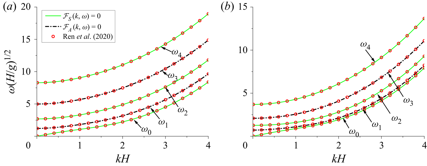
Figure 2. Dispersion relations of the ice-covered channel: (a) clamped–clamped edges; (b) free–free edges. Here,  $b/H=2$ and $h_i/H=1/50$.
Figure 2 verifies the present method and equation numerically. In fact, we can further show that although the present expression for the dispersion relation is different from that in Ren et al. (Reference Ren, Wu and Li2020), they are identical mathematically. To do that, we may first construct a function of the form
 \begin{equation} h(\alpha) = \frac{\alpha^{2}\sinh\alpha H}{K(\alpha,\omega)}\times\frac{\zeta^{2}(\alpha)}{\sigma\tan\sigma b} \end{equation}
in the complex plane  $\alpha$, where $\sigma =-\textrm {i}(k^{2}-\alpha ^{2})^{1/2}$ and
 \begin{equation} \zeta(\alpha)=\left\{
\begin{array}{@{}ll} 1, &
\text{clamped\unicode{x2013}clamped},\\
\sigma^{2}+\nu k^{2}, & \text{free\unicode{x2013}free}.
\end{array} \right. \end{equation}
\begin{equation} \zeta(\alpha)=\left\{
\begin{array}{@{}ll} 1, &
\text{clamped\unicode{x2013}clamped},\\
\sigma^{2}+\nu k^{2}, & \text{free\unicode{x2013}free}.
\end{array} \right. \end{equation}
Consider the integral of  $h(\alpha )$ along a circle $C_R$ of radius $R \to +\infty$ and centred at the origin in the complex plane. Applying the residue theorem at singularities of $K(\alpha,\omega )$ and $\sigma \tanh \sigma b$, we have
 \begin{equation} \frac{1}{2{\rm \pi} {\rm i}}\oint_{C_R}h(\alpha)\, {{\rm d}} \alpha=2\left[ \sum_{m={-}2}^{+\infty}\frac{\kappa_m^{2}\sinh\kappa_mH}{K^{\prime}(\kappa_m, \omega)}\,\frac{\zeta_m^{2}(k)}{\sigma_m\tan\sigma_mb}+\sum_{n=0}^{+\infty} \frac{\alpha_{2n}\sinh\alpha_{2n}H}{K(\alpha_{2n},\omega)}\, \frac{\zeta^{2}(\alpha_{2n})}{b(1+\delta_{n0})}\right], \end{equation}
where  $\alpha _n=(k^{2}+n^{2}{\rm \pi} ^{2}/4b^{2})^{1/2}$. When $R\to +\infty$, $|h(\alpha )|\sim O(1/R^{4})$ for clamped–clamped edges and $|h(\alpha )|\sim O(1/R^{2})$ for free–free edges. Thus the integral in (4.4) tends to zero. Then, using (A4) and (3.23a), we further obtain
 \begin{equation} \mathcal{F}_S(K,\omega)={-}2\sum_{m={-}2}^{+\infty}\frac{\kappa_m^{2} \tanh^{2}\kappa_mH}{Q_m\sigma_m}\,\frac{\zeta_m^{2}(k)}{\tan\sigma_mb}= \frac{4\rho \omega^{2}}{b}\sum_{n=0}^{+\infty}\frac{\alpha_{2n} \sinh\alpha_{2n}H}{K(\alpha_{2n},\omega)}\,\frac{\zeta^{2}(\alpha_{2n})}{(1+\delta_{n0})}. \end{equation}
Similarly,  $\mathcal {F}_A(K,\omega )$ in (3.23b) can be expressed as
 \begin{equation} \mathcal{F}_A(K,\omega)=2\sum_{m={-}2}^{+\infty}\frac{\kappa_m^{2}\tanh^{2} \kappa_mH}{Q_m\sigma_m}\,\frac{\zeta_m^{2}(k)}{\cot\sigma_mb}= \frac{4\rho \omega^{2}}{b}\sum_{n=0}^{+\infty}\frac{\alpha_{2n+1} \sinh\alpha_{2n+1}H}{K(\alpha_{2n+1},\omega)}\,\zeta^{2}(\alpha_{2n+1}). \end{equation}
The system of linear equations in (2.24) in Ren et al. (Reference Ren, Wu and Li2020) can be split into those for symmetric and antisymmetric modes, respectively. Noticing that coefficient  $\varDelta _n$ in (2.20 $a$) in their work can be linked to $K(\alpha,\omega )$ in (3.7) here as $\varDelta _n=-16b^{4}\,K(\alpha _n,\omega )/n^{4}{\rm \pi} ^{4}$ ( $n>0$), through some algebra, it can be shown that $\textrm {det}(\boldsymbol {A})=0$ in (2.25) of Ren et al. (Reference Ren, Wu and Li2020) gives the same series as those on the right-hand sides of (4.5) and (4.6). The above analysis shows that the two different methods give the same dispersion relation, while the present formulations in (4.5) and (4.6) are in a much neater and direct forms. It should also be noted that the other edge conditions can be dealt with in a similar way.
4.2. The natural frequencies at different channel widths and ice sheet thickness
It may also be interesting to investigate how the natural frequencies  $\omega _c^{(i)}$ vary with the channel width $b$ and ice sheet thickness $h_i$. As an example, $\omega _c^{(i)}$ ( $i=1,2,3,4$) under free–free edges are given in figure 3. It can be seen from figure 3(a) that all the $\omega _c^{(i)}$ decrease as $b$ increases. At sufficiently large values of $b/H$, all the $\omega _c^{(i)}$ ( $i=1,2,3,4$) will tend to zero. The natural frequencies at different $h_i$ are given in figure 3(b), and values at $h_i/H=0$ correspond to those of the free surface channel. It can be observed that $\omega _c^{(1)}$ is hardly affected by $h_i$. The effect of ice sheet thickness on $\omega _c^{(i)}$ becomes more apparent when $i$ increases.

Figure 3. Natural frequencies of the ice-covered channel under free–free edges: (a) variation with  $b$ at $h_i/H=1/50$; (b) variation with $h_i$ at $b/H=2$.
4.3. Forces on a cylinder standing at the centre of the channel
Hydroelastic wave diffraction by a vertical circular cylinder standing at the centre of the channel is considered in this subsection. Since the problem is symmetric about  $y=0$, we have $b_{n,m}=b_{-n,m}$ in (3.37). In such a case, the infinite series in (3.41)–(3.43) about $n$ and $n^{\prime }$ need to be considered only from $0$ to $+\infty$. Also, the coefficients $\mathcal {C}_{n,n^{\prime },m}$ and $\mathcal {D}_{n,n^{\prime },m,m^{\prime }}$ given in (3.35) can be further simplified as
 \begin{gather} \mathcal{C}_{n,n^{\prime},m}=\frac{({-}1)^{n}+({-}1)^{n^{\prime}}}{Q_m(1+ \delta_{n0})(1+\delta_{n^{\prime}0})}\int_{0}^{+\infty} \frac{{\rm e}^{-{\rm i}\sigma_mb}\cos n\gamma_m\cos n^{\prime} \gamma_m}{\sigma_m\sin\sigma_mb}\, {{\rm d}}k, \end{gather}
 \begin{gather}\mathcal{D}_{n,n^{\prime},m,m^{\prime}}=\frac{2[({-}1)^{n} +({-}1)^{n^{\prime}}]}{Q_mQ_{m^{\prime}}(1+\delta_{n0})(1+ \delta_{n^{\prime}0})}\int_{\mathscr{L}}\frac{I_mI_{m^{\prime}}\cos n\gamma_m\cos n^{\prime}\gamma_{m^{\prime}}}{\mathcal{F}_S(k, \omega)\sin\sigma_mb\sin\sigma_{m^{\prime}}b}\, {{\rm d}}k. \end{gather}
As expected,  $\mathcal {F}_A(k,\omega )$ does not appear here. Its singularities have no effect or there will be no wave antisymmetric about $y=0$. Furthermore, noticing that $\mathcal {C}_{2n,2n^{\prime }+1,m}=\mathcal {C}_{2n+1,2n^{\prime },m}=\mathcal {D}_{2n,2n^{\prime }+1,m,m^{\prime }}=\mathcal {D}_{2n+1,2n^{\prime },m,m^{\prime }}$ ( $n,n^{\prime }=0,1,2,\ldots$), the unknown coefficients $b_{2n,m}$, $c_{2n}$ and $d_{2n}$ in (3.41)–(3.43) are completely independent of $b_{2n+1,m}$, $c_{2n+1}$ and $d_{2n+1}$.
We first investigate the hydrodynamic forces and vertical shear force at different channel widths when the ice sheet is clamped to the surface of the vertical cylinder. The numerical results for wave forces are shown in figure 4, where the black solid lines correspond to forces on a single vertical circular cylinder standing in the unbounded ocean with an ice cover, which is calculated using the method in Ren et al. (Reference Ren, Wu and Li2020) (as below). Here,  $F_x^{*}$ is defined as $F_x^{*}=F_x/\rho g a^{2}A$; similarly, $M_y^{*}=M_y/\rho ga^{3}A$ and $V^{*}=V/\rho gaA$. When $b/a=5$, it can be seen that $F_x^{*}$ values in two different sets of edge conditions along the tank walls are both significantly different from that in the unbounded ice-covered ocean. In particular, as shown in figure 4(b) for channels with clamped–clamped edges, a couple of peaks can be observed in the curve of $F_x^{*}$ versus $\kappa _0a$. By contrast, there is only one obvious peak in the curve given in figure 4(a) for free–free edges. As $b$ increases, the peaks decrease and gradually become less visible. The curve of $F_x^{*}$ versus $\kappa _0a$ generally shows a variation trend similar to that in the unbounded ocean but with a continuous fluctuation, where the amplitude of fluctuation becomes smaller as $b$ increases. When $b$ is sufficiently large, the results in both cases tend to that in the unbounded ice-covered ocean, which shows that the effects from two side walls and edge conditions at $y=\pm b$ on the hydrodynamic forces become very insignificant. In addition to $F_x^{*}$, similar phenomena can also be observed in the curve of $M_y^{*}$ shown in figure 5.
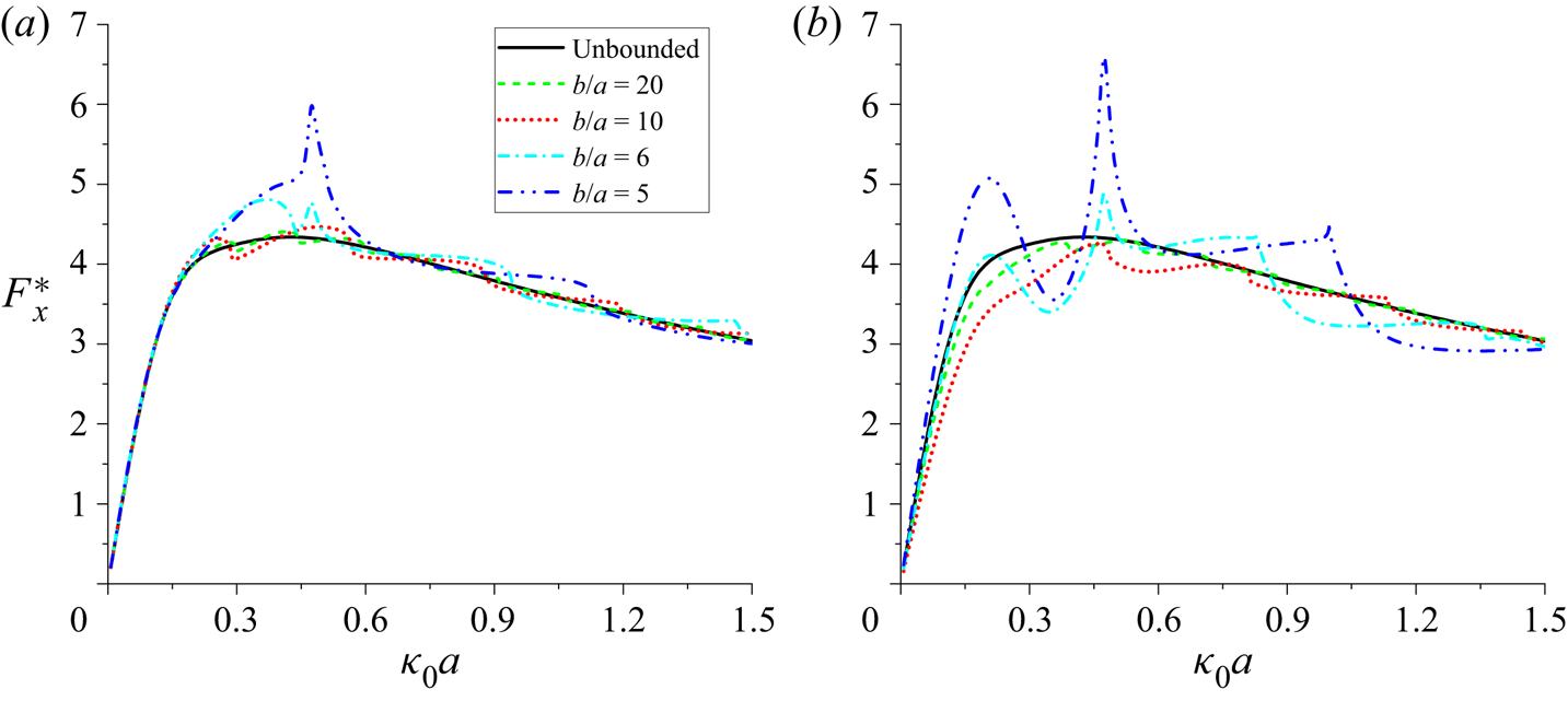
Figure 4. Wave forces in the  $x$-direction on the cylinder at the centre of the channel with different widths, when the ice sheet is clamped to the cylinder: (a) channel with free–free edges; (b) channel with clamped–clamped edges. Here, $H/a=5$ and $h_i/a=1/10$.

Figure 5. Moments in the  $y$-direction on the cylinder at the centre of the channel with different widths, when the ice sheet is clamped to the cylinder: (a) channel with free–free edges; (b) channel with clamped–clamped edges. Here, $H/a=5$ and $h_i/a=1/10$.
The results for the vertical shear forces on the cylinder are shown in figure 6. It may seem to be a surprise that the variation trend of  $V^{*}$ versus $\kappa _0a$ is quite different from that of $F_x^{*}$ and $M_y^{*}$ given in figures 4 and 5. As $\kappa _0a$ increases, $V^{*}$ in the unbounded ice-covered ocean varies smoothly. However, the results in the ice-covered channel oscillate persistently. In particular, rapid changes can be observed when $\kappa _0a$ is close to one of natural frequencies of the channel. This rapid change always exists even when $b$ is sufficiently large, which means that the results for $V^{*}$ will always be different from those in the unbounded ice-covered ocean. The difference between two neighbouring natural frequencies becomes smaller when $b$ is larger. Correspondingly, more oscillatory behaviour of the curves at larger $b$ can be observed in figure 6.

Figure 6. Vertical shear forces on the cylinder at the centre of the channel with different widths, when the ice sheet is clamped to the cylinder: (a) channel with free–free edges; (b) channel with clamped–clamped edges. Here,  $H/a=5$ and $h_i/a=1/10$.
To explain the differences between the behaviours of  $F_x^{*} (M_y^{*})$ and $V^{*}$ when $\kappa _0a$ is near a natural frequency, we may have a closer look at the behaviour of coefficient $\mathcal {D}_{n,n^{\prime },m,m^{\prime }}$ in (4.7b), which is from the Green function in (3.34). It can be seen from (3.46) and (3.49) that $F_x^{*} (M_y^{*})$ is related to $b_{\pm 1,m}$, $c_{\pm 1}$ and $d_{\pm 1}$, while $V^{*}$ is related to $d_0$. As mentioned above, the system of linear equations for $b_{2n,m}$, $c_{2n}$ and $d_{2n}$ is independent of that of $b_{2n+1,m}$, $c_{2n+1}$ and $d_{2n+1}$. Thus $F_x^{*} (M_y^{*})$ is in fact related only to $\mathcal {D}_{2n+1,2n^{\prime }+1,m,m^{\prime }}$ ( $n,n^{\prime }=0,1,2\ldots$), while $V^{*}$ is related only to $\mathcal {D}_{2n,2n^{\prime },m,m^{\prime }}$. From (4.7b), when $\omega =\omega _c^{(2i)}$ ( $i=1,2,3\ldots$), the residue term of $\mathcal {D}_{2n+1,2n^{\prime }+1,m,m^{\prime }}$ corresponding to wave component $k=0$ gives
 \begin{equation} \lim_{k\to 0}\frac{I_m(k)\,I_{m^{\prime}}(k)\cos(2n+1)\gamma_m \cos(2n^{\prime}+1)\gamma_{m^{\prime}}}{\mathcal{F}_S^{\prime}(k, \omega_c^{(2i)})\sin\sigma_mb\sin\sigma_{m^{\prime}}b}=0, \end{equation}
where  $\gamma _m\to {\rm \pi}/2$ when $k\to 0$, which can be seen from (3.32a,b), and $\mathcal {F}_S^{\prime }(k,\omega _c^{(2i)})\sim O(k)$ Thus $\mathcal {D}_{2n+1,2n^{\prime }+1,m,m^{\prime }}$ is bounded at natural frequencies. However, for the residue term of $\mathcal {D}_{2n,2n^{\prime },m,m^{\prime }}$, we obtain
 \begin{equation} \lim_{k\to 0}\frac{I_m(k)\,I_{m^{\prime}}(k)\cos 2n\gamma_m \cos 2n^{\prime}\gamma_{m^{\prime}}}{\mathcal{F}_S^{\prime}(k, \omega_c^{(2i)})\sin\sigma_mb\sin\sigma_{m^{\prime}}b}= \frac{({-}1)^{n+n^{\prime}}I_m(0)\,I_{m^{\prime}}(0)}{\sin\kappa_mb \sin\kappa_{m^{\prime}}b}\,\frac{1}{\mathcal{F}_S^{\prime}(0, \omega_c^{(2i)})}\to\infty. \end{equation}
This indicates that  $\mathcal {D}_{2n,2n^{\prime },m,m^{\prime }}$ are singular at natural frequencies. Since the behaviours of $\mathcal {D}_{2n,2n^{\prime },m,m^{\prime }}$ and $\mathcal {D}_{2n+1,2n^{\prime }+1,m,m^{\prime }}$ at natural frequencies are different, one is regular and the other singular, the behaviours of $F_x^{*}(M_y^{*})$ and $V^{*}$ are also not expected to be the same. On the other hand, as shown in § 3.5, although singular terms existing in the original boundary integral equation, it can be modified into a regular equation and the solution $\phi$ is still finite when $\varGamma \neq 0$. For this case, it is found that $\varGamma$ is indeed non-zero over the full range of $\kappa _0a$ in figure 6. Thus at the natural frequencies, we may use the modified equation given in (3.58) to find the vertical shear force $V^{*}$. The results at several natural frequencies for $b/a=10$ and $20$ are presented in table 1. It is also interesting to see the effect of the edge conditions at the channel walls on $V^{*}$. When the channel is relatively narrow or $b/a =5$ and $10$, significant differences in the curves of $V^{*}$ can be observed in figures 6(a) and 6(b), which indicates that the effect of edge conditions at the channel walls on $V^{*}$ is very strong. As $b$ increases, this effect gradually becomes weaker, and the curves in these two cases show a closer trend.
Table 1. Vertical shear forces at natural frequencies when the ice sheet is clamped to the surface of cylinder but free–free on two side walls. (Here,  $H/a=5$ and $h_i/a=1/10$).

We next consider the cases with different combinations of ice edge conditions on the channel walls and on the cylinder surface. The results for  $F_x^{*}$ and $M_y^{*}$ are given in figure 7 as an example. It can be observed that the curves of wave force and moment vary relatively smoothly when the ice edge is free both on the cylinder surface and on the two channel walls, while there are obvious peaks in the curves of the other three cases. When $\kappa _0a$ is small, the influence of edge conditions on $F_x^{*}$ and $M_y^{*}$ is relatively weak, while it is very strong when $\kappa _0a$ is relatively large.

Figure 7. Wave forces and moments on the cylinder under different types of edge conditions: (a) wave forces; (b) moments. Here, X and Y in X-Y refer the edge conditions on the channel walls and cylinder, respectively, where F means free edge, and C means clamped edge. Here,  $b/a=5$, $H/a=5$ and $h_i/a=1/10$.
We then consider the hydrodynamic forces at different ice sheet thicknesses. A comparison with the hydrodynamic force in the free surface case is given in figure 8, where the corresponding results are calculated through the procedures given in Linton et al. (Reference Linton, Evans and Smith1992). In figure 8(a), the ice edge is free at all boundaries. When  $h_i/a=1/10$, some difference from the result of the free surface case can be observed. As $h_i$ decreases, the difference is very much reduced. When $h_i/a=1/1000$, the difference between the two curves becomes hardly visible. By contrast, the results in figure 8(b) for the ice edges clamped into all boundaries are quite different. Here, $F_x^{*}$ is significantly influenced by $h_i$. There are obvious local peaks in the curve of $h_i/a=1/10$. These peaks decrease or become hardly visible when $h_i/a=1/100$ and $1/1000$. Furthermore, even when the ice sheet becomes very thin at $h_i/a=1/1000$, there are still some visible differences between the results of this case and the free surface case. This indicates that the cases with free edges may resemble the free surface case better when the ice sheet thickness decreases. A similar phenomenon is also reported by Ren et al. (Reference Ren, Wu and Li2020) for the wave diffraction problem of multiple circular cylinders in the unbounded ocean with ice cover.

Figure 8. Wave forces in the  $x$-direction on the cylinder at the centre of the channel with different thicknesses of the ice sheet: (a) edge conditions FF-F; (b) edge conditions CC-C. Here, $b/a=5$ and $H/a=5$.
4.4. Forces on a cylinder standing in off-centre positions of the channel
Computations are also carried out to investigate the forces on a vertical cylinder standing in off-centre positions of the channel. In such a case, both the poles caused by the symmetric modes or  $\mathcal {F}_S (k,\omega )=0$, and the antisymmetric modes or $\mathcal {F}_A (k,\omega )=0$, will exist in the coefficients $\mathcal {D}_{n,n^{\prime },m,m^{\prime }}$ given in (3.35b). Here, we may give an example of the case when the ice sheet is free along two side walls and is clamped into the surface of the cylinder. The numerical results for hydrodynamic forces are presented in figure 9. In figure 9(a), the curves of $F_x^{*}$ versus $\kappa _0a$ show small differences only at $y_c/a=0$, $2$ and $4$. However, if the cylinder moves to the channel wall further, or at $y_c=6$ and $8$,
$8$,  $F_x^{*}$ at some $\kappa _0a$ is significantly increased. Similar to the case at $y_c=0$, $F_x^{*}$ still varies relatively smoothly when $y_c\neq 0$. By contrast, obvious local peaks and rapid changes can be observed in the curves of $F_y^{*}$ shown in figure 9(b) when $\kappa _0a$ approaches the values corresponding to the natural frequencies of the channel. A similar phenomenon also occurs in the vertical shear force provided in figure 10. Compared with the results at $y_c=0$, since both $\omega _c^{(2i)}$ and $\omega _c^{(2i-1)}$ ( $i=1,2,3,\ldots$) will affect $V^{*}$, more peaks in $V^{*}$ can be seen. In fact, if we define $b_{n,m}^{\pm }=b_{n,m}\pm (-1)^{n}b_{-n,m}$, $c_n^{\pm }=c_n\mp (-1)^{n}c_{-n}$ and $d_n^{\pm }=d_n\mp (-1)^{n}d_{-n}$ ( $n=0,1,2,\ldots$), the matrix equation in (3.41)–(3.43) for $b_{n,m}$, $c_n$ and $d_n$ can be further converted into two independent submatrix equations. The one for $b_{n,m}^{+}$, $c_n^{+}$ and $d_n^{+}$ has singular terms at natural frequencies, and it is related to $F_y^{*}$ and $V^{*}$. The other, for $b_{n,m}^{-}$, $c_n^{-}$ and $d_n^{-}$, is regular and related to $F_x^{*}$. Thus different behaviours are observed from $F_x^{*}$ and $F_y^{*}$ & $V^{*}$ in figures 9 and 10 when $\omega$ is near a natural frequency.
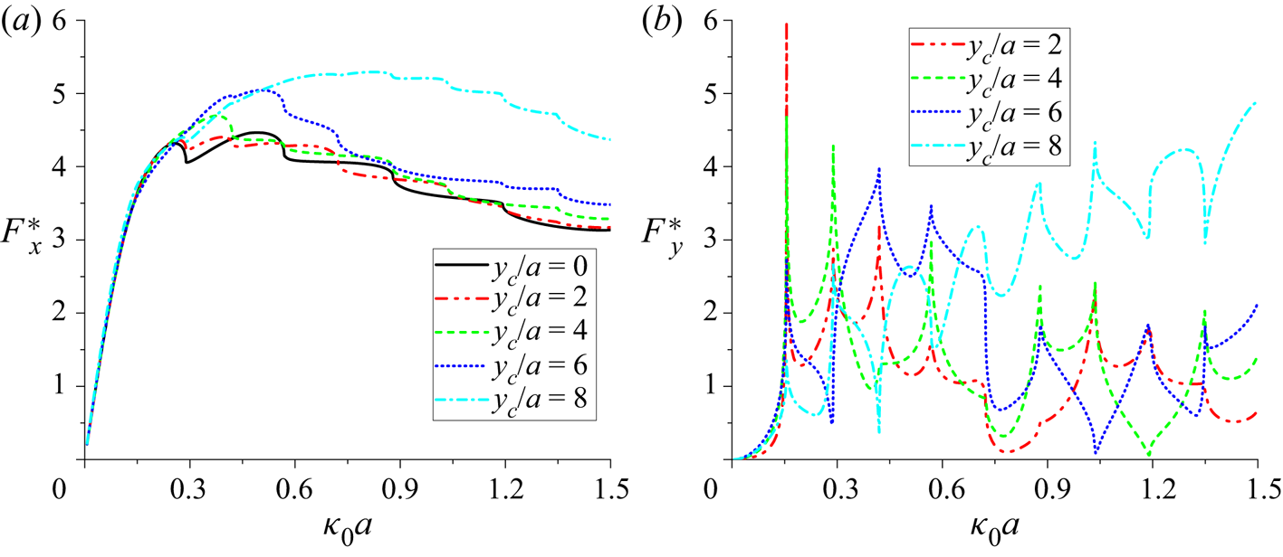
Figure 9. Wave forces on the cylinder at various off-centre positions of the channel, for edge conditions FF-C: (a) force in the  $x$-direction; (b) force in the $y$-direction. Here, $b/a=10$, $H/a=5$ and $h_i/a=1/10$.

Figure 10. Vertical shear forces on the cylinder at various off-centre positions of the channel, for edge conditions FF-C. Here,  $b/a=10$, $H/a=5$ and $h_i/a=1/10$.
4.5. Wave patterns and principal strain distributions in the ice-covered channel
The wave elevation or ice sheet deflection can be obtained from  $\eta =-({i}/{\omega })({\partial \phi }/{\partial z})|_{z=0}$, together with (3.44). We have
 \begin{align} \eta(r,\theta)\!&=\!{-}\frac{\rm \pi}{2\omega}\sum_{n={-}\infty}^{+\infty} \sum_{m={-}2}^{+\infty}\frac{b_{n,m}\kappa_m\tanh\kappa_mH}{Q_m} \left[\frac{\mathscr{H}_n^{(1)}(\kappa_mr)}{\mathcal{J}_n(\kappa_mr)}- \frac{\mathscr{H}_n^{(1)\prime}(\kappa_ma)}{\mathcal{J}_n^{\prime} (\kappa_ma)}\right]\mathcal{J}_n(\kappa_mr)\, {\rm e}^{-{\rm i}n\theta}\nonumber\\ &\quad +\frac{{\rm i}L}{\rho \omega^{3}}\sum_{n={-}\infty}^{+\infty} \sum_{m={-}2}^{+\infty}\frac{(\kappa_m^{2}c_n+d_n)\kappa_m\tanh^{2}\kappa_mH}{Q_m}\, \frac{\mathcal{J}_n(\kappa_mr)}{\mathcal{J}_n^{\prime}(\kappa_ma)}\, {\rm e}^{{\rm i}n\theta}. \end{align}
An example of  $|\eta |/A$ at $\kappa _0a=0.8$ under four different combinations of edge conditions is provided in figure 11, where the vertical cylinder is located at the centre of the channel. It can be seen that the wave pattern is affected significantly by the edge conditions. In figure 11(a), when the ice edges are free at all boundaries, the maximum amplitude may occur at the front surface of the vertical cylinder or at two side walls. In figure 11(b), if the ice sheet is clamped to the cylinder, then the wave amplitude on its surface will be zero, and then the maximum amplitude may occur at the region in front of the cylinder or at two side walls. By contrast, when the ice edges are clamped to two channel walls, as given in figures 11(c) and 11(d), the maximum wave amplitude may appear only on the front surface or front region of the cylinder.

Figure 11. Wave amplitude  $|\eta |/A$ in the ice-covered channel at $\kappa _0a=0.8$ under different edge conditions: (a) FF-F; (b) FF-C; (c) CC-F; (d) CC-C. Here, $b/a=10$, $H/a=5$ and $h_i/a=1/10$.
The strain of the ice sheet is also a very important physical parameter related to the fracture and breakup of the ice. The principal strain  $\boldsymbol {\epsilon }$ can be calculated by determining the eigenvalues of the strain tensor matrix (Fung Reference Fung1977)
 \begin{equation} \boldsymbol{\epsilon} = \frac{h_i}{2}\left[ \begin{array}{cc} \epsilon_{rr} & \epsilon_{r\theta}\\ \epsilon_{r\theta} & \epsilon_{\theta\theta}\\ \end{array} \right]=\frac{h_i}{2}\left[ \begin{array}{cc} \dfrac{\partial^{2} W}{\partial r^{2}} & \dfrac{\partial^{2} W}{r\,\partial r\,\partial \theta}-\dfrac{\partial W}{r^{2}\,\partial \theta}\\[6pt] \dfrac{\partial^{2} W}{r\,\partial r\,\partial \theta}-\dfrac{\partial W}{r^{2}\,\partial \theta} & \dfrac{\partial W}{r\,\partial r}+\dfrac{\partial^{2}W}{r^{2}\,\partial\theta^{2}}\\ \end{array} \right], \end{equation}
where the ice sheet deflection  $W(r,\theta,t)$ can be expressed as
 \begin{equation} W(r,\theta,t)={\rm Re}\{\eta(r,\theta)\, {\rm e}^{{\rm i}\omega t}\} ={\rm Re}\{\eta(r,\theta)\}\cos\omega t - {\rm Im} \{\eta(r,\theta)\}\sin\omega t. \end{equation}
The eigenvalues  $\varsigma _{1,2}$ of the strain tensor matrix $\boldsymbol {\epsilon }$ can be obtained as
 \begin{align} \varsigma_{1,2}&=\frac{h_i}{4}\left\{\left(\frac{\partial^{2} W}{\partial r^{2}}+ \frac{\partial W}{r\,\partial r}+\frac{\partial^{2}W}{r^{2}\,\partial\theta^{2}}\right) \pm\left[\left(\frac{\partial^{2} W}{\partial r^{2}}-\frac{\partial W}{r\,\partial r}- \frac{\partial^{2}W}{r^{2}\,\partial\theta^{2}}\right)^{2}\right.\right.\nonumber\\ &\quad \left.\left.{}+4 \left(\frac{\partial^{2} W}{r\,\partial r\,\partial \theta}- \frac{\partial W}{r^{2}\,\partial \theta}\right)^{2}\right]^{1/2}\right\}. \end{align}
 Substituting (4.12) and (4.10) into (4.13), the maximum principal strain  $\epsilon _{max}$ at a given location can be found as the maximum value of $|\varsigma _{1,2}|$ as $t$ varies from $0$ to $2{\rm \pi} /\omega$. The distributions of $\epsilon _{max}$ at $\kappa _0a=0.8$ under four different combinations of edge conditions are given in figure 12. Compared with figure 11, the position of the largest value of $\epsilon _{max}$ is different from that of $|\eta |/A$. In figures 12(b) and 12(d), when the ice sheet is clamped to the surface of the cylinder, the largest $\epsilon _{max}$ is at the front surface of the vertical cylinder. However, when the ice sheet is free on the cylinder surface, the largest $\epsilon _{max}$ is on the left and right sides of the cylinder, as shown in figures 12(a) and 12(c).

Figure 12. Distribution of the maximum principal strain  $\epsilon _{max}$ in the ice-covered channel at $\kappa _0a=0.8$ under different edge conditions: (a) FF-F; (b) FF-C; (c) CC-F; (d) CC-C. Here, $b/a=10$, $H/a=5$ and $h_i/a=1/10$.
5. Conclusions
The problem of hydroelastic wave diffraction by a vertical circular cylinder standing in an ice-covered channel has been studied analytically. The solution procedure is applicable to various ice edge conditions and their combinations. The Green function satisfying all the boundary conditions apart from that on the body surface is first derived based on the method of eigenfunction expansion in the vertical direction. With the help of the Green function, a general source distribution formula for surface-piercing structures with arbitrary shapes in fluid with an ice cover is established, which involves integrals over the body surface and its intersection with the ice sheet. If the structure is a vertical cylinder mounted to the bottom of the channel and has a constant cross-section along the depth direction, then the source distribution formula can be simplified further by using an inner product. Based on this formula, the velocity potential due to a vertical circular cylinder is expressed explicitly as an infinite series with unknown coefficients, which can be solved from the impermeable condition on the body surface and the conditions at the ice edge contacting the body surface.
From the solution of the Green function, it is confirmed that the dispersion relation obtained is identical mathematically to that in Ren et al. (Reference Ren, Wu and Li2020), but the formulation in the present work is much neater. The natural frequency of the ice-covered channel is defined in a similar way to that of free surface channels. There are an infinite number of natural frequencies, and at any one of them, the Green function will be singular, which further leads to a singular term in the boundary integral equation of the velocity potential due to a vertical circular cylinder. To treat this, a revised non-singular matrix equation with a parameter  $\varGamma$ is established. The velocity potential will still be bounded at the natural frequencies when $\varGamma \neq 0$.
From the results of the hydroelastic wave diffraction by a vertical circular cylinder, it is found that both the hydrodynamic forces  $F_x^{*}$, $F_y^{*}$ and the vertical shear force $V^{*}$ on the cylinder are all significantly affected by the channel width $b$ and ice sheet thickness $h_i$, as well as the edge conditions on the body surface and channel walls. The numerical results are also compared with those in the unbounded ocean with an ice cover and in the free surface channel. It is observed that $F_x^{*}$ will tend to the result in the bounded ice-covered ocean when $b\to +\infty$, and tend to the result in the free surface channel when $h_i\to 0$. The behaviour of $F_x^{*}$ is different from that of $F_y^{*}$ and $V^{*}$ near the natural frequency; $F_x^{*}$ varies relatively smoothly when $\kappa _0a$ is near the natural frequency, because the singularity of the Green function at the natural frequency does not affect the coefficient in the equation of $F_x^{*}$. Obvious peaks and sudden changes near the natural frequencies can be observed in the curves of $F_y^{*}$ versus $\kappa _0a$, and $V^{*}$ versus $\kappa _0a$, as the singularity of the Green function does affect the coefficients in the equation of $F_y^{*}$ and $V^{*}$. However, $F_y^{*}$ and $V^{*}$ are not singular at the natural frequency when $\varGamma \neq 0$. The sudden change of $V^{*}$ always exists even when $b$ is very large, which makes the curves of $V^{*}$ versus $\kappa _0a$ always different from those in the unbounded ocean.
The present work has focused a single vertical circular cylinder. The formulation can be extended easily to multiple vertical circular cylinders if Graf's addition theorem for the Bessel functions is used, as in Ren et al. (Reference Ren, Wu and Ji2018a). For a vertical cylinder of arbitrary cross-section, the vertical modes for the source distribution can be still used, while numerical discretization can be used in the circumferential direction. For a body of a general shape, the boundary element method can be used based on the Green function derived in the work.
Acknowledgements
Y.F.Y. is grateful to Lloyd's Register Foundation and China Scholarships Council for sponsoring his PhD study.
Declaration of interests
The authors report no conflict of interest.
Funding
The work is supported by Lloyd's Register Foundation. The LRF helps to protect life and property by supporting engineering-related education, public engagement and the application of research.
Appendix A. The series form of the Green function in unbounded problems
To convert the integral in (3.5) into a summation, we may consider the integration
 \begin{equation} I_R = \oint_{\varGamma_R}\frac{{\rm e}^{-{\rm i}\sigma|y-y_0|}\,f (\alpha,z_>,z_<)}{\alpha\,K(\alpha,\omega)}\, {{\rm d}} \sigma, \end{equation}
where the integration loop  $\varGamma _R$ is first along the real axis from $(-R,0)$ to $(R,0)$, and then clockwise along a semicircle of radius $R$ centred at the origin. The integration path at the real axis should pass under (over) the poles at $\sigma =-(\kappa _0^{2}-k^{2})^{1/2}$ ( $\sigma =+(\kappa _0^{2}-k^{2})^{1/2}$) when $\kappa _0>k$. When $R\to +\infty$, the integrand decays exponentially, thus only the integral along the real axis remains in $I_R$, or
 \begin{equation} \lim_{R\to+\infty}I_R = \int_{-\infty}^{+\infty}\frac{{\rm e}^{-{\rm i} \sigma|y-y_0|}\,f(\alpha,z_>,z_<)}{\alpha\,K(\alpha,\omega)}\, {{\rm d}} \sigma. \end{equation}
Applying the residue theorem to (A1) and noticing the additional poles in the complex plane where  $K(\alpha,\omega )=0$, we have
 \begin{equation} \lim_{R\to+\infty}\oint_{\varGamma_R}\frac{{\rm e}^{-{\rm i} \sigma|y-y_0|}\,f(\alpha,z_>,z_<)}{\alpha\,K(\alpha,\omega)}\, {{\rm d}} \sigma={-}2{\rm \pi}{\rm i}\sum_{m={-}2}^{+\infty}\frac{{\rm e}^{-{\rm i} \sigma_m|y-y_0|}\,f(-\kappa_m,z_>,z_<)}{\sigma_m\,K^{\prime}(-\kappa_m,\omega)}, \end{equation}
where the prime denotes the derivative with respect to  $\alpha$. Using
 \begin{gather} K^{\prime}(\kappa_m,\omega)=\frac{2\rho\omega^{2}\cosh^{2} \kappa_mH}{\sinh\kappa_mH}\,Q_m, \end{gather}
 \begin{gather}f(\kappa_m,z_>,z_<)=\frac{\rho\omega^{2}\cosh\kappa_m(z+H)\cosh \kappa_m(z_0+H)}{\sinh\kappa_mH}, \end{gather}
we have
 \begin{equation} \int_{-\infty}^{+\infty}\frac{{\rm e}^{-{\rm i}\sigma|y-y_0|}\, f(\alpha,z_>,z_<)}{\alpha\,K(\alpha,\omega)}\, {{\rm d}} \sigma ={-}2{\rm \pi}{\rm i}\sum_{m={-}2}^{+\infty}\frac{{\rm e}^{-{\rm i} \sigma_m|y-y_0|}\,\psi_m(z)\,\psi_m(z_0)}{2\sigma_mQ_m}, \end{equation}
where  $\psi _m(z)$ and $Q_m$ are defined in (3.9) and (3.10), respectively. This shows that (3.5) is identical to (3.8).
Appendix B. Elements of the matrix equation in (3.20)
The elements of matrix  $A_{ij}$ and column $B_j$ ( $i,j=1,2,3,4$) in (3.20) under different edges are given below. For clamped–clamped edges, we have
 \begin{gather} A_{1j}=\frac{L}{\rho\omega^{2}}\sum_{m={-}2}^{+\infty} \frac{\kappa_m^{2}\tanh^{2}\kappa_mH}{Q_m\sigma_m}\times \left[-\frac{(\kappa_m^{2}\delta_{j1}+\delta_{j2})}{\tan\sigma_mb} +\frac{(\kappa_m^{2}\delta_{j3}+\delta_{j4})}{\cot\sigma_mb}\right], \end{gather}
 \begin{gather}A_{2j}=\frac{L}{\rho\omega^{2}}\sum_{m={-}2}^{+\infty} \frac{\kappa_m^{2}\tanh^{2}\kappa_mH}{Q_m\sigma_m}\times \left[-\frac{(\kappa_m^{2}\delta_{j1}+\delta_{j2})}{\tan\sigma_mb}- \frac{(\kappa_m^{2}\delta_{j3}+\delta_{j4})}{\cot\sigma_mb}\right], \end{gather}
 \begin{gather}A_{3j}=\frac{L}{\rho\omega^{2}}\sum_{m={-}2}^{+\infty} \frac{\kappa_m^{2}\tanh^{2}\kappa_mH}{Q_m}\times [\kappa_m^{2}(\delta_{j1}+\delta_{j3})+(\delta_{j2}+\delta_{j4})], \end{gather}
 \begin{gather}A_{4j}=\frac{L}{\rho\omega^{2}}\sum_{m={-}2}^{+\infty} \frac{\kappa_m^{2}\tanh^{2}\kappa_mH}{Q_m}\times [\kappa_m^{2}(\delta_{j3}-\delta_{j1})+(\delta_{j4}-\delta_{j2})], \end{gather}
 \begin{gather} B_j={-}\sum_{m={-}2}^{+\infty}\frac{\psi_m(z_0)\,\kappa_m\tanh\kappa_mH}{Q_m \sigma_m\sin 2\sigma_mb}\times[\delta_{j1}\cos\sigma_m(y_0+b)+ \delta_{j2}\cos\sigma_m(y_0-b)]. \end{gather}
For free–free edges, we obtain
 \begin{gather} A_{1j}=\frac{L}{\rho\omega^{2}}\sum_{m={-}2}^{+\infty} \frac{\kappa_m^{2}\tanh^{2}\kappa_mH}{Q_m}\times\left(\sigma_m+ \frac{\nu k^{2}}{\sigma_m}\right)\left[\frac{(\kappa_m^{2}\delta_{j1}+ \delta_{j2})}{\tan\sigma_mb}-\frac{(\kappa_m^{2}\delta_{j3}+ \delta_{j4})}{\cot\sigma_mb}\right], \end{gather}
 \begin{gather}A_{2j}=\frac{L}{\rho\omega^{2}}\sum_{m={-}2}^{+\infty} \frac{\kappa_m^{2}\tanh^{2}\kappa_mH}{Q_m}\times\left(\sigma_m+ \frac{\nu k^{2}}{\sigma_m}\right)\left[\frac{(\kappa_m^{2}\delta_{j1}+ \delta_{j2})}{\tan\sigma_mb}+\frac{(\kappa_m^{2}\delta_{j3}+ \delta_{j4})}{\cot\sigma_mb}\right], \end{gather}
 \begin{gather}A_{3j}={-}\frac{L}{\rho\omega^{2}}\sum_{m={-}2}^{+\infty} \frac{\kappa_m^{2}\tanh^{2}\kappa_mH}{Q_m}\times[\sigma_m^{2}+(2-\nu)k^{2}] [\kappa_m^{2}(\delta_{j1}+\delta_{j3})+(\delta_{j2}+\delta_{j4})], \end{gather}
 \begin{gather}A_{4j}={-}\frac{L}{\rho\omega^{2}}\sum_{m={-}2}^{+\infty} \frac{\kappa_m^{2}\tanh^{2}\kappa_mH}{Q_m}\times[\sigma_m^{2}+(2-\nu)k^{2}] [\kappa_m^{2}(\delta_{j3}-\delta_{j1})+(\delta_{j4}-\delta_{j2})], \end{gather}
 \begin{gather} B_j=\sum_{m={-}2}^{+\infty}\frac{\psi_m(z_0)\,\kappa_m\tanh\kappa_mH}{Q_m \sin 2\sigma_mb}\!\times\!\left(\sigma_m+\frac{\nu k^{2}}{\sigma_m}\right)[\delta_{j1}\cos\sigma_m(y_0+b)\!+\!\delta_{j2} \cos\sigma_m(y_0-b)]. \end{gather}
Using (Evans & Porter Reference Evans and Porter2003) gives
 \begin{equation} \frac{L}{\rho \omega^{2}}\sum_{m={-}2}^{+\infty}\frac{\kappa_m^{n} \tanh^{2}\kappa_mH}{Q_m}=\left\{ \begin{array}{@{}ll} 0, & n=2,\\ 1, & n=4,\\ 0, & n=6,\\ \end{array} \right. \end{equation}
and  $A_{3j}$ and $A_{4j}$ ( $j=1,2,3,4$) can be simplified further. For clamped–clamped edges, this gives
 \begin{equation} A_{3j}=\delta_{j1}+\delta_{j3}\quad\text{and}\quad A_{4j}={-}\delta_{j1}+\delta_{j3}, \end{equation}
while for free–free edges, we have
 \begin{equation} A_{3j}=(\nu -1)k^{2}(\delta_{j1}+\delta_{j3})-(\delta_{j2}+\delta_{j4}) \quad\text{and}\quad A_{4j}=(\nu -1)k^{2}(\delta_{j3}-\delta_{j1}) -(\delta_{j4}-\delta_{j2}). \end{equation}
From (B1)–(B4), (B6a,b) and (B7a,b),  $\beta _j$ can be solved as
 \begin{equation} \left. \begin{array}{ll@{}} \displaystyle \beta_j = \dfrac{-\delta_{j2}}{2A_{12}}\sum_{m={-}2}^{+\infty} \dfrac{\psi_m(z_0)\,\kappa_m\tanh\kappa_mH}{Q_m\sigma_m}\, \dfrac{\cos\sigma_my_0}{\sin\sigma_mb}, & j=1,2,\\ \displaystyle \beta_j =\dfrac{\delta_{j4}}{2A_{14}}\sum_{m={-}2}^{+\infty} \dfrac{\psi_m(z_0)\,\kappa_m\tanh\kappa_mH}{Q_m\sigma_m}\, \dfrac{\sin\sigma_my_0}{\cos\sigma_mb}, & j=3,4,\\ \end{array} \right\} \end{equation}
for clamped–clamped edges, while
 \begin{equation} \left. \begin{array}{c} \displaystyle\beta_j = \dfrac{\delta_{j1}+\delta_{j2}(\nu-1)k^{2}}{2[A_{11}+(\nu -1)k^{2}A_{12}]}\sum_{m={-}2}^{+\infty}\dfrac{\psi_m(z_0)\,(\sigma_m^{2}+\nu k^{2})\kappa_m\tanh\kappa_mH}{Q_m\sigma_m}\,\dfrac{\cos\sigma_my_0}{\sin\sigma_mb},\quad j=1,2,\\ \displaystyle\beta_j =\dfrac{-\delta_{j3}-\delta_{j4}(\nu -1)k^{2}}{2[A_{13}+(\nu-1)k^{2}A_{14}]}\sum_{m={-}2}^{+\infty}\dfrac{\psi_m(z_0)\,(\sigma_m^{2}+\nu k^{2})\kappa_m\tanh\kappa_mH}{Q_m\sigma_m}\,\dfrac{\sin\sigma_my_0}{\cos\sigma_mb},\quad j=3,4,\\ \end{array} \right\} \end{equation}
for free–free edges.
Appendix C. The source distribution formula for the velocity potential
Applying Green's second identity to the diffracted velocity potential component  $\phi _D$ and the Green function $G$ throughout the fluid domain, we have
 \begin{equation} 2{\rm \pi}\,\phi_D(x_0,y_0,z_0)= \unicode{x222F}_S \left(\phi_D\,\frac{\partial G}{\partial n}-G\,\frac{\partial \phi_D}{\partial n}\right) {{\rm d}}S, \end{equation}
where  $S$ is comprised of the bottom of the channel $S_H$, two vertical side walls $S_W$, the ice sheet $S_I$, two vertical far field boundaries $S_{\pm \infty }$, and the surface of the body $S_B$. By using a similar procedure given in Yang et al. (Reference Yang, Wu and Ren2021), only the integrals over $S_B$ and along the intersection line $\mathcal {L}$ of the ice sheet with the body surface need to be kept on the right-hand side, or
 \begin{align}
& 2{\rm \pi}\,\phi_D(x_0,y_0,z_0)=\frac{L}{\rho
\omega^{2}}\nonumber\\ &\quad
\times\oint_{\mathcal{L}}\left[\frac{\partial G}{\partial
z}\, \frac{\partial }{\partial
n}\left(\nabla^{2}\frac{\partial \phi_D}{\partial
z}\right)- \frac{\partial^{2} G}{\partial z\,\partial
n}\left(\nabla^{2} \frac{\partial \phi_D}{\partial
z}\right)-\frac{\partial \phi_D}{\partial z}\,
\frac{\partial }{\partial n}\left(\nabla^{2}\frac{\partial
G}{\partial z} \right)\right.\nonumber\\ &\quad \left.
+\,\frac{\partial^{2} \phi_D}{\partial z\,\partial
n}\left(\nabla^{2} \frac{\partial G}{\partial
z}\right)\right] {{\rm d}}l\nonumber\\ &\quad
+\iint_{S_B}\left(\phi_D\,\frac{\partial G}{\partial n}-G\,
\frac{\partial \phi_D}{\partial n}\right) {{\rm d}}S.
\end{align}
\begin{align}
& 2{\rm \pi}\,\phi_D(x_0,y_0,z_0)=\frac{L}{\rho
\omega^{2}}\nonumber\\ &\quad
\times\oint_{\mathcal{L}}\left[\frac{\partial G}{\partial
z}\, \frac{\partial }{\partial
n}\left(\nabla^{2}\frac{\partial \phi_D}{\partial
z}\right)- \frac{\partial^{2} G}{\partial z\,\partial
n}\left(\nabla^{2} \frac{\partial \phi_D}{\partial
z}\right)-\frac{\partial \phi_D}{\partial z}\,
\frac{\partial }{\partial n}\left(\nabla^{2}\frac{\partial
G}{\partial z} \right)\right.\nonumber\\ &\quad \left.
+\,\frac{\partial^{2} \phi_D}{\partial z\,\partial
n}\left(\nabla^{2} \frac{\partial G}{\partial
z}\right)\right] {{\rm d}}l\nonumber\\ &\quad
+\iint_{S_B}\left(\phi_D\,\frac{\partial G}{\partial n}-G\,
\frac{\partial \phi_D}{\partial n}\right) {{\rm d}}S.
\end{align}
Using the relationship  $\nabla ^{2}=-\partial ^{2}/\partial z^{2}$ obtained from the Laplace equation, (C2) can be written as
 \begin{align} 2{\rm \pi}\,\phi_D(x_0,y_0,z_0)&\!=\!{-}\frac{L}{\rho \omega^{2}}\oint_{\mathcal{L}} \left[\frac{\partial G}{\partial z}\,\frac{\partial^{4}\phi_D}{\partial n\,\partial z^{3}}\!-\frac{\partial^{2} G}{\partial n\,\partial z}\,\frac{\partial^{3}\phi_D}{\partial z^{3}}\!-\!\frac{\partial \phi_D}{\partial z}\,\frac{\partial^{4} G}{\partial n\,\partial z^{3}}\!+\!\frac{\partial^{2} \phi_D}{\partial n\,\partial z}\, \frac{\partial^{3}G}{\partial z^{3}}\right] {{\rm d}}l\nonumber\\ &\quad +\iint_{S_B}\left(\phi_D\,\frac{\partial G}{\partial n}-G\, \frac{\partial \phi_D}{\partial n}\right) {{\rm d}}S. \end{align}
We may introduce a velocity potential  $\varphi (x,y,z)$ defined inside the vertical cylinder. On $z=0$, $\varphi$ satisfies the ice sheet boundary condition in (2.4). We also have
 \begin{equation} \varphi = \phi_D\quad \text{on } S_B. \end{equation}
At the intersection line  $\mathcal {L}$, the edge conditions can be expressed as
 \begin{equation} \frac{\partial \varphi}{\partial z}=\frac{\partial \phi_D}{\partial z}\quad\text{and}\quad\frac{\partial^{3} \varphi}{\partial z^{3}} = \frac{\partial^{3} \phi_D}{\partial z^{3}},\quad \text{at } \mathcal{L}. \end{equation}
Applying Green's second identity to  $\varphi$ and $G$ in the inner domain, if the source point $(x_0,y_0,z_0)$ is in the outer domain, then we obtain
 \begin{align} 0&={-}\frac{L}{\rho \omega^{2}}\oint_{\mathcal{L}}\left[\frac{\partial G}{\partial z}\,\frac{\partial^{4}\varphi}{\partial n\,\partial z^{3}}-\frac{\partial^{2} G}{\partial n\,\partial z}\,\frac{\partial^{3}\varphi}{\partial z^{3}}-\frac{\partial \varphi}{\partial z}\,\frac{\partial^{4} G}{\partial n\,\partial z^{3}}+\frac{\partial^{2} \varphi}{\partial n\,\partial z}\,\frac{\partial^{3}G}{\partial z^{3}}\right] {{\rm d}}l\nonumber\\ &\quad +\iint_{S_B}\left(\varphi\,\frac{\partial G}{\partial n}-G\,\frac{\partial \varphi}{\partial n}\right) {{\rm d}}S. \end{align}
Subtracting (C6) from (C3) and using conditions in (C4) and (C5), we obtain
 \begin{equation} \phi_D(x_0,y_0,z_0)=\frac{L}{\rho \omega^{2}}\oint_{\mathcal{L}} \left(\frac{\partial G}{\partial z}\,\frac{\partial^{3}\varPsi}{\partial z^{3}}\, +\frac{\partial^{3} G}{\partial z^{3}}\frac{\partial \varPsi}{\partial z}\right) {{\rm d}}l+\iint_{S_B}G\varPsi \, {{\rm d}}S, \end{equation}
where source strength  $\varPsi (x,y,z)$ on the body surface is defined as
 \begin{equation} \varPsi(x,y,z)=\frac{1}{2{\rm \pi}}\left[\frac{\partial \varphi(x,y,z)}{\partial n}-\frac{\partial \phi_D(x,y,z)}{\partial n}\right]. \end{equation}
If the body is a vertical cylinder mounted to the bottom and with a homogeneous section along the  $z$-direction, then we may apply the orthogonal inner product in (3.13) to (C7) and we obtain
 \begin{equation} \phi_D(x_0,y_0,z_0)=\oint_{\mathcal{L}}\langle G(x,y,z;x_0,y_0,z_0), \varPsi(x,y,z)\rangle \, {{\rm d}}l. \end{equation}


 Open access