


1. Introduction
1.1. Competitive rowing
Competitive rowing is an Olympic sport where the differences between the winner and the runners up are very small, usually less than 1 s over a 2000 m race while a race typically lasts 6 min. Since finishing times are so close, small improvements of the hydrodynamic propulsion can have a large impact on the outcome of a race. The optimisation of the propulsion requires a good understanding of the oar blade motion and the flow field around the oar blade, with its corresponding hydrodynamic forces. In this study, we capture the oar blade kinematics during actual on-water rowing and then reproduce the (scaled) motion in a laboratory, which enables the use of advanced flow field measurement techniques, such as particle image velocimetry (PIV), together with simultaneous force measurements.
After the athlete inserts the oar blade in the water and exerts a force on the handle, the oar is pivoting on the oar lock and moves through the water, generating propulsion; this is called the drive phase. Throughout the drive phase the oar blade remains in a vertical position and at a constant depth with its top edge at the height of the otherwise unperturbed free surface. In this study it is assumed that the rowing motion and generated forces are in the horizontal plane ( $x$,
$x$, $y$-plane), because (i) the kinematics during the drive phase are exclusively in this plane, and (ii) it is known that, during on-water rowing, athletes do not need to exert any (significant) vertical force on the oar handle to keep the oar blade at constant depth below the surface. This implies that the resultant force on the rowing oar blade is also solely in the $x$,
$x$, $y$-plane.
The oar blade path follows from the superposition of the pivoting motion of the oar on the motion of the pivot point, i.e. the boat motion, as illustrated in figure 1. In that figure, both the boat velocity and the angular velocity of the oar are taken constant, while in reality both vary in time. The positive  $x$-direction is defined as the direction of the boat motion, the $y$-direction is perpendicular and outwards to that (away from the hull) in the horizontal plane, and the angle $\theta$ defines the oar orientation, where $\theta = 0^{\circ }$ is parallel to the $y$-direction. The oar angle $\theta$ is defined positive in counter-clockwise direction, and thus increases from the catch, e.g. $\theta = -50^{\circ }$, to the release, e.g. $\theta = 30^{\circ }$.
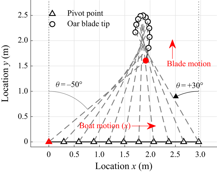
Figure 1. A generic oar blade path composed of the boat motion along a straight line (in the positive  $x$-direction) and the rotation of the oar around a pivot point fixed to the boat (with $\theta = 0^{\circ }$ corresponding to a position of the oar perpendicular to the boat motion). For simplicity, both the angular velocity and the boat velocity are taken as constant for this generic path with $V_{boat} = 3.7\ \textrm {m}\ \textrm {s}^{-1}$ and $\dot {\theta } = 100^{\circ }\ \textrm {s}^{-1}$. The grey dashed lines represent the oar orientation, and the open spheres mark the oar blade tip. The oar blade tip moves in the positive $y$-direction at the catch (red marker) and in the negative $y$-direction during the last part of the stroke.
1.2. Previous research on rowing
The hydrodynamics of a steady flow over an oar blade has been investigated both numerically and experimentally by Caplan & Gardner (Reference Caplan and Gardner2007) and Coppel et al. (Reference Coppel, Gardner, Caplan and Hargreaves2010), but neither account for the presence of a free surface, nor do they account for the accelerations and decelerations of the oar blade, or the strong curvature of the blade path. In the works of Sliasas & Tullis (Reference Sliasas and Tullis2009), Leroyer et al. (Reference Leroyer, Barré, Kobus and Visonneau2010) and Robert et al. (Reference Robert, Leroyer, Barré, Rongère, Queutey and Visonneau2014), the unsteady motion of the oar blade was incorporated in their numerical simulations using commercial software. They all found that the results for unsteady flow differed substantially from steady flow over an oar blade. In the work by Robert et al. (Reference Robert, Leroyer, Barré, Rongère, Queutey and Visonneau2014) the results are benchmarked against unsteady experimental work by Barré & Kobus (Reference Barré and Kobus2010) and were found to match reasonably well only when the free surface and unsteady motion of the oar blade were incorporated. Also, it should be noted that the rowing motion in the benchmark was strongly simplified, with the most important simplification being the absence of a catch and release, i.e. the rowing oar blade was kept submerged during both the drive and recovery phases such that consecutive strokes were no longer hydrodynamically independent. One of the most advanced measurement of the forces acting on a rowing blade was carried out by Hofmijster, Koning & Soest (Reference Hofmijster, De Koning and Van Soest2010) who carried out on-water force measurements. Due to technical limitations they were unable to validate their assumption regarding the point of application of the hydrodynamic forces acting on the blade, which was needed for the calculation of the efficiency of the rowing motion. Extensive field measurements have also been carried out by Kleshnev (Reference Kleshnev2016), with a strong focus on the biomechanics of rowing. Labbé et al. (Reference Labbé, Boucher, Clanet and Benzaquen2019) investigated the optimal oar characteristics, e.g. the optimal inboard and outboard length of the oar, by use of a theoretical model and a model rowing boat with four ‘robot rowers’, i.e. pulley–mass systems that provide a constant force during the propulsive phase. However, in none of these experimental studies was the actual flow around the oar blade investigated.
The accurate numerical simulation of the flow around a rowing oar blade is difficult because of the high Reynolds number,  $Re \approx \mathcal {O}(10^5)\text {--}\mathcal {O}(10^6)$, the presence of a free surface, the complex path of the oar blade during the drive phase with large accelerations and decelerations (up to $10\ \textrm {m}\ \textrm {s}^{-2}$) and the lack of a suitable turbulence model for the strongly anisotropic flow. Experimental work in a laboratory environment is difficult mainly because the oar blade moves fast along a complex path that is difficult to replicate, especially due to the large accelerations and decelerations. Although the oar blade force can be measured during actual on-water rowing, investigating the flow field outside a laboratory environment using advanced techniques, such as particle image velocimetry (PIV), is extremely challenging. Also, it is evident that the focus of most rowing research is on the measurement of forces and not on flow field phenomena that play a role in the propulsion in rowing, which is the subject of this study.
The objective of this study is to provide insights into the flow field around a rowing oar blade that can be used to improve rowing performance. The flow field around a realistic oar blade and for realistic rowing motion is determined through PIV. With force measurements performed simultaneously with the PIV, the flow phenomena that generate propulsion during the drive phase are identified.
1.3. Hydrodynamic forces
The oar blade moving along its path can be considered as a plate-like geometry at a varying angle of attack  $\alpha$, as defined in figure 2. For (quasi-) steady flow, the hydrodynamic force acting on the oar blade can be decomposed in a lift force component $F_L$ and the drag force component $F_D$ defined as
 \begin{equation} F_D = \tfrac{1}{2}\rho|V|^2C_DA\quad \mathrm{and}\quad F_L = \tfrac{1}{2}\rho|V|^2C_LA, \end{equation}
where  $\rho$ is the fluid density, $|V|$ is the velocity magnitude of the incoming flow, $A$ is the oar blade surface area based on its major length scales $l_a$ and $l_b$ (see figure 6) and $C_D$ and $C_L$ are the drag and lift coefficients, respectively. Under steady conditions for sufficiently high $Re$, the drag coefficient is independent of $Re$. Both the lift and drag coefficients vary with the angle of attack $\alpha$. The lift coefficient $C_L$ increases with angle of attack $\alpha$ to a maximum. For still larger angles of attack the lift decreases due to massive flow separation, which is called stall (Anderson Reference Anderson1991).

Figure 2. The blade (solid black line) moving along the path (solid grey line) from ‘catch’ towards the ‘release’ in the direction illustrated by the path tangential line (dash-dotted grey) at an angle of attack  $\alpha$, i.e. the angle between the path tangent and the oar blade that is at an orientation $\theta$. The blade normal vector $\boldsymbol {n}$ and blade tangential vector $\boldsymbol {t}$ are indicated in light grey. The hydrodynamic force on the oar blade $\boldsymbol {F}$ (magenta) is measured as a component tangential to the blade $F_t$ and normal to the blade $F_n$ (red). The measured force can also be decomposed into a propulsive component $F_x$ and a non-propulsive component $F_y$ (green) that are defined parallel to the $x$-direction and $y$-direction, respectively. Alternatively, the hydrodynamic force can be decomposed in a lift component $F_L$ and a drag component $F_D$ (blue), defined perpendicular and opposed to the direction of motion, respectively.
Previous research by Caplan & Gardner (Reference Caplan and Gardner2007) and Coppel et al. (Reference Coppel, Gardner, Caplan and Hargreaves2010) showed that considering the flow around the oar blade as steady or quasi-steady does not produce realistic results. Studies on unsteady hydrodynamics indeed show that both the lift and drag can be strongly increased by an unsteady motion of the object in the flow. An acceleration of the object enhances the hydrodynamic drag through the mechanism of added mass, as described by Yu (Reference Yu1945) and Patton (Reference Patton1965) for flat plates. The increase in drag on the object is even larger for accelerations over longer durations due to the formation of trailing vortical structures, as described by e.g. Pullin & Wang (Reference Pullin and Wang2004), Ringuette, Milano & Gharib (Reference Ringuette, Milano and Gharib2007), Xu & Nitsche (Reference Xu and Nitsche2015) and Grift et al. (Reference Grift, Vijayaragavan, Tummers and Westerweel2019).
The increase of lift due to an acceleration of a plate-like geometry is described extensively in various studies, e.g. by Dickinson & Götz (Reference Dickinson and Götz1993) or Birch & Dickinson (Reference Birch and Dickinson2001), who both investigated insect flight, where the lift through unsteady wing beating is larger than the lift determined from steady flow analysis. A dominant mechanism in the observed lift increase is the occurrence of a leading-edge vortex (LEV). An excellent overview of the mechanics and modelling of LEVs is given by Eldredge & Jones (Reference Eldredge and Jones2019), where leading-edge vortices are investigated for a variety of plate kinematics at varying angles of attack, e.g. impulsively started plates, translational pitching plates and rotating plates.
It is interesting that the studies on unsteady drag and the studies on unsteady lift produce very similar force profiles for accelerating plates. Also, these studies adopt the same dimensionless time, which is effectively the number of characteristics lengths travelled by the object. Eldredge & Jones (Reference Eldredge and Jones2019) refer to this as the time measured in convective time units, while Gharib, Rambod & Shariff (Reference Gharib, Rambod and Shariff1998) and Grift et al. (Reference Grift, Vijayaragavan, Tummers and Westerweel2019) refer to it as the dimensionless formation time. The work by Eldredge & Jones (Reference Eldredge and Jones2019) on LEVs is limited to a maximum angle of attack of  $45^{\circ }$, and the normal plates studied, e.g. by Gharib et al. (Reference Gharib, Rambod and Shariff1998) and Grift et al. (Reference Grift, Vijayaragavan, Tummers and Westerweel2019), are (obviously) limited to a $90^{\circ }$ angle of attack.
1.4. Decomposition of the hydrodynamic force
Figure 2 illustrates the decompositions of the measured hydrodynamic force on the oar blade that are used throughout this study. The force on the oar blade is measured as the normal component  $F_n$ and tangential component $F_t$ relative to the rowing oar blade. To investigate the propulsion we also define $F_x$ as the propulsive component of the hydrodynamic force in the $x$-direction, i.e. the direction of the boat motion, and the non-propulsive component $F_y$ that is perpendicular to $F_x$ and directed in the positive $y$-direction. To decompose the hydrodynamic force in a lift component $F_L$ and a drag component $F_D$ it is necessary to define a proper reference velocity. This is not trivial, since the oar blade is not only translated in the $x$,
$x$, $y$-plane, but it is also rotated in this plane. Therefore, a single point on the blade is chosen to define a single flow velocity. We have chosen the blade tip as reference location, since, based on the kinematics, it is expected that a LEV will be formed at the blade tip during the first part of the drive phase when the blade moves sideways under quite a large angle of attack $\alpha$, as shown in figure 2. In this figure, the solid grey line represents the path of the blade tip. The drag $F_D$ is defined opposite to the motion of the blade tip and the lift $F_L$ is perpendicular to $F_D$. The angle of attack $\alpha$ is defined as the angle between the chord line of the blade and the tangent of the trajectory of the blade tip, as shown in figure 2. The mathematical relations describing the two decompositions then become
 \begin{equation} \left.\begin{gathered} F_x = F_n \cos{\theta} - F_t \sin{\theta} \quad{\textrm{and}} \quad F_y = F_n \sin{\theta} + F_t \cos{\theta}\\ F_L = F_n\cos{\alpha} - F_t \sin{\alpha} \quad{\textrm{and}} \quad F_D = F_n \sin{\alpha} + F_t \cos{\alpha}. \end{gathered}\right\} \end{equation}
1.5. Definition of efficiency and effectiveness
Two aspects of the drive are considered to characterise the performance of the rowing motion: effectiveness and efficiency. The propulsion that is generated during the drive is the total change in momentum in the  $x$-direction, i.e. the change in the $x$-component of the impulse vector $\boldsymbol {J}$ that is defined as
 \begin{equation} \boldsymbol{J} = \int_{t_{catch}}^{t_{release}} \boldsymbol{F}(t)\,\textrm{d}t, \end{equation}
where  $t_{catch}$ and $t_{release}$ are the times when the oar blade enters and leaves the water, respectively, and $\boldsymbol {F}$ is the hydrodynamic force vector that can be decomposed into a propulsive component $F_x$ and a non-propulsive component $F_y$. The effectiveness of the propulsion is defined as $J_x$, i.e. the component of the impulse in the $x$-direction.
For the athlete the cost of generating propulsion is the total energy spent (work performed) during the drive phase. Therefore, it is interesting to define an efficiency in terms of propulsion per unit energy. Since both the kinematics of the oar blade (translation  $\boldsymbol {V}$ and rotation $\dot {\boldsymbol {\theta }}$) as well as the hydrodynamic force $\boldsymbol {F}$ and moment $\boldsymbol {M}$ are known from the measurements, the instantaneous power $P$ can be defined as
 \begin{equation} P(t) = \boldsymbol{F}(t)\cdot\boldsymbol{V}(t) + \boldsymbol{M}(t)\cdot\dot{\boldsymbol{\theta}}(t), \end{equation}
and the total energy spent (work performed)  $E$ during the drive then becomes
 \begin{equation} E = \int_{t_{catch}}^{t_{release}} P(t)\,\textrm{d}t. \end{equation}
The energetic efficiency can now be defined as the ratio of the effectiveness  $J_x$ and the energy $E$ as in
 \begin{equation} \eta_E = \frac{J_{x}}{E}. \end{equation}
Note that this quantity is not dimensionless and has the dimension of  $\textrm {s}\ \textrm {m}^{-1}$, i.e. a reciprocal of velocity. Multiplication of $\eta _E$ by a reference velocity would yield a dimensionless quantity. However, within the scope of this study we did not find a meaningful reference velocity that led to a dimensionless energetic efficiency that provides more insight than the dimensional energetic efficiency defined in (1.6). When discussing various configurations to optimise the rowing performance, the energetic efficiency is non-dimensionalised with the energetic efficiency of a ‘base case’, as defined in § 4.6.2.
Another approach to quantifying the efficiency of rowing is to determine the degree to which the impulse  $\boldsymbol {J}$ is in the desired direction for propulsion, i.e. in the $x$-direction. The impulse efficiency $\eta _J$ is defined as the alignment of the impulse vector with the $x$-direction
 \begin{equation} \eta_{J} = \frac{J_x}{|\boldsymbol{J}|}, \end{equation}
with  $0 < \eta _J < 1$, where $\eta _J = 1$ indicates that the impulse vector is directed in the propulsive direction, and $\eta _J = 0$ indicates that the impulse vector is directed perpendicular to that, i.e. not contributing to propulsion at all. Alternatively, one could use the angle $\phi _J$ between the impulse vector $\boldsymbol {J}$ and the propulsive direction $x$ as a measure of efficiency
 \begin{equation} \phi_J = \arctan{\left(\frac{J_y}{J_x}\right)}. \end{equation}
2. Oar blade kinematics
2.1. Kinematics by image analysis of on-water rowing
To determine the oar blade kinematics, a rowing boat passing underneath a bridge is filmed from atop of the bridge. The camera (GoPro Hero 5 black) is aimed downwards, perpendicular to the water surface, and  $1920 \times 1080$ pixel images are recorded at a rate of 120 frames per second (f.p.s.). The oar blade kinematics are obtained by tracking markers on the oar using a correlation-based algorithm. The markers on the oar also serve as a calibration target to transform the recorded kinematics from the image domain (pixels) to the physical domain (metres).
The lens distortion is removed from the captured images by using the commercial software MATLAB 2018B, which has a built-in chequerboard calibration and fish-eye model based on the model proposed by Urban, Leitloff & Hinz (Reference Urban, Leitloff and Hinz2015). The oar blade kinematics are then obtained by using a template-based image correlation similar to that proposed by van Houwelingen et al. (Reference van Houwelingen, Antwerpen, Holten, Grift, Westerweel and Clercx2018). The oar blade path is captured with a resolution of 4.2 mm in the physical plane, while the algorithm uses sub-pixel accurate correlation through peak fitting (Adrian & Westerweel Reference Adrian and Westerweel2011). The oar blade path is determined as a function of time based on the marker locations in each captured frame. A typical result is shown in figure 3. The start and end of the drive phase are determined by visual inspection of the captured images.

Figure 3. The path of the oar blade tip (solid blue line) during the drive of a men's coxless four (M4 $-$) from catch to release at equidistant times. Images were acquired by filming from a fixed position on a bridge viewing vertically downward.
The kinematics of an oar blade are determined for three scenarios: a men's coxless four (M4 $-$) at race pace (36 strokes per minute) and at ‘standard’ pace (20 strokes per minute), i.e. the pace that can be maintained for a long time without getting exhausted, under neutral weather conditions, and a men's coxed four (M4 $+$) at standard pace with strong head wind (4–5 Bft). Both the M4 $+$ and M4 $-$ have an athlete set-up from bow to stroke (the athlete closest to the stern): port, starboard, port, starboard. Also, currents were not observed, i.e. duckweed on the water was practically stationary. The kinematics of the athlete on port closest to stern were captured. Typical boat velocities are 4, 4.5 and $5\ \textrm {m}\ \textrm {s}^{-1}$ for the M4 $+$, M4 $-$ at standard pace, and the M4 $-$ at race pace, respectively. All participants are considered experienced elite rowers and the resulting oar blade paths are shown in figure 4. In all three scenarios the blade enters the water with its tip at the location $x = 0$, $y = 0$, after which the blade moves along the path and rotates counter-clockwise. The obtained path data are dependent on many factors such as weather conditions, boat type, currents, athlete skill level, team composition, etc. Path data are also presented by Kleshnev (Reference Kleshnev1999). Those results are subject to differences due to the factors mentioned above and in addition are also measured differently than in the current study. Instead of a visual method (video), Kleshnev (Reference Kleshnev1999) reconstructs the blade path based on the oar angle and boat velocity. Also, the way that the catch and release are determined by Kleshnev (Reference Kleshnev1999) differs from the current study as the reversal of the oar direction is used as indicator and not the actual entering and exiting the water of the blade. This results in the catch being estimated to early during the stroke cycle and the release too late in the stroke cycle, so that Kleshnev (Reference Kleshnev1999) overestimates the actual blade path, resulting in a longer blade path than in this study. The results from Kleshnev (Reference Kleshnev1999) and this study are compared in figure 4(a). Taking the leading edge of the blade as point of reference, both the obtained data and data from Kleshnev (Reference Kleshnev1999) show that the oar blade path spans approximately $1\ \textrm {m}^2$ and show that a typical slip, i.e. the distance the oar blade travels through the water in the negative $x$-direction (opposed to the boat motion), is approximately one blade width (0.5 m). Figure 4(b) shows that, for all scenarios, the catch occurs at $\theta \approx -50^{\circ }$ and the oar angle increases approximately linear over time. The release angle varies in the range $\theta \approx 25^{\circ }$ for the slowest boat (M4 $+$, head wind) and $\theta \approx 30^{\circ }$ for the fastest boat (M4 $-$, race). Also a clear difference in slip is observed. The slip is largest for the slowest scenario, the M4 $+$ with head wind (3–4 Bft), and smallest for the fastest scenario, the M4 $-$ at race pace, see figure 4(a).

Figure 4. (a) The oar blade paths for a men's coxed four (M4 $+$) with head wind (dashed line), and for a men's coxless four (M4 $-$) at race pace (dotted line) and standard pace (solid line). For comparison, the blade path reported by Kleshnev (Reference Kleshnev1999) is shown (grey dashed line). It overestimates the actual path length due to the used method, i.e. reconstruction via the oar angle and boat velocity. (b) The oar angle $\theta$ as a function of time $t$ during the drive phase. The release angle decreases for faster boats (dashed grey line).
The kinematics of the M4 $-$ at standard pace were chosen for further analysis, since its velocity and acceleration, scaled down for use in the laboratory, as discussed in § 3.2, are within the operating range of our experimental set-up, see § 3 for details. The chosen kinematics lay in between the kinematics of the other two more extreme scenarios and are thought to be representative of a variety of rowing strokes.
3. Experimental set-up
The experimental set-up used in this study is essentially the same set-up used by Grift et al. (Reference Grift, Vijayaragavan, Tummers and Westerweel2019) with some minor adaptations. The oar blade kinematics are reproduced in the experimental set-up (see figure 5) using a 1 : 2 scale model of the oar blade attached to a force/torque transducer (ATI 6-DOF with a sample rate of 10 kHz) via a cylindrical strut (with a circular cross-section). The strut pierces the free surface and the top of the oar blade coincides with the free surface when the latter is unperturbed. The robot arm (Reis Robitics RL50), which holds the blade via the strut at its trailing edge, moves the blade along the path with its four degrees of freedom: translation in  $x$-,
$x$-,  $y$- and $z$-direction, and rotation $\theta$ around the $z$-axis. The motion is the $z$-direction is used to realise the catch and release of the oar blade. The strut holds the blade at the same point as that the oar shaft holds the blade during actual on-water rowing, with the cylindrical strut centre coinciding with the vertical dashed line indicated in figure 6. The cylindrical strut can hinge around its axis and can be fixed at various oar blade angles $\beta$ by tightening a bolt at the top of the cylinder. The robot position is sampled at a default rate of 92 Hz with a resolution of $1\ \mathrm {\mu }\textrm {m}$ and is repeatable within 0.1 mm, which is small with respect to the typical dimensions of the oar blade and its path. It is assumed that the hydrodynamic force on the strut is negligible (based on a much smaller strut frontal area ${\approx }10^{-4}\ \textrm {m}^2$ compared with the blade area ${\approx }0.02\ \textrm {m}^2$, while the drag coefficients are of the same order of magnitude). The force due to the inertia of the strut and blade are not negligible. To isolate the force due to the fluid flow from the measured force, each experiment was performed in both water and air and the measured force in air was subsequently subtracted from the measured force in water.

Figure 5. (a) Experimental set-up with the robot arm holding the oar blade just below the free surface via a force/torque ( $F/T$) transducer and a strut. (b) Light sheets from opposite sides illuminate the tracer particles in the field of view to avoid shadows due to the opaque oar blade. The PIV camera is positioned underneath the tank and captures images via a $45^{\circ }$ mirror. The robot arm, which holds the blade via the strut at its trailing edge, moves the blade along the path with its four degrees of freedom: translation in $x$-,
$x$-,  $y$- and $z$-direction, and rotation $\theta$ around the $z$-axis.

Figure 6. (a) Front view of the oar blade model with blade width  $l_a = 275\ \textrm {mm}$, and blade height $l_b = 125\ \textrm {mm}$. The light sheet for the PIV measurements is located at blade half-height. The angle at which the oar is attached to the blade can be adjusted through the blade angle $\beta$. The axis of rotation, which is also where the strut holds the oar blade, is perpendicular to the $x$,
$x$, $y$ plane and $\beta = 0^{\circ }$ is the standard orientation of the blade, i.e. the blade is mounted as a direct extension of the oar. (b) Side view of the oar blade model giving an impression of the camber of the blade, with a maximum camber of $l_c = 18\ \textrm {mm}$. (c) A top view of the oar blade that shows the oar blade at two configurations: $\beta = 0^{\circ }$ and $\beta = 15^{\circ }$. The pivot point of the oar blade ( $\beta$) is located at the strut that holds the blade. In the experiment the actual oar (shaft) does not (physically) exist; instead, the oar blade is moved along the path while held via the strut.
The robot arm is placed above an open-top glass tank having a horizontal cross-section of  $2\ \textrm {m} \times 2\ \textrm {m}$ and a height of 0.6 m filled with water up to 0.5 m. The size of the tank is chosen to be as large as practically feasible. To estimate the effect of the finite size of the tank on the hydrodynamics, a surface blockage is defined as the ratio of the surface area of the blade $A_{blade} \approx l_a\times l_b$ (see figure 6a) and the tank cross-section in the vertical plane $A_{tank}=2\ \textrm {m}\times 0.5\ \textrm {m}$. This results in a blockage ratio of 0.034, which according to West & Apelt (Reference West and Apelt1982) is sufficiently small to assume that the walls of the tank do not have a significant effect on the hydrodynamic force on the blade. During the experimental runs surface waves are generated, but measuring a single stroke in the set-up is completed before waves are reflected from the tank wall to the oar blade. A water level of 0.5 m is deemed sufficient as PIV measurements in the horizontal plane at various depths below the oar blade show that flow features only extend two blade heights (0.25 m) below the surface. Also, force measurements performed with a water level of 0.35 m did not yield results different from measurements with a water level of 0.5 m. The water in the tank is kept at a temperature of $20\,^{\circ }\textrm {C}$, to keep the water density $\rho$ and water viscosity $\mu$ constant at $\rho = 1.0\times 10^{3}\ \textrm {kg}\ \textrm {m}^{-3}$ and $\mu = 1.0 \times 10^{-3}\ \textrm {Pa}\ \textrm {s}$, respectively. Each measurement is performed in water that is considered completely stagnant, which in practice requires at least 15 min between experimental runs.
3.1. Particle image velocimetry
The vorticity in a selected horizontal plane is obtained through PIV (Adrian & Westerweel Reference Adrian and Westerweel2011) to capture the intricacies of the flow around the oar blade. The plane is at the centre of the blade, as indicated in figure 6(a). The tank provides full optical access, i.e. the sidewalls and bottom of the tank are all made of glass. A PIV camera (Phantom VEO 640L) is positioned underneath the tank and parallel to the water surface, imaging frames of  $2560\times 1600$ pixels at 500 f.p.s. via a $45^{\circ }$ mirror, as indicated in figure 5(a). The field of view is $0.6\ \textrm {m}\times 1.0\ \textrm {m}$. Ten grams of neutrally buoyant fluorescent spherical tracer particles (Cospheric UVPMS-BR-0.995, $53\text {-}63\ \mathrm {\mu }\textrm {m}$ diameter) are added to the water. These particles are illuminated using two overlapping light sheets from opposing sides to avoid shadows from the opaque oar blade model that is positioned in the light sheet. The light sheets are generated using a single dual-cavity Nd:YAG laser (Litron 150 W LDY303-HE PIV) followed by a beam splitter.
The acquired images are processed using commercial software (LaVision DaVis 8.4). To create image pairs from the sequential images every frame ( $n$) is paired with the next frame ( $n+1$). The exposure time delay $\Delta t$ between the pair of images at 500 f.p.s. is then 2 ms. A multi-pass correlation based PIV algorithm is used to obtain the velocity field from the image pairs. The interrogation windows are set at $64\times 64$ pixels for the first pass and at $32\times 32$ pixels for the two subsequent passes. A 50 % overlap between adjacent interrogation windows is used. This results in velocity fields with a vector spacing of 6.1 mm and a typical cumulative first and second vector choice larger than 98 % in the part of the flow perturbed by the blade.
3.2. Scaling of the kinematics and oar blade
Due to the limitations of the experimental set-up (primarily the maximum velocity and maximum acceleration of the robot) the oar blade kinematics (both geometry and velocity) were reproduced at a 1 : 2 scale of the actual kinematics. The resulting oar blade model has a width of  $l_a = 275\ \textrm {mm}$ and a height of $l_b = 125\ \textrm {mm}$, see figure 6. To investigate the scaling behaviour the velocity is varied through a velocity scaling factor $\kappa$, as shown in table 1, where $\kappa = 1.00$ corresponds to the maximum velocity setting in the laboratory environment, which is 0.5 times the actual velocity in real rowing.
Table 1. The effect of different scaling options on the Reynolds number  $Re$, Froude number $Fr$ and characteristic time scale $T_{ref}$. During the experiment different velocity scaling factors $\kappa$ are investigated. Based on the Reynolds number $Re$, all configurations appear to be in the turbulent regime. Based on the Froude number $Fr$, all configurations appear to be in the so-called subcritical flow regime. The characteristic time scale $T_{ref}$ and the mean rate of change of angle of attack $\dot {\alpha }$ are identical for real on-water rowing and the experiments at $\kappa = 1.00$.

As will be discussed in detail in § 4.2.3, the ratio of momentum transferred in the  $x$-direction, $J_x$, and in the $y$-direction, $J_y$, is constant for $\kappa \geqslant 0.50$ and the magnitude of the hydrodynamic force scales with $V_{ref}^2 \sim \kappa ^2$. This implies that the general flow pattern does not vary with $\kappa$ for sufficiently large velocities, which suggests that the flow has reached the turbulent regime for $\kappa \geqslant 0.50$. The Reynolds number $Re$ is defined as
 \begin{equation} Re = \frac{\rho L_{ref} V_{ref}}{\mu}, \end{equation}
where the characteristic length  $L_{ref}$ is based on the plate dimensions $L_{ref} = \sqrt {l_a\times l_b}$, and the characteristic velocity $V_{ref}$ is the mean velocity of the blade tip during the drive phase. The resulting Reynolds numbers for the different configurations are shown in table 1. The velocity scaling factor $\kappa = 0.50$ corresponds to a Reynolds number of $Re=0.82\times 10^{5}$, which is deemed sufficiently high to be in the turbulent regime.
Due to the presence of a free surface one might expect that wave-making resistance could be of importance and this is expressed through the Froude number
 \begin{equation} Fr = \frac{V_{ref}}{\sqrt{gL_{ref}}}, \end{equation}
where  $g = 9.81\ \textrm {m}\ \textrm {s}^{-2}$ is the gravitational acceleration. We defined the length scale $L_{ref}$ on the major dimensions of the plate, although it is difficult to determine a characteristic length scale for a plate-like geometry located just below the surface (see Grift et al. Reference Grift, Vijayaragavan, Tummers and Westerweel2019), and even more so for a rowing oar blade, since its orientation and direction of motion vary strongly in time. At the start of the drive the blade moves through the water sideways, barely disturbing the surface, while half-way through the drive phase the blade moves approximately perpendicular to its surface. With the defined length scale we obtain $Fr < 1$, indicating subcritical flow for on-water rowing and for all experimental configurations, see table 1. As during the experiments large surface waves are not observed and scaling with any $\kappa \geqslant 0.5$ yields the same ratio of impulse generated in the $x$ and $y$-directions, it is concluded that Froude number scaling is not required in this study. The characteristic time scale $T_{ref} = L_{ref}/V_{ref}$ and the mean rate of change of the angle of attack $\dot {\alpha }$ are only the same for actual on-water rowing and the experiments performed for $\kappa = 1$.
3.3. Validation of the oar blade path in the experimental set-up
The industrial robot reproduces the oar blade path very well, as shown in figure 7(a), with a maximum deviation of less than 0.01 m, which is small (1 %) relative to the total path length of 0.96 m. Also, the blade tip coordinates  $x$ and $y$ as a function of time $t$ are very well reproduced, as shown in figure 7(b). At any moment in time the blade tip is within a distance of 0.03 m from the measured kinematics, which again is a small deviation (3 %) relative to the total path length of 0.96 m.

Figure 7. Comparison of the measured (and scaled) path of the oar blade tip (dashed grey line) and the path of the oar blade tip reproduced by the robot (solid black line). (a) The path of the blade tip in the  $x$,
$x$, $y$ plane. (b) The coordinates $x$ and $y$ of the blade tip as a function of time $t$.
$t$.
3.4. Overview of the reproduced kinematics
The detailed kinematics as reproduced by the robot are shown in figure 8. The kinematics shown in figure 8(b) to 8(f) are plotted against dimensionless time  $t^*$ which is defined as
 \begin{equation} t^* = \frac{t-t_{catch}}{t_{release} - t_{catch}}, \end{equation}
such that the catch is at  $t^* = 0$ and the release at $t^* = 1$. The kinematics as a function of $t^*$ are identical for all $\kappa$. In the figure the kinematics for a standard oar blade geometry ( $\beta = 0^{\circ }$) are shown in black. The kinematics for an adapted blade geometry where the oar blade angle is increased to $\beta = 15^{\circ }$ are shown in grey. At that angle rowing propulsion is found to be optimal, which is further discussed in § 4.6.

Figure 8. (black) Reproduced kinematics for the standard oar blade geometry, i.e.  $\beta = 0^{\circ }$, (grey) reproduced kinematics for the optimised oar blade geometry, i.e. $\beta = 15^{\circ }$. (a) The oar blade tip path, (b) the oar blade tip position as a function of dimensionless time $t^*$, (c) the oar angle $\theta$ as a function of dimensionless time $t^*$, (d) the oar blade tip velocity components $V_x$ and $V_y$ as functions of dimensionless time $t^*$ and (e,f) the angle of attack $\alpha$ as a function of dimensionless time $t^*$.
4. Results
In this section, force measurements obtained using the  $F/T$ transducer, oar blade kinematics obtained from the robot position data system and flow fields obtained from the PIV measurements are presented and interpreted to provide insight into the hydrodynamics of rowing propulsion. Results are presented on the force on, and the flow field around, a rowing oar blade moving along the path shown in figure 7(a). To compare the results for drives with different durations due to different velocity scaling factors $\kappa$ results are shown as a function of dimensionless time $t^*$. Since the catch and release take a finite amount of time (just as in reality), some hydrodynamic force (and impulse) associated with the catch and release is generated outside the time interval $0 \leqslant t^* \leqslant 1$, see figure 9. Of the total generated impulse (the surface between the force signal and the $x$-axis), 95 % is generated during the drive phase ( $0 \leqslant t^* \leqslant 1$). As it was found that excluding effects of the catch and release has no effect on any of the conclusions or outcomes, the current study focusses on the drive phase defined as $0 \leqslant t^* \leqslant 1$.

Figure 9. (a) Measured force components  $F_n$ and $F_t$ as a function of $t^*$ for three realisations at a velocity scaling factor $\kappa = 1.00$. The three different realisations are indicated by different line styles, but these lines are overlapping almost perfectly. (b) Measured force components $F_n$ and $F_t$ as a function of $t^*$ for different velocity scaling factors, i.e. $\kappa = 0.50$ (—), 0.75 (- - -), 1.00 ( $\cdot \,\cdot \,\cdot$). (c) The small fluctuations in the blade velocity (marked with red arrows) match the fluctuations in the force signal shown in figure 9(a). (d) The measured force components $F_n$ and $F_t$ as a function of $t^*$ for $\kappa = 0.50$ (—), 0.75 (- - -) and 1.00 ( $\cdot \,\cdot \,\cdot$) scaled with $\kappa ^2$ reasonably match, and thus scale similar to (1.1a,b).
4.1. Repeatability of force measurements
To check the repeatability of the robot motion and the force measurements all measurements were performed multiple times for different values of  $\kappa$. Three realisations for $\kappa =1.00$ at the standard blade angle $\beta = 0^{\circ }$ are presented in figure 9(a). It is seen that the three realisations of the measured force components $F_n$ and $F_t$ overlap almost perfectly. Also, the blade path, i.e. the location of the oar blade tip in time, is reproduced accurately with a maximum deviation of 0.2 mm, which is close to the 0.1 mm repeatability specified by the manufacturer of the robot and very small (0.1 %) relative to the total path length of 0.96 m. The minor fluctuations that appear in the force signal in figure 9(a) are consistent with the fluctuations in the velocity of the blade that is shown in figure 9(c). For clarity, this is indicated by the dashed red arrows that show that the local maxima in $F_t$ and local minima in $F_n$ correspond to the local maxima in the tip velocity. The velocity fluctuations match the prescribed path and similar velocity fluctuations are found in the recorded path as well.
4.1.1. Effects of velocity scaling
It is seen in figure 9(b) that the force signals are qualitatively very similar for different values of  $\kappa$. Based on figure 9(d), where the measured force is divided by $\kappa ^2$, the force indeed appears to scale well with $\kappa ^2$ (and thus with $|V|^2$), as might be expected from (1.1a,b), except around the release at $t^*\approx 1$. During the release the wake that followed the oar blade during the drive phase impinges on the blade, which is further discussed in § 4.3, and apparently this process somewhat varies with the velocity scaling factor. However, we argue that for the largest part of the drive phase they are in excellent agreement, as is further illustrated by the integrated quantities presented in § 4.2.3.
4.2. Decomposition of a typical force measurement
Figure 10 shows the various components of the measured hydrodynamic force according to the three decompositions described in § 1.4, see figure 2. The results in figure 10 pertain to a standard blade angle  $\beta = 0^{\circ }$ and a velocity scaling factor $\kappa = 1.00$. Note that $\kappa = 1.00$ can be seen as representative for all $\kappa \geqslant 0.5$.

Figure 10. The decomposition of measured forces  $F_n$ and $F_t$ in propulsive force $F_x$ and non-propulsive force $F_y$ as well as the decomposition in drag force $F_D$ and lift force $F_L$, see figure 2 and (1.2), for $\kappa = 1.00$. (a) The decomposed forces as a function of $t^*$ and (b) as a function of oar angle $\theta$. In (a) the vertical dashed line shows the time instance when the oar is perpendicular to the boat motion, i.e. $\theta = 0^{\circ }$. It is evident that the first part of the drive, i.e. when $\theta <0^{\circ }$, contributes most to the momentum transfer. (b) The maximum in propulsive force $F_x$ occurs just before the perpendicular position of the oar at $\theta = -10^{\circ }$ or $t^* = 0.60$.
4.2.1. Decomposition into normal component  $F_n$ and tangential component $F_t$


In figure 10 the hydrodynamic force on the blade is decomposed into a normal component  $F_n$ and a tangential component $F_t$. The normal component $F_n$ first decreases to a minimum at $\theta = -10^{\circ }$ and then increases again towards a peak around the release at $t^* = 1$. The normal component $F_n$ acts in the direction of the convex side of the oar blade during the drive phase and reverses only for a short period in time around the release when the wake flow impinges on the decelerating blade.
The tangential component  $F_t$ follows a very similar profile, but it has the opposite sign and the magnitude is approximately 20 % of that of the normal component $F_n$. Throughout the drive, the tangential component $F_t$ is directed towards the pivot point of the oar and it only reverses for a short period of time around the release. This means that the tangential component is opposing the boat motion for an oar orientation of $\theta < 0^\circ$, and is therefore only contributing positively to propulsion for $\theta > 0^{\circ }$, i.e. during the last part of the drive. Since in actual on-water rowing the oar is mechanically constrained only in its motion in the negative tangential direction, the athlete has to apply a counter-force in negative tangential direction, i.e. push the oar outwards, to keep the oar in place.
4.2.2. Decomposition into propulsive and non-propulsive components $F_x$ and $F_y$


Very useful is the decomposition of the hydrodynamic force into a propulsive component  $F_x$ and non-propulsive component $F_y$, as shown in figure 10. During most of the drive phase the propulsive component $F_x$ positively contributes to propulsion, i.e. $F_x> 0$. Only around the release does the sign of the propulsive component briefly reverse. This is due to the aforementioned wake flow impinging on the decelerating oar blade. Directly after the catch the propulsive component $F_x$ is small and it then steadily increases to a maximum at $\theta \approx -10^{\circ }$, which is in agreement with the value reported by Soper & Hume (Reference Soper and Hume2004). However, a direct comparison between force profiles is difficult since the reported forces in this study, the hydrodynamic forces (isolated from the forces exerted by the athlete and forces due to inertia of the oar blade/shaft), are fundamentally different from the forces generally reported in the literature. The reported forces in the literature are the sum of hydrodynamic forces, forces applied by the athlete and forces due to inertia of the oar blade/shaft (Soper & Hume Reference Soper and Hume2004). The non-propulsive component $F_y$ is applying a compressive force perpendicular to the boat motion ( $F_y < 0$) throughout most of the drive.
4.2.3. Effectiveness and efficiency
The effectiveness  $J_x$ and the efficiencies $\eta _J$ and $\eta _E$ are calculated from the propulsive and non-propulsive components $F_x$ and $F_y$ as described in § 1.5. The effectiveness, $J_x$ and efficiencies, $\eta _J$ and $\eta _E$, as a function of the velocity scaling factor $\kappa$ are shown in figures 11(a) and 11(b), respectively, for 57 measurements. The effectiveness $J_x$ appears to be linear in $\kappa$. This is explained by the use of a scaling argument. Let $F_x \sim V^2 \sim \kappa ^2$, and for the integration interval $\tau$, i.e. the duration of the drive phase, $\tau$, $\tau \sim 1/V \sim \kappa ^{-1}$, then $J_x \sim F_x \tau \sim \kappa$. The same argument holds for $J_y$, which implies that the ratio of these components $\eta _J = J_x / J_y$ is a constant. Indeed, the impulse efficiency is constant at $\eta _J = 0.84$ for $\kappa \geqslant 0.50$, see figure 11(b). This implies that the flows around the oar blade are qualitatively the same for $\kappa \geqslant 0.50$. Throughout the remainder of this study only results for $\kappa \geqslant 0.50$ are presented, as we deem the flow at lower values of $\kappa$ not representative for actual on-water rowing.

Figure 11. Effectiveness  $J_x$ and efficiencies $\eta _J$ and $\eta _E$ as a function of $\kappa$ for a total of 57 force measurements. The markers represent the mean value and the vertical bars through the markers denote ${\pm }\sigma$ error bars where $\sigma$ is the standard deviation. (a) The effectiveness $J_x$, defined in (1.3), is approximately linear in $\kappa$. (b) For $\kappa \geqslant 0.50$ the impulse efficiency $\eta _{J}$, defined in (1.7), is constant at $\eta _J = 0.84$. The energetic efficiency $\eta _E$ is decreasing with increasing $\kappa$.
Figure 11(b) shows that the energetic efficiency  $\eta _E$ decreases with increasing $\kappa$. Using a similar scaling argument as before we find: $\eta _E = J_x / E$, where $E \sim F V \tau \sim \kappa ^2$ so that $\eta _E \sim \kappa ^{-1}$. Although the exact behaviour of the energetic efficiency $\eta _E \sim \kappa ^{-1}$ cannot be confirmed due to the limited range of $\kappa$ that can be tested in the experimental set-up, $\eta _E$ is clearly decreasing with increasing $\kappa$. In § 4.6.2 it is shown empirically that $\eta _E \sim \kappa ^{-0.7}$.
4.2.4. Contribution of lift and drag to propulsion
By decomposing the measured hydrodynamic force into a lift component  $F_L$ and drag component $F_D$, as defined in figure 2 and (1.2), it is possible to obtain insight into the relevant flow phenomena that occur during the drive phase. Since the oar blade is shaped somewhat like a thin plate at a finite angle of attack $\alpha$, it is expected that the oar blade produces drag when moving in a direction normal to the blade surface (i.e. at $90^{\circ }$ angle of attack) and the oar blade produces mainly lift at small angles of attack. Figure 10 shows that the drag $F_D$ is dominant in the middle of the drive phase, where the blade indeed moves normal to its surface. The lift $F_L$ is predominantly generated at the start of the drive phase and, to a lesser extent, at the end of the drive phase.
In figure 10 it is clear that the drag component  $F_D$ and the propulsive component $F_x$ are strongly correlated. However, correlation is not causation. When the lift $F_L$ and drag $F_D$ are projected onto the propulsive direction $x$ we can see the contribution of the lift and drag to the propulsion, shown in figure 12. Contrary to the apparent cause suggested by the correlation, propulsion is caused by both lift and drag. Especially in the first part of the drive phase lift $F_{Lx}$ dominates the propulsion $F_x$, while half-way through the drive the propulsion is solely due to drag $F_{Dx}$. However, towards the end of the drive lift $F_{Lx}$ again contributes to propulsion, but less so than in the beginning of the drive phase.

Figure 12. The propulsive force  $F_x$ is composed of the propulsive part $F_{Dx}$ due to drag $F_{D}$ and the propulsive part $F_{Lx}$ due to lift $F_{L}$ as a function of (a) dimensionless time $t^*$ and (b) the oar angle $\theta$ for $\kappa = 1.00$. The lift is positively contributing to propulsion up to the start of the release at $\theta \approx 25^{\circ }$. In both figures the vertical lines indicate the times of the flow field snapshots shown in figure 14. Dimensionless time $t^*_1 = 0.33$ is approximately in the middle of the lift phase, $t^*_2 = 0.60$ is at maximum propulsion, $t^*_3 = 0.89$ is at a minimum drag just before the release and $t^*_4 = 1.23$ is just after the release.
4.3. Flow field around the oar blade
The flow field in a horizontal plane at blade half-height is measured with PIV to investigate what flow phenomena govern propulsion in rowing. The PIV measurements are performed at  $\kappa = 1.00$ to match real on-water rowing as closely as possible. The PIV measurements are highly repeatable in the sense that all but the smallest (turbulent) flow features are reproduced very well. Each measurement is performed three times and is then phase averaged to reduce the statistical scatter. The vorticity component $\omega _z$ is calculated from the velocity vectors by an 8-point estimation based on the local flow circulation as described by Luff et al. (Reference Luff, Drouillard, Rompage, Linne and Hertzberg1999). Figure 13 shows a typical vorticity field together with the velocity vectors to illustrate the resolution of the PIV measurement. In the remainder of this paper the velocity fields will be presented at a lower vector density, i.e. some velocity vectors will be skipped to improve the readability of the figures.

Figure 13. The vorticity field around the oar blade for a velocity scaling factor  $\kappa = 1.00$ at time $t_2^* = 0.60$, which corresponds to the maximum propulsive force, see figure 12. Red and blue indicate positive and negative vorticity, respectively, and the velocity vectors are shown as black arrows. The oar blade is represented by the thick black line, and the oar blade path is shown as a thin grey line.
4.3.1. Evolution of the flow field around the oar blade
In figure 14, the flow field evolution is illustrated by sequential snapshots at the selected times that are indicated in figure 12. The oar blade is marked by the black line and its tip follows the path indicated by the grey line. The drive phase starts at  $t^*=0$ with the blade tip at $x = 0$, $y = 0$. At the start of the drive phase the blade moves away from the boat in the positive $y$-direction and generates lift, which contributes to propulsion, i.e. the lift vector has a component in the positive $x$-direction. At $t_1^* = 0.33$, the oar blade is in the middle of its lift generation phase, see figure 12(a). The corresponding flow field is shown in figure 14(a). It is seen that a LEV (I) is formed and that a vortex sheet (II) is attached to the trailing edge of the blade. The geometry of the oar blade during this stage is similar to that of a thin airfoil or a curved plate at a small angle of attack. Since the oar blade is rapidly accelerated, see figure 9, its motion can be considered as impulsively started. For an impulsively started airfoil a similar vortex sheet at the trailing edge is observed, see figure 15. Wagner (Reference Wagner1925) reported that, for an impulsively started airfoil at a small angle of attack, a vortex sheet is formed at the trailing edge and that the lift during the initial translation is small compared with the steady state lift. Only after the airfoil travelled seven chord lengths has the lift reached 90 % of its steady state value. This is known as the Wagner effect (Li & Wu Reference Li and Wu2015). For impulsively started airfoils with a sharp edge, like our oar blade, a LEV is also formed. This LEV can be lift enhancing, when a low pressure zone at the convex side of the oar blade is formed, or can be detrimental to the generated lift, when the LEV is located at the concave side of the blade or when the LEV moves close to the trailing edge (Li & Wu Reference Li and Wu2015). Alternatively, the oar blade motion can be seen as a pitching plate, because the angle of attack $\alpha$, as defined in figure 2, increases rapidly. The oar blade motion resembles the plate pitching around its leading edge as described by Eldredge & Wang (Reference Eldredge and Wang2010) and Eldredge & Jones (Reference Eldredge and Jones2019). They report that pivoting around the leading edge provides a larger maximum $C_L/C_D$ than pivoting around a quarter or half-chord length (measured from the leading edge).

Figure 14. Snapshots of the velocity field (black arrows) and the vorticity field (contours) for the dimensionless times  $t^*_1$ to $t^*_4$ as indicated in figure 12. The snapshots are taken at (a) the start of the drive phase $t^*_1 = 0.33$, (b) in the middle of the drive phase $t^*_2 = 0.60$, (c) just before the release $t^*_3 = 0.89$ and (d) just after the release $t^*_4 = 1.23$. The oar blade and the path of the oar blade tip are shown as black and grey lines, respectively. In each snapshot an inset sketches the main flow features relevant for propulsion. A straight arrow indicates the flow direction and relative magnitude, and the circular arrows indicate vortical structures. Roman numeral I indicates a LEV and II indicates a vortex street. In (d) a vortex pair I–III and the impulse vector $\boldsymbol {J}$ are shown. The trailing-edge vortex layer rolls up in a vortex with opposite circulation to the LEV, so that these form a vortex pair that propels itself to the left. A jet type of flow is generated more or less in the negative $x$-direction, an indication of propulsion.

Figure 15. A snapshot of the video ‘Anfahrt eines Tragflügels (Filmkamera mitfahrend)’ by Ludwig Prandtl. An airfoil at a low angle of attack that is impulsively started in a fluid at rest generating lift, while the camera moves with the airfoil. A vortex sheet attached to the trailing edge is clearly visible. (https://doi.org/10.3203/IWF/C-1#t=05:48,08:16).
The lift generated by the oar blade during the first part of the drive phase has similar magnitude to the generated drag, see figure 10, even though the blade moves through the fluid in quite a streamlined fashion. This implies that the generated lift is quite small. In agreement with the observations of Wagner (Reference Wagner1925), it appears that the blade does not travel far enough through the water to be effective in generating lift. The presence of the LEV does enhance lift, since it remains close to the leading edge at the convex side of the oar blade.
Figure 14(b) depicts the flow field at dimensionless time  $t^*_2 = 0.60$, when the drag and propulsion are at a maximum. The vortex sheet (II) has grown in length and the LEV (I) has increased in size and has shifted a small distance away from the blade. The angle of attack is now close to $90^{\circ }$ (i.e. perpendicular to the path), which explains that the drag is at its maximum while the lift is close to zero, as is seen in figure 12. The large vortex (I) is still close to the oar blade and causes a low pressure zone at the convex side of the blade, thus contributing to increased drag, similar to the trailing vortical structure in the study by Grift et al. (Reference Grift, Vijayaragavan, Tummers and Westerweel2019).
Figure 14(c) shows the flow field at  $t^*_3 = 0.89$ when the drag is at its minimum and the lift is of opposite sign compared with the lift generated at $t^*_1$, but the lift still contributes to the propulsion due to the blade orientation. The trailing vortex (I) has grown even larger in size, but is no longer as close to the blade and its low pressure zone is therefore thought unlikely to be the sole cause of the measured lift. Instead, we hypothesise that the observed lift is also the result of the velocity difference between the fluid on both sides of the oar blade. The vortex sheet (II) can hardly be discerned anymore. Figure 12 shows that a rapid decrease in the propulsive force signal $F_x$ occurs immediately after $t^*_3 = 0.89$. This is caused by the oar blade wake that impinges on the blade during the release at $t^* = 1$.
Figure 14(d) shows the flow field after the release at  $t^*_4 = 1.23$. The large velocity difference between both sides of the oar blade at $t^*_3$ has led to the development of a vortex (III) upon the rapid extraction of the oar blade. In combination with LEV (I) a vortex pair (I–III) is formed, which is clearly visible at the water surface as strong depressions and will be well known to anyone who has an interest in actual on-water rowing. This vortex pair produces a jet-like flow field in the region in between the cores of the vortices. The direction of the total impulse generated during the drive phase $\boldsymbol {J}$, see (1.3), is closely related to the orientation of this jet-like structure, i.e. it is perpendicular to a line that connects the cores of the vortex pair.
Figure 16 shows that both lift and drag contribute to propulsion. Lift accounts for 40 % of the propulsion and drag for 60 %, independent of the velocity scaling factor  $\kappa$. We have identified a LEV as a generator of lift and the jet-like structure that forms immediately after the release appears to correspond well with the direction of the generated impulse with is directly related to the impulse efficiency $\eta _J$.

Figure 16. The contribution of lift and drag to propulsion (defined as the ratio of the impulse due to lift  $J_{xL}$ or drag $J_{xD}$ and the magnitude of the total generated impulse in the propulsive $x$-direction $|J_x|$) for 57 measurements. The vertical bar in each marker indicates the standard deviation of the measurements.
4.4. The flow around an oar blade and its (dis)similarity to flapping flight
To the authors’ knowledge no prior account has been given of the complex flow field around an oar blade describing a realistic path. Using PIV, it is shown that the oar blade motion is indeed a complex motion giving rise to different interesting flow phenomena. During the start of the drive phase the generation of a vortex street at the trailing edge suggests that the circulation around the oar blade is increased, thus generating lift. It is observed that the generated lift is relatively small, which is in agreement with the observations reported by Wagner (Reference Wagner1925) that an airfoil has to travel some distance before significant lift is generated, generally referred to as the ‘Wagner effect’. Also, during the first part of the drive phase, a large vortex is created at the leading edge that increases lift, similar to heaving and pitching plates in a flow as described by Eldredge & Jones (Reference Eldredge and Jones2019) or as is reported in various studies on bird or insect flight, e.g. by Ellington et al. (Reference Ellington, Van Den Berg, Willmott and Thomas1996). As the blade progresses along its path and pivots so that it is normal to the flow, this large vortex increases drag similar to the observations reported by Grift et al. (Reference Grift, Vijayaragavan, Tummers and Westerweel2019). Finally, as the blade rotates even further and is extracted from the water, a resultant jet is observed that is associated with the propulsive action of the oar blade. The generation of this jet may be viewed as similar to the Knoller–Betz effect (also known as the Katzmayr effect), for which experimental and numerical results are presented by e.g. Jones, Dohring & Platzer (Reference Jones, Dohring and Platzer1998). A flapping wing, or plunging airfoil, can create an effective angle of attack that results in a normal force vector, causing both lift and thrust. The wake then occurs as an ‘inverted’ von-Kármán street, effectively a series of jets which produce thrust instead of drag. Although a single rowing drive can be seen as a single period of an oscillating airfoil, the fundamental difference with the Knoller–Betz effect is that the angle of attack changes from the leading edge to the trailing edge. Instead of varying between the convex and concave sides of the blade, i.e. around  $\alpha =0^{\circ }$, the angle of attack in the current study increases continuously, showing that the incoming flow moves from the leading edge over to the trailing edge, see figure 8. This means that, although the observed flow phenomena, such as a starting vortex and generation of a LEV, are similar to the phenomena found in flapping flight, the overall mechanism of rowing propulsion is fundamentally different from the mechanism causing propulsion in flapping flight.
4.5. Quantitative analysis of the flow field data obtained from PIV
The velocity components in the  $x$- and $y$-directions at discrete points in the flow field are obtained through the application of PIV. In the previous sections the obtained flow fields were used to visualise the flow. However, the obtained data can also be used for a quantitative analysis of the flow field. As opposed to the force measurements that capture the hydrodynamic force due to the actual three-dimensional (3-D) flow around the oar blade, the flow fields obtained through PIV in this study are only two-dimensional (2-D) and in a selected plane as described in § 4.3. The 2-D flow field can be correlated to the force measurements by assuming that the flow is quasi-two-dimensional.
The hydrodynamic force  $\boldsymbol {F}$ acting on the blade equals a rate of change of momentum of the fluid (Newton's second law)
 \begin{equation} \boldsymbol{F} ={-}\frac{\textrm{d}\boldsymbol{p}_f}{\textrm{d}t}, \end{equation}
where the minus sign stems from Newton's third law. The momentum of the fluid  $\boldsymbol {p}_f$ at some moment in time $t$ is determined from the PIV data by integration of the velocity $\boldsymbol {V}_{\boldsymbol {f}}$ over the field of view (FOV) multiplied by the density of water $\rho$ and the blade height $l_b$. The blade height $l_b$ is taken as a characteristic length to transform the 2-D PIV data to a volume, thereby essentially treating the flow as quasi-two-dimensional along the blade height. The derivative of the fluid momentum with respect to time is approximated from the flow field time series $\boldsymbol {V}_f(t)$ using a central differencing scheme. Combining the above equations leads to the following expression for the hydrodynamic force acting on the blade:
 \begin{equation} \boldsymbol{F}(t) ={-}\frac{\textrm{d}\boldsymbol{p}_{f}(t)}{\textrm{d}t} \approx{-}\frac{\rho l_b}{2\Delta t} \int_{FOV} \left[\boldsymbol{V}_f(t+\Delta t) - \boldsymbol{V}_f(t - \Delta t) \right] \textrm{d}A, \end{equation}
where  $\Delta t = 4\ \textrm {ms}$. As shown in figure 17, the force components $F_x$ and $F_y$ are reproduced quantitatively very well during the first part of the drive phase up to approximately $t^* = 0.5$. For the remaining part of the drive the force components derived from the PIV data do not quantitatively match the forces measured directly, but there is still qualitative agreement. Based on this observation, the assumption of a quasi-steady 2-D flow field appears to hold well for the first part of the drive. Later in the drive this assumption is no longer accurate, however, the flow field obtained through PIV is still representative of the 3-D flow as the forces qualitatively match.

Figure 17. Comparison of force components  $F_x$ and $F_y$ measured directly and derived from the flow fields obtained through PIV for $\kappa = 1$ and $\beta = 0^{\circ }$.
The flow field data obtained through PIV allow for the calculation of the circulation  $\varGamma$ by integration of the vorticity $\omega _z$ over a control surface $S$
$S$
 \begin{equation} \varGamma = \int_S \omega_z \,\textrm{d}S. \end{equation}
A control surface is defined in the frame of reference moving with the oar blade. This control surface is split into a top and bottom part, as shown in figure 18. The top part contains the leading edge of the oar blade and the bottom part contains the trailing edge of the oar blade.

Figure 18. Position of the oar blade along its path and the vorticity field in the frame of reference attached to the oar blade for the standard configuration  $\beta = 0^\circ$ and $\kappa = 1$. The blue areas are outside the FOV of the PIV system and, consequently, no flow field data are available in these regions; (a) $t^* = 0.30$, (b) $t^* = 0.60$, (c) $t^* = 0.89$.
Figure 19 shows that the total circulation in the control surface (grey line) is essentially zero up to approximately  $t^* = 0.5$, hence up to then it follows Kelvin's circulation theorem (Kundu & Cohen Reference Kundu and Cohen2010). After $t^* = 0.5$ the total circulation is no longer preserved. As no vorticity is convected through the boundaries of the control surface it is hypothesised that this is due to out-of-plane motion, which is consistent with the results of the comparison between the directly measured forces and the forces derived from the flow field data obtained through PIV.

Figure 19. The circulation  $\varGamma$ in the flow field obtained via PIV as a function of dimensionless time $t^*$ for $\kappa = 1$ and $\beta = 0^{\circ }$. The total circulation in the control surface is zero up to approximately $t^* = 0.5$. At $t^* = 0.6$ the LEV is no longer fed by vorticity originating from the leading-edge region, as a consequence the circulation in the LEV no longer increases (cf. figure 18b).
As is shown in figure 18 the evolution of the LEV is effectively isolated in the top part of the control surface. Hence, it is assumed that the circulation in the top part of the control surface is mainly due to this LEV. Figure 19 shows that the circulation of the LEV increases approximately linearly as a function of dimensionless time  $t^*$ and therefore also linearly with the angle of attack (cf. figure 8). At $t^* = 0.6$ the angle of attack has increased to approximately $75^{\circ }$ and at that moment in time the LEV is no longer fed by vorticity originating from the leading-edge region. As a consequence, the LEV stops growing (its circulation no longer increases, see figure 19) and shortly after it detaches from the leading edge. This flow behaviour is in close agreement with the observed flow around a pitching wing while in translation as reported by Eldredge & Jones (Reference Eldredge and Jones2019).
4.6. Improving hydrodynamic effectiveness and efficiency
Figure 11(b) shows that the impulse efficiency  $\eta _J$ is not optimal, i.e. $\eta _J <1$, due to the generation of an impulse $J_y$ perpendicular to the direction of motion. The propulsion angle corresponding to an impulse efficiency of $\eta _J = 0.84$ is $\phi _J = -28.4^{\circ }$. This means that the generated impulse is not fully parallel to the direction of motion of the boat, i.e. the $x$-direction, but instead is directed outwards, as is clearly visible in figure 14(d). In practice this means that part of the work performed by the athlete is used to generate an impulse component $J_y$ that does not contribute to propulsion. To see if the effectiveness and/or efficiency of the drive phase can be improved the oar blade angle $\beta$ is varied, i.e. the blade is rotated about a vertical axis as illustrated in figure 6(a). Obtaining maximum efficiency or effectiveness is not as trivial as rotating the blade by $-28.4^{\circ }$, because it was determined in the previous section that multiple flow phenomena contribute to propulsion. Both the initial formation and subsequent evolution of LEVs and trailing-edge vortices (TEVs) differently respond to a change in blade angle. Therefore, the blade angle is varied over a range of angles.
For  $\beta >0^{\circ }$ the impulse vector $\boldsymbol {J}$ is expected to be better aligned with the $x$-axis (see § 4.3.1), thus increasing impulse efficiency $\eta _J$, and possibly the effectiveness $J_x$ and the energetic efficiency $\eta _E$, since less energy is used to generate non-propulsive impulse $J_y$. On the other hand, for $\beta < 0^{\circ }$, the angle of attack $\alpha$ is increased and the LEV discussed in § 4.3.1 will generate more lift that could enhance propulsion. For $\beta >0^{\circ }$ the LEV will become weaker and is likely to generate less lift.
4.6.1. Effectiveness for different blade angles
The blade angle was varied between  $\beta = -20^{\circ }$ and $\beta = 25^{\circ }$ in steps of $5^{\circ }$. Each combination of blade angle $\beta$ and three selected velocity scaling factors $\kappa = 0.50$, 0.75 and 1.00 was tested multiple times resulting in a total of 164 tests. While the blade angle is varied, the kinematics of the oar are kept the same as for the standard oar with blade angle $\beta = 0^{\circ }$, which is referred to as the standard case. Of course, in reality a change in blade angle will affect the generated propulsion and consequently change the boat motion, which in part defines the oar blade path. However, this is considered a secondary effect and is neglected in this study.
Figure 20(a) shows the effectiveness  $J_x$ as a function of blade angle $\beta$ for the three velocity scaling factors $\kappa$. The most effective blade angle is between $\beta = 0^{\circ }$ and $\beta = -5^{\circ }$ and the behaviour of the effectiveness $J_x$ with varying blade angle $\beta$ is very similar for all velocity scaling factors. The effectiveness $J_x$ is approximately linear in $\kappa$ over almost the entire range of blade angle $\beta$, as was already observed for the standard case $\beta = 0^{\circ }$. In figure 20(b) the composition of the generated impulse is shown for $\kappa = 1.00$, noting that $\kappa = 0.50$ and 0.75 behave similarly. The propulsion generated by lift $J_{xL}$ decreases approximately linearly with blade angle $\beta$. The propulsion due to drag $J_{xD}$ increases with increasing blade angle up to its maximum at $\beta = 10^{\circ }$, after which the propulsion due to drag decreases again. It appears that our hypothesis of increasing lift for lower blade angles $\beta < 0^{\circ }$ holds, although the loss in propulsion due to drag clearly outweighs the gain in propulsion due to lift. Also, for increasing blade angles $\beta > 0^{\circ }$ the loss of propulsion due to lift is not compensated by a gain in propulsion due to drag. The contribution of lift $J_{xL}$ and drag $J_{xD}$ for each combination of $\kappa$ and $\beta$ can be normalised by dividing these contributions by the total propulsion magnitude $|J_x|$. The normalised contributions of the lift $\hat {J}_{xL}$ and drag $\hat {J}_{xD}$ to propulsion are shown as a function of $\beta$ in figure 20(c). The results for different velocity scaling factors are so close that tests for different velocity scaling factors are shown using a single mean and a single vertical bar representing the standard deviation. It is evident that for larger blade angles $\beta$ the contribution of the drag becomes increasingly larger than the contribution of the lift. Only at blade angles smaller than $\beta < -10^{\circ }$ does the lift contribute more to propulsion than the drag.

Figure 20. (a) The effectiveness  $J_x$, i.e. the impulse generated in the $x$-direction as a function of the blade angle $\beta$ for different velocity scaling factors $\kappa = 0.50$, 0.75 and 1.00. (b) The contributions of the lift $J_{xL}$ and drag $J_{xD}$ to the total propulsive impulse $J_x$ as a function of blade angle for $\kappa = 1.00$. (c) The relative contribution of the lift and drag to propulsion as a function of $\beta$ for all velocity scaling factors $\kappa$. The vertical bar in each marker indicates the standard deviation of the measurements.
4.6.2. Efficiencies for different blade angles
Figure 21 shows the impulse efficiency  $\eta _J$ and the energetic efficiency $\eta _E$, as defined in § 1.5, for each combination of blade angle $\beta$ and velocity scaling factor $\kappa$. Figure 21(a) shows that the impulse efficiency $\eta _J$ is independent of velocity scaling factor $\kappa$. The maximum impulse efficiency $\eta _J$ is found for $\beta \approx 15^{\circ }$. At its maximum the impulse efficiency $\eta _J = 1$, which indicates that the impulse vector $\boldsymbol {J}$ is fully aligned with the propulsive direction $x$. This is a 19 % increase over the standard case with $\eta _J = 0.84$.

Figure 21. The efficiency of the drive phase as a function of the blade angle  $\beta$ for different velocity scaling factors $\kappa$. The markers represent the mean value of different measurements and the vertical solid lines represent the standard deviation. Both the impulse efficiency (a) and the energetic efficiency (b) show that a blade angle of $\beta \approx 15^{\circ }$ is most efficient. (c) The energetic efficiency normalised by the energetic efficiency at $\beta = 0^{\circ }$, i.e. $\hat {\eta }_E = \eta _E /\eta _E(\beta =0^{\circ })$, for different velocity scaling factors $\kappa$. (d) The energetic efficiency $\eta _E$ for different $\kappa$ collapses when scaled with $1/\kappa ^{-0.7}$.
Figure 21(b) shows that the energetic efficiency  $\eta _E$ reaches its maximum for a blade angle of $10^{\circ }\text {--}15^{\circ }$ for all velocity scaling factors $\kappa$. To illustrate the relative gain or loss in energetic efficiency for each blade angle $\beta$, compared with the standard case $\beta = 0^{\circ }$, the normalised energetic efficiency is introduced as $\hat {\eta }_E = \eta _E /\eta _E(\beta =0)$. The value of $\hat {\eta }_E$ is plotted as a function of $\beta$ and behaves identically for all $\kappa$, see figure 21(c). The maximum increase of normalised energetic efficiency $\hat {\eta }_E$ is approximately 22 % and occurs at a blade angle $\beta \approx 10\text {--}15^{\circ }$. Since normalisation collapses the energetic efficiency $\eta _E$ for different scaling velocity factors $\kappa$ on a single curve, it is reasonable to expect a scaling directly based on $\kappa$. From the scaling argument proposed in § 4.2.3 it is expected that $\eta _E = J_x/E \sim \kappa ^{-1}$, and indeed a similar scaling of $\eta _E\sim \kappa ^{-0.7}$ is found in the experiments, see figure 21(d).
4.6.3. Force signals for effective and for efficient rowing
The force signals of the most effective (standard) case  $\beta = 0^{\circ }$ and that of the most efficient case $\beta = 15^{\circ }$ are shown in figure 22(a). Figure 22(a) compares the normal force component $F_n$ and tangential force component $F_t$. The tangential component is close to zero throughout the drive for a blade angle $\beta = 15^{\circ }$, while in the standard case ( $\beta = 0^{\circ }$), the tangential force is considerable. The normal component $F_n$ as a function of $t^*$ for the most efficient blade angle $\beta = 15^{\circ }$ is very similar to the standard case throughout the drive phase, but is of slightly smaller magnitude in the first part of the drive phase $t^*< t^*_2$ and larger during the remainder of the drive phase. A notable difference is the small positive peak in the normal component $F_n$ for $\beta = 15^{\circ }$ at the beginning of the drive phase at $t^* = 0$.

Figure 22. A comparison between most effective rowing, i.e. the standard case at a blade angle of  $\beta = 0^{\circ }$ (red), and most efficient rowing, i.e. at a blade angle of $\beta = 15^{\circ }$ (black). (a) The normal and tangential force components $F_n$ and $F_t$ as a function of time $t^*$. (b) The propulsive and non-propulsive force components $F_x$ and $F_y$ as a function of time $t^*$. (c) The drag $F_D$ and lift $F_L$ as a function of time $t^*$. (d) The propulsion due to drag $F_{Dx}$ and the propulsion due to lift $F_{Lx}$ as a function of time $t^*$.
In figure 22(b) the force signal is decomposed into a propulsive component  $F_x$ and non-propulsive component $F_y$. For a blade angle of $\beta = 15^{\circ }$ it was shown that the impulse efficiency is $\eta _J = 1.00$, see § 4.6.2, which implies that the generated impulse vector is in the $x$-direction, such that $J_y = 0$. From figure 22(b) it is clear that integration of the non-propulsive component $F_y$ over the drive phase duration would indeed yield zero for the case $\beta = 15^{\circ }$, while this is clearly not the case for the standard case $\beta = 0^{\circ }$, explaining the lower impulse efficiency for the standard case. For the case $\beta = 15^{\circ }$, the propulsive component $F_x$ is very similar to that of the standard case $\beta = 0^{\circ }$. The values of $F_x$ for $\beta = 15^{\circ }$ are slightly lower for $t^*< t^*_2$ and larger for the remainder of the drive. A negative peak in propulsive component $F_x$ can be observed for $\beta = 15^{\circ }$ shortly after the catch at $t^* = 0$, which means negative propulsion, i.e. slowing down the boat.
The lift  $F_L$ and drag $F_D$ for both the most efficient case $\beta = 15^{\circ }$ and the standard case $\beta =0^{\circ }$ are shown in figure 22(c). The lift for $\beta = 15^{\circ }$ shows a clear negative peak right after the catch at $t^* = 0$. After the lift recovered from that peak it follows a profile similar to that of the lift for the standard case $\beta = 0^{\circ }$. For the case $\beta = 15^{\circ }$ the lift is lower throughout the drive phase, i.e. less positive and more negative than the lift for $\beta = 0^{\circ }$. The drag for $\beta = 15^{\circ }$ is smaller than that of $\beta = 0^{\circ }$, except towards the end of the drive phase for $t^*_2 < t^* < t^*_3$. During that stage the drag for $\beta = 15^{\circ }$ decreases at a later moment in time than the drag for $\beta = 0^{\circ }$. Although for the standard case $\beta =0^{\circ }$ significantly more drag $F_D$ is produced during most of the drive phase, the drag contributing to propulsion $F_{Dx}$ is very similar to that of $\beta = 15^{\circ }$; see figure 22(d). This implies that, in the standard case, a significant amount of impulse is generated that does not contribute to propulsion, which explains why the standard case $\beta = 0^{\circ }$ is not the most efficient case. In the most efficient case $\beta = 15^{\circ }$ the lift opposes propulsion (negative $F_{Lx}$) right after the catch at $t^* = 0$, while the lift in the standard case ( $\beta = 0^\circ$) does not contribute to propulsion at that stage, neither positively nor negatively. After the negative peak and up to $t^*_2$ the lift for $\beta =15^{\circ }$ contributes less to propulsion than for the standard case $\beta = 0^{\circ }$, and vice versa after $t^*_2$.
4.6.4. The flow field for efficient rowing
The flow field for the case  $\beta = 15^{\circ }$ was determined with PIV to explain why the measured forces for the maximum efficient blade angle $\beta = 15^{\circ }$ differ from the standard case $\beta = 0^{\circ }$. Figure 23 shows snapshots of the flow field taken at the same times as the snapshots of the flow fields for the standard case $\beta = 0^{\circ }$. These times are also marked with vertical dashed lines in figure 22 to enable an easy comparison between the force signals and the flow field for the case $\beta = 15^\circ$ shown in figure 23.

Figure 23. Snapshots of the velocity field (black arrows) and the vorticity (contours) for the selected times  $t^*_1$ to $t^*_4$ as indicated in figure 22. The snapshots are taken at (a) the start of the drive phase $t^*_1 = 0.33$, (b) in the middle of the drive phase $t^*_2 = 0.60$, (c) just before the release $t^*_3 = 0.89$ and (d) just after the release $t^*_4 = 1.23$. The blade and blade path are shown by black and grey curves, respectively. In each snapshot an inset sketches the flow. A straight arrow indicates the flow direction and relative magnitude and the circular arrows indicate vortical structures. Roman numeral I indicates a starting vortex, II a vortex sheet and III and IV a LEV. In (d) a vortex pair IV–V and the impulse vector $\boldsymbol {J}$ are shown. The trailing-edge vortex layer rolls up into a vortex with opposite circulation to that of the LEV, so that these form a vortex pair that propels itself to the left. A jet type of flow is generated more or less in the negative $x$-direction, an indication of propulsion.
Figure 23(a) shows the vorticity at time  $t^*_1 = 0.33$. The flow field looks quite different from that for the standard case $\beta = 0^\circ$. Instead of a LEV at the convex side of the oar blade, a LEV is observed at the concave side of the oar blade (III). This LEV will generate lift opposite to the propulsive direction, which explains why less lift is generated than for $\beta = 0^{\circ }$. This is also visible in the less pronounced vortex sheet (II). Also, a clockwise rotating vortex (I) is visible, which is absent in the flow field for the case $\beta = 0^{\circ }$. This is likely to be a starting vortex of the lift event that caused the negative peak in the lift signal for $\beta = 15^{\circ }$, which is possibly also related to the generation of the LEV (III). The evolution of the flow field shown in figure 23(b) is comparable to that of $\beta = 0^{\circ }$. A vortex sheet is shed from the trailing edge and a LEV has formed (IV) at the convex side of the blade. Although the starting vortex (I) is clearly present in the field, the blade has not travelled far enough to effectively generate lift (Wagner Reference Wagner1925). This explains why both lift and drag at this stage are similar for the standard case $\beta = 0^{\circ }$ and the most efficient case $\beta = 15^{\circ }$. It appears that the trailing vortical structure (IV) for $\beta = 15^{\circ }$ is less intense than for $\beta = 0^{\circ }$. This means that the low pressure zone caused by the vortical structure for the standard case $\beta = 0^{\circ }$ is stronger, thus explaining the slightly higher drag for the standard case at this stage. At time $t^*_3$ the flow fields for the standard case $\beta = 0^{\circ }$ and the most efficient case $\beta = 15^{\circ }$ are qualitatively very similar. However, due to the increased blade angle the most efficient case $\beta = 15^{\circ }$ is apparently better at generating lift, which in turn contributes to propulsion. Similar to the standard case $\beta = 0^\circ$, upon extraction of the oar blade a second large vortex is formed (V), which together with the trailing vortical structure (IV) forms a vortex pair or a jet-like structure. Again, the impulse vector $\boldsymbol {J}$ aligns with this vortex pair, in the sense that it is perpendicular to the line connecting the two vortex cores. The direction of the jet-like structure is directly related to the impulse efficiency $\eta _J$.
4.7. Oar design considerations
This study shows that the direction of the impulse vector  $\boldsymbol {J}$ must be aligned with the direction of motion for optimal propulsion. In practice this can be realised by a change of the blade angle $\beta$. Alternatively, optimal propulsion might also be realised by a change of the blade shape or blade camber or by other modifications. Since propulsion is not only driven by drag but for a significant part also by lift, it would be interesting to further investigate the lift generation of differently shaped oar blades. Special attention should be paid to the generation of LEVs. These should be generated at the propulsion-enhancing side of the blade and early in the drive phase. Since the LEV evolves into a drag-enhancing trailing vortical structure during the drag phase of the drive, it is important to keep the LEV close to the blade.
Negative oar blade angles  $\beta < 0$ should be avoided because both effectiveness and efficiency decrease. However, oars have a finite stiffness and when loaded during the drive phase bend towards $\beta < 0^{\circ }$, thus reducing the blade angle. This suggests that stiffer oars currently have a direct advantage over less stiff oars, especially since the deformation of oars can be significant (Hofmijster et al. Reference Hofmijster, De Koning and Van Soest2010).
4.8. Rowing faster
In practice, the athletes that perform the rowing motion are no robots and, so far, the human factor has not been touched upon in this study. Although this human factor is beyond the expertise of the authors, we make an estimate of the (theoretical) implications of our findings for actual on-water rowing. Athletes are not limited by preprogrammed kinematics such as our robot is, but instead are limited by the work they can perform, which also formed the basis for the definition of the energetic efficiency in § 1.5. Figure 21(c) shows that the increase in energetic efficiency  $\eta _E$ is 20 % at optimal blade angle $\beta = 10^{\circ }$. Therefore, with the same amount of work performed, an athlete could generate 20 % more propulsion. The work performed using a standard oar blade angle $\beta = 0^{\circ }$ is 30 % higher than when using the optimal oar blade angle ( $\beta = 15^{\circ }$). To match the work performed using the optimal configuration the blade velocity must increase by 14 %, under the fair assumption that $E\sim V^2$. The scaling of the energetic efficiency with respect to $\kappa$ as in $\eta _E \sim \kappa ^{-0.7}$ yields a propulsion of $1.20\times 1.14^{-0.7}=1.095$, which is a 9.5 % increase over the propulsion for $\beta = 0^{\circ }$. In a sport where finish times are within tenths of a second over a race lasting several minutes, this would have a tremendous effect on the outcome of a race. Even if it is assumed that $\eta _E \sim \kappa ^{-1}$ an increase in propulsion of 5 % is obtained. We hypothesise that alternatively, athletes could increase the blade efficiency by using a blade angle $\beta = 15^{\circ }$ in combination with larger oar blades (which have a larger surface area), possibly avoiding the penalty on the energetic efficiency by increasing the blade velocity.
5. Conclusion
An experimental set-up has been built that can accurately reproduce the complex and unsteady motion of the rowing oar during the drive phase of rowing, and is able to capture the associated hydrodynamics by simultaneous PIV and force measurements. During the first and last part of the drive phase the generated lift contributes to the propulsion, and the generation of LEVs can increase lift and thus propulsion. During the middle part of the drive phase the propulsion is dominated by drag, which could be increased by trailing vortical structures which are effectively evolved LEVs. For the standard case ( $\beta =0^{\circ }$), the propulsion generated during the drive phase due to lift and drag is 40 % and 60 %, respectively. The flow appears to be independent of velocity scaling for $\kappa > 0.5$, which suggests Reynolds independent scaling, i.e. as long as the flow is ‘turbulent enough’ its behaviour is reproduced.
The performance of the rowing motion during the drive phase has been quantified using the effectiveness  $J_x$, the impulse efficiency $\eta _J$ and the energetic efficiency $\eta _E$. The effect of varying the rowing oar blade angle $\beta$ on the efficiency and effectiveness was studied. It is found that the standard configuration with oar blade angle $\beta =0^{\circ }$ is most effective and that the configuration with an oar blade angle of $\beta =10^{\circ }\text {--}15^{\circ }$ is most efficient. The change in oar angle to obtain maximum efficiency is intuitively correct. Since the oar normally operates in the angular segment of $-50^{\circ }\leqslant \theta \leqslant 30^{\circ }$, see figure 4(b), the average oar orientation is $-10^{\circ }$. A $10^{\circ }$ shift of the oar blade orientation thus aligns the oar blade such that, on average, it is perpendicular to the direction of motion of the boat. The $10^{\circ }$ shift of the blade angle is close to the $15^{\circ }$ blade angle which is found to be most efficient. For the most efficient case $\beta =15^{\circ }$, most propulsion is generated by means of drag (70 %), contrary to popular belief that lift in rowing would be more dominant.
Acknowledgements
This work is part of the research programme ‘Optimisation of propulsion in and over water’ with project number 12868, which is (partly) financed by the Netherlands Organisation for Scientific Research (NWO).
Declaration of interests
The authors report no conflict of interest.


 Open access