


1. Introduction
When the temperature varies along the interface between two immiscible fluids, the thermocapillary effect generates a tangential shear stress that drives a motion in both fluids. This effect is important in many systems such as welding (Mills et al. Reference Mills, Keene, Brooks and Shirali1998) or crystal growth from the melt (Hurle Reference Hurle1994). Crystals grown by the floating-zone technique (Pfann Reference Pfann1962) can exhibit impurity inhomogeneities caused by the onset of a time-dependent flow in the opaque melt. To understand the underlying physics, the model problem of a liquid bridge between coaxial cylindrical solid support rods has been devised. The original full-zone problem in which the cylinder-like free surface is heated symmetrically with respect to the equator (Chang & Wilcox Reference Chang and Wilcox1975) was further simplified to a half-zone problem (Schwabe et al. Reference Schwabe, Scharmann, Preisser and Oeder1978). In the half-zone problem, which is more amenable to experimentation, the liquid bridge is differentially heated via the support rods. A sketch is shown in figure 1. Basic numerical models assuming a fixed cylindrical interface were able to qualitatively predict the instability of the steady axisymmetric basic flow. For low Prandtl numbers, the first instability is inertial and leads to a steady three-dimensional flow (Levenstam & Amberg Reference Levenstam and Amberg1995; Wanschura et al. Reference Wanschura, Shevtsova, Kuhlmann and Rath1995), while for high Prandtl numbers, the first instability arises as a pair of azimuthally travelling hydrothermal waves (Wanschura et al. Reference Wanschura, Shevtsova, Kuhlmann and Rath1995), first discovered for plane layers by Smith & Davis (Reference Smith and Davis1983a). Parallel to numerical investigations, experiments have been carried out, mainly for transparent high-Prandtl-number liquids. By today, the half-zone problem, or the thermocapillary liquid bridge, has become the most important paradigm for thermocapillary convection (Kuhlmann Reference Kuhlmann1999). The thermocapillary Reynolds number  ${Re}$, which is proportional to the total variation of the surface tension along the interface, is the most important parameter measuring the strength of the flow. It is thus suitable to characterise the low-Prandtl-number inertial instabilities, whereas the hydrothermal-wave instabilities at large Prandtl numbers are best characterised by the Marangoni number
  ${Ma}={Pr}{Re}$.

Figure 1. Schematic of a differentially heated liquid bridge (cyan) with a deformed interface  $h(z)$ between the support rods (both with the same radius
  $r_{i}$ and length
  $d_{rod}$) which are concentrically mounted in a tube (radius
  $r_{o}$, grey, hatched). The sketch shows the situation when the liquid is heated from above (
 $T_{top}>T_{bottom}$, red) and an imposed gas flow (bright blue) with velocity profile
  $w_{g}(r)$ enters the annular region from below with a temperature
  $T_{bottom}$ (blue). The polar coordinate system is centred in the liquid bridge and the gravity vector is always directed in the negative
  $z$ direction.
Some features of real experiments have been very difficult to implement in numerical analyses. These are the dynamics of the free surface and the heat (and mass) transfer across it. The importance of the heat transfer for the critical Reynolds number has been pointed out by Kamotani et al. (Reference Kamotani, Wang, Hatta, Wang and Yoda2003). Its significance is also reflected by the scatter of critical Reynolds numbers for the onset of hydrothermal waves in high-Prandtl-number liquid bridges obtained in different experiments and by different investigators. The sensitivity with respect to the thermal conditions in the ambient atmosphere has been proposed to be utilised for controlling the onset of oscillations by exposing the liquid bridge to a well-defined gas flow (Yasnou, Mialdun & Shevtsova Reference Yasnou, Mialdun and Shevtsova2012). This problem has also been the subject of the Japanese–European Research and Experiments on Marangoni Instability (JEREMI) collaboration which was aimed at an experiment on the International Space Station (Shevtsova et al. Reference Shevtsova, Gaponenko, Kuhlmann, Lappa, Lukasser, Matsumoto, Mialdun, Montanero, Nishino and Ueno2014).
In early numerical investigations, the heat transfer across the interface has been treated by Newton's law of cooling (Neitzel et al. Reference Neitzel, Chang, Jankowski and Mittelmann1992; Kuhlmann & Rath Reference Kuhlmann and Rath1993). Even for an adiabatic-free surface, this model was successful in qualitatively describing the instability and its mechanism (Wanschura, Kuhlmann & Rath Reference Wanschura, Kuhlmann and Rath1997). Melnikov & Shevtsova (Reference Melnikov and Shevtsova2014) calculated the critical Marangoni number for the onset of hydrothermal waves for different variants of Newton's law. They tested models using different ambient reference temperatures: (a) the temperature of the hot wall, (b) the temperature of the cold wall and (c) an ambient temperature linearly depending on the axial coordinate. The critical Marangoni numbers as a function of the Biot number strongly depended on the heat transfer model used because neither the heat transfer coefficient for an assumed environmental reference temperature is known nor does Newton's law correctly capture the spatial dependence of the local heat transfer rate.
The sensitivity of the critical conditions on the unknown model parameters thus calls for a more accurate treatment of the problem by including the flow in the gas phase into the analysis. The present work is intended to understand how a gas flow affects the critical Reynolds number and the instability mechanism. To that end a numerical linear stability analysis of the axisymmetric steady basic two-phase flow is carried out. In addition, the influence of the dynamic deformability of the liquid–gas interface on the critical conditions is studied.
1.1. Axisymmetric two-phase flow
The typical set-up enabling a better control of the heat transfer is to mount the liquid bridge inside of a concentric shield cylinder (Preisser, Schwabe & Scharmann Reference Preisser, Schwabe and Scharmann1983). However, even if the shield cylinder is closed, sealing the gas phase, the critical Marangoni number and the modal structure depend on the wall temperature of the shield cylinder (Yano et al. Reference Yano, Nishino, Ueno, Matsumoto and Kamotani2017). For high-Prandtl-number liquids, Romanò & Kuhlmann (Reference Romanò and Kuhlmann2019) demonstrated the strong dependence of the local interfacial heat flux density on the axial coordinate. Moreover, by carrying out a large number of calculations of the steady axisymmetric thermocapillary flow in the presence of the surrounding gas, being confined to an adiabatic sealed cylindrical container, they developed fit functions for the true local interfacial heat flux valid for a wide range of Reynolds numbers and height-to-radius ratios of the liquid bridge (aspect ratio  $\varGamma$). The fit function can be implemented in a single-fluid model using Newton's law with a space-dependent Biot function. This approach promises a significant reduction of the numerical effort as compared with the two-phase approach, while the thermal conditions are accurately represented.
When the shield tube has open ends, the liquid bridge can be exposed to a defined gas flow without swirl, which has the same temperature at the inlet as the adjacent support rod. In this case, the radius ratio  $\eta =r_{o}/r_{i}$ (figure 1) becomes important: for large
  $\eta$, viscous stresses exerted on the interface by the gas flow are small and may be negligible. In this case, the effect of the gas flow on the liquid flow is mainly thermal. If, on the other hand, the air gap
  $\eta -1$ is small, viscous stresses become important and may even dominate.
Gaponenko, Mialdun & Shevtsova (Reference Gaponenko, Mialdun and Shevtsova2012) investigated the effect of viscous stresses from the gas flow experimentally and numerically by considering the isothermal problem in which a toroidal vortex is solely driven by a gas flow through a relatively narrow annular gap with  $\eta =1.\bar 6$. Depending on the strength of the gas flow, they found the axisymmetric toroidal vortex slightly displaced. Furthermore, when the dynamic viscosity of the liquid is more than 100 times that of the gas, the strength of the vortex scales linearly with the gas flow Reynolds number
  ${Re}_{g}'$, based on the mean gas velocity and twice the width of the air gap. Similar results were reported by Gaponenko, Miadlun & Shevtsova (Reference Gaponenko, Miadlun and Shevtsova2011b). Gaponenko et al. (Reference Gaponenko, Glockner, Mialdun and Shevtsova2011a) used the same isothermal set-up, but concentrated on the effect of the gas flow on the shape of the liquid bridge. For all cases considered, the gas-flow-induced deformation of the liquid bridge was much smaller than that due to the hydrostatic pressure difference.
The same set-up, but now with differentially heated support cylinders to include the thermocapillary effect, was considered by Shevtsova, Gaponenko & Nepomnyashchy (Reference Shevtsova, Gaponenko and Nepomnyashchy2013). Using Fluent, they numerically simulated the axisymmetric flow in liquid bridges made from n-decane and 5-cSt silicone oil in air, which had a temperature identical to the upstream support rod. For a tight gap with  $\eta =1.\bar 6$,
  ${Re}_{g}' \gtrsim 100$ and a liquid bridge with an indeformable interface and twice as long as its radius, the strength and structure of the flow in the liquid are strongly affected by viscous stresses from the gas, even leading to multiple flow separations on the interface such that the surface flow is locally directed opposite to the thermocapillary stress. Furthermore, they found axisymmetric instabilities for high gas flow rates, leading to a time-dependent flow. When the air comes from the cold side, the axisymmetric waves propagate to the cold side, i.e. upstream of the gas flow. Even though the mechanical shear stress was large, the waves were interpreted as being due to a modification of the Pearson mechanism (Pearson Reference Pearson1958), because the gas is cooling the interface, potentially leading to Marangoni rolls superimposed to the basic flow which could be advected by the basic surface flow. Part of these results have been published earlier by Gaponenko & Shevtsova (Reference Gaponenko and Shevtsova2012). Gaponenko, Nepomnyashchy & Shevtsova (Reference Gaponenko, Nepomnyashchy and Shevtsova2011c) also reported similar results.
In their numerical study using STAR-CCM+, Yano & Nishino (Reference Yano and Nishino2020) considered the axisymmetric flow in a thermocapillary liquid bridge for a moderately wide gap with  ${\eta =3}$. The gas at the inlet had the same temperature as the adjacent support rod. They found viscous stresses have a negligible effect on the flow in the liquid. But the flow direction and the temperature of the shield cylinder (which was varied) had a strong influence on the interfacial heat transfer and thus on the flow, even deep inside of the liquid.
1.2. Instability of the axisymmetric two-phase flow
In one of the first experimental investigations of the effect of an axial gas flow on the onset of hydrothermal waves, Ueno, Kawazoe & Enomoto (Reference Ueno, Kawazoe and Enomoto2010) used a 2-cSt liquid bridge heated from above in air with a shield tube of  $\eta =5$ and a gas temperature equal to the temperature of the support rod upstream of the airflow. They found a significant and almost linear dependence of the critical parameters on the mean gas flow rate measured by the gas flow Reynolds number
  ${Re}_{g}'\in [-100,100]$. For the wide air gap used, the change of the critical onset is mainly due to thermal effects, because the gas temperature differs from that of the surface of the liquid. For the same wide air gap, Yano et al. (Reference Yano, Maruyama, Matsunaga and Nishino2016) carried out experiments with liquid bridges heated from above under a weak airflow and an air temperature as in Ueno et al. (Reference Ueno, Kawazoe and Enomoto2010). The temperature of the cylindrical shield was kept constant. Likewise, the critical Marangoni numbers depended sensitively on the gas flow rate. The critical Marangoni numbers
  ${Ma}_c$ obtained could be well correlated by the normalised total heat flux through the interface, which was obtained by numerically computing the basic axisymmetric flow for the measured values of
  ${Ma}_c$. However, in terms of the total normalised heat flux through the interface, the critical Marangoni number can be extremely sensitive. This indicates, once again, that the total heat flux is not a suitable parameter to characterise the onset conditions and that the heat flux must be considered space resolved.
As a first step towards a three-dimensional linear stability analysis, Ryzhkov & Shevtsova (Reference Ryzhkov and Shevtsova2012) simplified the problem by considering an indeformable infinitely long liquid bridge similar as in (Xu & Davis Reference Xu and Davis1984), but with an axial gas flow inside an annulus. An additional thermocapillary flow is driven by an imposed linear variation of the axial temperature in the whole system, while a zero axial mean flow was enforced in the liquid phase. A linear stability analysis shows that a gas flow parallel to the thermocapillary stress (co-flow) acts destabilising. A counter-flow can act stabilising or destabilising, depending on its strength. The first three-dimensional linear stability analysis for the two-phase flow in a system of finite length is reported in Shevtsova et al. (Reference Shevtsova, Gaponenko, Kuhlmann, Lappa, Lukasser, Matsumoto, Mialdun, Montanero, Nishino and Ueno2014). For a 5-cSt liquid and an air gap with  $\eta =2$, it was demonstrated that the linear stability boundaries in the plane made by the thermocapillary and the gas Reynolds numbers
  $({Re},{Re}_{g}')$ can be quite complex. For the same liquid, argon gas and
  $\eta =3$, Stojanovic & Kuhlmann (Reference Stojanović and Kuhlmann2020b) obtained linear stability boundaries for moderate co- and counter-flow. A representative critical hydrothermal wave which exhibits a strong spiral character was characterised and discussed by Stojanovic & Kuhlmann (Reference Stojanović and Kuhlmann2020a). The first more comprehensive linear stability analysis of the two-phase flow is due to Stojanovic, Romanò & Kuhlmann (Reference Stojanović, Romanò and Kuhlmann2022). They carried out a linear stability analysis of the flow in a liquid bridge of 2-cSt silicone oil inside of a sealed adiabatic air-filled shield tube with a radius ratio
  $\eta =4$.
Targeting the supercritical behaviour, Gaponenko et al. (Reference Gaponenko, Mialdun, Nepomnyashchy and Shevtsova2021) carried out experiments on the fully developed three-dimensional flow in a liquid bridge of n-decane  $({Pr}=14)$ in nitrogen using a narrow gap with
  $\eta =1.\bar 6$. Certain cases were also numerically simulated taking into account the cooling of the interface due to evaporation of the liquid. The distinguished feature of their experiments was a constant gas flow rate with a mean velocity of 0.5 m s
 $^{-1}$ (
 ${Re}_{g}' = \text {const.}$) from the cold to the hot side of the liquid bridge, but the inlet temperature of the gas was varied. This was accomplished by the heating and cooling devices of the liquid bridge being realised by very thin plates mounted on the end faces of the support rods. Depending on the inlet gas temperature travelling and standing waves were found, as well as periodic and different quasi-periodic states. An isolated window of stability of the axisymmetric flow was detected when the gas flow was considerably hotter (
 $28\,^\circ$C) than the mean temperature of the liquid bridge (
 $25\,^\circ$C) which was kept constant. Hysteresis was not observed. Practically the same results have been reported earlier by Yasnou et al. (Reference Yasnou, Gaponenko, Mialdun and Shevtsova2018) who used the same set-up and the same conditions. They also measured stability boundaries as a function of the gas temperature. A similar study was undertaken by Gaponenko et al. (Reference Gaponenko, Yasnou, Mialdun, Bou-Ali, Nepomnyashchy and Shevtsova2023) using the same set-up and methods, but for the smaller mean gas velocity of 0.1 m s
 $^{-1}$.
1.3. Dynamic deformations and surface waves
The interest in dynamic surface deformations of thermocapillary liquid bridges was partly stimulated by Kamotani & Ostrach (Reference Kamotani and Ostrach1998), who proposed that the onset of flow oscillations in high-Prandtl-number liquid bridges is due to the coupling between the flow and the flow-induced dynamic surface deformations via an essentially two-dimensional mechanism. Today, however, it is generally accepted that the very small dynamic surface deformations in the oscillatory supercritical flow are only passive in the absence of a gas flow (Kuhlmann & Nienhüser Reference Kuhlmann and Nienhüser2002), merely reflecting the hydrothermal wave which is created by a different mechanism (Smith & Davis Reference Smith and Davis1983a; Wanschura et al. Reference Wanschura, Kuhlmann and Rath1997), independent of dynamic deformations.
In a series of publications Ferrera et al. (Reference Ferrera, Montanero, Mialdun, Shevtsova and Cabezas2008), Montanero, Ferrera & Shevtsova (Reference Montanero, Ferrera and Shevtsova2008) and Shevtsova et al. (Reference Shevtsova, Mialdun, Ferrera, Cabezas and Montanero2008) experimentally studied dynamic surface deformations due to the thermocapillary flow for a 5-cSt liquid  $({Pr}=68)$ for sub- and supercritical conditions. The magnitude of the dynamic (flow-induced) interfacial deformation due to the thermocapillary flow was found to be less than the static deformation at the threshold, and the oscillatory deformations in the supercritical flow were below micrometre size. Very small supercritical oscillatory dynamic deformations with amplitudes of the order of 0.1
  $\mathrm {\mu }$m were also measured for large liquid bridges (
 $r_{i}=5.15$ mm) of high Prandtl numbers under microgravity conditions by Yano et al. (Reference Yano, Nishino, Matsumoto, Ueno, Komiya, Kamotani and Imaishi2018b).
These results established that interfacial deformation induced by the liquid flow is typically small compared with the size of the liquid bridge (millimetre scale). In fact, the linear stability analysis of Carrión, Herrada & Montanero (Reference Carrión, Herrada and Montanero2020) including dynamic deformations due to the perturbation flow, but in the absence of a gas flow and using Newton's law of cooling, has shown that dynamic deformations have very little effect on the eigenvalues and eigenvectors resulting from the linear stability problem. On the other hand, Herrada et al. (Reference Herrada, López-Herrera, Vega and Montanero2011) studied dynamic deformations of an isothermal liquid bridge caused by an imposed axisymmetric coaxial gas flow in the absence of a thermocapillary flow. They found numerically that the amplitude of the surface deformations takes higher values for normal gravity conditions compared with zero gravity conditions. For the gas flow rates investigated the flow remained steady. In the presence of thermocapillarity, however, the flow may become unstable and surface wave instabilities may be triggered by the gas flow. Surface waves have been observed in low-Prandtl-number thermocapillary layers (Smith & Davis Reference Smith and Davis1983b; Bach & Schwabe Reference Bach and Schwabe2015) and in two-dimensional shallow droplets with low surface tension migrating on a flat wall under a constant temperature gradient (Hu, Zhang & Chen Reference Hu, Zhang and Chen2023). Surface waves in the plane return flow have a rather long wavelength when the surface tension is small (Davis Reference Davis1987). Based on the analysis of Smith & Davis (Reference Smith and Davis1983b) surface waves are not expected to become critical for high-Prandtl-number liquid layer and, in particular, not in axially confined liquid bridges of high Prandtl number.
Except for the brief results of Shevtsova et al. (Reference Shevtsova, Gaponenko, Kuhlmann, Lappa, Lukasser, Matsumoto, Mialdun, Montanero, Nishino and Ueno2014) and Stojanovic & Kuhlmann (Reference Stojanović and Kuhlmann2020b) for liquids with  ${Pr}=67$, a numerical linear stability analysis of the flow in thermocapillary liquid bridges under the influence of an axial gas flow has never been carried out. The present work intends to fill this gap and compute the influence of the gas flow on the stability of a set of typical parameters. In § 2, the problem is formulated. The popular combination of 2-cSt silicone oil and air is selected and the case of a wide gap with
  $\eta =4$ is considered. Section 3 explains the numerical methods employed. Results are presented in § 4. First, the influence of the axial gas flow rate on the linear stability boundary and the critical modes is presented and analysed. Thereafter, free surface deformations due to the basic flow are discussed and their effect on the linear stability boundary is established. We close with a discussion of the results in § 5.
2. Problem formulation
2.1. Set-up
We consider a liquid bridge between two coaxial cylindrical rods, both of length  ${d_{rod}=1}$ mm and radius
  $r_{i}=2.5$ mm, which are separated by a distance
  $d=1.65$ mm, as shown in figure 1. The rods are aligned parallel to the acceleration of gravity
  $\boldsymbol{g}=-g\boldsymbol{e}_z$ with
  $g=9.81$ m s
 $^{-2}$. The liquid bridge is surrounded by an ambient gas which is confined to a cylindrical tube of radius
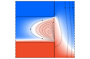
  $r_{o} = 10\ \text {mm} > r_{i}$ (
 $i$ inner and
  $o$ outer). The geometry is characterised by the aspect ratio of the liquid bridge
  $\varGamma$, the rod aspect ratio
  $\varGamma _{rod}$ and the radius ratio
  $\eta$ which are defined, respectively, as
 \begin{equation} \varGamma = \frac{d}{r_{i}}=0.66, \quad \varGamma_{rod} = \frac{d_{rod}}{r_{i}}=0.4 \quad\text{and}\quad \eta = \frac{r_{o}}{r_{i}}=4. \end{equation}
These geometry parameters are identical to those of the experimental set-up used by Romanò et al. (Reference Romanò, Kuhlmann, Ishimura and Ueno2017) and they are kept constant throughout.
The liquid bridge is made of 2-cSt silicone oil KF96L-2cs produced by Shin-Etsu Chemical (Japan), while the surrounding gas is air. Both are considered Newtonian fluids. The liquid bridge is kept in place by capillary forces due to the surface tension between the liquid and the gas and by pinning of the three-phase contact lines to the sharp circular edges of the support rods. The support rods are assumed to be perfect thermal conductors and are kept at different but constant temperatures  $T_{top} = T_0 + \Delta T/2$ and
  $T_{bottom} = T_0 - \Delta T/2$ with
  $\Delta T=T_{top}-T_{bottom}$ and
  $T_0=(T_{top}+T_{bottom})/2$. The temperature difference
  $\Delta T$ can accept positive or negative values corresponding to heating from above or from below, respectively. Since the imposed temperature difference leads to a surface tension variation along the interface, tangential interfacial stresses are induced via the thermocapillary effect. These thermocapillary stresses drive a flow both in the liquid and in the gas phase (Kuhlmann Reference Kuhlmann1999).
The dependence of the surface tension
 \begin{equation} \sigma(T)=\sigma_0-\gamma(T-T_0)+O[ (T-T_0 )^2 ] \end{equation}
on the temperature  $T$ is considered up to first order in
  $T-T_0$, where
  $\sigma _0 = \sigma (T_0)$ is the surface tension at the reference temperature
  $T_0$ and
  $\gamma$ the negative surface tension coefficient. Apart from thermocapillary surface forces, the flow is also driven by body forces caused by the thermal expansion of the liquid and the gas. Therefore, the densities
 $$\begin{gather} \rho(T) = \rho_{0} \{ 1 - \beta (T-T_0) + O[ (T-T_0 )^2 ] \}, \end{gather}$$
 $$\begin{gather}\rho_{g}(T) = \rho_{g0} \{ 1 - \beta_{g} (T-T_0 ) + O[ (T-T_0 )^2 ] \}, \end{gather}$$
of the liquid and the gas, respectively, are also considered up to first order in the temperature deviation from its algebraic mean  $T_0$, where
  $\rho _0 = \rho (T_0)$ and
  $\rho _{g0}=\rho _{g}(T_0)$ are the reference densities at the mean temperature. The respective thermal expansion coefficients are
  $\beta =-\rho _0^{-1}(\partial \rho / \partial T)_p$ and
  $\beta _{g}=-\rho _{g0}^{-1}(\partial \rho _{g} / \partial T)_p$.
A third driving force of the fluid motion is an imposed axial pressure difference between the inlet and the outlet of the gas (figure 1). The pressure difference leads to a forced flow in the annular gap between the rods and the shield tube. The direction of the mean gas flow depends on the sign of the pressure difference. Here we assume that the gas enters the annular space with a temperature equal to the rod temperature upstream of the gas flow.
For millimetric liquid bridges of the above silicone oil which can be realised under terrestrial gravity the main driving force is thermocapillarity. As long as the imposed temperature difference and the gas flow rate are small the flow in the liquid and in the gas will be axisymmetric and steady, reflecting the symmetry of the problem. Here we are interested in the stability of this steady axisymmetric flow and the dependence of its stability boundary on the forced flow in the gas phase. In order to keep this problem manageable we assume the dynamic viscosities of both fluids  $\mu$ and
  $\mu _{g}$ as well as their thermal conductivities
  $\lambda$ and
  $\lambda _{g}$ and their specific heat capacities
  $c_p$ and
  $c_{p,{g}}$ to be constant. Moreover, the mean temperature is kept constant at
  $T_0=25\,^\circ$C. All physical properties for both working fluids are given in table 1.
Table 1. Thermophysical properties of the working fluids 2-cSt silicone oil KF96L-2cs and air at  $25\,^\circ$C.

2.2. Governing equations and boundary conditions
2.2.1. Transport equations
The flow in both the liquid and the gas phase is governed by the Navier–Stokes, continuity and energy equations. For the problem at hand it seems reasonable to simplify the governing equations and consider the Oberbeck–Boussinesq approximation (Landau & Lifschitz Reference Landau and Lifschitz1959; Mihaljan Reference Mihaljan1962) which takes into account density variations only in the buoyancy term. However, a proper treatment of flow-induced deformations of the liquid–gas interface requires higher-order corrections to the Oberbeck–Boussinesq approximation (Simanovskii & Nepomnyashchy Reference Simanovskii and Nepomnyashchy1993). Therefore, we consider the linear temperature dependence of the densities not only in the buoyancy term, but also in the entire momentum equations, the continuity equations and in the energy equations for both the liquid and the gas.
Within this approximation we consider the following equations for the velocity  $\boldsymbol {u}$, pressure
  $p$ and temperature field
  $T$ for the liquid phase:
 $$\begin{gather} \rho\frac{\partial \boldsymbol{u}}{\partial t} +\rho \boldsymbol{u} \boldsymbol{\cdot} \boldsymbol{\nabla} \boldsymbol{u} ={-} \boldsymbol{\nabla} p - \rho g \boldsymbol{e}_z + \mu \boldsymbol{\nabla} \boldsymbol{\cdot} \boldsymbol{\mathsf{S}}, \end{gather}$$
 $$\begin{gather}\frac{\partial \rho}{\partial t} + \boldsymbol{\nabla} \boldsymbol{\cdot} (\rho \boldsymbol{u}) = 0, \end{gather}$$
 $$\begin{gather}\rho \frac{\partial T}{\partial t} + \rho \boldsymbol{u} \boldsymbol{\cdot} \boldsymbol{\nabla} T = \frac{\lambda}{c_p} \nabla^2 T, \end{gather}$$
where  $t$ is the time and
 \begin{equation} \boldsymbol{\mathsf{S}}=\boldsymbol{\nabla} \boldsymbol{u} + (\boldsymbol{\nabla}\boldsymbol{u})^{T} - \tfrac{2}{3}(\boldsymbol{\nabla}\boldsymbol{\cdot}\boldsymbol{u})\boldsymbol{\mathsf{I}} \end{equation}
is (twice) the deformation rate tensor with the identity matrix  ${\boldsymbol{\mathsf{I}}} = \delta _{ij}$. In the energy equation (2.4c), the pressure contribution to the enthalpy is neglected, assuming
  ${p/\rho \ll |c_p T|}$. Likewise, we neglect the pressure work and the heat due to viscous dissipation in (2.4c).
Formally the same equations (2.4) hold for the gas phase, merely with the material parameters of the gas. To distinguish between liquid and gas we follow Stojanovic et al. (Reference Stojanović, Romanò and Kuhlmann2022) and introduce the set of coefficients
 \begin{equation} \boldsymbol{\alpha} = ( \alpha_\rho,\alpha_\mu,\alpha_\lambda,\alpha_{c_p},\alpha_\beta )= \begin{cases} (1,1,1,1,1) \quad \text{for the liquid phase,}\\ (\tilde{\rho},\tilde{\mu},\tilde{\lambda},\widetilde{c_p},\tilde\beta) \quad \text{for the gas phase}, \end{cases} \end{equation}
where  $\tilde {\rho }=\rho _{g0}/\rho _0$,
  $\tilde {\mu }=\mu _{g}/\mu$,
  $\tilde {\lambda }=\lambda _{g}/\lambda$,
  $\widetilde {c_p}=c_{p,{g}}/c_p$ and
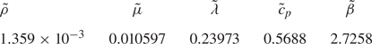
  $\tilde \beta =\beta _{g}/\beta$ denote the ratios of the reference densities, dynamic viscosities, thermal conductivities, specific heat capacities and the thermal expansion coefficients between the gas and the liquid. Numerical data are given in table 2.
Table 2. Ratios of the thermophysical parameters between air and 2-cSt silicone oil as defined in (2.6).
Scaling lengths, time, velocity, pressure and temperature by  $d$,
$d$,  $d^2\rho _0/\mu$,
  $\gamma \Delta T/\mu$,
  $\gamma \Delta T/d$ and
  $\Delta T$, respectively, and using the same notation as for the dimensional variables, we arrive at the dimensionless version of (2.4) for both fluids:
 $$\begin{gather} (1-\alpha_\beta \varepsilon\vartheta)\frac{\partial \boldsymbol{u}}{\partial t} +{Re}(1-\alpha_\beta \varepsilon\vartheta) \boldsymbol{u} \boldsymbol{\cdot} \boldsymbol{\nabla} \boldsymbol{u} ={-}\frac{1}{\alpha_\rho} \boldsymbol{\nabla} p + \alpha_\beta\,{Bd}\,\vartheta \boldsymbol{e}_z +\alpha_\mu\boldsymbol{\nabla}\boldsymbol{\cdot} \boldsymbol{\mathsf{S}}, \end{gather}$$
 $$\begin{gather}-\frac{\alpha_\beta \varepsilon}{{Re}}\frac{\partial \vartheta}{\partial t} - \alpha_\beta \varepsilon\boldsymbol{\nabla}\boldsymbol{\cdot} (\vartheta \boldsymbol{u}) + \boldsymbol{\nabla} \boldsymbol{\cdot} \boldsymbol{u} = 0, \end{gather}$$
 $$\begin{gather}(1-\alpha_\beta \varepsilon\vartheta)\frac{\partial \vartheta}{\partial t} + {Re}(1-\alpha_\beta \varepsilon\vartheta)\boldsymbol{u} \boldsymbol{\cdot} \boldsymbol{\nabla} \vartheta = \frac{\alpha_\lambda}{\alpha_{c_p}{Pr}}\nabla^2 \vartheta, \end{gather}$$
where we made use of the coefficients defined in (2.6). We use cylindrical coordinates  $(r,\varphi,z)$ centred in the middle of the liquid bridge and a polar representation of the velocity field
  $\boldsymbol {u} = u\boldsymbol {e}_r + v \boldsymbol {e}_{\varphi } + w\boldsymbol {e}_z$. In (2.7), the reduced temperature and the reduced pressure are defined as
  $\vartheta =(T-T_0)/\Delta T$ and
  $p=(d/\gamma \Delta T)(P-\rho _0 g z)$, respectively, where
  $P$ indicates the dimensional pressure. Furthermore, the temperature dependence of the density is taken into account up to linear approximation with the (small) parameter
  $\varepsilon =\beta \Delta T$ (and
  $\varepsilon _{g}=\beta _{g}\Delta T$) measuring the magnitude of the density variation in the liquid (and in the gas).
The flow in the silicone oil under terrestrial gravity is characterised by the thermocapillary Reynolds number  ${Re}$, the Prandtl number
  ${Pr}$ and the dynamic Bond number
  ${Bd}$, defined respectively as
 \begin{equation} {Re}=\frac{\rho_0\gamma \Delta T d}{\mu^2},\quad {Pr}=\frac{\mu c_p}{\lambda}=28,\quad{Bd} = \frac{\rho_0 g\beta d^2}{\gamma}=0.41. \end{equation}
Since  $\Delta T$ can accept both, positive and negative values, the thermocapillary Reynolds number
  ${Re}$, the Marangoni number
  ${Ma}={Pr}{Re}$ as well as the Rayleigh number
  ${Ra}={Bd}{Ma}$ have a sign. As most investigations of the flow in liquid bridges consider heating from above, this configuration will be associated with
  $({Re},{Ma},{Ra})>0$, while
  $({Re},{Ma},{Ra})<0$ indicates heating from below, even though this is an unusual convention for pure buoyancy convection.
2.2.2. Linear stability equations
The steady axisymmetric solution  $\boldsymbol{u}_0 = u(r,z)\boldsymbol{e}_r + w(r,z)\boldsymbol{e}_z$ of (2.7) is called the basic flow. For sufficiently small driving forces the basic flow is stable. We are interested in the linear stability boundary of the basic flow when the thermocapillary Reynolds numbers
  ${Re}$ exceeds a certain threshold. For Reynolds numbers larger in magnitude than the critical Reynolds number, i.e.
  ${Re}>{Re}_c>0$ for heating from above, or
  ${Re}<{Re}_c<0$ for heating from below, the flow is time-dependent, three-dimensional or both. In order to find the critical Reynolds numbers
  ${Re}_c$ a linear stability analysis is carried out. To that end the general three-dimensional time-dependent solution
  $\boldsymbol {q}=(u,v,w,p,\vartheta )$ and
  $\boldsymbol {q}_{g}=(u_{g},v_{g},w_{g},p_{g},\vartheta _{g})$ of (2.7) is decomposed into an axisymmetric time-independent basic flow (subscript 0) and deviations from this basic flow (indicated by a prime
  $'$):
$'$):
 \begin{equation} \boldsymbol{q}=\boldsymbol{q}_0(r,z)+\boldsymbol{q}'(r,\varphi,z,t),\quad \boldsymbol{q}_{g}=\boldsymbol{q}_{g0}(r,z)+\boldsymbol{q}'_{g}(r,\varphi,z,t). \end{equation}
Inserting this decomposition into (2.7) and linearising the equations with respect to the perturbation quantities yields the set of linear equations
 \begin{align} &(1-\alpha_\beta \varepsilon\vartheta_0)\frac{\partial \boldsymbol{u}'}{\partial t} + {Re}(1-\alpha_\beta \varepsilon\vartheta_0)(\boldsymbol{u}_0 \boldsymbol{\cdot} \boldsymbol{\nabla} \boldsymbol{u}'+ \boldsymbol{u}' \boldsymbol{\cdot} \boldsymbol{\nabla} \boldsymbol{u}_0) - \alpha_\beta \varepsilon {Re} \vartheta' \boldsymbol{u}_0 \boldsymbol{\cdot} \boldsymbol{\nabla} \boldsymbol{u}_0 \nonumber\\ &\quad ={-}\frac{1}{\alpha_\rho}\boldsymbol{\nabla} p'+\alpha_\beta \,{Bd}\,\vartheta' \boldsymbol{e}_z +\alpha_\mu\boldsymbol{\nabla} \boldsymbol{\cdot} {\boldsymbol{\mathsf{S}}}', \end{align}
 \begin{align} &-\frac{\alpha_\beta \varepsilon}{{Re}}\frac{\partial \vartheta'}{\partial t} - \alpha_\beta \varepsilon\boldsymbol{\nabla}\boldsymbol{\cdot} (\vartheta' \boldsymbol{u}_0) - \alpha_\beta \varepsilon\boldsymbol{\nabla}\boldsymbol{\cdot} (\vartheta_0 \boldsymbol{u}') + \boldsymbol{\nabla} \boldsymbol{\cdot} \boldsymbol{u}' = 0, \end{align}
 \begin{align} &(1-\alpha_\beta \varepsilon\vartheta_0)\frac{\partial \vartheta'}{\partial t} + {Re}(1-\alpha_\beta \varepsilon\vartheta_0)(\boldsymbol{u}_0 \boldsymbol{\cdot} \boldsymbol{\nabla} \vartheta'+ \boldsymbol{u}' \boldsymbol{\cdot} \boldsymbol{\nabla} \vartheta_0) \nonumber\\ &\quad - \alpha_\beta \varepsilon {Re} \vartheta' \boldsymbol{u}_0 \boldsymbol{\cdot} \boldsymbol{\nabla} \vartheta_0 = \frac{\alpha_\lambda}{\alpha_{c_p}{Pr}}\nabla^2 \vartheta', \end{align}
which describe the dynamics of the infinitesimal perturbation flow. Again (2.10) is valid for both phases, distinguished by  $\boldsymbol{\alpha}$. Both phases are coupled through the boundary conditions on the interface.
Since the basic state is homogeneous in time  $t$ and in the azimuthal coordinate
  $\varphi$, the perturbations
  $\boldsymbol {q}'$ and
  $\boldsymbol {q}'_{g}$ can be decomposed into normal modes with azimuthal wavenumber
  $m\in \mathbb {N}$:
 \begin{equation} \boldsymbol{q}' = \sum_{j,m} \hat{\boldsymbol{q}}_{j,m}(r,z)\,{\rm e}^{\psi_{j,m} t+\mathrm{i} m\varphi}+\text{c.c.},\quad \boldsymbol{q}'_{g} = \sum_{j,m} \hat{\boldsymbol{q}}_{{g};j,m}(r,z)\,{\rm e}^{\psi_{j,m} t+\mathrm{i} m\varphi}+\text{c.c.}, \end{equation}
where the complex conjugate (c.c.) renders the perturbations real. The complex growth rates of the normal modes with amplitudes  $\hat {\boldsymbol {q}}=(\hat {u},\hat {v},\hat {w},\hat {p},\hat {\vartheta })$ and
  $\hat {\boldsymbol {q}}_{g} = (\hat {u}_{g}, \hat {v}_{g}, \hat {w}_{g}, \hat {p}_{g}, \hat {\vartheta }_{g})$ are denoted
  $\psi = \psi _{j,m} \in \mathbb {C}$, where the index
  $j$ numbers the different solutions for given wavenumber
  $m$.
$m$.
Inserting the ansatz (2.11) into (2.10), we obtain linear differential equations in  $r$ and
  $z$ for the perturbation amplitudes
 \begin{align} &\psi(\hat{u}-\alpha_\beta \varepsilon u_0 \hat{\vartheta})+{Re}\left[ \left( \frac{1}{r} +\frac{\partial }{\partial r} \right) (2u_0\hat{u}) +\frac{m u_0 \hat{\hat{v}}}{r} +\frac{\partial (u_0 \hat{w}+\hat{u}w_0)}{\partial z}\right]\nonumber\\ &\quad -\alpha_\beta \varepsilon{Re}\left[ \left( \frac{1}{r}+\frac{\partial}{\partial r} \right)(\vartheta' u_0^2)+\frac{\partial (\vartheta' u_0 w_0)}{\partial z} \right] ={-}\frac{1}{\alpha_\rho} \frac{\partial \hat{p}}{\partial r}+\alpha_\mu\left[ \frac{2}{r} \frac{\partial}{\partial r} \left( r\frac{\partial \hat{u}}{\partial r} \right)\right.\nonumber\\ &\quad -\left.(m^2+2)\frac{\hat{u}}{r^2}+m\left(\frac{1}{r}\frac{\partial}{\partial r}-\frac{3}{r^2}\right) \hat{\hat{v}}+\left(\frac{\partial}{\partial z}+\frac{\partial}{\partial r}\right)\frac{\partial u'}{\partial z} -\frac{2}{3}\alpha_\beta \varepsilon\zeta'\right], \end{align}
 \begin{align} &\psi\hat{\hat{v}}+{Re}\left[\left( \frac{2}{r} +\frac{\partial }{\partial r} \right) (u_0\hat{\hat{v}}) +\frac{\partial (\hat{\hat{v}}w_0)}{\partial z}\right] =\frac{1}{\alpha_\rho}\frac{m}{r}\hat{p}+\alpha_\mu\left[{-}m\left(\frac{3}{r^2}+\frac{\partial}{\partial r}\right) \hat{u}\right.\nonumber\\ &\quad \left.+ \frac{1}{r} \frac{\partial}{\partial r} \left( r\frac{\partial \hat{\hat{v}}}{\partial r} \right)-(2~m^2+1)\frac{\hat{\hat{v}}}{r^2}+\frac{\partial}{\partial z}\left(\frac{\partial \hat{\hat{v}}}{\partial z}-\frac{m\hat{w}}{r}\right)-\frac{2}{3}\alpha_\beta \varepsilon\zeta'\right], \end{align}
 \begin{align} &\psi(\hat{w}-\alpha_\beta \varepsilon w_0 \hat{\vartheta})+{Re}\left[\frac{1}{r} \frac{\partial [r(w_0 \hat{u}+\hat{w}u_0)]}{\partial r} +\frac{m w_0 \hat{\hat{v}}}{r} + 2\frac{\partial w_0\hat{w}}{\partial z}\right]\nonumber\\ &\quad-\alpha_\beta \varepsilon{Re}\left[ \left( \frac{1}{r}+\frac{\partial}{\partial r} \right)(\vartheta' u_0 w_0)+\frac{\partial (\vartheta' w_0^2)}{\partial z} \right]={-}\frac{1}{\alpha_\rho} \frac{\partial \hat{p}}{\partial z}+\alpha_\beta\,{Bd}\,\hat{\vartheta}\nonumber\\ &\quad+\alpha_\mu\left[ \frac{1}{r} \frac{\partial}{\partial r} \left( r\frac{\partial \hat{w}}{\partial r} \right)-m^2\frac{\hat{w}}{r^2}+\frac{\partial}{\partial z}\left( \frac{1}{r}\frac{\hat{u}}{\partial r}+\frac{1}{r}\hat{\hat{v}}+2\frac{\partial \hat{w}}{\partial z} \right)-\frac{2}{3}\alpha_\beta \varepsilon\zeta' \right], \end{align}
 \begin{align} &\alpha_\beta \varepsilon\left[-\frac{\psi \hat{\vartheta}}{{Re}} - \frac{1}{r}\frac{\partial (r\hat{\vartheta}u_0)}{\partial r} - \frac{\partial (\hat{\vartheta}w_0)}{\partial z}\right] + \frac{1}{r} \frac{\partial [(1-\alpha_\beta \varepsilon\vartheta_0)r \hat{u}]}{\partial r}\nonumber\\ &\quad +\frac{m-\alpha_\beta \varepsilon\vartheta_0}{r}\hat{\hat{v}}+\frac{\partial[(1-\alpha_\beta \varepsilon\vartheta_0) \hat{w}]}{\partial z}=0, \end{align}
 \begin{align} &\psi(\hat{\vartheta}-\alpha_\beta \varepsilon\vartheta_0)+{Re}\left[\frac{1}{r} \frac{\partial [r(\vartheta_0 \hat{u}+\hat{\vartheta}u_0-\alpha_\beta \varepsilon\vartheta_0 u_0 \hat{\vartheta})]}{\partial r} +\frac{m \vartheta_0 \hat{\hat{v}}}{r} \right.\nonumber\\ &\quad \left. +\frac{\partial ( \vartheta_0\hat{w}+\hat{\vartheta}w_0-\alpha_\beta \varepsilon\vartheta_0 w_0 \hat{\vartheta})}{\partial z}\right]=\frac{\alpha_\lambda}{\alpha_{c_p}{Pr}}\left[ \frac{1}{r} \frac{\partial}{\partial r} \left( r\frac{\partial \hat{\vartheta}}{\partial r} \right)-m^2\frac{\hat{\vartheta}}{r^2}+\frac{\partial^2 \hat{\vartheta}}{\partial z^2}\right]. \end{align}
In these equations, the amplitudes of the azimuthal velocities have been transformed according to  $\hat {\hat {v}}=\mathrm {i} \hat {v}$ and
  $\hat {\hat {v}}_{g}=\mathrm {i} \hat {v}_{g}$ in order to render the coefficient matrix real and, thus, save computational memory for the numerical solution (Theofilis Reference Theofilis2003). For the sake of brevity, we have abbreviated the term
  $\boldsymbol {\nabla }\boldsymbol{\cdot}\boldsymbol {u}'$ arising in the rate-of-strain tensor for the perturbation flow by
  $\boldsymbol {\nabla }\boldsymbol{\cdot}\boldsymbol {u}'=\alpha _\beta \varepsilon \zeta '$. These terms represent the deviation from a solenoidal perturbation flow. As can be seen from (2.10b) they are of the orders of
  $O(\varepsilon )$ and
  $O(\varepsilon _{g})$ for the liquid and gas phase, respectively.
2.2.3. Boundary conditions
To solve the two-dimensional version of (2.7) for the basic flow and of (2.12) for the three-dimensional perturbation flow suitable boundary conditions must be defined for both flows.
Solid walls. The velocity fields must satisfy the no-slip boundary conditions
 \begin{equation}
\boldsymbol{u}_0=\boldsymbol{u}_{g0} = 0
\quad\text{and}\quad
\hat{\boldsymbol{u}}=\hat{\boldsymbol{u}}_{g} =
0
\end{equation}
\begin{equation}
\boldsymbol{u}_0=\boldsymbol{u}_{g0} = 0
\quad\text{and}\quad
\hat{\boldsymbol{u}}=\hat{\boldsymbol{u}}_{g} =
0
\end{equation}on all solid walls, namely the support rods and the cylindrical tube confining the gas radially. Since the support rods are always made from good thermal conductors (e.g. Romanò et al. Reference Romanò, Kuhlmann, Ishimura and Ueno2017; Gotoda et al. Reference Gotoda, Toyama, Ishimura, Sano, Suzuki, Kaneko and Ueno2019), constant temperatures are imposed on the rods for the basic flow, while the perturbation temperature must vanish. The shield tube, on the other hand, is typically made from a good thermal insulator to keep its thermal effect on the gas flow at a minimum. Therefore, the heat fluxes due to both the basic and the perturbation temperature field are required to vanish on the shield tube. This leads to the thermal boundary conditions
 $$\begin{gather} \text{hot rod: } \quad \vartheta_0=\vartheta_{g0}= 1/2 \quad \text{and} \quad \hat{\vartheta}=\hat{\vartheta}_{g} = 0, \end{gather}$$
 $$\begin{gather}\text{cold rod: } \quad \vartheta_0=\vartheta_{g0}={-}1/2 \quad \text{and} \quad \hat{\vartheta}=\hat{\vartheta}_{g} = 0, \end{gather}$$
 $$\begin{gather}\text{shield tube: } \quad \partial \vartheta_{g0} / \partial r =0 \quad \text{and} \quad \partial \hat{\vartheta}_{g} / \partial r =0. \end{gather}$$
 Axis of symmetry. On the axis of symmetry at  $r=0$ the axisymmetric steady basic flow must satisfy
 \begin{equation} u_0=\frac{\partial w_0}{\partial r}=\frac{\partial \vartheta_0}{\partial r}=0. \end{equation}
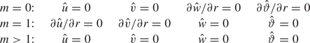
The boundary conditions for the perturbation flow can be derived from uniqueness conditions for  $\partial u/\partial \varphi$ and
  $\partial \vartheta /\partial \varphi$ as
  $r\to 0$ (see also Batchelor & Gill Reference Batchelor and Gill1962; Xu & Davis Reference Xu and Davis1984) and depend on the wavenumber
  $m$. They are given in table 3.
Table 3. Boundary conditions for the perturbation flow on  $r=0$.
Liquid–gas interface. The flow in the liquid and in the gas phase are coupled through the interface. Since the location of the interface, described by  $r=h(\varphi,z,t)$, is part of the solution, the flow and the location
  $h$ must be computed in a coupled manner. In the following we consider the axisymmetric steady basic flow and the corresponding time-independent shape function
  $h_0(z)$.
Regardless of the shape of the interface, continuity of the temperature and of the heat flux across the interface at  $r=h_0(z)$ require the thermal boundary conditions
 $$\begin{gather} r=h_0:\quad \vartheta_0 = \vartheta_{g0}, \end{gather}$$
 $$\begin{gather}r=h_0:\quad \boldsymbol{n}\boldsymbol{\cdot} \boldsymbol{\nabla} \vartheta_0 = \tilde{\lambda}\boldsymbol{n}\boldsymbol{\cdot} \boldsymbol{\nabla} \vartheta_{g0} , \end{gather}$$
where
 \begin{equation} \boldsymbol{n} = \frac{\boldsymbol{e}_r - (\partial_z h_0)\boldsymbol{e}_z}{N}, \quad \text{with}\ N=\sqrt{1+(\partial_z h_0)^2}, \end{equation}
is the unit vector on the interface directed from the liquid into the gas. The tangent vector is defined as  $\boldsymbol{t} = [(\partial _z h_0)\boldsymbol{e}_r +\boldsymbol{e}_z]/N$.
The velocity fields must satisfy kinematic and dynamic boundary conditions. The kinematic boundary conditions
 \begin{equation} r=h_0: \quad \boldsymbol{u}_0 = \boldsymbol{u}_{g0} \quad \text{and} \quad \frac{u_0}{w_0} = \partial_z h_0 \end{equation}
ensure the continuity of the velocity and guarantee that a fluid element on the interface remains on the interface. The dynamic boundary condition is decomposed into a normal and a tangential stress balance by projecting the equilibrium of forces onto the normal ( $\boldsymbol{n}$) and tangential (
 $\boldsymbol{t}$) directions. The normal stress balance
 \begin{align} &-(p_0-p_{g0}) +
\boldsymbol{n} \boldsymbol{\cdot} {\boldsymbol{\mathsf{S}}}_0
\boldsymbol{\cdot} \boldsymbol{n} + \left( \frac{1}{{Ca}}
-\vartheta_0\right)
\boldsymbol{\nabla}\boldsymbol{\cdot}\boldsymbol{n}\nonumber\\
&\quad
={-}\frac{{Bo}}{{Ca}}z-(\vartheta-\tilde{\rho}\tilde{\beta}\vartheta_{g0})\,{Bd}\,
z+\tilde{\mu}\boldsymbol{n} \boldsymbol{\cdot}
\boldsymbol{\mathsf{S}}_{g0} \boldsymbol{\cdot} \boldsymbol{n}
\end{align}
\begin{align} &-(p_0-p_{g0}) +
\boldsymbol{n} \boldsymbol{\cdot} {\boldsymbol{\mathsf{S}}}_0
\boldsymbol{\cdot} \boldsymbol{n} + \left( \frac{1}{{Ca}}
-\vartheta_0\right)
\boldsymbol{\nabla}\boldsymbol{\cdot}\boldsymbol{n}\nonumber\\
&\quad
={-}\frac{{Bo}}{{Ca}}z-(\vartheta-\tilde{\rho}\tilde{\beta}\vartheta_{g0})\,{Bd}\,
z+\tilde{\mu}\boldsymbol{n} \boldsymbol{\cdot}
\boldsymbol{\mathsf{S}}_{g0} \boldsymbol{\cdot} \boldsymbol{n}
\end{align}
must be satisfied on  $r=h_0(z)$. It is affected by the static Bond number
  ${Bo}$ and the Capillary number
  ${Ca}$ defined as
 \begin{equation} {Bo} = \frac{(\rho_0-\rho_{g0}) g d^2}{\sigma_0},\quad {Ca} = \frac{\gamma\Delta T}{\sigma_0}. \end{equation}
They measure the relative importance of static and of hydrodynamic pressure differences, respectively, to the characteristic capillary pressure  $\sigma _0/d$. Note that the ratio
  $\tau ={Bd}/{Bo} = \rho _0\beta \sigma _0 / [\gamma (\rho _0-\rho _{g0})]$ is a material constant and almost a proportionality factor between
  $\varepsilon$ and
  ${Ca}$, since
  $\varepsilon =(1-\tilde {\rho })\tau {Ca}$ and typically
  $\tilde {\rho }\ll 1$. In addition to (2.19) the tangential stress balance
 \begin{equation} \boldsymbol{t}\boldsymbol{\cdot}\boldsymbol{\mathsf{S}}_0\boldsymbol{\cdot}\boldsymbol{n} ={-}\boldsymbol{t} \boldsymbol{\cdot} \boldsymbol{\nabla} \vartheta_0 +\tilde{\mu} \boldsymbol{t}\boldsymbol{\cdot}\boldsymbol{\mathsf{S}}_{g0}\boldsymbol{\cdot}\boldsymbol{n} \end{equation}
must also hold on  $r=h_0(z)$. The thermocapillary stresses are represented by
  $-\boldsymbol{t}\boldsymbol{\cdot}\boldsymbol {\nabla } \vartheta _0$.
The stationary axisymmetric version of the differential equations (2.7) and the above boundary conditions for the basic state must be solved in a coupled way to yield the basic flow including the interfacial shape  $h_0(z)$. The numerical solution is described in § 3. To be able to solve the problem two additional constraints for
  $h_0$ are required, because the normal stress balance is of second order in
  $z$. These are provided by the interface
  $h_0(z=\pm 1/2 ) = 1/\varGamma$ being pinned to the sharp edges of the heated rods. In addition, for a non-volatile liquid the mass of the liquid bridge must be conserved. Since 2-cSt silicone oil is slightly volatile, accurate experiments (e.g. Yano et al. Reference Yano, Maruyama, Matsunaga and Nishino2016; Yasnou et al. Reference Yasnou, Gaponenko, Mialdun and Shevtsova2018; Gotoda et al. Reference Gotoda, Toyama, Ishimura, Sano, Suzuki, Kaneko and Ueno2019) control the volume of the liquid rather than the mass. Therefore, we impose the volume constraint
 \begin{equation} \varGamma^2\int_{{-}1/2}^{1/2} h_0^2(z)\,\mathrm{d} z={\mathcal{V}}, \end{equation}
where  ${\mathcal {V}}=V_l/V_0$ is the liquid volume
  $V_l$ normalised by the volume
  $V_0={\rm \pi} r_{i}^2 d$ of an upright cylindrical liquid bridge. Throughout this investigation the liquid volume
  ${\mathcal {V}}$ is prescribed, not the mass of the liquid
  $M = \int _{V_l} \rho (\boldsymbol{x}) \,\mathrm{d} V$.
In order to identify the flow-induced contribution to the surface shape resulting from (2.19), and of its effect on the flow stability, we also consider the hydrostatic case ( ${\boldsymbol{u}_0=\boldsymbol{u}_{g,0}=0}$) in which (2.19) becomes the Young–Laplace equation
 \begin{equation} \Delta p_h = \frac{\boldsymbol{\nabla} \boldsymbol{\cdot} \boldsymbol{n}}{{Ca}} +\frac{{Bo}}{{Ca}} z, \end{equation}
where  $\Delta p_h$ is a constant overpressure (Kuhlmann Reference Kuhlmann1999). The resulting static surface shape is denoted
  $h_{0,s}$ (subscript
  $s$ denoting static). As long as the effect of the flow on the shape of the interface is weak,
  $h_{0,s}$ represents a good approximation to the true dynamic surface shape
  $h_{0,d}$ (subscript
  $d$ denoting dynamic) which results from (2.19). To assess the influence of the flow on the shape of the interface we define the dynamic surface deformation
  $\Delta h_0 = h_{0,d} - h_{0,s}$ as the difference between both surface shapes. Similarly,
  ${Re}_{c,s}$ and
  ${Re}_{c,d}$ denote the critical Reynolds numbers assuming a static or a dynamic interfacial shape, respectively, for the basic flow.
Finally, interfacial coupling conditions must be provided for the perturbation flow. To reduce the computational effort, and motivated by the results of Carrión et al. (Reference Carrión, Herrada and Montanero2020), we neglect interfacial deformations due to the perturbation flow. In this approach, the interfacial conditions
 \begin{equation} \left.\begin{array}{c}
\hat{\boldsymbol{u}}=\hat{\boldsymbol{u}}_{g},\quad
\hat{\vartheta} = \hat{\vartheta}_{g}, \quad
\boldsymbol{n}\boldsymbol{\cdot} \boldsymbol{\nabla}
\hat{\vartheta} = \tilde{\lambda}
\boldsymbol{n}\boldsymbol{\cdot} \boldsymbol{\nabla}
\hat{\vartheta}_{g},\\ \text{and} \quad
\boldsymbol{t}\boldsymbol{\cdot}\hat{{\boldsymbol{\mathsf{S}}}}\boldsymbol{\cdot}\boldsymbol{n}
={-}\boldsymbol{t}\boldsymbol{\cdot}\boldsymbol{\nabla}
\hat{\vartheta} +\tilde{\mu}
\boldsymbol{t}\boldsymbol{\cdot}\hat{{\boldsymbol{\mathsf{S}}}}_{g}\boldsymbol{\cdot}\boldsymbol{n},
\end{array}\right\} \end{equation}
\begin{equation} \left.\begin{array}{c}
\hat{\boldsymbol{u}}=\hat{\boldsymbol{u}}_{g},\quad
\hat{\vartheta} = \hat{\vartheta}_{g}, \quad
\boldsymbol{n}\boldsymbol{\cdot} \boldsymbol{\nabla}
\hat{\vartheta} = \tilde{\lambda}
\boldsymbol{n}\boldsymbol{\cdot} \boldsymbol{\nabla}
\hat{\vartheta}_{g},\\ \text{and} \quad
\boldsymbol{t}\boldsymbol{\cdot}\hat{{\boldsymbol{\mathsf{S}}}}\boldsymbol{\cdot}\boldsymbol{n}
={-}\boldsymbol{t}\boldsymbol{\cdot}\boldsymbol{\nabla}
\hat{\vartheta} +\tilde{\mu}
\boldsymbol{t}\boldsymbol{\cdot}\hat{{\boldsymbol{\mathsf{S}}}}_{g}\boldsymbol{\cdot}\boldsymbol{n},
\end{array}\right\} \end{equation}
where  $\hat{\boldsymbol{\mathsf{S}}}=\boldsymbol {\nabla } \hat {\boldsymbol {u}} + (\boldsymbol {\nabla }\hat {\boldsymbol {u}})^{\textrm {T}} - 2/3(\boldsymbol {\nabla }\boldsymbol{\cdot}\hat {\boldsymbol {u}}){\boldsymbol{\mathsf{I}}}$, are imposed at
  $r=h_0(z)$. This approximation a priori precludes surface-wave instabilities which could possibly be triggered by the shear flow due to thermocapillary and/or mechanical stresses from the gas phase. However, such surface-wave instabilities have not yet been observed experimentally in the present flow system.
Inlet and outlet. The gas enters the annular duct through the inlet located at  $z=z_{in}$ with a dimensional mean inlet velocity
  $\bar w_{g,in}$. It leaves the chamber through the outlet at
  $z=z_{out}$ on the opposite side. The oriented mean value
  $\bar w_{g,in}$ can be either positive or negative depending on the direction of the through flow. To measure the intensity of the gas flow we define the gas flow Reynolds number
 \begin{equation} {Re}_{g} = \frac{\rho_0 \bar w_{g,in} d}{\mu}. \end{equation}
It can take positive and negative values. The Reynolds number (2.25) describes the forcing of the liquid flow due to the gas motion. As shown in Appendix A,  ${Re}_{g}$ is better suited to correlate the effect of the gas motion on the liquid phase than the conventional Reynolds number
  ${Re}_{g}'$ based on the gap width
  $r_{o}-r_{i}$ and the kinematic viscosity of the gas
  $\mu _{g}/\rho _{g0}$.
For  ${Re}_{g} > 0$ (
 ${Re}_{g} < 0$) the forced flow is directed in positive (negative)
  $z$ direction. Accordingly, the locations of the inlet and the outlet
 \begin{equation} z_{in}={\pm}(1/2+\varGamma_{rod}/\varGamma) ={-}z_{out} \quad \text{for}\ {Re}_{g} \lessgtr 0 \end{equation}
are determined by the sign of  ${Re}_{g}$. To avoid entrance-length effects we assume a fully developed annular Poiseuille flow at
  $z=z_{in}$:
 \begin{equation} \boldsymbol{u}_{g0}(r) =\frac{{Re}_{g}}{{Re}}\frac{2 \ln (\eta)}{(\eta^2+1 ) \ln (\eta) -\eta^2+1}\left[1-\varGamma^2 r^2+ ( \eta^2-1 )\frac{\ln (\varGamma r)}{\ln (\eta)} \right]\boldsymbol{e}_z, \end{equation}
where the factor  ${Re}^{-1}$ arises due to the scaling. At the outlet
  $z=z_{out}$, kinematic outflow conditions
 \begin{equation} \frac{\partial u_{g0}}{\partial z}=\frac{\partial v_{g0}}{\partial z}=\frac{\partial w_{g0}}{\partial z}=0 \end{equation}
are imposed. Since the in- and outflow boundaries in a planned space experiment are realised by thermally conducting metallic porous media in contact with the support cylinders (S. Matsumoto, private communication), the gas enters/leaves the chamber with a homogeneous temperature
 \begin{equation} z={\pm} (1/2+\varGamma_{rod}/\varGamma) : \quad \vartheta_{g0}={\pm} 1/2\,\text{sgn}({Re}), \end{equation}
corresponding to the temperature of the rod next to the inlet/outlet. In the limit  ${Re}_{g} \uparrow \downarrow 0$ (2.27) and (2.28) are replaced by rigid boundary conditions.
Since the in- and outflow conditions are taken care of by the basic flow, the amplitudes of the perturbation flow must satisfy the homogeneous conditions
 $$\begin{gather} z=z_{in}: \quad \hat{u}_{g}=\hat{v}_{g}=\hat{w}_{g}=\hat{\vartheta}_{g}=0, \end{gather}$$
 $$\begin{gather}z=z_{out}: \quad \partial \hat{u}_{g}/\partial z=\partial\hat{v}_{g}/\partial z=\partial\hat{w}_{g}/\partial z=\hat{\vartheta}_{g}=0. \end{gather}$$
2.3. Energetics
The instability mechanism is investigated by the a posteriori energy analysis of the perturbation flow (Wanschura et al. Reference Wanschura, Shevtsova, Kuhlmann and Rath1995). The equations for the rates of change of the normalised kinetic and thermal perturbation energies in the liquid and in the gas phase
 $$\begin{gather} \frac{\mathrm{d} E_{kin}}{\mathrm{d} t} = \frac{1}{{\mathcal{D}}_{kin}}\frac{\mathrm{d}}{\mathrm{d} t}\int_{V_i} \frac{{\boldsymbol{u}'}^2}{2} \,\mathrm{d} V ={-}1+ M_r + M_\varphi + M_z + \sum_{j=1}^5 I_j + B + K_{g} + \varLambda_\rho , \end{gather}$$
 $$\begin{gather}\frac{\mathrm{d} E_{th}}{\mathrm{d} t} = \frac{1}{{\mathcal{D}}_{th}} \frac{\mathrm{d}}{\mathrm{d} t} \int_{V_i} \frac{{\vartheta'}^2}{2} \,\mathrm{d} V ={-}1 + \sum_{j=1}^2 J_j + H_{fs} + K_{th,g} + \varPi_\rho\end{gather}$$
can be derived by multiplying (2.10a) and (2.10c) with  $\boldsymbol {u}'$ and
  $\vartheta '$, respectively, integrating separately over the volume occupied by the liquid and by the gas, and normalising by the dissipation
  ${\mathcal {D}}_{kin}$ and
  ${\mathcal {D}}_{th}$, respectively. Detailed expressions and descriptions of all terms appearing in (2.31) can be found in Stojanovic et al. (Reference Stojanović, Romanò and Kuhlmann2022), who used the same notation. For a derivation of (2.31) for a full temperature dependence of all thermophysical parameters, we refer to Stojanović, Romanò & Kuhlmann (Reference Stojanović, Romanò and Kuhlmann2023a). For the sake of completeness the individual terms are reproduced explicitly here. The kinetic energy budget contains the following terms which are identical with the ones known from the Oberbeck–Boussinesq approximation (Nienhüser & Kuhlmann Reference Nienhüser and Kuhlmann2002):
 $$\begin{gather} {\mathcal{D}}_{kin} = \alpha_\mu \int_{V_i} (\boldsymbol{\nabla} \times \boldsymbol{u}')^2\, \mathrm{d} V \pm 8{\rm \pi}\alpha_\mu \int_{{-}1/2}^{1/2} ( h_0 (\partial_{zz} h_0) \hat{w}^2 - \hat{v}^2 )\,\mathrm{d} z, \end{gather}$$
 $$\begin{gather}\sum_{j=1}^5 I_j ={-}\frac{{Re}}{{\mathcal{D}}_{kin}} \int_{V_i} \left( v'^2\frac{u_0}{r} + u'^2\frac{\partial u_0}{\partial r} + u'w' \frac{\partial u_0}{\partial z} + u'w' \frac{\partial w_0}{\partial r} + w'^2\frac{\partial w_0}{\partial z} \right) \mathrm{d} V, \end{gather}$$
 $$\begin{gather}M_r={\pm} \frac{4{\rm \pi}\alpha_\mu}{{\mathcal{D}}_{kin}} \int_{{-}1/2}^{1/2} h_0 (\partial_z h_0) \hat{u} \left( \frac{\partial \hat{w}}{\partial r} - \frac{\partial \hat{u}}{\partial z} \right) \mathrm{d} z, \end{gather}$$
 $$\begin{gather}M_\varphi ={\pm} \frac{4{\rm \pi}\alpha_\mu}{{\mathcal{D}}_{kin}} \int_{{-}1/2}^{1/2} h_0 \hat{v} \left( \frac{\partial \hat{v}}{\partial r} - \frac{\hat{v}^2}{h_0} - (\partial_z h_0) \frac{\partial \hat{v}}{\partial z} \right) \mathrm{d} z, \end{gather}$$
 $$\begin{gather}M_z ={\pm} \frac{4{\rm \pi}\alpha_\mu}{{\mathcal{D}}_{kin}} \int_{{-}1/2}^{1/2} h_0 \hat{w} \left( \frac{\partial \hat{w}}{\partial r} + (\partial_z h_0) \hat{w} - (\partial_z h_0) \frac{\partial \hat{w}}{\partial z} \right) \mathrm{d} z, \end{gather}$$
 $$\begin{gather}B = \frac{\alpha_\beta\,{Bd}}{{\mathcal{D}}_{kin}} \int_{V_i} w'\vartheta' \, \mathrm{d} V, \end{gather}$$
where the volume integrals are evaluated in both volumes, occupied by the liquid and the gas, respectively, i.e.  $i \in [\textrm {l}, \textrm {g}]$. Due to the opposing orientations of the normal vectors for the liquid and the gas, the surface integrals carry different signs, where the upper (lower) sign applies to the liquid (gas) phase. The terms
  $I_j$ describe inertial processes, while
  $M_r$,
  $M_\varphi$ and
  $M_z$ represent kinetic energy production terms due to thermocapillary forces caused by the perturbation flow, and
  $B$ represents the energy production rate due to buoyancy forces.
The terms entering the thermal energy budget in the framework of the Oberbeck–Boussinesq approximation are
 $$\begin{gather} {\mathcal{D}}_{th} = \frac{\alpha_\lambda}{\alpha_{cp}{Pr}} \int_{V_i} (\boldsymbol{\nabla} \vartheta')^2 \, \mathrm{d} V, \end{gather}$$
 $$\begin{gather}\sum_{j=1}^2 J_j ={-}\frac{{Re}}{{\mathcal{D}}_{th}} \int_{V_i} \vartheta' \left( u' \frac{\partial \vartheta_0}{\partial r} + w'\frac{\partial \vartheta_0}{\partial z} \right) \mathrm{d} V, \end{gather}$$
 $$\begin{gather}H_{fs} ={\pm} \frac{2{\rm \pi}\alpha_\lambda}{\alpha_{cp}{\mathcal{D}}_{th} {Pr}}\int_{{-}1/2}^{1/2} h_0 \left( \frac{\partial \hat{\vartheta}^2}{\partial r} - (\partial_z h_0) \frac{\partial \hat{\vartheta}^2}{\partial z} \right) \mathrm{d} z. \end{gather}$$
Here, the terms  $J_j$ abbreviate the production rates of thermal energy by advection of basic state temperature caused by the perturbation flow and
  $H_{fs}$ represents the rate of heat loss/gain by the heat flux through the free surface due to the perturbation flow.
When the linear temperature dependence of the densities is considered in the entire governing equations, the terms
 \begin{align} \varLambda_\rho &={-}\alpha_\beta \varepsilon\frac{{Re}}{2{\mathcal{D}}_{kin}}\int_{V_i}\vartheta'\boldsymbol{u}'\boldsymbol{\cdot}(\boldsymbol{u}_0\boldsymbol{\cdot}\boldsymbol{\nabla}\boldsymbol{u}_0)\,\mathrm{d} V+\alpha_\beta \varepsilon\frac{1}{{\mathcal{D}}_{kin}}\int_{V_i}p'\zeta'\,\mathrm{d} V\nonumber\\ &\quad -(\alpha_\beta \varepsilon)^2\frac{1}{3{\mathcal{D}}_{kin}}\int_{V_i}\zeta'^2\,\mathrm{d} V, \end{align}
 \begin{align} \varPi_\rho &={-}\alpha_\beta \varepsilon\frac{{Re}}{{\mathcal{D}}_{th}}\int_{V_i}\vartheta_0\boldsymbol{u}_0\boldsymbol{\cdot}\boldsymbol{\nabla}\vartheta'^2\,\mathrm{d} V-(\alpha_\beta \varepsilon)^2\frac{{Re}}{2{\mathcal{D}}_{th}}\int_{V_i}\vartheta'^2\boldsymbol{u}_0\boldsymbol{\cdot}\boldsymbol{\nabla}\vartheta_0^2\,\mathrm{d} V \end{align}
arise in addition to (2.32) and (2.33). The expressions  $\varLambda _\rho$ and
  $\varPi _\rho$ describe non-Oberbeck–Boussinesq effects and represent the rates of change of kinetic and thermal perturbation energy, respectively, caused by the non-uniform density distribution in the weakly compressible flow. Both terms are of the order of
  $O(\alpha _\beta \varepsilon )$ and small compared with the other
  $O(1)$ terms in (2.31). In the presence of an external gas flow, the additional terms
 $$\begin{gather} K_{g} ={-}\frac{2{\rm \pi}{Re}}{{\mathcal{D}}_{kin}}\int_{1/\varGamma}^{\eta/\varGamma}\hat{w}_{g}^2(z_{out}) w_{g0}(z_{out})\,\mathrm{d} r, \end{gather}$$
 $$\begin{gather}K_{th,g} ={-}\frac{2{\rm \pi}{Re}}{{\mathcal{D}}_{kin}}\int_{1/\varGamma}^{\eta/\varGamma}\hat{\vartheta}_{g}^2(z_{out}) w_{g0}(z_{out})\,\mathrm{d} r \end{gather}$$
appear in the kinetic and thermal energy budget, respectively. For open gas tubes,  $K_{g}$ represents the loss of kinetic energy of the perturbation flow by transport out of the gas domain. For a closed gas container (
 ${Re}_{g}=0$),
  $K_{g} = 0$ vanishes. Similarly,
  $K_{th,g}$ can only be non-zero for open gas tubes. However, owing to the prescribed temperatures at the in- and outlet,
  $\hat {\vartheta }_{g}(z_{out})=0$ (2.30). Thus,
  $K_{th,g}=0$ vanishes also for open gas tubes.
To monitor the conservation of perturbation energy, we consider the normalised residuals of the kinetic and thermal energy balances as given in Nienhüser & Kuhlmann (Reference Nienhüser and Kuhlmann2002), supplemented with the new terms:
 $$\begin{gather} \delta E_{kin} :=\left| -\frac{\mathrm{d} E_{kin}}{\mathrm{d} t}-1+ M_r + M_\varphi + M_z + \sum_{j=1}^5 I_j + B + \varLambda_\rho + K_{g} \right|, \end{gather}$$
 $$\begin{gather}\delta E_{th} :=\left| -\frac{\mathrm{d} E_{th}}{\mathrm{d} t} -1 + \sum_{j=1}^2 J_j + H_{fs} + \varPi_\rho \right|. \end{gather}$$
Throughout, we find  $\delta E_{kin}= O(10^{-2})$ and
  $\delta E_{th}= O(10^{-3})$, signaling conservation of kinetic and thermal perturbation energy.
3. Numerical methods
3.1. Basic flow
The computation of the steady axisymmetric basic flow depends on the treatment of the liquid–gas interface (see § 2.2.3). In the simplified approach in which the shape of the liquid–gas interface is independent of the flow, the static surface shape  $h_{0,s}(z)$ is computed beforehand by solving the Young–Laplace equation (2.23). Thereafter, the volume equations are solved using finite volumes and body-fitted coordinates
  ${(\xi =r/h_0,z)}$ as described in Stojanovic et al. (Reference Stojanović, Romanò and Kuhlmann2022). In the case of flow-induced free surface deformations, the volume equations are discretised by the same method, but now the normal stress balance (2.19) is solved fully coupled to the basic flow. After each iteration the body-fitted coordinates are updated, since the transformed coordinate
  $\xi$ is based on the current surface shape.
Regardless of the treatment of the interface, the nonlinear algebraic equations resulting from the discretisation of the Navier–Stokes equations (2.7) are solved iteratively using the Newton–Raphson method. If  $\boldsymbol {q}_0^{(k)}$ is a known approximation to the solution of (2.7) at the
  $k$th iteration step, an improved approximation is
 \begin{equation} \boldsymbol{q}_0^{(k+1)} = \boldsymbol{q}_0^{(k)} + \delta \boldsymbol{q}, \end{equation}
where the increment  $\delta \boldsymbol {q}$ satisfies
 \begin{equation} \boldsymbol{J}(\boldsymbol{q}_0^{(k)})\boldsymbol{\cdot} \delta \boldsymbol{q} ={-}\boldsymbol{f}(\boldsymbol{q}_0^{(k)}), \end{equation}
with  $\boldsymbol {J}(\boldsymbol {q}_0^{(k)})$ being the Jacobian operator and
  $\boldsymbol {f}(\boldsymbol {q}_0^{(k)})$ the nonlinear residual of the Navier–Stokes equations. Equation (3.2) is obtained by inserting the ansatz (3.1) into the steady axisymmetric version of (2.7) and linearising with respect to
  $\delta \boldsymbol{q}$. We obtain
 \begin{align} &{Re} (1-\alpha_\beta \varepsilon \vartheta_0^{(k)}) (\delta \boldsymbol{u} \boldsymbol{\cdot} \boldsymbol{\nabla} \boldsymbol{u}_0^{(k)} + \boldsymbol{u}_0^{(k)} \boldsymbol{\cdot} \boldsymbol{\nabla} \delta \boldsymbol{u}) - \alpha_\beta \varepsilon{Re} \boldsymbol{u}_0^{(k)} \boldsymbol{\cdot} \boldsymbol{\nabla} \boldsymbol{u}_0^{(k)}\delta \vartheta + \frac{1}{\alpha_\rho} \boldsymbol{\nabla} \delta p\nonumber\\ &\quad - \alpha_\beta \,{Bd}\; \delta \vartheta \boldsymbol{e}_z - \alpha_\mu \boldsymbol{\nabla} \delta {\boldsymbol{\mathsf{S}}} ={-}{Re} (1-\alpha_\beta \varepsilon \vartheta_0^{(k)}) \boldsymbol{u}_0^{(k)} \boldsymbol{\cdot} \boldsymbol{\nabla} \boldsymbol{u}_0^{(k)}\nonumber\\ &\quad -\frac{1}{\alpha_\rho} \boldsymbol{\nabla} p_0^{(k)} + \alpha_\beta\,{Bd}\, \vartheta_0^{(k)} \boldsymbol{e}_z + \alpha_\mu \boldsymbol{\nabla} {\boldsymbol{\mathsf{S}}}_0^{(k)}, \end{align}
 \begin{align} &\boldsymbol{\nabla} \boldsymbol{\cdot} \delta \boldsymbol{u}-\alpha_\beta \varepsilon\boldsymbol{\nabla}\boldsymbol{\cdot} (\boldsymbol{u}_0^{(k)}\delta \vartheta )-\alpha_\beta \varepsilon\boldsymbol{\nabla}\boldsymbol{\cdot} ( \vartheta_0^{(k)} \delta\boldsymbol{u}) ={-}\boldsymbol{\nabla} \boldsymbol{\cdot} \boldsymbol{u}_0^{(k)} + \alpha_\beta \varepsilon\boldsymbol{\nabla}\boldsymbol{\cdot} ( \vartheta_0^{(k)} \boldsymbol{u}_0^{(k)}),\nonumber\\ &(1-\alpha_\beta \varepsilon \vartheta_0^{(k)})(\delta \boldsymbol{u} \boldsymbol{\cdot} \boldsymbol{\nabla} \vartheta_0^{(k)} + \boldsymbol{u}_0^{(k)} \boldsymbol{\cdot} \boldsymbol{\nabla} \delta \vartheta)-\alpha_\beta \varepsilon \boldsymbol{u}_0^{(k)} \boldsymbol{\cdot} \boldsymbol{\nabla} \vartheta_0^{(k)}\delta\vartheta - \frac{\alpha_\lambda}{\alpha_{c_p}\,{Ma}} \nabla^2 \delta \vartheta \end{align}
 \begin{align} &\quad ={-}(1-\alpha_\beta \varepsilon \vartheta_0^{(k)})\boldsymbol{u}_0^{(k)} \boldsymbol{\cdot} \boldsymbol{\nabla} \vartheta^{(k)} + \frac{\alpha_\lambda}{\alpha_{c_p}\,{Ma}} \nabla^2 \vartheta^{(k)}. \end{align}
In the case of dynamic surface deformations the general solution vector of the basic flow  $\boldsymbol {q}_0=(u_0,0,w_0,p_0,\vartheta _0,h_0)$ also contains the free surface shape
  $h_0$. Therefore, the linearised version of the normal stress balance (2.19)
 \begin{align} &-(\delta p-\delta p_{g})
+ \boldsymbol{n}^{(k)} \boldsymbol{\cdot} \delta
{\boldsymbol{\mathsf{S}}} \boldsymbol{\cdot} \boldsymbol{n}^{(k)} +
\boldsymbol{n}^{(k)} \boldsymbol{\cdot}
{\boldsymbol{\mathsf{S}}}_0^{(k)} \boldsymbol{\cdot} \delta
\boldsymbol{n} + \delta \boldsymbol{n} \boldsymbol{\cdot}
{\boldsymbol{\mathsf{S}}}_0^{(k)} \boldsymbol{\cdot}
\boldsymbol{n}^{(k)}\nonumber\\
&\quad + \left(\frac{1}{{Ca}} -\vartheta_0^{(k)}\right)
\boldsymbol{\nabla}\boldsymbol{\cdot}\delta\boldsymbol{n}-\boldsymbol{\nabla}\boldsymbol{\cdot}\boldsymbol{n}^{(k)}\delta\vartheta
+ (\delta\vartheta-\tilde{\rho}\tilde{\beta}\delta\vartheta_{g})\,{Bd} \,z\nonumber\\
&\quad-\tilde{\mu}(\boldsymbol{n}^{(k)}
\boldsymbol{\cdot} \delta{\boldsymbol{\mathsf{S}}}_{g}
\boldsymbol{\cdot} \boldsymbol{n}^{(k)} +
\boldsymbol{n}^{(k)} \boldsymbol{\cdot} {\boldsymbol{\mathsf{S}}}_{g0}
\boldsymbol{\cdot} \delta\boldsymbol{n} +
\delta\boldsymbol{n} \boldsymbol{\cdot} {\boldsymbol{\mathsf{S}}}_{g0}
\boldsymbol{\cdot} \boldsymbol{n}^{(k)} )\nonumber\\
&\qquad =p_0^{(k)}- p_{g0}^{(k)}- \boldsymbol{n}^{(k)} \boldsymbol{\cdot}
{\boldsymbol{\mathsf{S}}}_0^{(k)} \boldsymbol{\cdot}
\boldsymbol{n}^{(k)} - \left( \frac{1}{{Ca}} -\vartheta_0^{(k)}\right)
\boldsymbol{\nabla}\boldsymbol{\cdot}\boldsymbol{n}^{(k)} \nonumber\\
&\qquad \quad + \frac{{Bo}}{{Ca}}z-(\vartheta^{(k)}-\tilde{\rho}
\tilde{\beta}\vartheta_{g0}^{(k)})\,{Bd}\,z +
\tilde{\mu}\boldsymbol{n}^{(k)} \boldsymbol{\cdot}
{\boldsymbol{\mathsf{S}}}_{g0}^{(k)} \boldsymbol{\cdot}
\boldsymbol{n}^{(k)}
\end{align}
\begin{align} &-(\delta p-\delta p_{g})
+ \boldsymbol{n}^{(k)} \boldsymbol{\cdot} \delta
{\boldsymbol{\mathsf{S}}} \boldsymbol{\cdot} \boldsymbol{n}^{(k)} +
\boldsymbol{n}^{(k)} \boldsymbol{\cdot}
{\boldsymbol{\mathsf{S}}}_0^{(k)} \boldsymbol{\cdot} \delta
\boldsymbol{n} + \delta \boldsymbol{n} \boldsymbol{\cdot}
{\boldsymbol{\mathsf{S}}}_0^{(k)} \boldsymbol{\cdot}
\boldsymbol{n}^{(k)}\nonumber\\
&\quad + \left(\frac{1}{{Ca}} -\vartheta_0^{(k)}\right)
\boldsymbol{\nabla}\boldsymbol{\cdot}\delta\boldsymbol{n}-\boldsymbol{\nabla}\boldsymbol{\cdot}\boldsymbol{n}^{(k)}\delta\vartheta
+ (\delta\vartheta-\tilde{\rho}\tilde{\beta}\delta\vartheta_{g})\,{Bd} \,z\nonumber\\
&\quad-\tilde{\mu}(\boldsymbol{n}^{(k)}
\boldsymbol{\cdot} \delta{\boldsymbol{\mathsf{S}}}_{g}
\boldsymbol{\cdot} \boldsymbol{n}^{(k)} +
\boldsymbol{n}^{(k)} \boldsymbol{\cdot} {\boldsymbol{\mathsf{S}}}_{g0}
\boldsymbol{\cdot} \delta\boldsymbol{n} +
\delta\boldsymbol{n} \boldsymbol{\cdot} {\boldsymbol{\mathsf{S}}}_{g0}
\boldsymbol{\cdot} \boldsymbol{n}^{(k)} )\nonumber\\
&\qquad =p_0^{(k)}- p_{g0}^{(k)}- \boldsymbol{n}^{(k)} \boldsymbol{\cdot}
{\boldsymbol{\mathsf{S}}}_0^{(k)} \boldsymbol{\cdot}
\boldsymbol{n}^{(k)} - \left( \frac{1}{{Ca}} -\vartheta_0^{(k)}\right)
\boldsymbol{\nabla}\boldsymbol{\cdot}\boldsymbol{n}^{(k)} \nonumber\\
&\qquad \quad + \frac{{Bo}}{{Ca}}z-(\vartheta^{(k)}-\tilde{\rho}
\tilde{\beta}\vartheta_{g0}^{(k)})\,{Bd}\,z +
\tilde{\mu}\boldsymbol{n}^{(k)} \boldsymbol{\cdot}
{\boldsymbol{\mathsf{S}}}_{g0}^{(k)} \boldsymbol{\cdot}
\boldsymbol{n}^{(k)}
\end{align}enters the Newton–Raphson method, where the increment
 \begin{equation} \delta h=h_{0,d}^{(k+1)}-h_{0,d}^{(k)} \end{equation}
appears implicitly in the increment of the normal vector
 \begin{equation} \delta\boldsymbol{n}=\boldsymbol{n}^{(k+1)}-\boldsymbol{n}^{(k)}, \end{equation}
with
 \begin{equation} \delta\boldsymbol{n}={-}\frac{1}{N^{(k)^3}}\frac{\mathrm{d} h_{0,d}^{(k)}}{\mathrm{d} z}\frac{\mathrm{d} \delta h}{\mathrm{d} z}\boldsymbol{e}_r - \frac{1}{N^{(k)}}\left[1- \frac{1}{N^{(k)^2}}\left(\frac{\mathrm{d} h_{0,d}^{(k)}}{\mathrm{d} z}\right)^2\right]\frac{\mathrm{d} \delta h}{\mathrm{d} z}\boldsymbol{e}_z \end{equation}
and its divergence
 \begin{align} &\boldsymbol{\nabla}\boldsymbol{\cdot}\delta \boldsymbol{n} =\frac{1}{h_{0,d}^{(k)^3} N^{(k)^3}} \nonumber\\ &\quad \times \left[{-}h_{0,d}^{(k)^3}\frac{\mathrm{d}^2 \delta h}{\mathrm{d} z^2} +\left(\frac{3h_{0,d}^{(k)^3}}{N^{(k)^2}}\frac{\mathrm{d}^2 h_{0,d}^{(k)}}{\mathrm{d} z^2} - h_{0,d}^{(k)^2} \right) \frac{\mathrm{d} h_{0,d}^{(k)}}{\mathrm{d} z} \frac{\mathrm{d} \delta h}{\mathrm{d} z} - h_{0,d}^{(k)} N^{(k)^2} \delta h \right]. \end{align}
The iteration is considered converged after both the infinity norm  $\|\delta \boldsymbol {q}_0\|_\infty$ and the
  $L_2$ norm
  $\|\delta \boldsymbol {q}_0\|_2$ of the residual have dropped below
  $10^{-6}$. Using a standard initialisation (
 $u_0=w_0=\vartheta _0=0$ and
  $h_0=1/\varGamma$), this typically requires around 12 Newton iteration steps.
3.2. Linear stability analysis
To carry out a linear stability analysis of the basic flow, the set of linear equations (2.12) for the amplitudes of the normal modes  $\hat {\boldsymbol {q}}$ and
  $\hat {\boldsymbol {q}}_{g}$ (2.11) are discretised exactly as for the basic state. The resulting large system of algebraic equations is a generalised eigenvalue problem, where the eigenvalues are identified as the complex growth rates
  $\psi _{j,m}$. The perturbation amplitudes
  $\hat {\boldsymbol {q}}_{j,m}$ and
  $\hat {\boldsymbol {q}}_{{g};j,m}$ represent the corresponding eigenvectors. For a given wavenumber
  $m$, a vanishing growth rate
  $\textrm {Re} (\psi _{j,m}) = 0$ defines a neutral hypersurface in parameter space. With respect to a variation of
  ${Re}$, this condition provides a neutral Reynolds number
  ${Re}_n^{j,m}$. Minimisation with respect to
  $j$ and
  $m$ then yields the critical Reynolds number
  ${Re}_c = \min _{j,m\ge 0}{Re}_n^{j,m}$. The imaginary part of the growth rate represents the angular frequency
  $\omega _c = \textrm {Im} [\psi _{j,m} ({Re}_c)]$ of the critical mode. To find the eigenvalues with the largest real part we follow the method described in Stojanovic et al. (Reference Stojanović, Romanò and Kuhlmann2022), using an implicitly restarted Arnoldi method provided by ARPACK (Lehoucq, Sorensen & Yang Reference Lehoucq, Sorensen and Yang1998).
As we are interested in the dependence of the critical thermocapillary Reynolds number  ${Re}_c$ on the gas flow Reynolds number
  ${Re}_{g}$, the envelope of the neutral curves in the
  $({Re},{Re}_{g})$ plane are constructed by arclength continuation (Keller Reference Keller1977) for prescribed step sizes
  $\Delta {Re}_{g} = 10$ and
  $\Delta {Re} = 15$.
3.3. Implementation
All necessary numerical operations are implemented in the Matlab code MaranStable which was initially developed by M. Lukasser (Kuhlmann, Lukasser & Muldoon Reference Kuhlmann, Lukasser and Muldoon2011). It is available from https://github.com/fromano88/MaranStable. Early results have been published in Shevtsova et al. (Reference Shevtsova, Gaponenko, Kuhlmann, Lappa, Lukasser, Matsumoto, Mialdun, Montanero, Nishino and Ueno2014) and Stojanovic & Kuhlmann (Reference Stojanović and Kuhlmann2020b). Here we employ a revised version of the code to solve for the basic state, perform the linear stability analysis and to evaluate the perturbation energy balances. For statically deformed liquid bridges, the grid convergence of MaranStable has been tested extensively by Stojanovic et al. (Reference Stojanović, Romanò and Kuhlmann2022), who also verified and validated the code for closed chambers. Additional verifications of MaranStable regarding the dynamic interface shape and the coaxial through flow in the gas phase, are provided in Appendices C and D. The solver has recently been introduced by Stojanović, Romanò & Kuhlmann (Reference Stojanović, Romanò and Kuhlmann2023b). Further documentation is shared on https://github.com/fromano88/MaranStable/tree/main/docs.
4. Results
The linear stability problem involves numerous parameters. Here we focus on the dependence of the critical thermocapillary Reynolds number  ${Re}_c = {Re}_c({Re}_{g})$ on the through flow in the gas phase, parameterised by
  ${Re}_{g}$. The gas flow Reynolds number is varied in the range
  ${Re}_{g} \in [-3500, 1500]$, including the closed chamber configuration (
 ${Re}_{g}=0$). All other non-dimensional parameters are kept constant at values of the reference case defined in Stojanovic et al. (Reference Stojanović, Romanò and Kuhlmann2022), namely,
  ${Pr}=28$,
  $\tau = {Bd}/{Bo} = 0.32$,
  $\varGamma =0.66$,
  $\varGamma _{rod}=0.4$,
  $\eta =4$ and
  ${\mathcal {V}}=1$. The liquid bridge is heated from above or below under terrestrial gravity such that
  ${Bd}=0.41$, corresponding to the radius
  $r_{i}=2.5$ mm used in the experiments of Romanò et al. (Reference Romanò, Kuhlmann, Ishimura and Ueno2017) and others (e.g. Yano, Hirotani & Nishino Reference Yano, Hirotani and Nishino2018a; Oba et al. Reference Oba, Toyama, Hori and Ueno2019).
We consider two models: (a) a simplified model in which the shape of the liquid bridge is independent of the flow and given by its static shape; and (b) a model in which the flow-induced interfacial deformations are taken into account for the basic flow, but not for the perturbation flow. For both models the effect of the forced gas flow on the critical Reynolds number and the critical mode is computed and analysed. Furthermore, both models are compared with each other and the relevance of dynamic surface deformations in the basic state is assessed.
Since Appendix C contains various comparisons with the results of other authors it might be of interest in itself. The interested reader may, therefore, directly consult this part of the paper.
4.1. Hydrostatic surface shape
4.1.1. Linear stability boundary
The dependence of the neutral and critical Reynolds numbers and oscillation frequencies on the gas flow Reynolds number  ${Re}_{g}$ for a static interface shape are shown in figure 2. The wavenumber of the critical mode is colour coded. For zero gravity conditions
  $({Bd}=0)$ the critical Reynolds numbers must be symmetric with respect to
  $({Re}_{g}, {Re}_c) \to -({Re}_{g}, {Re}_c)$ and
  $\omega _c({Re}_{g}) = -\omega _c(-{Re}_{g})$ (not shown). For the present Bond number
  ${Bd} = 0.41$ this symmetry is broken. Due to the combined effect of thermocapillarity, buoyancy and gas flow the critical Reynolds number exhibits a complex behaviour. Throughout, the instability is time-dependent.
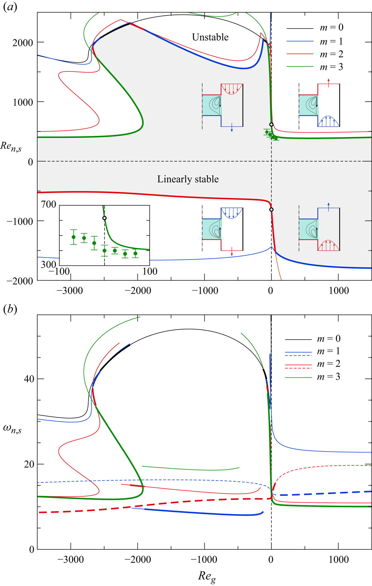
Figure 2. (a) Neutral (thin lines) and critical (thick lines) Reynolds numbers  ${Re}_{n,s}$ as functions of the gas flow Reynolds number
  ${Re}_{g}$. The neutral and critical wavenumbers are coded by colour (legend). The region of linear stability is filled in grey. The insets serve to symbolise the direction and the temperature (hot/cold) of the mean gas flow. The vertical dashed line indicates a vanishing gas flow (closed chamber) and the circles represent the associated critical points. Green dots represent critical Reynolds numbers measured by Ueno et al. (Reference Ueno, Kawazoe and Enomoto2010) for the slightly different aspect ratio
  $\varGamma =0.64$. (b) Corresponding neutral and critical frequencies
  $\omega _s$ (for modes propagating in the negative
  $\varphi$ direction). Full and dashed lines correspond to
  ${Re}_{n,s}>0$ and
  ${Re}_{n,s}<0$, respectively. An enlarged view of (a) and (b) is provided in figure 3 for
  ${Re}>0$ around
  ${Re}_{g}\approx 0$.
For heating from above ( ${Re}>0$) and if the liquid bridge is exposed to a cold, upward gas flow opposing the thermocapillary-driven surface flow (first quadrant in figure 2a), the critical wavenumber is
  $m_c=3$ and
  ${Re}_c$ decreases from
  ${Re}_c({Re}_{g}=0)=616$ when
  ${Re}_{g}$ is increased. Except for a very shallow minimum of
  ${Re}_c$ at
  ${Re}_{g}=450$, the critical Reynolds number
  ${Re}_c({Re}_{g})$ almost saturates near
  ${Re}_c \approx 390$, already for
  ${Re}_{g}\gtrsim 100$. If, on the other hand,
  ${Re}_{g}$ is decreased from zero (hot, downward gas flow parallel to the thermocapillary surface flow, second quadrant in figure 2a), the critical Reynolds number strongly increases up to
  ${Re}_c\approx 2000$ for
  ${Re}_{g}= -60$. This stabilisation was also found experimentally by Ueno et al. (Reference Ueno, Kawazoe and Enomoto2010) for the slightly different aspect ratio
  $\varGamma =0.64$ with the same critical wavenumber
  $m_c=3$ (cf. green dots in figure 2a). For a stronger flow of the hot gas
  $({Re} < -60)$ different modes become critical and the critical curve is made of segments of neutral modes with different azimuthal wavenumbers. This is illustrated in figure 3 by zooming into the region
  $({Re}_{g},{Re}_c) \in [-200,20]\times [1700,2200]$. Most notable is the local minimum of
  ${Re}_c$ at
  ${Re}_{g}=-414$ for wavenumber
  $m=1$ (blue). A similar local minimum of
  ${Re}_c$ for hot co-flow and a mode with
  $m=1$ arises for long liquid bridges with
  $\varGamma =1.8$ of
  ${Pr}=68$ under zero gravity (Stojanovic & Kuhlmann Reference Stojanović and Kuhlmann2020b). The mode with
  $m=1$ (blue) is critical in the range
  ${Re}_{g}\in [-1850,-100]$. The codimension-two points
  $({Re}_{g},{Re}_c)^{m_1,m_2}$ at which two neutral curves for different wavenumbers
  $m_1$ and
  $m_2$ intersect are listed in table 4 (columns labelled ‘static’). Interestingly, the critical Reynolds number for strong gas flow is not a unique function of
  ${Re}_{g}$ in the range
  ${Re}_{g}\in [-2672,-1920]$. In this region the most dangerous mode has a wavenumber
  $m=3$ (green). For even larger downward flow rates
  $({Re}_{g} < -2672)$, the critical Reynolds number saturates near
  ${Re}_c\approx 400$, within the range of
  ${Re}_{g}$ considered.
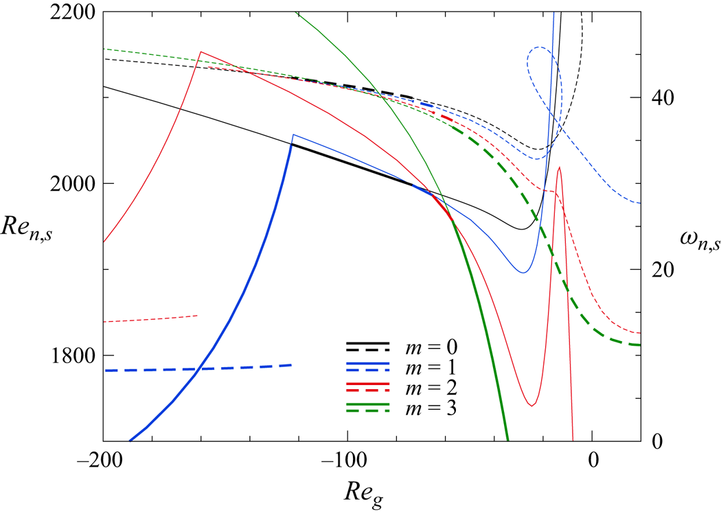
Figure 3. Neutral Reynolds numbers  ${Re}_{n,s}$ (thin solid lines) and neutral frequencies (thin dashed lines) as functions of the gas flow Reynolds number
  ${Re}_{g}\in [-200,20]$ for heating from above (
 ${Re}_{n,s}>0$). Critical Reynolds numbers
  ${Re}_{c,s}$ and frequencies
  $\omega _{n,s}$ as shown as thick lines.
Table 4. Codimension-two points  $({Re}_{g},{Re}_c)^{m_1,m_2}$ for heating from above
  $({Re}>0)$. Data are given for a static as well as for a dynamically deformed free surface of the basic flow.
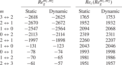
In case of heating from below ( ${Re}_c<0$ in figure 2a) the critical Reynolds number for a closed chamber is
  ${Re}_c({Re}_{g}=0)=-811$ with
  $m_c=2$. Like for heating from above, the critical threshold near
  ${Re}_{g}\approx 0$ is very sensitive with respect to a variation of the gas flow rate. When the liquid bridge is exposed to a cold gas flow from above opposing the thermocapillary flow direction (third quadrant in figure 2a), the basic flow is destabilised and the critical Reynolds number readily saturates near
  ${Re}_c\approx -580$. For a hot gas flow from below (
 ${Re}_{g}>0$, co-flow direction, fourth quadrant in figure 2a), the basic flow is strongly stabilised, the critical wavenumber changes to
  $m_c=1$ at
  ${Re}_{g}=58.5$ and, for
  $1000\lesssim {Re}_{g}\leq 1500$, the critical Reynolds number seems to saturate near
  ${Re}_c\approx -1800$.
For an open shield tube and outflow boundary conditions (2.28) for the basic flow we find slightly different critical Reynolds numbers as  ${Re}_{g}=0$ is approached from above or from below. For heating from above, for instance, we obtain
  ${Re}_c({Re}_{g} \to 0^-)=622$ and
  ${Re}_c({Re}_{g} \to 0^+)=620$. Both these values deviate less than 1 % from the critical Reynolds number
  ${Re}_c({Re}_{g}\equiv 0)=616$ for a closed tube, using rigid boundary conditions
  ${(\boldsymbol{u}_{{g}0}=0)}$ at the outlet. Therefore, and due to the practical relevance of a truly closed ambient gas space, we used rigid boundary conditions only for
  ${Re}_{g}\equiv 0$. Graphically, the minute discontinuity at
  ${Re}_{g}=0$ is not visible with the bare eye in figure 3 (see dashed lines close to
  ${Re}_{g}=0$). Moreover, the discontinuity disappears for
  $\varGamma _{rod}\to \infty$, which is consistent with the critical Reynolds numbers being rather insensitive with respect to increasing
  $\varGamma _{rod}$. In Appendix B it is shown that for
  $|{Re}_{g}| > 90$, the critical Reynolds number varies by less than 2 % when
  $\varGamma _{rod}$ is increased from 0.4 to 8. The results obtained are thus applicable for a wide range of experimental designs with different
  $\varGamma _{rod}$.
4.1.2. Sensitivity of  ${Re}_c$ with respect to the direction of the gas flow

Basic state. In order to understand the strong sensitivity of the critical Reynolds number with respect to the direction and strength of a weak axial gas flow we inspect the basic flows for four cases, each in one of the four quadrants of figure 2(a). For heating from above we consider  $({Re}_{g},{Re})=(\pm 40,616)$, where
  ${Re}={Re}_c({Re}_{g}=0)=616$. For heating from below we similarly select
  $({Re}_{g},{Re})=(\pm 40,-811)$, where
  ${Re}={Re}_c({Re}_{g}=0)=-811$. The basic flows for the four parameter sets are shown in figure 4. For the counterflow configurations in figure 4(b,c) a weak recirculation zone is created in the gas phase next to the free surface, visible by the separation streamline shown. This type of separated flow in the gas phase has been confirmed experimentally by Irikura et al. (Reference Irikura, Arakawa, Ueno and Kawamura2005) and Ueno et al. (Reference Ueno, Kawazoe and Enomoto2010).

Figure 4. Streamlines and temperature fields of four basic states for (a)  $({Re}_{g},{Re})=(-40,616)$ (stable); (b)
  $({Re}_{g},{Re})=(+40,616)$ (unstable); (c)
  $({Re}_{g},{Re})=(-40,-811)$ (unstable); and (d)
  $({Re}_{g},{Re})=(+40,-811)$ (stable). Streamlines are drawn equidistantly. The steps size
  $\Delta \psi$ is pairwise identical in the liquids of (a,b) and in the gases of (a,b). The same applies to (c,d), but with different levels due to the different Reynolds number
  ${Re}$. Note the flow separates from the cold wall in (a,b).
For the present Prandtl number  ${Pr}=28$ the thermal conditions in the gas phase are much more important for the stability than the viscous stresses exerted on the interface by the gas flow. In particular, the flow along the free surface is primarily driven by thermocapillary forces near the hot corner (Kamotani & Ostrach Reference Kamotani and Ostrach1998; Kuhlmann Reference Kuhlmann1999). The cold corner region is of lesser importance, because the strong gradients of the surface temperature near the cold corner are located very close to the rigid wall. Therefore, they cannot contribute significantly to the global flow.
Figure 5(a) shows velocity (blue) and temperature profiles (red) of the basic flow along the free surface for the case of heating from above  $({Re}>0)$. The direction of the gas flow is distinguished by line type. For a hot (cold) gas flow the interface is heated (cooled) for
  ${Re}_{g}=-40$ (
 ${Re}_{g}=40$) as compared with the case of a closed chamber (
 ${Re}_{g}=0$, full line). For a hot downward flow with
  ${Re}_{g}=-40$ (dashed lines), the plateau temperature is increased. This reduces the thermocapillary stresses near the hot corner. As a result, the magnitude of the surface velocity decreases. The cooling of the interface for
  ${Re}_{g}=40$ (dotted lines), on the other hand, reduces the surface temperature in the plateau region and increases the thermocapillary stresses near the hot corner. This gives rise to a larger surface velocity as compared with
  ${Re}_{g}=0$. Viscous stresses from the gas phase would have the opposite effect, but for
  ${Re}_{g} = \pm 40$ they are of minor importance compared with thermocapillary stresses. The stronger flow for
  ${Re}_{g}=40$ as compared with
  ${Re}_{g}=0$ (both at
  ${Re}=616$) is equivalent to a stronger effective thermocapillary driving and can, thus, be identified as the reason for the instability of this flow (shown in figure 4b). Likewise, the weaker thermocapillary driving is responsible for the stability of the flow for
  $({Re}_{g},{Re})=(-40,616)$ (figure 4a).

Figure 5. Tangential velocity  $u_{t0}=\boldsymbol {t}\boldsymbol{\cdot}\boldsymbol {u}_0$ (blue) and temperature distribution
  $\vartheta _0$ (red) of the basic flow along the free surface (parameterised by
  $z$). (a) Heating from above with
  ${Re} = 616$. (b) Heating from below with
  ${Re} = -811$. The gas Reynolds number is distinguished by line type:
  ${Re}_{g}=-40$ (dashed lines),
  ${Re}_{g}=0$ (full lines) and
  ${Re}_{g}=40$ (dotted lines). The insets resolve the velocity peaks near the cold wall.
Apart from the strength of the surface flow, the whole structure of the vortex in the liquid phase and the associated temperature field changes: the radial extent of the stronger vortex (cold upward counter-flow,  ${Re}_{g}=40$, figure 4b) is significantly larger than that of the weaker vortex (hot downward co-flow,
  ${Re}_{g}=-40$, figure 4a). This effect results from the interplay between buoyancy and inertia forces. Heating the liquid bridge from above, hot liquid is transported downward along the free surface and returns upward in the bulk. Since the upward motion in the bulk is assisted by buoyancy forces, the radial extension of the vortex is reduced compared with the case of zero gravity. This effect is most pronounced when the thermocapillary-driven vortex flow is weak
  ${Re}_{g}=-40$ (figure 4a). For the stronger basic flow at
  ${Re}_{g}=40$, inertia prevents a premature buoyant rise of the liquid in the bulk and the vortex has a larger extent in the radial direction (figure 4b). Associated with this change of the vortex structure, the region of large (mainly radial) internal temperature gradients is displaced radially inward for
  ${Re}_{g}=40$ (figure 4b) and radially outward for
  ${Re}_{g}=-40$ (figure 4a). This structural change has implications for the respective critical mode and the stability boundary, because a hydrothermal wave draws its energy primarily from the internal basic state temperature gradients (Smith & Davis Reference Smith and Davis1983a; Wanschura et al. Reference Wanschura, Shevtsova, Kuhlmann and Rath1995).
For heating from below (figures 4c,d and 5b) similar arguments hold. For example, for  ${Re}_{g} = 40 > 0$ (figure 4d), the free surface is heated (dotted red line in figure 5b), which reduces the thermocapillary driving near the hot wall. As a result, the flow for
  ${Re}_{g}=40$ is much weaker and more stable than that for
  ${Re}_{g}=0$ and
  ${Re}_{g}=-40$ (both at
  ${Re}=-811$). While the structure of the basic vortices is similar for both directions of the gas flow (
 ${Re}_{g} = \pm 40$, figure 4c,d) and heating from below, they differ markedly from those for heating from above: for heating from below, buoyancy is assisting the upward free surface flow but tends to prevent the hot return flow from descending. This leads to a much larger radial width of the vortices (figure 4a,b) associated with a further inward displacement of the internal temperature gradients than for heating from above (figure 4a,b).
In summary, for a weak gas flow, the basic flow is stronger in the counter-flow configuration, due to the heat transfer between liquid and gas. Furthermore, buoyancy forces cause the flow structures to be located closer to the free surface for heating from above, while they are displaced radially inward for heating from below.
Critical modes. The instability for  ${Re}_{g}=0$ is due to hydrothermal waves (Smith & Davis Reference Smith and Davis1983a; Wanschura et al. Reference Wanschura, Shevtsova, Kuhlmann and Rath1995). They are generated in the liquid phase and depend on the structure of the flow in the liquid. Taking into account the gas phase, Stojanovic et al. (Reference Stojanović, Romanò and Kuhlmann2022) have shown that the temperature amplitude of the hydrothermal wave is very weak in the gas phase. Therefore, the gas phase only plays an indirect role for the instability process by affecting the basic velocity and temperature fields in the liquid phase. Since the hydrothermal waves depend on the particular basic flow structure, we consider representative critical modes with
  $\omega _c > 0$, corresponding to waves propagating in the negative
  $\varphi$ direction.
Let us compare the critical mode for heating from above and  ${Re}_c({Re}_{g}=-40) = 1786$ (hot downward gas co-flow) with that for
  ${Re}_c({Re}_{g} = 40)=431$ (cold upward gas counter-flow). Both modes have the wavenumber
  $m_c=3$. From figure 6(a,b) the location of the regions of high basic state temperature gradients is qualitatively similar as in figure 4(a,b) for
  ${Re}=616$. However, for cold upward gas counter-flow (figure 6b,
  $({Re}_{g},{Re}_c)=(40,431)$), the temperature gradients of the basic flow from which the hydrothermal wave draws its energy are located more distant from the free surface than for hot downward gas co-flow (figure 6a,
 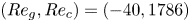 $({Re}_{g},{Re}_c)=(-40,1786)$). This provides more space for the evolution of the perturbation vortices which feed the perturbation temperature extrema by advecting basic state temperature (Wanschura et al. Reference Wanschura, Shevtsova, Kuhlmann and Rath1995). Figure 6(a–d) shows that the perturbation vortices at criticality are well developed for
  ${Re}_{g}=40$, whereas they are more confined to the free surface region for
  ${Re}_{g}=-40$. Therefore, the critical mode for
 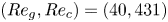 $({Re}_{g},{Re}_c)=(40,431)$ can draw its energy from a larger region of high basic state temperature gradients than the critical mode for
  $({Re}_{g},{Re}_c)=(-40,1786)$ and the perturbation temperature field for
  ${Re}_{g}=40$ is more compact, presumably suffering less thermal dissipation than the less compact one for
  ${Re}_{g}=-40$. While the structures of the two critical modes differ in the bulk, their footprints on the free surface are very similar (figure 6e, f).

Figure 6. Critical velocity (black arrows) and temperature fields (colour) for heating from above and hot co-flow  $({Re}_{g},{Re}_c)=(-40,1786)$ (a,c,e) and cold counter-flow
  $({Re}_{g},{Re}_c)=(40,431)$ (b,d, f). The colour bars are normalised with respect to the maximum temperature perturbation for each subfigure. The critical wavenumber is
  $m_c=3$. (a,b) Vertical
  $(r,z)$ planes in which the local thermal production (not shown) takes its maximum (white cross) in the bulk. Lines in (a,b) indicate equidistant isotherms of the basic state. (c,d) Horizontal cross-sections in the planes
  $z=-0.36$ (c) and
  $z=0.03$ (d) in which the respective total local thermal production
  $-\vartheta ' \boldsymbol {u}' \boldsymbol{\cdot} \boldsymbol {\nabla } \vartheta _0$ (isolines) takes its maximum (white crosses) in the bulk. (e, f) Radial projections of the free surface velocity and temperature. The grey arrows in (c,d,e) indicate the direction of propagation of the critical mode. The dashed lines represent the location of the vertical and horizontal cut planes.
For heating from below the critical modes for 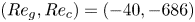 $({Re}_{g},{Re}_c)=(-40,-686)$ and
  $({Re}_{g},{Re}_c)=(40,-1348)$ are shown in figures 7(a,c,e) and 7(b,d, f), respectively. In contrast to heating from above, both critical modes have wavenumber
  $m_c=2$ and they may appear very similar for
  ${Re}_{g}=\pm 40$ (figure 4c,d). But the stronger basic vortex at constant
  ${Re}$ for
  ${Re}_{g}=-40$ as compared with
  ${Re}_{g}=40$ explains why the former is more unstable than the latter. Another contributing factor, visible from figure 4(a–d), is the radial temperature gradients of the basic flow arise closer to the axis for
  ${Re}_{g}=40$ as compared with
  ${Re}_{g}=-40$. Therefore, the coupling between internal temperature extrema and the surface temperature fluctuations driving the perturbation velocity field is weaker for
  ${Re}_{g}=40$.

Figure 7. Critical modes for heating from below and for  $({Re}_{g},{Re}_c)=(-40,-686)$ (a,c,e) and for
  $({Re}_{g},{Re}_c)=(40,-1348)$ (b,d, f). Lines, arrows and colours as in figure 6. The horizontal cuts are located at
  $z=0.04$ (a,e) and
  $z=0.1$ (b, f). The critical wavenumber is
  $m_c=2$.
The thermal energy budgets for the four critical modes considered are presented in figure 8. From figure 8(a) all critical modes are hydrothermal waves for which the perturbation energy is mainly created by radial advection of basic state temperature, represented by the total normalised production term  $J_1:= -{Re} {\mathcal {D}}_{th}^{-1}\int _{V_i} j_1 \,\mathrm{d} V = -{Re} {\mathcal {D}}_{th}^{-1}\int _{V_i} \vartheta ' u' \partial _r \vartheta _0\,\mathrm{d} V$. The thermal production by axial advection
  $J_2:= -{Re} {\mathcal {D}}_{th}^{-1}\int _{V_i} j_2 \mathrm{d} V = -{Re} {\mathcal {D}}_{th}^{-1}\int _{V_i} \vartheta ' w' \partial _z \vartheta _0\,\mathrm{d} V$ plays a minor role. For heating from above (solid colours) the critical mode for
  ${Re}_{g}=-40$, which is confined to the very vicinity of the free surface, has the smallest production
  $J_1 = 0.778$ (full red bar) and deviates the most from the reference value of
  $J_1$ for
  ${Re}_{g}=0$ (full orange bar). It is also seen that the heat loss of the liquid phase through the free surface, i.e. the thermal coupling, is generally vanishingly small compared to the thermal production due to advection
  $(J_1, J_2)$ in the liquid (figure 8a). This small heat loss of the perturbation flow in the liquid
  $H_{fs}:=2{\rm \pi} {\mathcal {D}}_{th}^{-1}{Pr}^{-1}\int _{-0.5}^{0.5}h(\partial _r\hat {\vartheta }^2-\partial _z h_0\partial _z\hat {\vartheta }^2)\,\mathrm{d} z$ appears as a heat gain
 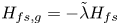 $H_{fs,g}=-\tilde {\lambda }H_{fs}$ of the perturbation flow in the gas phase. There it is the main source of thermal energy. But this gain is almost completely balanced by the thermal dissipation in the gas phase
  $D_{{th},g}$. This proves quantitatively the gas phase does not play an active role in the instability mechanism. As a side, the relative thermal production rates
  $\varPi _\rho <0.1\,\%$ and
  $\varPi _{\rho,{g}} < 1\,\%$ associated with the density variations in the liquid and in the gas, respectively, are negligible.
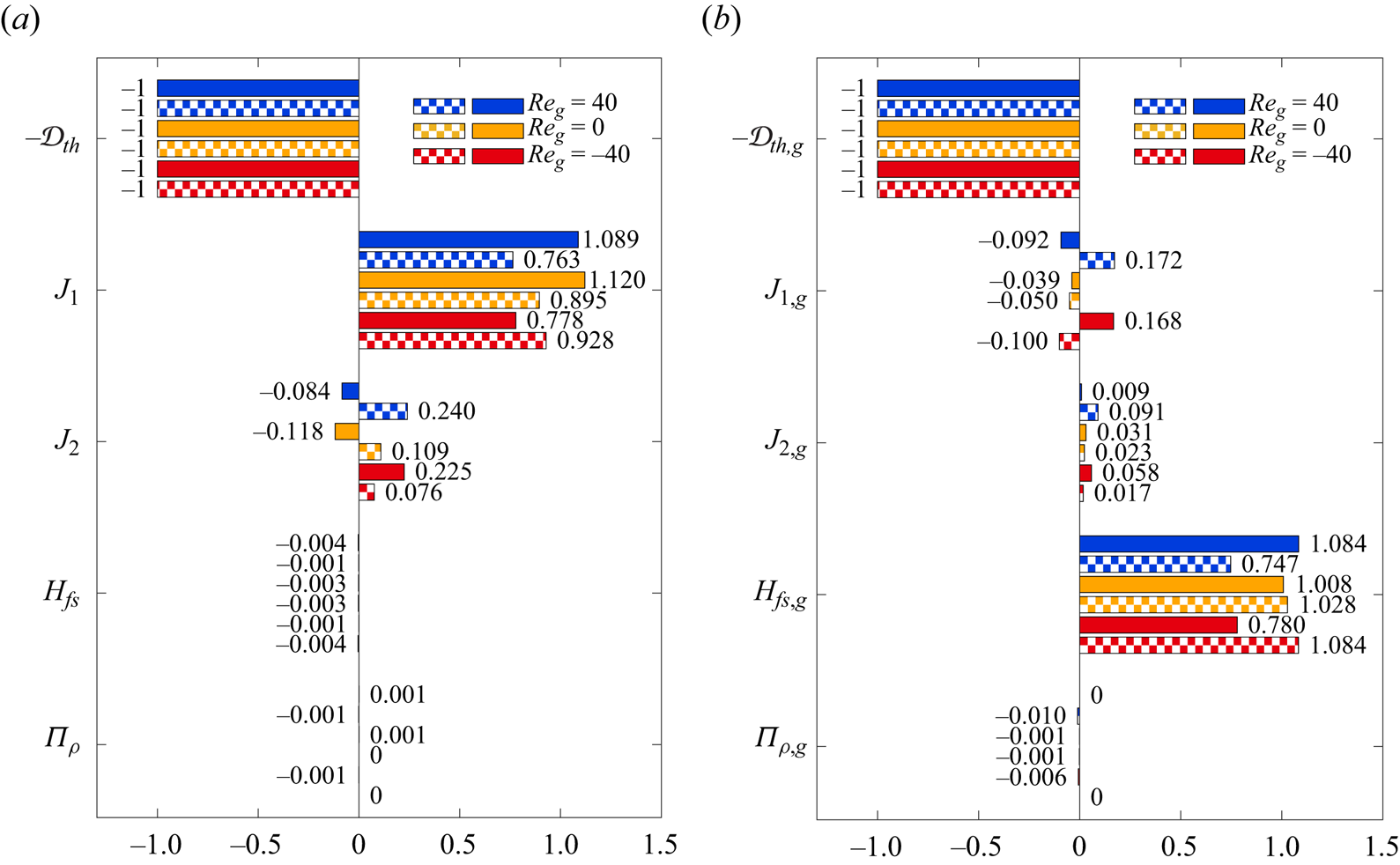
Figure 8. Thermal energy budgets of the critical modes for  ${Re}_{g} \in \{-40;0;40\}$. (a) Liquid phase; (b) gas phase. Full bars: heating from above with
  ${Re}_c \in \{1786;616; 431\}$ and
  $m_c=3$. Checkered bars: heating from below with
  ${Re}_c \in \{-686; -811; -1348\}$ and
  $m_c=2$
In conclusion, we find the sensitivity of the critical Reynolds number with respect to a weak axial gas flow is mainly related to the changed strength of the basic flow, caused by the heating or cooling of the free surface by the gas flow. The strength of the basic flow affects the strength of the basic state temperature gradients and, thus, the stability boundary. The critical wavenumbers differ for heating from above  $(m_c=3)$ and from below
  $(m_c=2)$. But the spatial structures of the critical modes do not change very much, except for heating from above with
  ${Re}_{g}<0$ in which the weaker vortex is also radially more confined to the interface as a result of buoyancy.
4.1.3. Critical modes for large gas flow rates: heating from above
Three-dimensional views of the critical modes for heating from above are shown in figure 9(a–e) by isosurfaces of the perturbation temperature  $\vartheta '$ for
  ${Re_{g}=(-3000, -1000, -40, 40, 1000)}$, covering the full range of gas flow Reynolds numbers. All waves propagate in clockwise, i.e. in the negative
  $\varphi$ direction. Since the dynamic Bond number is constant with
  ${Bd}=0.41$, buoyancy forces are proportional to the thermocapillary forces. The critical wavenumber of the modes shown is
  $m_c=3$, except for
  ${Re}_{g} = -1000$ for which
  $m_c=1$. Throughout, the temperature perturbations exhibit the typical behaviour of a hydrothermal wave. Merely, for
  ${Re}_{g}=-1000$ (figure 9b) and
  ${Re}_{g}=-40$ (figure 9c) where the critical Reynolds numbers are relatively large with
  ${Re}_c \approx 1750$, the critical modes differ. In these cases buoyancy forces are strong as well, while the surface flow is weakened due to the hot gas co-flow
  $({Re}_{g} < 0)$. In these cases the Rayleigh number
  ${Ra} = 11.48 \times {Re}$ can reach values of the order of
  $O(10^4)$ (stabilising thermal stratification). Thus, buoyancy shapes the basic vortex close to the free surface to have a much smaller radial extent (for
  ${Re}_{g}<0$) than for smaller Reynolds (and Rayleigh) numbers and the temperature extrema of the hydrothermal wave for
  ${Re}=-1000$ and
  $-40$ arise much closer to the free surface (see e.g. figure 6a,c). These perturbation modes also have a more spiral behaviour such that the perturbation temperature field exhibits a more complex structure in a plane
  $\varphi =\textrm {const.}$ with temperature minima and maxima, visible in figure 6(a).
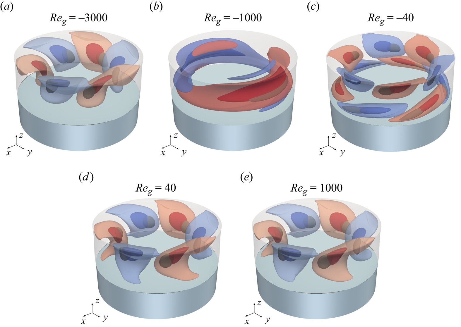
Figure 9. Isosurfaces of the critical perturbation temperature  $\vartheta '$ in the liquid for heating from above:(a)
  ${Re}_c=404$; (b)
  ${Re}_c=1733$; (c)
  ${Re}_c=1786$; (d)
  ${Re}_c=431$; (e)
  ${Re}_c=389$. The isosurface values are
  $\pm 0.25 \times \max | \vartheta ' |$ (light colours) and
  $\pm 0.75 \times \max | \vartheta ' |$ (dark colours). A single isosurface of the total local thermal production rate at
  $j_1+j_2 = \vartheta ' \boldsymbol {u}' \boldsymbol{\cdot} \boldsymbol {\nabla } \vartheta _0= 0.7\times \max |\vartheta ' \boldsymbol {u}' \boldsymbol{\cdot} \boldsymbol {\nabla } \vartheta _0|$ is shown in grey.
For a discussion of the saturation of the critical Reynolds numbers seen in figure 2(a), we note that the viscous stress from the gas phase has very little influence on the basic flow for the range of gas Reynolds numbers considered. Estimating the magnitude of the thermocapillary stress by  $\gamma \Delta T/d$ and the viscous stress due to the gas flow by
  $\mu _g \bar w_{g}/(r_{o} - r_{i})$, the order of magnitude of the ratio of the viscous gas stress to the thermocapillary stress is
  $\varGamma \tilde \mu ({Re}_{g}/3{Re})$. For
  ${Re}_{g}=3000$ and
  ${Re}=500$ this amounts to about 1 %. Therefore, within the range of
  ${Re}_{g}$, the effect of the gas flow on the basic state is essentially thermal.
For heating from above and cold counter-flow  $({Re}_{g} > 0)$ the critical Reynolds number saturates at relatively small gas flow rates of
  ${Re}_{g} \approx 100$ at a value of
  ${Re}_c\approx 390$. For this Reynolds number the basic vortex flow and temperature field in the liquid are almost independent of the gas Reynolds number in the range
  ${Re}_{g}\in [100,500]$. This can be explained by two opposing thermal effects of the gas flow on the strength of the vortex which nearly balance each other at
  ${Re}=390$. To understand these effects, radial profiles of the vertical velocity
  $w(r)$ at midplane
  $z=0$ are shown in figure 10 for several thermocapillary Reynolds numbers (colour coded) and
  ${Re}_{g}=40$ (dashed lines) and
  $1000$ (full lines).
Figure 10. Dimensional axial velocity component  $w(r,z=0)$ at midplane for different thermocapillary Reynolds numbers (colours) and for gas flow Reynolds numbers
  ${Re}_{g}=40$ (dashed lines) and
  ${Re}_{g}=1000$ (full lines). The inset serves to show the scale of the gas flow relative to the liquid flow for
  ${Re}=1000$. The location of the interface is at
  $h_0(z=0)=2.5$ mm.
For a vanishing thermocapillary Reynolds number  ${Re}=0$, the flow in the liquid is only driven by the gas (orange lines) and the interface moves in the positive
  $z$ direction with
  $w(r=h_0(0))>0$. As
  ${Re}$ is increased the surface flow becomes readily dominated by thermocapillary forces and for
  ${Re}=100$ the direction of the surface velocity is downward with
  $w(r=h_0(0))<0$ (red lines). For
  ${Re}=100$ and weak gas counter-flow (
 ${Re}_{g}=40$, dashed red line) a separation bubble of considerable size exists in the gas phase next to the free surface (see e.g. figure 4b), visible in figure 10 by the downward gas flow between the free surface (
 $r\approx 2.50$ mm) and the zero of
  $w_{g0}(r)$ in the gas phase at
  $r\approx 2.53$ mm. For the stronger gas counterflow (
 ${Re}_{g}=1000$, full red line) the region in which
  $w_{g0}<0$ in the gas phase adjacent to the free surface has become very thin due to the higher shear stress in the gas phase. The zero of
  $w_{g0}$ has moved very close to the free surface (almost invisible on the scale shown) and
  $w_{g0}$ (full red line) increases nearly vertically for
  $r > h_0(0)$. As expected, the stronger gas flow has a retarding effect on the downward surface flow due to the increased viscous stresses from the gas on the interface. Associated with the reduced surface velocity is a weaker vortex in the liquid. As the thermocapillary Reynolds number is increased to
  ${Re}\approx 400$ (blue lines), which roughly coincides with the saturation of
  ${Re}_c({Re}_{g})$, the retardation of the surface velocity diminishes. For
  ${Re}\gtrsim 400$ the gas flow has an augmenting effect on the magnitude of the interfacial velocity, despite of the retarding action of the viscous shear stresses from the gas side. As a result, the magnitude of the surface velocity for
  ${Re}=1000$ is larger for
  ${Re}_{g}=1000$ (full green line) than for
  ${Re}_{g}=40$ (dashed green line). The reason for the augmenting action of the counterflow is related to the characteristic surface temperature profile when the thermocapillary Reynolds number is large and the flow is mainly driven near the hot corner (the argument was used in explaining the velocity profiles in figure 5): the gas has a cooling effect such that the plateau temperature for large-thermocapillary-Reynolds-number flows is decreased. Along with a decrease of the plateau temperature the thermocapillary driving force near the hot wall increases and reinforces the thermocapillary flow, overcompensating the viscous retardation effect. For
  ${Re}\gtrsim 400$ the increase of the surface velocity at midplane by the cooling effect is larger than the decrease of the surface velocity due to viscous stresses from the gas side which, on the other hand, dominates for
  ${Re}\lesssim 400$.
The Reynolds number  ${Re}\approx 400$ at which both effects on the surface velocity
  $w(r=h_0(0),0)$ balance seems to be almost independent of
  ${Re}_{g}\in [100,500]$. Therefore, the whole basic flow for
  ${Re}\approx 400$ is almost independent of
  ${Re}_{g}$ in this range, and a critical Reynolds number
  ${Re}_c\approx 400$ will also be independent within
  ${Re}_{g}\in [100,500]$. In fact, the radial temperature gradients for
  ${Re}=400$ from which the hydrothermal-wave instability draws its energy are almost independent
  ${Re}_{g}\in [100,500]$. This is demonstrated in figure 11 which shows basic temperature profiles
  $\vartheta _0(r,z=0)$ at midplane for
  ${Re}=400$ (
 $\approx$ saturation level of
  ${Re}_c$) and different gas Reynolds numbers
  ${Re}_{g}=20$, 50, 100, 200 and 500. In the region
  $r\le 1.1$ of largest slopes, the temperature profiles are almost identical, regardless of the temperature gradients in the gas phase. This indicates the perturbation mode finds the same basic-flow conditions for the major energy production term
  $J_1$ which builds on
  $\partial _r\vartheta _0$ in the liquid phase, independent of
  ${Re}_{g}$. On the other hand, the slope for
  ${Re}_{g}=500$ and
  ${Re}=200$ (black dashed line) is smaller, while the one for
  ${Re}_{g}=500$ and
  ${Re}=600$ (black dash-dotted) is larger. These flow states are stable and unstable, respectively. From figure 11 one can also identify the continuous decrease of the surface temperature as
  ${Re}_{g}$ is increased.
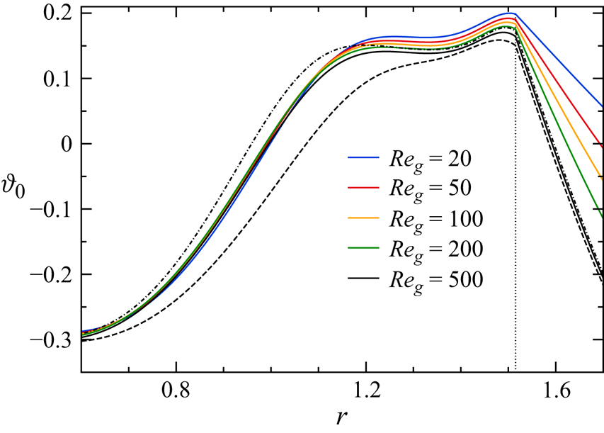
Figure 11. Radial basic temperature profiles  $\vartheta _0(r,z=0)$ for
  ${Re}=400$ and different gas Reynolds numbers
  ${Re}_{g}=20$, 50, 100, 200 and 500 (full lines colour coded, see legend). In addition, the temperature profiles are shown for
  ${Re}_{g}=500$ and
  ${Re}=200$ (black dashed) and
  ${Re}=600$ (black dash-dotted). The vertical dotted line marks the free surface.
The major integral (global) energy production terms  $J_1$ and
  $J_2$ for the liquid phase are displayed in figure 12 as functions of
  ${Re}_{g}$. For the major critical modes with
  $m_c=1$ (blue),
  $m_c=2$ (red) and
  $m_c=3$ (green), the thermal energy is mainly produced by radial advection of basic state temperature
  $J_1$ (full lines). The axial advection (dashed lines) is almost negligible or even acts stabilising. This applies to both gas flow directions. Hence, the instability mechanism as such is not much affected by the direction of the gas flow, i.e. by the heating or cooling of the liquid through the gas in the basic flow. The peak values of the total local energy production
  $j_1 + j_2$ are located inside the grey isosurfaces shown in figure 9. Typically, the production maxima are azimuthally displaced from the temperature extrema with the displacement direction determining the direction of propagation of the wave.

Figure 12. (a) Normalised global energy production rates  $J_1$ (full lines) and
  $J_2$ (dashed lines) of the critical (and neutral) modes in the liquid phase for heating from above shown as functions of
  ${Re}_{g}$. The colour indicates the wavenumber. The vertical dotted lines indicate the codimension-two points listed in table 4. (b) Enlarged view of the grey rectangle shown in (a).
For all  ${Re}_{g}$ considered,
  $|\varPi _\rho |<0.002$ and
  $-0.007< H_{fs}<0$ in the liquid phase. The greatest impact of the density variation on the thermal energy budget is observed in the gas phase and for heating from above with
  $\varPi _{\rho,{g}}=-0.021$ for
  $m_c=2$,
  ${Re}_{g}=-2114$,
  ${Re}_c=2311$. This conditions corresponds to
  $\Delta T=70\,$K and
  $\varepsilon =0.087$. For heating from below, the maximum impact of
  $\varPi _{\rho,{g}}$ on the thermal energy is found to be even smaller (not shown).
4.1.4. Critical modes for large gas flow rates: heating from below
Figure 13 shows temperature isosurfaces of the critical modes for heating from below and for the same gas flow Reynolds numbers as in figure 9. Now the dominant critical wavenumber is  $m_c=2$ and most critical modes have the expected structure with strong internal temperature extrema in the shear layer of the return flow of the basic vortex. Only for stronger hot co-flow from below with
  ${Re}=1000$ the wavenumber changes to
  $m_c=1$ and the critical mode is very different from the others with a pronounced spiral character and temperature extrema very close to the axis. In this case the basic flow is affected by the gas flow in an opposite manner than for hot co-flow when heating from above: instead of a small radial extent of the basic vortex for heating from above, the basic vortex is radially extended for heating from below, because the hot fluid transported upward along the free surface has the tendency to stay near in the upper half of the liquid bridge such that the return flow arises closer to the axis. This facilitates an
  $m_c=1$ mode with a flow across the axis to extract thermal energy from the basic temperature field. The trend that the temperature extrema move closer to the axis (following the location of high basic temperature gradients) is already visible for
  ${Re}_{g}=40$ in figure 13(e).

Figure 13. Isosurfaces of the critical perturbation temperature  $\vartheta '$ in the liquid for heating from below:(a)
  ${Re}_c=-515$; (b)
  ${Re}_c=-615$; (c)
  ${Re}_c=-686$; (d)
  ${Re}_c=-1348$; (e)
  ${Re}_c=-1778$. Colours and isosurface values as in figure 9.
The critical modes for  ${Re}_{g}=40$ and
  ${Re}_{g}=1000$ are displayed in figure 14. It can be seen that the critical velocity field for
  ${Re}_{g}=1000$ is oblique to the basis state isotherms near the point of maximum thermal energy production (white cross). Therefore, the critical mode can also gain energy from the vertical temperature gradients such that
  $J_2$ has a bigger share in the thermal energy budget, which is shown in figure 15. Remarkable is the spiral character of the isosurfaces of the perturbation temperature near the upper cold wall in figure 13(e). These spiral arms show in figure 14(b) as a sequence of hot and cold spots in the upper part of the region with high temperature gradients. A similar hydrothermal wave with an even more pronounced spiral character arises in liquid bridges with the still higher Prandtl number
  ${Pr}=68$ (Stojanovic & Kuhlmann Reference Stojanović and Kuhlmann2020a).

Figure 14. Critical modes for heating from below and hot co-flow with  ${Re}_{g}=40$ (a) and
  ${Re}_{g}=1000$(b) in planes
  $\varphi =\textrm {const.}$ in which the local thermal energy production has its maximum (white cross). The perturbation velocity fields (arrows) and the perturbation temperatures (colour) are shown. Isolines of the basic temperature field are drawn in black.
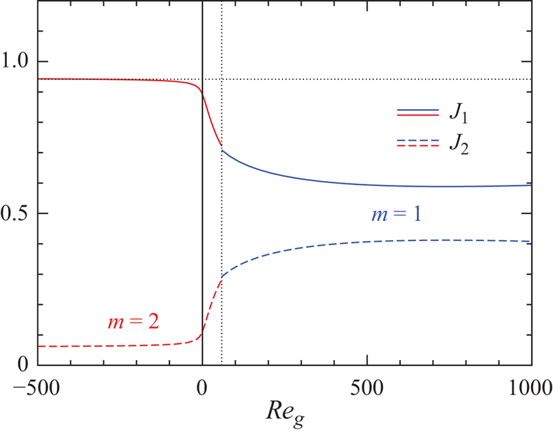
Figure 15. Normalised global energy production rates  $J_1$ (full lines) and
  $J_2$ (dashed lines) of the critical mode in the liquid phase for heating from below shown as functions of
  ${Re}_{g}$. The colour indicates the wavenumber. The vertical dotted line marks the codimension-two point at
  ${Re}_{g}=58.5$. The horizontal dotted line represents
  $J_1({Re}_{g}=-3000)$.
4.2. Dynamic surface shape
In this section we first discuss the causes for and the properties of the dynamic surface shape of the liquid bridge in the basic state. Thereafter, the influence of the dynamic deformability of the interface on the linear stability is discussed.
4.2.1. Static surface shape and dynamic deformation due to the gas flow alone
Static shapes  $h_{0,s}$ of an isothermal liquid bridge, i.e. solutions of (2.23), are shown in figure 16(a) for different filling factors
  $\mathcal {V}$ (colour) and gravity levels (line type) in the absence of any flow. When an axial flow is imposed in the gas phase, with the liquid bridge still being isothermal (
 ${Re}=0$), the dynamic pressure and the normal stresses along the interface modify the static shape. The dynamic deformation
  $\Delta h_0$ of the static shape under zero gravity (
 $0g$) due to a vertically upward gas flow with
  ${Re}_{g}=825$ is shown in figure 16(b) for an underfilling (
 ${\mathcal {V}}\leq 1$) and in figure 16(c) for an overfilling (
 ${\mathcal {V}}> 1$) of the liquid bridge. It can be seen that a constant gas flow rate induces a dynamic deformation which is more than 10 times larger in case of an overfilling as compared with an underfilling. Nevertheless, for this gas flow rate and volume ratios up to
  ${\mathcal {V}}=1$ (full blue line figure 16a) the dynamic deformation
  $\Delta h_0$ is at least three orders of magnitude smaller than the axial variation
  $h_{0,s}(z,1g)-h_{0,s}(z,0g)$ of the hydrostatic shape due to gravity. A gas flow with
  ${Re}_{g}=825$ thus hardly perturbs the interface. For an upright cylindrical liquid bridge (
 ${\mathcal {V}}=1$ and zero gravity, blue dashed line in figure 16a) the shape perturbation
  $\Delta h_0$ (dynamic deformation) is caused by the streamwise pressure drop in the gas flow and leads to a constriction of the bridge in the upstream half and a bulging in the downstream half. The same holds true under gravity conditions. Due to the hydrostatic surface deformation for normal gravity (
 $1g$), the isobars in the gas phase shown in figure 17(a) are more distorted than for zero gravity (
 $0g$). As the volume ratio deviates from
  ${\mathcal {V}}=1$, the contact angles change and the pressure in the gas in the immediate vicinity of the liquid bridge can be strongly affected (figure 17). Typically, a local minimum and a local maximum of the pressure arise. For a large volume (
 ${\mathcal {V}}>1$) with contact angles
  $\alpha > {\rm \pi}/2$ on the liquid side, these pressure extrema lead to qualitatively the same dynamic deformation as expected from the pressure drop in the gas far from the liquid bridge: bulging in the downstream half of the liquid bridge and necking in the upstream half (figure 16c). For small volume ratios (
 ${\mathcal {V}} < 1$) with contact angles
  $\alpha < {\rm \pi}/2$ on the liquid side, the locations of the maximum and minimum pressures in the gas are approximately exchanged and the resulting dynamic deformation
  $\Delta h_0$ exhibits the opposite behaviour: the interface is bulging upstream and constricting downstream (figure 16b). The gravity level does not play an important role for the dynamic deformation, but moderately changes the hydrostatic shape of the bridge.

Figure 16. (a) Hydrostatic shape  $h_{0,s}-1/\varGamma$ of a liquid bridge for the present geometry, different liquid volumes
  $\mathcal {V}$ (colour), zero gravity (
 $0g$, dashed lines) and normal gravity (
 $1g$, full lines). (b,c) Dynamic surface deformation
  $\Delta h_0$ of the static shape in zero gravity due to a gas flow in positive
  $z$ direction with
  ${Re}_{g}=825$
  $({Re}=0)$: (b)
  ${\mathcal {V}}\leq 1$; (c)
  ${\mathcal {V}}>1$. Colours and line types as in (a).

Figure 17. Isobars in the gas phase for  ${Re}=0$ and
  ${Re}_{g}=850$: (a)
  ${\mathcal {V}}=1$ and
  $1g$; (b)
  ${\mathcal {V}}=1.2$ and
  $0g$;(c)
  ${\mathcal {V}}=0.85$ and
  $0g$.
$0g$.
For contact angles  $\alpha <{\rm \pi} /2$ on the liquid side (contact angles
  $\alpha _{g}> {\rm \pi}$ on the gas side) the pressure distribution in the gas is strongly affected by the flow singularities which arise due to the sharp corners. The singularity of the pressure along the inner boundary of the gas space is clearly seen in figure 18. While a detailed analysis would have to include also the liquid phase, we note that the pressure distribution does not change much if the liquid phase is artificially replaced by an indeformable solid with the same shape as the hydrostatic shape (not shown). The reason is the viscosity of the liquid
 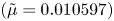 $(\tilde \mu =0.010597)$ is almost 100 times higher than that of the gas. This observation suggests a comparison with the local flow over a corner with opening angle
  $\alpha _{g}> {\rm \pi}$ made by two plane rigid walls. The pressure which results from the Stokes flow asymptotics close to the corner (Moffatt Reference Moffatt1964) diverges and makes a jump when the corner is passed. For the present liquid bridge, we find qualitatively the same behaviour for
  $\alpha _{g}> {\rm \pi}$. The signs of the pressure divergence near the contact lines obviously determine the pressure gradient in the gas and along the interface leading to the pressure extrema shown in figure 17. The pressure variation in the gas flow due to the expansion of the cross-section of the gas flow contributes as well.
Figure 18. Profiles of the pressure  $p_{g}$ along the free surface and the solid rods for a dynamically deformable liquid bridge. The parameters are:
  $0g$,
$0g$,  ${Re}=0$,
  ${Re}_{g}=825$ and volume ratios
  $V$ as indicated.
For large volume ratios  ${\mathcal {V}}>1$ with
  $\alpha _{g} < {\rm \pi}$, the corner flow analysis of Moffatt (Reference Moffatt1964) does not yield corner singularities. In fact, the flow over the contact lines for
  $V>1$ is smooth (figure 18), except for a small indentation in the pressure profile for
  ${\mathcal {V}}=1.2$ at the upper corner. Therefore, the pressure distribution is mainly due to the gas flow deceleration near the upstream half of the liquid bridge and the acceleration near the downstream half. While these considerations can explain the gross features of the pressure distribution and, thus, the qualitative shape of the dynamic deformation
  $\Delta h_0$, the details are also affected by the liquid flow (driven by the gas flow) and the pressure singularities which exist on the liquid side as the contact lines are approached.
An overview of the dynamic deformation  $\Delta h_0$ due to the isothermal gas flow over a liquid bridge with
  ${\mathcal {V}}=1$ in the absence of the thermocapillary effect
  $({Re}=0)$ and for normal gravity condition (
 $1g$) is shown in figure 19. For downward gas flow
  $({Re}_{g}<0)$ parallel to the acceleration of gravity the dynamic deformation leads to a very slight necking tendency of the liquid bridge for
  $z\gtrsim 0$ and slight bulging tendency for
  $z\lesssim 0$, since the pressure gradient in the gas phase along the interface (not shown) has the same sign as the pressure difference between the inlet and the outlet. Upon a reversal of the gas flow direction, the slight necking tendency arises for
  $z\lesssim 0$ and the bulging for
  $z\gtrsim 0$. The black lines in figure 19 indicate the locus
  $z_{max}$ of the maximum of the dynamic deformation
  $\Delta h_0$ and its projection to the
  $(z,{Re}_{g})$ plane. The line is interrupted near
  ${Re}_{g}=0$, where the maximum dynamic deformation drops below
  $\Delta h_0(z) < 5 \times 10^{-6}$, which marks the precision by which the dynamic deformation can be computed by the present numerical approach.

Figure 19. Dynamic surface deformation  $\Delta h_0$ as function of
  $z$ and
  ${Re}_{g}$ for
  ${\mathcal {V}}=1$,
  ${Re}=0$ and
  $1g$. The grey contour lines indicate surface deformations for constant
  ${Re}_{g} \in [-3500; 1500]$ incremented by
  $\Delta {Re}_{g}=500$. The black lines show the loci of maximum of
  $\Delta h_0$ and its projection to the
  $(z,{Re}_{g})$ plane.
Even though the dynamic deformation is insignificant on the scale of the hydrostatic deformation in the gravity field, the dynamic deformation for  ${\mathcal {V}}=1$ and
  $1g$ slightly amplifies the static deformation for
  ${Re}_{g}<0$ such that
  $\max h_{0,d} > \max h_{0,s}$ and
  $\min h_{0,d} < \min h_{0,s}$. For
  ${Re}_{g} > 0$ the reverse holds true (see also figure 16).
4.2.2. Dynamic surface deformation due to the thermocapillary flow alone
The dynamic surface shape  $h_{0,d}$ strongly depends on both
  ${Re}$ and
  ${Pr}$; examples are given in figure 30 in Appendix B. For the present liquid with
  ${Pr}=28$,
  ${Re}\ne 0$, zero gravity (
 $0g$),
  ${\mathcal {V}}=1$ and neglect of the gas phase (single phase flow) the dynamic shape
  $h_{0,d} = h_{0,s} + \Delta h_0$ is always S-shaped, i.e. the dynamic deformation
  $\Delta h_0$ is negative (positive) close to the hot (cold) corner with the extrema of
  $h_{0,d}$ depending on the magnitude of the Reynolds number
  ${Re}$ (not shown).
Here we investigate the influence of the thermocapillary flow alone on the dynamic surface deformation  $\Delta h_0$ under normal gravity (
 $1g$) and in the presence of the gas phase (two-phase flow), but for
  ${Re}_{g}=0$, i.e. for a closed gas container. The dynamic surface deformation is shown in figure 20 for heating from above (
 ${Re}>0$, figure 20a) and for heating from below (
 ${Re}<0$, figure 20b). The dynamic deformation amplifies (reduces) the static deformation for heating from above (below). For heating from above (
 ${Re}>0$, figure 20a), the dynamic deformation has a sinusoidal shape and its strength, measured by its maximum value, depends approximately linearly on
  ${Re}$. The maximum of
  $\Delta h_0$ arises near the lower cold wall. For heating from below (
 ${Re}<0$, figure 20b) the maximum of
  $\Delta h_0$ also arises near the cold wall, which is now the upper wall. But the extrema of
  $\Delta h_0$ arise much closer to the wall such that the dynamic deformation for large absolute values of
  ${Re}<0$ takes a more complex shape.

Figure 20. Dynamic surface deformation  $\Delta h_0$ in the absence of an imposed gas flow
  $({Re}_{g}=0)$, for
  ${\mathcal {V}}=1$, normal gravity (
 $1g$) and different
  ${Re}$ as indicated: (a) heating from above; (b) heating from below.
The maximum dynamic deformation due to the thermocapillary flow for Reynolds numbers of the order of  $O(2000)$ and heating from above is approximately four times larger than the maximum dynamic deformation when the heating is from below. For heating from above with
  ${Re}=O(2000)$ the thermocapillary-flow-induced dynamic deformation for
  ${Re}_{g}=0$ is also about four times larger than the dynamic deformation due to a downward gas flow alone with
  ${Re}=0$ and
  $|{Re}_{g}|=O(2000)$ (figure 19).
4.2.3. Dynamic surface deformation: dependence on ${Re}$ and ${Re}_{g}$


Both the flow in the liquid and in the gas contribute to the flow-induced interfacial shape deformation  $\Delta h_0$. To quantify this dynamic deformation we show in figure 21 the absolute maximum of the dynamic deformation
  $\Delta h_{0,max} = \max _z (\Delta h_0 )>0$ for
  ${\mathcal {V}}=1$ and normal gravity (
 $1g$). The minimum dynamic deformation
  $\Delta h_0 = \min _z (\Delta h_0 ) <0$ is not monitored. From figure 19 the locus
  $z_{max}$ of the maximum dynamic deformation can jump upon a variation of
  ${Re}_{g}$. Therefore, the first derivative
  $\partial [\Delta h_{0,max}]/\partial {Re}_{g}$ is discontinuous at this locus. As will become clear later, this discontinuity is not visible by the eye in figure 21. As expected from the foregoing, the Reynolds number
  ${Re}$ has a larger influence on
  $\Delta h_0$ than
  ${Re}_{g}$. While this depends on the definition of the Reynolds numbers, such behaviour is expected because the density of the liquid, which enters the pressure scale, is much higher than that of the gas
  $(\tilde \rho = 1.359\times 10^{-3})$. From figure 21 the maximum dynamic deformation
  $\Delta h_{0,max}$ depends approximately linearly on
  ${Re}$ for
  ${Re}>0$ (heating from above). Moreover,
  $\Delta h_{0,max}$ depends monotonically on
  ${Re}_{g}$ for
  ${Re}>0$, except near
  ${Re}_{g}\approx 0$ where a wiggle arises which can be smoothly resolved. The wiggle on the isolines of
  $\Delta h_{0,max}({Re}_{g})$ near
  ${Re}_{g}=0$ becomes more pronounced as
  ${Re}$ increases. It arises due to the sensitivity of the thermal conditions in the gas phase due to a weak gas flow. Depending on the direction of the gas flow the interface is heated or cooled, where the heating/cooling effect on the surface temperature rapidly saturates for increasing
  $|{Re}_{g}|$ when the gas temperature changes from a conductive to a convective regime (see e.g. § 4.1.3).
Figure 21. Maximum of the dynamic surface deformation  $\Delta h_{0,max} = \max _z (\Delta h_0 )$ as function of
  ${Re}_{g}$ and
  ${Re}$ (equal scales) for
  ${\mathcal {V}}=1$ and normal gravity (
 $1g$). Isolines are equidistant with step size
  $1.25\times 10^{-4}$ (colour bar).
The maximum dynamic surface deformation  $\Delta h_{0,max}$ is smaller for heating from below
  $({Re}<0)$ than for heating from above
  $({Re}>0)$, as already observed for the closed chamber in figure 20. For heating from above
  $({Re}>0)$, the dynamic deformation due to the thermocapillary flow is dominant and the dynamic deformation caused by the gas flow for comparable Reynolds numbers
  $|{Re}|\approx |{Re}_{g}|$ can be considered a small perturbation of the already small deformation due to the thermocapillary flow. This is illustrated in figure 22 for heating from above with
  ${Re}=1700$ and different gas flow rates. For
  ${Re}=1700$, the smallest value which the maximum positive deformation takes arises for
  ${Re}_{g}=-19$ (full red line in figure 22b). This marks the above-mentioned transition from the conductive to the convective regime in the gas phase.
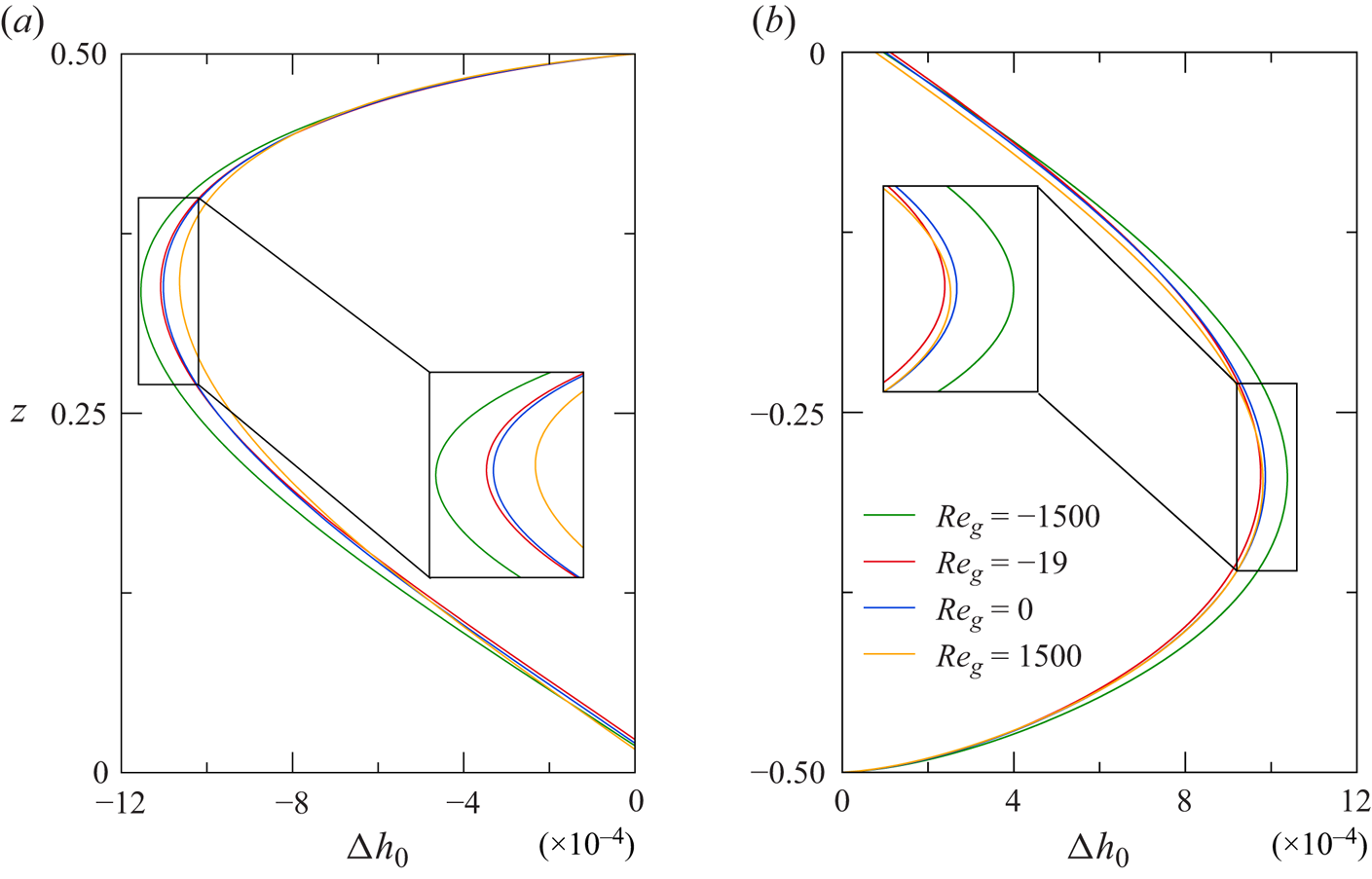
Figure 22. Dynamic surface deformations  $\Delta h_0$ for
  ${Re}=1700$ and different
  ${Re}_{g}$ with an enlarged view of the black rectangle: (a) upper half of the liquid bridge
  $z \in [0;0.5]$; (b) lower half of the liquid bridge
  $z \in [-0.5; 0]$.
For heating from below  $({Re}<0)$ the dynamic surface deformation due to the thermocapillary flow and that due to the gas flow have comparable magnitudes. This leads to qualitatively different dynamic surface deformation profiles as compared with heating from above. This is demonstrated in figure 23(a) for heating from below with
  ${Re}=-1700$ and different gas flow rates in the range
  ${Re}_{g}\in [-3500,1500]$. For a weak heating from below with
  ${Re}=-100$, a strong gas flow from above leads to a bulging near the hot and the cold corner, where the two relative maxima arise with comparable magnitudes. Figure 23(b) shows typical profiles for
  ${Re}\approx -1605$ at which the locus
  $z_{max}$ of
  $\Delta h_{0,max}$ makes a jump. Comparing figures 22(a) and 23(a), we note that
  $\Delta h_0$ is considerably more sensitive to the strength of the gas flow when heating from below as compared with heating from above.

Figure 23. Dynamic surface deformations  $\Delta h_0$ for
  ${\mathcal {V}}=1$, normal gravity (
 $1g$) and different
  ${Re}_{g}$ as indicated. Heating is from below with (a)
  ${Re}=-1700$ and (b)
  ${Re}=-100$.
The vertical coordinate  $z_{max}$ at which the maximum surface deformation
  $\Delta h_{0,max}$ arises is shown in figure 24 as a function of the gas flow Reynolds number
  ${Re}_{g}$ for
  ${\mathcal {V}}=1$ and normal gravity (
 $1g$). The black lines correspond to the projected black lines in figure 19 for
  ${Re}=0$, taking into account the gas flow alone. The effect of the thermocapillary-buoyant flow on
  $z_{max}$ is shown by coloured lines for different values of
  ${Re}$. For heating from above (full coloured lines), we observe a small smooth wiggle near
  ${Re}_{g}\approx 0$ that is related to the already discussed transition from the conductive to the convective regime in the gas phase. In addition, for small Reynolds numbers
  $0<{Re}\leq 50$ (blue and red full lines) a strong gas flow from below sizably affects
  $z_{max}$, because the dynamic deformations due to the thermocapillary and the gas flow are of comparable magnitude, but of different shape. For heating from below (coloured dashed lines), the locus
  $z_{max}$ makes a jump from near the upper cold wall to near the lower hot wall when the cold counter-flow is intensified. For
  ${Re}=-100$ this jump occurs near
  ${Re}_{g}\approx -1605$, as illustrated in figure 23(b). The stronger the thermocapillary flow (the larger
  $|{Re}|$), the stronger the cold downward counter-flow of the gas
  $({Re}_{g} < 0)$ must be for the maximum bulging to occur on the lower (hot) side of the liquid bridge.

Figure 24. Axial position  $z_{max}$ of the maximum dynamic surface deformation
  $\Delta h_{0,max} = \max _z (\Delta h_0 )$ for
  ${\mathcal {V}}=1$ and normal gravity (
 $1g$) as function of
  ${Re}_{g}$ for several
  ${Re}$ (indicated by colour and line type).
4.2.4. Linear stability of the basic flow with a dynamically deformed free surface
The linear stability boundary for a static interface  ${Re}_{c,s}$ as function of the gas flow rate
  ${Re}_{g}$ for heating from above and from below has been presented in figure 2(a). Since the dynamic deformations are small, they are expected to have only a weak influence on the linear stability boundary. This was already noticed for the test case considered during the code validation (figure 33) in Appendix C.4.
Two regions within which the critical Reynolds number for a static interface  ${Re}_{c,s}({Re}_{g})$ deviates the most from that for a dynamically deformed interface
  ${Re}_{c,d}({Re}_{g})$ are shown in figure 25. To quantify the small difference between the two critical curves we define the deviations
 $$\begin{gather} \hat{\epsilon}({Re}_{g}) := {Re}_{c,d}({Re}_{g})-{Re}_{c,s}({Re}_{g}), \end{gather}$$
 $$\begin{gather}\check{\epsilon}({Re}) := {Re}_{g}^{c,d}({Re})-{Re}_{g}^{c,s}({Re}), \end{gather}$$
where  ${Re}_{g}^{c,d}$ and
  ${Re}_{g}^{c,s}$ are the critical gas Reynolds numbers for given
  ${Re}$ and dynamic and static interface, respectively. The meaning of
  $\hat {\epsilon }$ and
  $\check {\epsilon }$ is graphically indicated in figure 25. We also define the relative deviation
 \begin{equation} \hat{\hat{\epsilon}}({Re}_{g}) := \frac{\hat{\epsilon}({Re}_{g})}{{Re}_{c,s}({Re}_{g})}. \end{equation}
We do not define the corresponding relative deviation  $\check {\check {\epsilon }}({Re})$, because the normalising denominator
  ${Re}_{g}^{c,s}({Re})$ would vanish at the critical point
  ${Re}={Re}_{c,s}({Re}_{g}=0)$, i.e. for a closed container. The deviations
  $\hat {\hat {\epsilon }}$ (blue) and
  $\check {\epsilon }$ (red) are shown in figure 26 over the full range of gas Reynolds numbers considered, where
  $\check {\epsilon }({Re})$ is evaluated as
  $\check {\epsilon }[{Re}_{c,s}({Re}_{g})]$. Naturally,
  $\hat {\hat {\epsilon }}$ becomes largest when the slope of the critical curve
  $\partial {Re}_{c,s}/\partial {Re}_{g}\to \infty$ diverges. The deviation of
  $\hat {\hat {\epsilon }}$ at such points, which is also illustrated in figure 25(a) for
  ${Re}_{g}=-1921$, can be larger than 10 %. Similarly,
  $\check {\epsilon }$ becomes large at extrema of the critical curve, i.e. when
  $\partial {Re}_{c,s}/\partial {Re}_{g}\to 0$. An example is shown in figure 25(b) for
  ${Re}_{g}=-424$. Near extrema of
  ${Re}_{c,d}$ the deviation normal to the critical curve represents the meaningful measure. From figure 26, the relative deviation
  $\hat {\hat {\epsilon }}$ typically amounts to a few percent, except possibly at the mentioned extrema. Since the deviation
  $\hat {\hat {\epsilon }}$ can take positive and negative signs for either heating direction, the dynamic surface deformation can act slightly stabilising or slightly destabilising. The absolute deviation
  $\check {\epsilon }$ is typically less than 25, a value which must be compared with the gas Reynolds number which varies over a much wider range
  $(O(10^3))$. The weak effect of a dynamically deformable interface in the basic flow on the stability boundary is also reflected in the minute displacement of the codimension-two points listed in table 4.

Figure 25. Critical Reynolds numbers for  ${\mathcal {V}}=1$ and normal gravity (
 $1g$). Shown are
  ${Re}_{c,s}$ (blue, static interface) and
  ${Re}_{c,d}$ (red, dynamic deformable interface) for heating from above and (a)
 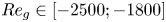 ${Re}_{g} \in [-2500; -1800]$ and (b)
 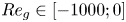 ${Re}_{g} \in [-1000; 0]$. The deviation
  $\hat {\epsilon }$ and
  $\check {\epsilon }$ between the two critical curves are defined graphically in (a).
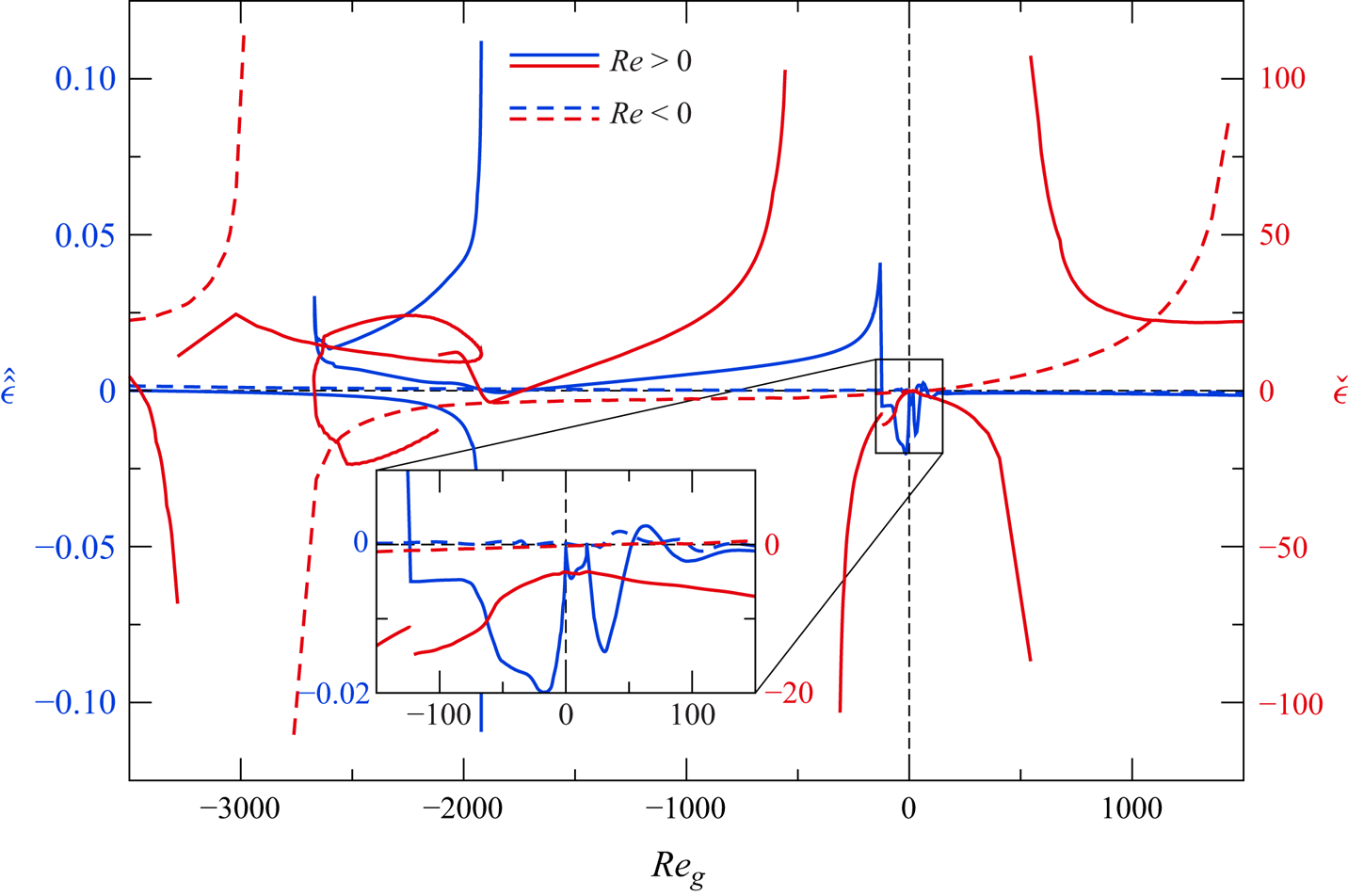
Figure 26. Relative deviation of the critical Reynolds number  $\hat {\hat {\epsilon }} = ({Re}_{c,d} - {Re}_{c,s}) / {Re}_{c,s}$ (blue lines) and absolute deviation of the critical gas Reynolds number
  $\check {\epsilon } = {Re}_{g}^{c,d}({Re}) - {Re}_{g}^{c,s}({Re})$ (red lines), both as functions of
  ${Re}_{g}$. Full and dashed lines correspond to heating from above
  $({Re}_c > 0)$ and from below
  $({Re}_c < 0)$, respectively.
5. Summary and conclusions
The thermocapillary flow in a liquid bridge made from 2-cSt silicone oil  $({Pr} = 28)$ has been investigated for heating from above and from below under axial gravity. The thermal and mechanical coupling between the liquid bridge and the surrounding air is fully accounted for, including the hydrostatic shape of the liquid–gas interface and its flow-induced dynamic deformation. The flow in the liquid is driven by three mechanisms: (a) the thermocapillary stress on the liquid–gas interface, (b) buoyancy forces in the bulk and (c) an axial gas flow imposed on the annular inlet of the gas space which is confined between the liquid bridge and an out shield cylinder. Thermocapillary and buoyancy forces (a) and (b) depend on the applied temperature difference, while the gas flow (c) can be imposed independently. The steady axisymmetric multiphase flow problem is solved numerically, fully taking into account the dependence of the density on the temperature. Thereafter, this basic flow is analysed with respect to its linear stability.
The linear stability boundary of the axisymmetric flow for  ${Pr}=28$ and
  ${\mathcal {V}}=1$ has been established as a function of the gas flow rate, which can take positive or negative values, and for both heating from above and from below. Throughout, the instability is due to hydrothermal waves (Smith & Davis Reference Smith and Davis1983a; Wanschura et al. Reference Wanschura, Shevtsova, Kuhlmann and Rath1995; Stojanovic et al. Reference Stojanović, Romanò and Kuhlmann2022). The waves can have different wavenumbers and exhibit different structures. For a moderate gas flow the linear stability boundary depends sensitively on the imposed gas flow in the range of gas flow Reynolds numbers
 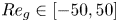 ${Re}_{g}\in [-50, 50]$. This sensitivity was noted before by Kamotani, Chang & Ostrach (Reference Kamotani, Chang and Ostrach1996), Kamotani et al. (Reference Kamotani, Wang, Hatta, Wang and Yoda2003) and, more recently, by Yano et al. (Reference Yano, Maruyama, Matsunaga and Nishino2016) and Gaponenko et al. (Reference Gaponenko, Mialdun, Nepomnyashchy and Shevtsova2021). The sensitivity results from the heating or cooling of the free surface due to the gas flow such that the plateau temperature near midplane changes. This affects the strength and structure of the basic vortex and, thus, the basic temperature field from which the hydrothermal wave extracts its energy. These changes modify the energy supply to the temperature field of the hydrothermal wave via the advection of basic state temperature by the perturbation flow. Typically, radial advection of basic state temperature is by far the most important instability mechanism. The heat exchange through the free surface between the liquid and the gas due to the perturbation flow itself is unimportant.
For larger gas flow rates, but still within  ${Re}_{g}\in [-3500, 1500]$, the linear stability boundary approximately saturates, independent of its direction. In all cases, the reason for the saturation of the critical Reynolds number is an insensitivity of the flow and temperature field inside the liquid phase with respect to an increase of the gas flow rate. The critical thermocapillary Reynolds number for large gas flow rates is of the order of
  ${Re}_c=O(500)$, except for heating from below and a hot co-flow of the gas, for which the stability boundary saturates at
  ${Re}_c=O(1800)$. The saturation of the critical Reynolds number is reached monotonically with an increase of the strength of the gas flow, except for heating from above and a hot co-flow of the gas. In this case the basic flow is very stable up to about
  ${Re}_c\approx 2000$ in the range approximately
  ${Re}_{g}\in [-2000,-100]$ before saturation occurs for
  ${Re}_{g} \lesssim -2000$. In the range
  ${Re}_{g} \in [-2672,-1921]$ and heating from above the linear stability boundary is not unique. Therefore, the unstable basic flow is possibly stabilised again at higher Reynolds numbers within a certain range of
  ${Re}$. In the full range of gas flow rates considered the mechanical driving of the flow in the liquid phase by viscous stresses on the interface exerted by the gas motion is insignificant.
The linear stability boundaries have been computed for a constant volume fraction  ${\mathcal {V}}=1$ and a liquid–gas interface which is statically determined by the mean surface tension and by the hydrostatic pressure. In addition, the stability boundaries have been computed taking into account the flow-induced dynamic interface deformation due to the basic flow, while neglecting the dynamic deformation due to the perturbation flow. Dynamic deformations of the interface are caused by the variation of the surface tension with temperature, viscous normal stresses from the gas and the liquid, and by the dynamic pressure in the gas and the liquid. The dynamic deformation of an isothermal liquid bridge caused by the gas flow alone was found to be consistent with the pressure distribution in the gas near the interface. The distribution of the pressure in the gas is mainly determined by the shape of the static interface and the corner singularities which arise in the gas flow when the liquid contact angle is less than
  ${\rm \pi} /2$. For non-isothermal liquid bridges and heating from above the dynamic surface deformation due to the thermocapillary forcing is typically dominant over the gas-flow-induced deformation and leads to a sinusoidal dynamic deformation supporting bulging near the cold wall and necking near the hot wall, superimposed to the static shape. But for heating from below, the dynamic deformation due to the thermocapillary flow can have the same order of magnitude as that due to the gas flow (for comparable Reynolds numbers). Therefore, the shape of the dynamic deformation can be more complicated. Regardless of the shape of the dynamic surface deformation, its effect on the critical threshold is weak.
With the present study we have accurately established the dependence on a forced gas flow of the linear stability boundary of the axisymmetric thermocapillary flow in liquid bridge of  ${Pr}=28$. We have incorporated in the analysis static and dynamic interface deformations, the presence of a gas phase, a forced flow in the gas phase, and non-Oberbeck–Boussinesq effects due to the linear dependence of the density on temperature in all terms. Even though the Bond number was considered constant, the analysis should guide the interpretation of data measured or computed in future investigations of similar flow problems.
As was already pointed out by Shevtsova et al. (Reference Shevtsova, Gaponenko, Kuhlmann, Lappa, Lukasser, Matsumoto, Mialdun, Montanero, Nishino and Ueno2014), the sensitivity of the critical onset of three-dimensional hydrothermal wave on the flow rate and direction of the hot or cold gas bares the potential to controlling the critical onset of flow oscillations. Their linear stability boundaries for 5-cSt silicone oil,  $\eta =2$ and zero gravity (figure 7 of Shevtsova et al. Reference Shevtsova, Gaponenko, Kuhlmann, Lappa, Lukasser, Matsumoto, Mialdun, Montanero, Nishino and Ueno2014) are similar to the present stability boundaries (figure 2a) for heating from above: a very stable basic flow for a certain range of
  ${Re}_{g} < 0$ and an approximate saturation of
  ${Re}_c$ for
  ${Re}_{g}>0$. The details, however, are more complicated. In particular, we did not find the stationary
  $m_c=1$ mode at very low Reynolds number of the order of 200 for
  ${Re}_{g}>0$. This may partly be related to the relatively tight air gap with
  $\eta =2$ considered by Shevtsova et al. (Reference Shevtsova, Gaponenko, Kuhlmann, Lappa, Lukasser, Matsumoto, Mialdun, Montanero, Nishino and Ueno2014). Probably for the same reason, the two-dimensional instability found for
  $\eta =1.\bar 6$ by Shevtsova et al. (Reference Shevtsova, Gaponenko and Nepomnyashchy2013) for
  ${Re}_{g} > 0$ does not arise in the present system. We also did not find indications for a classical Marangoni instability (different from Shevtsova et al. Reference Shevtsova, Gaponenko and Nepomnyashchy2013), even though the production of thermal perturbation energy is dominated by radial advection of basic state temperature
  $(J_1)$: The region below the free surface in the plateau region of the surface temperature profile is found to be almost isothermal. For the Pearson mechanism (Pearson Reference Pearson1958) to arise the basic temperature field should exhibit a significant temperature gradient next to the interface. However, for the range of parameters investigated, as in the classical hydrothermal wave (Wanschura et al. Reference Wanschura, Shevtsova, Kuhlmann and Rath1995), the radial temperature gradients arise only deep inside the liquid bridge due to the return flow of the basic toroidal vortex which is absent in the Pearson problem.
Owing to the large parameter space, other important influence factors have not been included in the present analysis. Among these are the dependence of the viscosity on the temperature (Kozhoukharova et al. Reference Kozhoukharova, Kuhlmann, Wanschura and Rath1999; Shevtsova, Melnikov & Legros Reference Shevtsova, Melnikov and Legros2001) and evaporative cooling for large  $\Delta T$ (Simic-Stefani, Kawaji & Yoda Reference Simic-Stefani, Kawaji and Yoda2006; Yano et al. Reference Yano, Maruyama, Matsunaga and Nishino2016). In addition, an extension of the analysis to other Prandtl numbers and volume fractions of the liquid would be of interest. With respect to future space experiments which allow for larger liquid bridges it would also be desirable to take into account dynamic surface deformations in the perturbation flow. The would allow for surface wave instabilities which have been found to become critical for pure thermocapillary flow in plane layers of low Prandtl number (Smith & Davis Reference Smith and Davis1983b) and in flat migrating droplets (Hu et al. Reference Hu, Zhang and Chen2023). At higher gas flow rates, for which the shape of the liquid bridge is sizably affected by dynamic deformations, surface waves can also be triggered by the Kelvin–Helmholtz mechanism. These effects suggest corresponding extensions of the present work.
Funding
This work has been supported by the Austrian Research Promotion Agency (FFG) in the framework of the ASAP14 programme under contract number 866027. Open Access of this paper has been funded by TU Wien Bibliothek.
Declaration of interests
The authors report no conflict of interest.
Author contributions
All authors contributed equally to analysing data and reaching conclusions, and in writing the paper.
Appendix A. Reynolds number for the gas motion
The motion of the gas resembles the flow through an annular pipe for which the Reynolds number is usually defined as  ${Re}_{g}'=2\bar {w}_{g,in} \rho _{g0} (r_{o}-r_{i})/\mu _{g}$, based on the kinematic viscosity of the gas and the width of the annular gap. In the thermocapillary liquid bridge under investigation, however, the flow instability is triggered in the liquid phase, while the gas phase is mainly passive. Therefore, the effect of the gas motion on the liquid phase is better represented by using the kinematic viscosity of the liquid
  $\mu /\rho _0$ and the length scale
  $d$ of the liquid phase, leading to
  ${Re}_{g}=\bar w_{g,in}d\rho _0/\mu$. Both Reynolds numbers are related to each other by
 \begin{equation} {Re}_{g}' = \frac{2(\eta -1)}{\varGamma} \frac{\tilde{\rho}}{\tilde{\mu}} {Re}_{g} , \end{equation}
through the ratio of the kinematic viscosities  $\tilde {\rho }/\tilde {\mu }$ and twice the ratio of the length scales
  $2(\eta -1)/\varGamma$.
The relevance of  ${Re}_{g}$ for the flow instability can also be inferred from table 5 which shows the critical thermocapillary Reynolds number
  ${Re}_{c,d}$ when the liquid–gas interface of the basic state is dynamically deformable (subscript
  $d$). Based on the reference case (Ref) for
  ${Re}_{g}=-40$ and
  ${Re}_{g}'=-46.65$, we consider the deviation of the critical Reynolds number
  $\hat \delta ={Re}_c-{Re}_c^{ref}$ from the reference value
 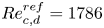 ${Re}_{c,d}^{ref}=1786$ when the dimensional radius of the gas tube
  $r_{o}$, and thus the gap width
  $\eta$, is varied. Keeping
  ${Re}_{g}$ constant (data shown in blue) the critical Reynolds numbers deviate much less from the reference value than when
  ${Re}_{g}'$ is kept constant (data shown in red). For that reason we used
  ${Re}_{g}$ to characterise the strength of the gas flow.
Table 5. Critical thermocapillary Reynolds number  ${Re}_{c,d}$ for different tube radii
  $r_{o}$ and mean inlet velocities
  $\bar w_{g,in}$ under zero gravity. The remaining parameters correspond to the reference parameters specified in § 4. Also given are the gas flow Reynolds numbers
  ${Re}_{g}'$ and
  ${Re}_{g}$ and the percentage deviation
  $\hat \delta$ of the critical Reynolds number from the one for the reference case (denoted ‘Ref’). Equal values of
  ${Re}_{g}'$
  $({Re}_{g})$ are shown in red (blue).
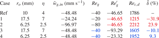
Appendix B. Dependence of the critical Reynolds number on the rod length $\varGamma _{rod}$

The temperatures at the in- and outlet of the gas space as well as the inlet velocity profile are prescribed. To estimate the length  $l$ over which the downstream boundary conditions affect the velocity field upstream the equilibrium between momentum advection and diffusion over the influence length
  $l$ can be estimated by the condition
 \begin{equation} {Pe} = \frac{\bar w_{g,in} \rho_{g0} l}{\mu_{g}} \approx 1 \end{equation}
for the Péclet number  ${Pe}$. Expressed by the gas flow Reynolds number
  ${Re}_{g}$, this yields
 \begin{equation} \frac{l}{d} \approx \frac{\tilde \mu}{\tilde\rho {Re}_{g}} \approx \frac{7.8}{{Re}_{g}}. \end{equation}
Thus, in order that the dimensionless influence length  $l/d$ is less than the dimensionless rod length
 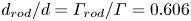 $d_{rod}/d = \varGamma _{rod}/\varGamma = 0.606$, the gas flow Reynolds number should satisfy
  $|{Re}_{g}|\gtrsim 13$. With
  ${Pr}_{g} =\mu _{g}c_{p{g}}/\lambda _{g}= 0.704$ a similar estimate,
 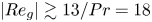 $|{Re}_{g}|\gtrsim 13/{Pr} = 18$, holds for the thermal influence length. Thus, the critical Reynolds number should not be affected by the relatively short length of the rods with
  ${\varGamma _{rod}=0.4}$, except for very small gas flow rates.
This is confirmed by figure 27 which shows the critical Reynolds number as a function of  $\varGamma _{rod}$ is independent of
  $\varGamma _{rod}$ for
  $\varGamma _{rod}>0.4$ and
  ${Re}_{g}=\pm 500$ with heating from above (full lines) and heating from below (dashed lines). The deviations of
  ${Re}_c(\varGamma _{rod}=0.4)$ from
  ${Re}_c(\varGamma _{rod}=8)$ are less than 1 %. Even for
  ${Re}_{g} =0$ and heating from above independence from
  $\varGamma _{rod}$ is achieved for
  $\varGamma _{rod}\gtrsim 0.5$ with
  ${Re}_c(\varGamma _{rod}=0.4)$ deviating from
  ${Re}_c(\varGamma _{rod}=8)$ by less than 8 %. For
  ${Re}_{g} =0$ and heating from below, however, the critical Reynolds number exhibits a strong dependence on
  $\varGamma _{rod}$ with changes of the critical mode (dashed orange lines in figure 27). The critical mode for small
  $\varGamma _{rod}$ is due to a hydrothermal wave in the liquid with
  $m_c=2$ (see figure 2a). The critical mode changes at
  $\varGamma _{rod}= 1.77$ to a stationary mode with
  $m_c=2$ which is triggered in the gas phase. At
  $\varGamma _{rod}= 2.85$ a further change is found to another stationary mode with
  $m_c=1$. Since the latter instabilities were the only ones found where the flow becomes unstable in the gas phase, the instability for
  $\varGamma _{rod}=8$ is briefly described.

Figure 27. Dependence of the critical Reynolds numbers  ${Re}_{c,d}$ for
  ${\mathcal {V}}=1$ and
  $1g$ on the dimensionless rod length
  $\varGamma _{rod}$ for
  ${Re}_{g} \in \{-500;\, 0;\, 500\}$ and heating from above (full lines) and heating from below (dashed lines). The grey stripes indicate an error of
  $\pm$5 % with respect to
  ${Re}_{c,d}(\varGamma _{rod}=8)$. The vertical dotted line marks the rod aspect ratio
  $\varGamma _{rod}=0.4$ employed.
The critical Reynolds number for  $\varGamma _{rod}=8$ is
  ${Re}_c=-146$ (corresponding to
  $\Delta T_c=-4.4$ K). The basic state and a cross-section of the critical mode are shown in figure 28. The critical mode involves a large-scale circulation in the full annular gas space (figure 28b). The air rises on one side of the annular pipe and descends on the other side. The critical velocity and temperature fields in the liquid are much weaker than in the gas phase. Obviously, the instability is due to buoyancy. To estimate the magnitude of the buoyancy in the gas phase we evaluate the Rayleigh number in the gas based on the height of the gas tube. For the present reference parameters the Rayleigh number is
 \begin{equation} {Ra}_{g} = \frac{\tilde{\rho}^2\tilde\beta\tilde{c}_p}{\tilde{\mu}\tilde{\lambda}} \left(1+2\frac{\varGamma_{rod}}{\varGamma}\right)^3 {Pr}{Bd}{Re} \approx 1.30\times 10^{{-}2} (1+3.03\times \varGamma_{rod})^3 {Re}. \end{equation}
For the rod aspect ratio  $\varGamma _{rod}=8$ and for
  $|{Re}| = |{Re}_{c,d}(\varGamma _{rod}=8)| = 146$, the Rayleigh number is
  ${Ra}_c = {Ra}({Re}_{c,d}) \approx 30\,500$ which is of the same order of magnitude as the critical value of
  ${Ra}_c\approx 51\,000$ according to the correlation of D'Orazio, Cianfrini & Corcione (Reference D'Orazio, Cianfrini and Corcione2004) for the onset of convection in a rectangular two-dimensional container heated from below with adiabatic sidewall and the same aspect ratio
  $(d+2d_{rod})/(r_{o} - r_{i})=5.55$.

Figure 28. (a) Basic state at criticality  ${Re}_{c,d}=-146$ for
  $\varGamma _{rod}=8$,
  ${\mathcal {V}}=1$,
  $1g$,
$1g$,  ${Re}_{g}=0$ and heating from below. (b) Corresponding stationary critical mode with
  $m=1$, shown in the plane
  $\varphi =\textrm {const.}$ in which the local thermal energy production has its maximum.
The presence of the buoyant instability in the gas phase shows that the above estimate based on advection and diffusion is incomplete to estimate the effect of  $\varGamma _{rod}$ in the presence of gravity. Therefore, we compare in figure 29 the neutral curves
  ${Re}_n({Re}_{g})$ for
  $\varGamma _{rod}=0.4$ (dashed lines) with those for
  $\varGamma _{rod}=8$ (full lines) for both heating from above (red curves) and below (blue curves). For sufficiently strong gas flow, the rod aspect ratio (up to
  $\varGamma _{rod}=8$) does not significantly affect the instability. For weak gas flow in the range
  ${Re}_{g}\in [-80,20]$ and for heating from below (blue lines,
  ${Re}_{n,d}<0$), however, stationary buoyant instabilities (as in figure 28) can arise in the gas phase and break the axisymmetry before hydrothermal waves become unstable.

Figure 29. Neutral Reynolds numbers as functions of  ${Re}_{g}$ for
  $\varGamma _{rod}=0.4$ (dashed lines) and
  $\varGamma _{rod}=8$ (full lines). Results are shown for heating from above (red lines, left axis) and for heating from below (blue lines, right axis,
  ${Re}_{n,d}<0$). The neutral wavenumbers
  $m=1$,
  $m=2$ and
  $m=3$ are indicated by labels. The grey region indicates a deviation of
  $\pm$2 % with respect to the neutral curves for
  $\varGamma _{rod}=8$. The blue square indicates the conditions of figure 28.
Considering  $\varGamma _{rod}=8$ sufficiently large to suppress effects due to the inlet and outlet length on the basic flow, we define a tolerance of
  $\pm$2 % for the critical Reynolds number for hydrothermal waves (grey shaded region in figure 27). Comparing
  ${Re}_{c,d}(\varGamma _{rod}=0.4)$ (dashed lines) with
  ${Re}_{c,d}(\varGamma _{rod}=8)$ (full lines), we find that using
  $\varGamma _{rod}=0.4$ provides a good approximation of the critical Reynolds number for hydrothermal waves in the axially extended system with
  $\varGamma _{rod}=8$, if
  $|{Re}_{g}|>17$ in the case of heating from below (blue lines). For heating from above (red lines) the restriction is similar with
  ${Re}_{g}>21$ for hot downward co-flow, whereas for cold upward counter-flow the restriction is more severe and
  ${Re}_{g} < -90$ must be satisfied. Since the length of the support rods in typical experiments is limited and the heating is usually from above, buoyant instabilities such as that shown in figure 28 do not arise. Therefore,
  $\varGamma _{rod}=0.4$, also employed by Romanò et al. (Reference Romanò, Kuhlmann, Ishimura and Ueno2017), is a reasonable choice for the length of the support rods, if one keeps in mind that the critical Reynolds numbers for weak gas flows depends on
  $\varGamma _{rod}$.
Appendix C. Verification and validation of the dynamic surface deformation
To check the implementation of dynamic free-surface deformation the surface shapes obtained using the code MaranStable are compared with available experimental and numerical results. Some comparisons are made for the single-fluid model in which viscous stresses from the gas phase are absent. In most tests a quantitative agreement is found.
C.1. Comparison with Kuhlmann & Nienhüser (Reference Kuhlmann and Nienhüser2002)
Kuhlmann & Nienhüser (Reference Kuhlmann and Nienhüser2002) have carried out an asymptotic expansion of the thermocapillary flow and interface shape for the limit  ${Ca} \to 0$. The same approach was used by Shevtsova et al. (Reference Shevtsova, Mialdun, Ferrera, Cabezas and Montanero2008). For a comparison with the results of Kuhlmann & Nienhüser (Reference Kuhlmann and Nienhüser2002) we consider a liquid bridge with
  $\varGamma =1$,
  ${\mathcal {V}}=1$, an adiabatic free surface, zero gravity and a Capillary number
  ${Ca}=10^{-6}$. Under zero gravity
  ${({Bd}={Bo}=0)}$ the static shape is cylindrical with
  $h_{0,s}(z)\equiv 1/\varGamma$. Figure 30 shows the deviation
  $\Delta h_0$ of the surface shape from cylindrical obtained by MaranStable (lines) in comparison with the first-order correction
  $h^{(1)} {Ca}$ to the cylindrical shape computed by Kuhlmann & Nienhüser (Reference Kuhlmann and Nienhüser2002) (dots) for different combinations of
  ${Re}$ and
  ${Pr}$. Our results agree very well with the literature data, particularly for the viscous–conductive case
  ${Re}=10^{-4}$,
  ${Pr}=0.02$ (blue). Deviations among the two results slightly increase for larger Marangoni numbers, i.e. for
  ${Re}=2130$,
  ${Pr}=0.02$ (red, near the hot wall at
  $z=1/2$) and for
  ${Re}=951$,
  ${Pr}=4.38$ (orange near the midplane). A plausible reason for these minor deviations is the absence of higher-order corrections in
  ${Ca}$ of the interface shapes provided by Kuhlmann & Nienhüser (Reference Kuhlmann and Nienhüser2002).
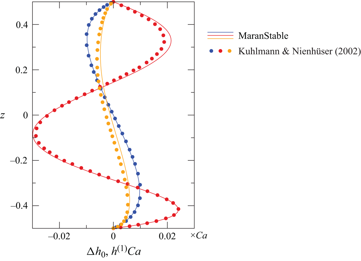
Figure 30. Comparison of the scaled dynamic surface deformations  $\Delta h_0$ (lines) with the first-order correction
  $h^{(1)} {Ca}$ of Kuhlmann & Nienhüser (Reference Kuhlmann and Nienhüser2002) (dots, taken from their figure 2a) for
  $\varGamma =1$,
  ${\mathcal {V}}=1$,
 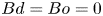 ${Bd}={Bo}=0$,
  ${Ca}=10^{-6}$, adiabatic free surface and
  $({Pr},{Re})=(0.02,10^{-4})$ (blue),
  $(0.02,2130)$ (red) and
  $(4.38,951)$ (orange). Viscous stresses from the gas phase are neglected.
C.2. Comparison with Montanero et al. (Reference Montanero, Ferrera and Shevtsova2008)
To validate the dynamic deformations obtained by MaranStable for larger dynamic surface deformations we also compare with the experimental results obtained by Montanero et al. (Reference Montanero, Ferrera and Shevtsova2008). While the experimental data are obtained in the presence of the gas phase, it is neglected in our calculations. The reason is Montanero et al. (Reference Montanero, Ferrera and Shevtsova2008) did not provide any information about the ambient gas and the complimentary numerical computations by Carrión et al. (Reference Carrión, Herrada and Montanero2020) were made for a single-fluid model. Following Carrión et al. (Reference Carrión, Herrada and Montanero2020) we assume the thermal boundary condition can be modelled by Newton's law of cooling
 \begin{equation} \boldsymbol{n}\boldsymbol{\cdot}\boldsymbol{\nabla}\vartheta ={-}{Bi} \left(\vartheta+\tfrac{1}{2}\right), \end{equation}
with a Biot number  ${Bi}=h_q d/\lambda =0.15$, where
  $h_q$ is the heat-transfer coefficient between the liquid and the gas.
We consider a liquid bridge of length  $d=3.69$ mm made from 5-cSt silicone oil
  $({Pr}=67)$ for
  $\varGamma = 1.23$ and
  ${\mathcal {V}} = 0.82$ (underfilling) under normal gravity and heated from above. Figure 31(a) shows the static surface shape computed using MaranStable. The horizontal axes show both the dimensional
  $(h_{0,s}-r_{i})$ and the non-dimensional deviation
  $(h_{0,s}-1/\varGamma )$ of the static surface shape from cylindrical. The (additional) flow-induced dynamic deformation
  $\Delta h_0 = h_{0,d} - h_{0,s}$ is shown in figure 31(b). The results obtained with MaranStable are in a reasonable agreement with the experimental data.

Figure 31. (a) Static surface shape  $h_{0,s}$ of a tall liquid bridge made from 5-cSt silicone oil under normal gravity with length
  $d=3.691$ mm, aspect ratio
  $\varGamma = 1.23$ and volume
  ${\mathcal {V}} = 0.82$. (b) Dynamic surface deformation
  $\Delta h_0$ for the same liquid bridge for
  $\Delta T = 11.05$ K (
 ${Re} = 113.9$, blue) and
  $\Delta T = 21.76$ K (
 ${Re} = 224.4$, red). Lines show results of MaranStable, while squares represent experimental data of Montanero et al. (Reference Montanero, Ferrera and Shevtsova2008). The experimental error bars (
 $\pm$1
  $\mathrm {\mu }$m) were estimated by Montanero et al. (Reference Montanero, Ferrera and Shevtsova2008).
Deviations between our numerical results (lines) and the experimental data (solid squares) are expected. Notwithstanding the measurement error, the heat flux through the interface is not correctly described by (C1) when using a constant Biot number (Romanò & Kuhlmann Reference Romanò and Kuhlmann2019).
C.3. Comparison with Matsunaga et al. (Reference Matsunaga, Mialdun, Nishino and Shevtsova2012)
Dynamic surface deformations arise not only due to a temperature gradient along the interface, but also due to viscous shear stresses from the gas phase. To test the dynamic surface deformation caused solely by an axial gas flow, we also compare with the experimental results of Matsunaga et al. (Reference Matsunaga, Mialdun, Nishino and Shevtsova2012). Again, we consider a liquid bridge of 5-cSt silicone oil, but with nitrogen as the ambient gas. Moreover, the geometry of the set-up was adapted to that of Matsunaga et al. (Reference Matsunaga, Mialdun, Nishino and Shevtsova2012) by selecting  $\varGamma =1$,
  $\varGamma _{rod}=2/3$ and
  $\eta =5/3$. The liquid bridge of length
  $d=3$ mm and relative volume
  ${\mathcal {V}}=0.8$ is isothermal, and the gas enters the shield tube from below (
 ${Re}_{g}> 0$).
Figure 32(a) shows the deviation  $h_{0,s}-1/\varGamma$ of the static shape from cylindrical. The flow-induced dynamic part of the deformation
  $\Delta h_0 = h_{0,d} - h_{0,s}$ is shown in figure 32(b) for
  ${Re}=0$. Shown are profiles computed by MaranStable for
  ${Re}_{g}=600$ (blue line), 900 (red line) and 1200 (orange line). For
  ${Re}_{g}=600$ and 900 an excellent agreement is found with the corresponding experimental results (symbols).
Figure 32. (a) Deviation  $h_{0,s}-1/\varGamma$ of the static interface shape from cylindrical for a liquid bridge of length
  $d=3$ mm made from 5-cSt silicone oil in nitrogen. The essential non-dimensional parameters are:
  $\varGamma = 1$,
  ${\mathcal {V}} = 0.8$,
  ${Bo}=4.075$ (ground condition) and
  ${Re}=0$ (see the text for the remaining geometry parameters).(b) Dynamic part of the interfacial deformation
  $\Delta h_0$ computed using MaranStable (lines) in comparison with the measurements of Matsunaga et al. (Reference Matsunaga, Mialdun, Nishino and Shevtsova2012) (squares) for different through flows:
  $\bar w_{g,in} = 1$ m s
 $^{-1}$ (
 ${Re}_{g} = 600$, blue),
  $\bar w_{g,in} = 1.5$ m s
 $^{-1}$ (
 ${Re}_{g} = 900$, red) and
  $\bar w_{g,in} = 2$ m s
 $^{-1}$ (
 ${Re}_{g} = 1200$, orange). Error bars show an uncertainty of
  $\pm$0.6
  $\mathrm {\mu }$m.
Even though Matsunaga et al. (Reference Matsunaga, Mialdun, Nishino and Shevtsova2012) estimated the measurement error of  $h_{0,d}$ as
  $\pm$0.1
  $\mathrm {\mu }$m, we show error bars for
  $\pm$0.6
  $\mathrm {\mu }$m. The reason is Matsunaga et al. (Reference Matsunaga, Mialdun, Nishino and Shevtsova2012) found that the deviation between their measured static interfacial shape
  $h_{0,s}$ for
  ${Re}_{g} =0$ and their numerical solution of the Young–Laplace equation (our solution is shown in figure 32a) was
  $\pm$0.6
  $\mathrm {\mu }$m on average, with a maximum deviation of
  $\pm$1.5
  $\mathrm {\mu }$m. Since only the total dynamic shape
  $h_{0,d}$ is observed experimentally, the dynamic part of the deformation
  $\Delta h_0$ is also affected by the error in the static shape
  $h_{0,s}$. This may explain the large deviation between our result and the measured data of Matsunaga et al. (Reference Matsunaga, Mialdun, Nishino and Shevtsova2012) for
  ${Re}_{g}=1200$ (orange in figure 32b).
C.4. Code validation regarding the critical Reynolds number with and without dynamic surface deformation of the basic flow
Finally, we validate MaranStable in terms of the critical onset of three-dimensional flow by comparison with the measurements of Yano et al. (Reference Yano, Maruyama, Matsunaga and Nishino2016) for a liquid bridge of 2-cSt silicone oil in air with length  $r_{i}=d=2.5$ mm and
  ${Pr}=28$,
  ${Bd}=0.41$,
  $\varGamma =1$,
  $\varGamma _{rod}=4.8$ and
  $\eta =5$. Figure 33 shows the neutral and critical Marangoni numbers as functions of the volume ratio
  ${\mathcal {V}}$ for a mean gas inlet velocity of
  $\bar w_{g,in}=-20$ mm s
 $^{-1}$ corresponding to a gas flow Reynolds number of
  ${Re}_{g} = -25$ (cold counter-flow, heating from above,
  $1g$). The numerical neutral curves obtained for a static (
 $h_{0,s}$, dashed lines) and for a dynamic surface shape (
 $h_{0,d}$, full lines) do not deviate much from each other, indicating the weak influence of the dynamic deformability on the critical Marangoni number for such a weak gas flow.

Figure 33. Neutral Marangoni numbers  ${Ma}_n$ (lines) as functions of the volume ratio
  ${\mathcal {V}}$ for a liquid bridge of 2-cSt silicone oil in air with length
  $d=2.5$ mm and
  ${Pr}=28$,
  $\varGamma =1$,
  ${Bd}=0.41$ and
  $\eta =5$. Dashed lines show the static surface shape
  $h_{0,s}$; full lines show the dynamic surface shape
  $h_{0,d}$. A comparison is made with the experimental data of Yano et al. (Reference Yano, Maruyama, Matsunaga and Nishino2016) (their figure 6a) for a gas inlet velocity of
  $-20$ mm s
 $^{-1}$ (
 ${Re}_{g}=-25$). Colour indicates the neutral wavenumber:
  $m=1$ (blue) and
  $m=2$ (red).
Both numerical results are in good agreement with the experimental data for all volume ratios  ${\mathcal {V}}$ sampled. The only exception is the volume
  ${\mathcal {V}}=1.05$ for which the critical wavenumbers deviate qualitatively. Given the experimental error bar, a possible reason could be the large slope of the neutral curve for
  $m=1$ with respect to
  ${\mathcal {V}}$, such that small deviations of
  ${\mathcal {V}}$ cause a large change of the critical Marangoni number. In addition, a subcritical instability at
  ${\mathcal {V}}=1.05$ cannot currently be ruled out.
Appendix D. Verification of the density variation
Different from the Oberbeck–Boussinesq approximation, our code takes into account a linear variation of the density with temperature in all terms. To verify the correct implementation we consider the present standard configuration with  ${Pr}=28$. The liquid bridge is heated from above with
  ${Re}=400$ and exposed to a hot downward flow with
  ${Re}_{g}=200$. In figure 34 we show the volume flow density
  $w_{g}$ (left axis, blue) and the mass flow density
  $\rho _{g} w_{g}$ (right axis, red) as functions of
  $r$ at the in- and outlet. The incoming hot air slows down from an averaged value of
  $\bar {w}_{g}=-0.242$ m s
 $^{-1}$ (full horizontal blue line) to
  $\bar {w}_{g}=-0.233$ m s
 $^{-1}$ (dashed horizontal blue line). As expected, the volume flux cannot be constant and independent of
  $z$, since the gas must have cooled down at the outlet. The total mass flux
  $\dot {m}=\int _A\rho _{g} w_{g}\,\mathrm{d} A$, however, must be independent of
  $z$. The almost invisible discrepancies between the mass flow densities at the inlet (full red curve) and the outlet (dashed red curve) arise, because the gas leaves the tube with a velocity profile which is slightly perturbed due to the thermocapillary flow along the liquid–gas interface. However, the total mass balance long the tube is satisfied up to machine precision: the average mass flow densities
  $\overline {\rho _{g}w_{g}}=-0.281$ [kg m
 $^{-2}$ s
 $^{-1}$] (red horizontal line) deviate by less than
  $10^{-12}$ % from each other.

Figure 34. Volumetric flow rate density (left, blue) and mass flow rate density (right, red) at the inlet (full lines) and at the outlet (dashed lines) of the gas tube for  ${Re}=400$ and a hot downward flow (
 ${Re}_{g}=-200$). The horizontal lines represent averaged values over the cross-section.


 Open access