


1. Introduction
Near-wall turbulence is sustained by the so-called self-sustaining process (SSP); that is, streamwise vortices induce low- and high-speed streaks by the advection of the streamwise momentum, while an instability induces the meandering of streaks leading to the regeneration of streamwise vortices (Hamilton, Kim & Waleffe Reference Hamilton, Kim and Waleffe1995; Waleffe Reference Waleffe1997). It is also known that these quasi-streamwise vortices are inclined in the wall-normal and spanwise directions and they are located in a staggered array (Jeong et al. Reference Jeong, Hussain, Schoppa and Kim1997). When the Reynolds number is low, there is no scale separation and the SSP explains the sustaining mechanism of the turbulence very well.
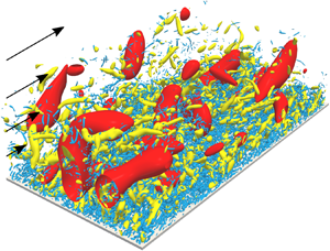
However, as the Reynolds number increases, larger-scale vortices appear in addition to these near-wall coherent vortices. We emphasize that we cannot identify larger-scale vortices in terms of the velocity gradients. For example, the yellow objects in figure 1 are the positive isosurfaces of the second invariant  $Q$ of the velocity gradient tensor in turbulent channel flow at the friction Reynolds number $Re_\tau =u_\tau h/\nu =4179$ (see § 2.1 for the details of the database). Here, $u_\tau$ is the skin-friction velocity and $h$ is the channel half-width. We can only observe the smallest-scale vortices in figure 1. On the other hand, looking at the blue isosurfaces of the fluctuating streamwise velocity, larger-scale motions are prominent. Thus, the quantities related to the velocity are appropriate for extracting the largest-scale structures, whereas those related to its gradients are appropriate for extracting the smallest-scale structures. This is the reason why the velocity has been often used for investigating large-scale motions (LSM). For example, Adrian, Meinhart & Tomkins (Reference Adrian, Meinhart and Tomkins2000) investigated the velocity field in a turbulent boundary layer to show that large-scale hairpin vortices formed packets, which are a kind of LSM. Lee & Sung (Reference Lee and Sung2011) also showed that a packet of hairpin vortices merged the adjacent one, resulting in the creation of very large-scale motions (VLSM). Incidentally, Kevin, Monty & Hutchins (Reference Kevin, Monty and Hutchins2019a) found that large-scale quasi-streamwise vortices exist along the side of large-scale low-speed structures. Thus, since one can easily extract the large-scale structures by visualizing LSM and/or VLSM with the velocity (or the filtered velocity), many authors (e.g. Adrian Reference Adrian2007; Hutchins & Marusic Reference Hutchins and Marusic2007; Monty et al. Reference Monty, Stewart, Williams and Chong2007; Dennis & Nickels Reference Dennis and Nickels2011a,Reference Dennis and Nickelsb; Baltzer, Adrian & Wu Reference Baltzer, Adrian and Wu2013; Lee et al. Reference Lee, Lee, Choi and Sung2014; Lee, Sung & Zaki Reference Lee, Sung and Zaki2017; Kevin, Monty & Hutchins Reference Kevin, Monty and Hutchins2019b) examined large-scale streaky velocity structures and their relation to large-scale vortices.

Figure 1. Vortices and low-speed structures visualized by the isosurfaces of the second invariant ( $Q^{+}=3.0\times 10^{-3}$, yellow) of the velocity gradient tensor and of the streamwise fluctuating velocity ( $\check {u}^{+}=-3$, blue), respectively. The grid width on the wall indicates 1000 wall units. The flow is from lower left to upper right. We visualize a subdomain (half in the spanwise direction and full in the streamwise direction) of the computational domain.
A different approach for extracting multiscale motions in the real space was introduced by Hwang & Cossu (Reference Hwang and Cossu2010), who artificially quenched small-scale motions by using overdamped large-eddy simulations (LES). By examining the coarse-grained fields where small-scale flow structures are absent, Hwang (Reference Hwang2015) showed that energy-containing motions attached to the wall were self-similar. This is a picture consistent with the attached eddy theory (Townsend Reference Townsend1976). These wall-attached structures are composed of streamwise-elongated streaky motions and relatively short vortical structures. Hwang & Bengana (Reference Hwang and Bengana2016) also explored the self-similar nature of the SSP by conducting the overdamped LES in a minimal computational domain.
In our previous study (Motoori & Goto Reference Motoori and Goto2019a), we extracted the hierarchy of multiscale vortices in a turbulent boundary layer by coarse graining the velocity fields obtained by a direct numerical simulation. Since the coarse graining enables us to quantify the interactions among different scales, we evaluated the scale-dependent contributions of the vortex stretching to reveal the generation mechanism of multiscale vortices; vortices as large as the height from the wall are stretched by the mean shear, whereas smaller-scale vortices are stretched by larger-scale vortices. The latter generation mechanism in terms of the vortex stretching is consistent with a picture of the energy cascade in turbulence in a periodic cube (Goto Reference Goto2008, Reference Goto2012; Leung, Swaminathan & Davidson Reference Leung, Swaminathan and Davidson2012; Goto, Saito & Kawahara Reference Goto, Saito and Kawahara2017) and turbulent channel flow at  $Re_\tau = 932$ (Lozano-Durán, Holzner & Jiménez Reference Lozano-Durán, Holzner and Jiménez2016). However, it is not obvious that the process that larger-scale vortices stretch smaller-scale ones corresponds to the energy transfer to smaller scales. This issue was investigated by introducing the scale-dependent energy transfer in the real space (Goto Reference Goto2008, Reference Goto2012) for periodic turbulence, and it was concluded that the energy cascade was the creation of thinner vortex tubes in strongly straining regions around fatter tubes. On the other hand, for wall-bounded turbulence, there are only a few studies of the real-space energy transfer because the quantification of the scale-dependent transfer rate is not straightforward. For example, by using the balance equation of the second-order velocity structure function (a generalized Kolmogorov equation) for turbulent channel flow, Cimarelli et al. (Reference Cimarelli, De Angelis, Jiménez and Casciola2016) examined the energy transfer in the space and scales to show that two types of energy sources caused the complex dynamics of the cascade.
In the present study, we investigate band-pass filtered fields in turbulent channel flow at  $Re_\tau =4179$ (Lozano-Durán & Jiménez Reference Lozano-Durán and Jiménez2014). The Reynolds number of the flow is much higher than in the turbulent boundary layer ( $Re_\tau \approx 1000$) examined in our previous study (Motoori & Goto Reference Motoori and Goto2019a). The purposes of the present study are (i) to show the concrete relation of flow structures (vortices and low-speed regions) at each level of the hierarchy, and (ii) to show the relation between vortex generation processes and the energy cascade, and its similarity in the two wall-bounded turbulent flows. In the rest of the present paper, we first describe in § 2 the numerical database of the turbulent channel flow and the scale-decomposition method. We then examine the different-scale fields to show the hierarchical structures of vortices and streaks (§ 3.1), and their generation mechanisms in terms of the vortex stretching (§ 3.2) and of the real-space energy transfer (§ 3.3).
2. Methods
2.1. Numerical database
To reveal hierarchical turbulent flow structures, we investigate data of a direct numerical simulation of turbulent channel flow at the friction Reynolds number  $Re_\tau =4179$ (Lozano-Durán & Jiménez Reference Lozano-Durán and Jiménez2014). The simulation was conducted by integrating the Navier–Stokes equations for an incompressible fluid in terms of the wall-normal component of the vorticity and its Laplacian (Kim, Moin & Moser Reference Kim, Moin and Moser1987). For the spatial discretization, the Fourier spectral method was used in the wall-parallel directions, whereas the seven-point compact finite difference scheme (Lele Reference Lele1992) was used in the wall-normal direction. The sides of the computational domain are $L_x=2{\rm \pi} h$, $L_y=2h$ and $L_z={\rm \pi} h$, where $x$,
$x$,  $y$ and $z$ denote the streamwise, wall-normal and spanwise directions, respectively. This computational domain is large enough to examine statistics of fully developed turbulence (Lozano-Durán & Jiménez Reference Lozano-Durán and Jiménez2014). The Taylor-length-based Reynolds number at $y/h\approx 0.4$ is approximately $200$.
2.2. Scale decomposition
To extract the hierarchy of flow structures in the turbulence, we employ a filter corresponding to the Fourier band-pass filter for the velocity. First, we apply a Gaussian filter
 \begin{equation} u_i^{(\sigma)_{low}}(\boldsymbol{x}) = C(\sigma) \int_{V} \check{u}_i\left(\boldsymbol{x^{\prime} }\right) \exp \left( - \frac{2}{\sigma^{2}}( \boldsymbol{x}-\boldsymbol{x}^{\prime} )^{2} \right) \textrm{d} \kern0.7pt\boldsymbol{x}^{\prime} \end{equation}
to the fluctuating velocity  $\check {u}_i$. Here, $\sigma$ denotes the filter scale and $C(\sigma )$ is the coefficient to ensure that the integration of the kernel is unity. For the wall-normal direction, we use the method proposed by Lozano-Durán et al. (Reference Lozano-Durán, Holzner and Jiménez2016) that the filtering operation is extended by reflecting the filter at the walls and the sign of $\check {u}_2({=}\check {v})$ is inverted in order to ensure the incompressibility and the no-slip boundary condition of $v^{(\sigma )}$. Since $u_i^{(\sigma )_{low}}$ captures the information for all scales larger than $\sigma$, the filter corresponds to a low-pass filter of the Fourier modes of the velocity. Then, we take the difference between the low-pass filtered fields at two different scales, i.e.
 \begin{equation} u_i^{(\sigma)}(\boldsymbol{x})=u_i^{(\sigma)_{low}}(\boldsymbol{x})-u_i^{(2\sigma)_{low}}(\boldsymbol{x}). \end{equation}
Since the kernel of this filter (2.2) is also the difference of the kernels of the two Gaussian filters (2.1), its integration over  $|{\boldsymbol {x}}| < |{\boldsymbol {x}}_0|$ is approximately zero, if $|{\boldsymbol {x}}_0| > 2\sigma$; namely, its convolution with the velocity in scales larger than $2\sigma$ almost vanishes. Therefore, this filtering procedure eliminates motions in scales larger than $2\sigma$ in addition to those smaller than $\sigma$. Therefore, $u_i^{(\sigma )}$ has contributions from only around the scale $\sigma$. Although the centre of the scale range is $\sqrt {2}\sigma$ and $1.5\sigma$ in the logarithmic and linear scale, respectively, we refer to $\sigma$ (the lower bound of the scale range) as the scale of the filtered field. Incidentally, in our previous study (Motoori & Goto Reference Motoori and Goto2019b), we examined the two filters (2.1) and (2.2) to show that they lead to similar conclusions on the hierarchy of multiscale vortices, but the latter is more appropriate for the present investigation of flow structures related both to the velocity and its gradient. The study also showed that, the filter $u_i^{(\sigma )_{low}}-u_i^{(2^{1/4}\sigma )_{low}}$ with a narrower band width ( $0.19\sigma \approx 2^{1/4}\sigma -\sigma$) leads to the same conclusion with the present band width ( $\sigma =2\sigma -\sigma$) for nonlinear interactions among scales in a turbulent boundary layer. Note also that we evaluate a scale-decomposed quantity $\cdot ^{(\sigma )}$ (for example, the scale-decomposed strain-rate tensor $S_{ij}^{(\sigma )}$) from $u_i^{(\sigma )}$.
3. Results
In this section, we will first show the hierarchy of vortices and its relation to the low-speed region in the real space (§ 3.1). This gives us a clear view to understand what happens in the real space, when we quantitatively investigate the vortex stretching (§ 3.2) and energy transfer (§ 3.3) among structures in different scales. Since the scope of the present study is the investigation of nonlinear interactions among motions in different scales, we will show in the following the results for the buffer and log layers ( $y^{+} \geqslant 10$), where $\cdot ^{+}$ denotes the wall unit.
3.1. Hierarchy of vortices and low-speed structures
As mentioned in the introduction, when we visualize the positive isosurfaces of the second invariant  $Q$ of the velocity gradient tensor, only the smallest-scale vortices are captured (yellow objects in figure 1). This is because the smallest-scale flow structures are relevant to quantities related to the velocity gradient. On the other hand, when we visualize, for example, the negative isosurfaces of the fluctuating streamwise velocity, structures as large as the distance from the wall are captured (blue objects in figure 1). This is because quantities related to the velocity are predominantly determined by the largest-scale structures.
Thus, figure 1 shows a clear scale-separation between the structures associated with velocity and its gradients. This is consistent with the spectral distributions of energy and dissipation (Jiménez Reference Jiménez2012). To extract arbitrary-scale structures, we employ the band-pass filter defined by (2.2). Figure 2 shows the isosurfaces of the second invariant  $Q^{(\sigma )}$ (yellow) of the velocity gradient tensor and the streamwise velocity $u^{(\sigma )}$ (blue), which are evaluated from the fields filtered at three different scales: (a) $\sigma ^{+}=960$, (b) $240$ and (c) $60$. Note that each of them contains the largest-scale ( $\sigma \approx y$) structures at a height around the upper boundary (panel a) and lower boundary (panel b) of the log layer, and in the buffer layer (panel c). Note also that $\sigma ^{+}=60$ is larger than the diameter (approximately $10\eta$) of the smallest-scale vortices, where $\eta$ is the Kolmogorov scale (e.g. $\sigma ^{+}=60$ at $y=h$ corresponds to $\sigma =11\eta$). In figure 2, by using a percolation analysis, we choose the thresholds ( $Q^{(\sigma )}_{per}$ and $u^{(\sigma )}_{per}$) of the isosurfaces in an objective manner (see appendix A for the details), which enables us to identify separated structures. We can see that vortices and low-speed structures identified from the band-pass filtered fields at different scales are hierarchical.

Figure 2. The hierarchy of vortices and low-speed structures at the same instant and location as in figure 1. Isosurfaces of the second invariant  $Q^{(\sigma )}$ (yellow) of the velocity gradient tensor and the streamwise velocity $u^{(\sigma )}$ (blue) filtered at (a) $\sigma ^{+}=960$, (b) $240$ and (c) $60$. The thresholds $Q^{(\sigma )}_{per}$ are determined by the percolation analyses (see appendix A), namely, (a) $Q^{(\sigma )}/Q^{(\sigma )}_{rms}=0.25$ and $u^{(\sigma )}/u^{(\sigma )}_{rms}=-1$, (b) $2$ and $-2$, (c) $8$ and $-3$. The grid width on the wall indicates 1000 wall units. The flow is from lower left to upper right.
Looking at the scale comparable to approximately  $0.2h$ (figure 2a), we notice that vortices (yellow) are quasi-streamwise but they are also inclined to the wall-normal direction, and that largest-scale streaks (blue) are located beside these quasi-streamwise vortices. This combination of quasi-streamwise vortices and meandering streaks is reminiscent of the coherent structures in the buffer layer that were found by Jeong et al. (Reference Jeong, Hussain, Schoppa and Kim1997) for low-Reynolds-number turbulence. The observed largest streaks correspond to VLSM and the quasi-streamwise vortices to LSM, which were observed by Hwang (Reference Hwang2015) in the overdamped LES, though the streamwise length of the observed streaks is limited by the streamwise length ( $2{\rm \pi} h$) of the computational domain and shorter than its real length (approximately $15h$) of the VLSM. Furthermore, it is important that similar wall-attached structures are observed in the buffer and log layers. Evidence is given in figure 3, where we crop such structures in rectangular boxes whose faces are parallel to the computational domain. We see that the combination of vortices and streaks is similar in the three panels in figure 3. In other words, the largest-scale structures at each height ( $\sigma \sim y$), i.e. wall-attached structures, are the coherent structures composed of quasi-streamwise vortices and low-speed streaks irrespective of the height $y$. Although we cannot observe such hierarchical structures in the turbulent fields without scale decomposition (figure 1), once we decompose the velocity field, it is easy to find the self-similar hierarchy of the flow structures.

Figure 3. An example of the hierarchy of quasi-streamwise vortices and a low-speed streak for the scales (a)  $\sigma ^{+}=960$, (b) $\sigma ^{+}=240$ and (c) $\sigma ^{+}=60$. Subdomains in figure 2 are shown, but the thresholds are different ((a) $Q^{(\sigma )+}=6.0\times 10^{-7}$ and $u^{(\sigma )+}=-0.5$, (b) $1.0\times 10^{-5}$ and $-0.5$, (c) $3.0\times 10^{-4}$ and $-0.7$). Here, we choose these thresholds so that we can visualize attached structures. The lighter yellow indicates the isosurfaces with the positive $\omega _x$, whereas the darker yellow indicates those with the negative $\omega _x$. The grid width on the wall indicates $1000$ wall units. The flow is from lower left to upper right.
Next, to show that the observed structures are dominant, we evaluate averaged distributions of  $Q^{(\sigma )}$ and $u^{(\sigma )}$ with a given scale $\sigma$ at a given height $y_r$ around intense vortices. We take averages of $Q^{(\sigma )}$ and $u^{(\sigma )}$ around the points which satisfy the conditions that $Q^{(\sigma )}$ at a fixed height $y_r$ is larger than isosurfaces level $Q^{(\sigma )}_{per}$ in figure 2 and the streamwise vorticity $\omega _x^{(\sigma )}$ is positive. Note that the former condition is determined objectively by the percolation analyses (appendix A), and the latter condition ( $\omega _x^{(\sigma )}(y_r)>0$) breaks the spanwise symmetry. We show in figure 4 the isosurfaces of the conditional averages of $Q^{(\sigma )}$ (yellow) and $u^{(\sigma )}$ (blue) for the filter scales (a) $\sigma ^{+}=960$, (b) $240$ and (c) $60$. Since the heights $y_r^{+}$ where the conditions are imposed are as large as the filter scales (i.e. (a) $y_r^{+}=960$, (b) $240$ and (c) $60$), the obtained structures are the largest scale possible at each height. As expected from the previous observation in figure 3, the averaged structures for the largest scale are similar irrespective of the heights. The vortices are in the quasi-streamwise direction and inclined to the wall-normal and slightly to the spanwise directions (the different views of figure 4c are shown in figure 5g–i). Incidentally, the inclination angle (i.e., the angle with respect to the wall of the line connecting the two points with the maximum of $Q^{(\sigma )}$ on the cross-sections at $x=\pm \sigma$) are (a) $40$, (b) $35$ and (c) $27^{\circ }$. The low-speed structures are also consistent with the observation in figure 3; a low-speed streak at each height tends to locate on the left-hand side of the vortices (lighter yellow) at the scale with positive streamwise vorticity. We have confirmed that a low-speed structure is located on the right-hand side of the vortex with negative streamwise vorticity under the condition $\omega _x^{(\sigma )}<0$ (figure is omitted). This observation in the real space not only supports the results of the studies on the wall-attached clusters (e.g. del Álamo et al. Reference del Álamo, Jiménez, Zandonade and Moser2006; Lozano-Durán, Flores & Jiménez Reference Lozano-Durán, Flores and Jiménez2012) and of the spectral analysis (e.g. Baars, Hutchins & Marusic Reference Baars, Hutchins and Marusic2017), but also clarifies the details of the wall-attached structures; for example, it is evident that the largest-scale structures are similar to the well known buffer-layer coherent structures. This implies that they are likely to be maintained by the SSP. Since such processes occur simultaneously at different heights, we refer to them as the hierarchical SSP. This self-similar nature of the coherent structures was also observed in the overdamped LES (Hwang Reference Hwang2015; Hwang & Bengana Reference Hwang and Bengana2016).

Figure 4. Averaged distribution of  $Q^{(\sigma )}$ and $u^{(\sigma )}$ around the intense largest-scale vortical structures at each height: (a) $\sigma ^{+}=y_r^{+}=960$, (b) $\sigma ^{+}=y_r^{+}=240$, (c) $\sigma ^{+}=y_r^{+}=60$. The thresholds of the yellow isosurfaces are $Q^{(\sigma )}_{per}/5$, and those of the blue ones are $-u^{(\sigma )}_{rms}/2$. The black arrows indicate the centre $(0,y_r,0)$ of the reference frame in which the conditional average is taken. The grid width on the wall is $\sigma ({=}y_r)$. The flow is from lower left to upper right. The blue arrow in panel (a) indicates the direction of ${\boldsymbol {\omega }}$ with positive $\omega _x$.

Figure 5. Different views of the conditionally averaged objects of the vortex with scale  $\sigma ^{+}=60$ at heights (a–c) $y_r^{+}=960$, (d–f) $240$ and (g–i) $60$. The thresholds are set to be $Q_{per}^{(\sigma )}/5=1.6Q_{rms}^{(\sigma )}(y_r)$.
Next, let us investigate small-scale vortices away from the wall. We show in figure 5 the different views of the isosurfaces of  $Q^{(\sigma )}$ for a scale $\sigma ^{+}=60$ at different heights: (a–c) $y_r^{+}=960$, (d–f) $240$ and (g–i) $60$. Since the vortex shown in figure 5(g–i), which is at the largest scale in the sense that $\sigma =y_r$, is identical to the one in figure 4(c), we may confirm that the vortex is inclined to both the wall-normal (see figure 5h) and spanwise directions (see figure 5i). In contrast, detached structures ( $\sigma <y_r$) are more spherical (see figure 5a–c). However, this observation does not imply that the vortical structures themselves are spherical but implies that they are distributed isotropically. This fact is consistent with the conclusion by Jiménez (Reference Jiménez2013) that smaller-scale vortices away from the wall decouple from the mean shear and their orientation becomes isotropic. In our previous study (Motoori & Goto Reference Motoori and Goto2019a), we also showed that smaller-scale vorticity became less aligned to the mean-flow stretching direction in a turbulent boundary layer.
Before closing this subsection, we investigate the spatial relation between small-scale vortices and large-scale structures. We take an average of the large-scale ( $\sigma ^{+}=960$) fields under the condition that small-scale ( $\sigma _{cond}^{+}=60$) vortices away from the wall ( $y_r^{+}=960$) exist. We set $Q^{(\sigma _{cond})}(y_r) > Q^{(\sigma _{cond})}_{per} = 8Q_{rms}^{(\sigma _{cond})}(y_r)$ as the condition so that we can examine correlation between large-scale structures and intense small-scale vortices. Note that, since this condition cannot break the spanwise symmetry, obtained structures are always symmetric in the spanwise direction. Figure 6 shows the transparent isosurfaces of the conditionally averaged quantities of $\omega _x^{(\sigma )}$, $u^{(\sigma )}$ and $v^{(\sigma )}$. Looking at the yellow (positive $\omega _x^{(\sigma )}$) and green (negative $\omega _x^{(\sigma )}$) objects and the dot $(0,y_r,0)$ indicated by the black arrow where the small-scale vortices exist, we can see that small-scale vortices away from the wall are more likely to exist in the ejection (upflow, red; low-speed streak, blue) induced by these large-scale streamwise vortices (yellow and green). Note again that this does not necessarily mean the existence of counter-rotating vortices. The conclusion drawn from figure 6 that small-scale vortices tend to be in large-scale streaks is consistent with the observation by Tanahashi et al. (Reference Tanahashi, Kang, Miyamoto, Shiokawa and Miyauchi2004). A similar relation between vortex clusters and large-scale streaks was also shown by del Álamo et al. (Reference del Álamo, Jiménez, Zandonade and Moser2006) and Lozano-Durán et al. (Reference Lozano-Durán, Flores and Jiménez2012).

Figure 6. Average large-scale ( $\sigma ^{+}=960$) structures under the condition of the existence of intense small-scale ( $\sigma _{cond}^{+}=60$) vortices ( $Q^{(\sigma _{cond})} > Q^{(\sigma _{cond})}_{per} = 8Q_{rms}^{(\sigma _{cond})}$) at the height $y_r^{+}=960$. Thresholds are $25\omega ^{(\sigma )}_{x, {rms}}$ (yellow), $-35\omega ^{(\sigma )}_{x, {rms}}$ (green), $-0.3u^{(\sigma )}_{rms}$ (blue) and $0.3v^{(\sigma )}_{rms}$ (red). The black arrow indicates the centre $(0,y_r,0)$ of the reference frame in which the conditional average is taken. The grid width on the wall indicates $\sigma ^{+}(=y_r^{+}=960)$. The flow is from lower left to upper right. The blue arrow indicates the direction of ${\boldsymbol {\omega }}$ with positive $\omega _x$.
In this subsection, two main conclusions are obtained from the scale-dependent analyses in the real space. One is that the largest-scale structures at each height (i.e., wall-attached structures) are hierarchically composed of quasi-streamwise vortices and low-speed streaks (figures 3 and 4). This implies that they are simultaneously maintained by the SSP at different heights, that is, the hierarchical SSP. The other is that the orientation of small-scale vortices away from the wall is isotropic (figure 5), and they tend to exist in the large-scale ejection induced by quasi-streamwise vortices (figure 6). However, as will be shown below, the last conclusion does not imply that small-scale vortices are carried from the wall. In the following two subsections, we will develop more quantitative arguments on their sustaining mechanism.
3.2. Sustaining mechanism: vortex stretching
The transport equation for the enstrophy  $\omega _i^{2}/2$ reads
 \begin{equation} \frac{1}{2}\frac{\mathrm{D} \omega_i^{2}}{\mathrm{D} t}=\omega_iS_{ij}\omega_j+\nu\omega_i\nabla^{2}\omega_i, \end{equation}
where  $\omega _i$ is the vorticity, $S_{ij}$ is the strain-rate tensor and $\nu$ is the kinematic viscosity. Only when the vortex stretching term is positive, the enstrophy is amplified, because the viscous term $\nu \omega _i\nabla ^{2}\omega _i$ weakens the enstrophy. Therefore, to investigate the generation mechanism of vortices, we focus on the vortex stretching term. Since strain rates at all scales simultaneously contribute to the stretching of the vorticity at a given scale, we decompose $\omega _i$ and $S_{ij}$ into various scales to define
 \begin{equation} g_f(\sigma_S\to\sigma_\omega;y)= \frac{ \omega_i^{(\sigma_\omega)}S_{ij}^{(\sigma_S)}\omega_j^{(\sigma_\omega)} } { \omega_i^{(\sigma_\omega)2} }. \end{equation}
Here,  $\omega _i^{(\sigma _\omega )}$ is the fluctuating vorticity filtered at the scale $\sigma _\omega$, and $S_{ij}^{(\sigma _S)}$ is the fluctuating strain rates filtered at $\sigma _S$. Hence, $g_f(\sigma _S\to \sigma _\omega )$ indicates the contribution of the production rates of the enstrophy at $\sigma _\omega$ from fluctuating strain rates at $\sigma _S$. If $g_f(\sigma _S\to \sigma _\omega )$ is positive (or negative), it implies the stretching (or contraction) of the vorticity at $\sigma _\omega$ by the strain rate at $\sigma _S$. Similar quantities were defined by Goto et al. (Reference Goto, Saito and Kawahara2017) for periodic turbulence and by ourselves (Motoori & Goto Reference Motoori and Goto2019a) for a turbulent boundary layer. We also define the contribution from the mean shear to the stretching of vortices at $\sigma _\omega$ by
 \begin{equation} g_m(M\to\sigma_\omega;y)= \frac{ \omega_i^{(\sigma_\omega)}\overline{S_{ij}}\omega_j^{(\sigma_\omega)} } { \omega_i^{(\sigma_\omega)2} }, \end{equation}
where  $\overline {S_{ij}}$ is the mean rate of strain. Note that only $\overline {S_{12}}$ and $\overline {S_{21}}$ are non-zero in the channel flow. Note also that (3.2) and (3.3) differ only in the source of the stretching (i.e. $S_{ij}^{(\sigma _S)}$ and $\overline {S_{ij}}$), and that, for example, when $g_m(M\to \sigma _\omega;y)$ is positive, the mean shear stretches the vorticity at $\sigma _\omega$. Here, when taking the average in the streamwise and spanwise directions and time at a fixed $y$, we impose two conditions. One is that the stretched vorticity is in a rotational region ( $Q^{(\sigma _\omega )} > Q^{(\sigma _\omega )}_{rms}$). The other is the condition whether the stretched vorticity is in the upflow (i.e. large-scale ejection; $v^{(\sigma _{cond})} > v^{(\sigma _{cond})}_{rms}$) or downflow (i.e. large-scale sweep; $v^{(\sigma _{cond})} < -v^{(\sigma _{cond})}_{rms}$) for a large scale $\sigma _{cond}^{+}=960$. We impose the latter condition to examine the origin of the observation (figure 6) that smaller-scale vortices away from the wall are more likely to exist in the largest-scale upflow regions.
We show, in figure 7,  $\overline {g_f}$ (black or grey) and $\overline {g_m}$ (blue or light blue) in the upflow case (darker colours) and the downflow case (lighter colours) for (a) $y^{+}=960$, (b) $240$ and (c) $60$. These are normalized by the channel half-width $h$ and the skin-friction velocity $u_\tau$. Since the contributions in the upflow and downflow cases are quantitatively similar, first we describe observations common in the both cases. Looking at the open circles in figure 7(a) for a small-scale ( $\sigma _\omega ^{+}=30$) at a location ( $y^{+}=960$) near the upper boundary of the log layer, the contributions from fluctuating strain rates at the scales one to eight times larger than $\sigma _\omega ^{+}(=30)$ are larger than $\overline {g_m}$. In particular, the contribution $\overline {g_f}(2\sigma _\omega \to \sigma _\omega )$ from the twice-larger scale is the largest. This is also the case for other small scales $\sigma _\omega ^{+}=60$ (open squares) and $120$ (open triangles). It is also interesting to observe that $\overline {g_f}<0$ for $\sigma _S \leqslant \sigma _\omega /2$. This implies that the vortices are contracted by smaller-scale strain rates on average. On the other hand, for the vortices ( $\sigma \sim y$, for example, closed circles in figure 7a) whose size is of the order of the distance from the wall, the contributions from the mean shear are larger than those from the fluctuating strain rates ( $\overline {g_f}\lesssim \overline {g_m}$) at any scale.

Figure 7. Averaged contribution  $\overline {g_f}$ defined by (3.2) from the strain rate at $\sigma _S$ to the stretching of vortices at $\sigma _\omega ^{+}=30$ ( $\circ$), $60$ ( $\square$), $120$ ( $\triangle$) and $240$ ( $\bullet$) at heights (a) $y^{+}=960$, (b) $240$ and (c) $60$. The larger symbols correspond to the self-contribution ( $\sigma _S=\sigma _\omega$). Blue and light blue symbols indicate the contribution $\overline {g_m}$ defined by (3.3) from the mean shear. Here, $\overline {g_f}$ and $\overline {g_m}$ are normalized by $h$ and $u_\tau$. The averages are taken under the conditions $v^{(\sigma _{cond})}>v_{rms}^{(\sigma _{cond})}$ (black and blue) and $v^{(\sigma _{cond})}<-v_{rms}^{(\sigma _{cond})}$ (grey and light blue) at $\sigma _{cond}^{+}=960$ for each height $y$.
$y$.
The results for a location ( $y^{+}=240$) around the lower boundary of the log layer (figure 7b) show a similar tendency to the above observations for $y^{+}=960$. Small-scale vortices (open squares) are stretched most significantly by the twice-larger scale, whereas large-scale vortices (open triangles and closed circles) are stretched directly by the mean shear.
Next, let us look at the contributions in the buffer layer ( $y^{+}=60$; figure 7c) where the hierarchy of vortices is absent. If we refer to $\sigma \sim y$ as a large scale, there are only large-scale vortices in the buffer layer. Although, among the contributions from the fluctuating strain rates, the twice-larger scale contributes most significantly, the contributions from the mean shear are always more important ( $\overline {g_f}<\overline {g_m}$). These observations for $y^{+}=960$, $240$ and $60$ are similar to those in the log and buffer layers in a turbulent boundary layer (Motoori & Goto Reference Motoori and Goto2019a).
We have thus shown that, at any height in the buffer and log layers, the largest-scale ( $\sigma \sim y$) vortices are stretched by the mean shear. This result supports the speculation on the basis of the spatial structures (figures 3 and 4) that the largest-scale structures are maintained by the hierarchical SSP. This is because $g_m$ (the stretching by the mean shear) corresponds to the lift-up (tilting) of quasi-streamwise vortices in the SSP (Hamilton et al. Reference Hamilton, Kim and Waleffe1995; Hwang & Bengana Reference Hwang and Bengana2016).
Next, we discuss the difference in the large-scale upflow and downflow regions. We observe in figure 7 that  $\overline {g_f}(2\sigma _\omega \to \sigma _\omega )$ shown by the black lines (in the upflow case) for small-scale vortices in the log layer (i.e., $\sigma _\omega ^{+}=30$, $60$ and $120$ in figure 7a) are larger than the values by the grey lines (in the downflow case). This implies that the small-scale enstrophy production rates in upflow regions are larger than those in downflow regions. This is reasonable because, in upflow regions, the source of the vorticity is carried from the wall. Note that, small-scale enstrophy in the log layer is not simply advected by the largest-scale upflow but they are amplified due to the stretching by one to eight times larger-scale strain rates. This point will be further verified in the next subsection.
3.3. Sustaining mechanism: real-space energy transfer
We have evaluated the scale-dependent enstrophy production rates and shown that small-scale vortices away from the wall are stretched predominantly by the twice-larger-scale vortices. Although this generation mechanism of the hierarchy of vortices seems consistent with the notion of the energy cascade, the creation of smaller-scale vortices may not necessarily correspond to the energy transfer to smaller scales. This issue was investigated by Goto (Reference Goto2008, Reference Goto2012) for periodic turbulence, but here we employ a different approach. The transport equation for the mean turbulent kinetic energy  $K = \overline {\check {u}_i \check {u}_i}/2$ is given by
 \begin{align} \frac{\partial K}{\partial t} &= \frac{\partial}{\partial x_j} \left\{ -\bar{u}_j K -\frac{1}{2}\overline{\check{u}_j\check{u}_i^{2}} -\frac{1}{\rho}\overline{\check{u}_j\check{p}} +\nu \left( \frac{\partial K}{\partial x_j} +\frac{\partial}{\partial x_i}\overline{\check{u}_j\check{u}_i} \right)\right\} \nonumber\\ &\quad -\overline{\check{u}_i\check{u}_j}\frac{\partial \bar{u}_i}{\partial x_j} -2\nu\overline{\check{S}_{ij}\check{S}_{ij}}, \end{align}
where  $\check {S}_{ij}$ is the fluctuating strain-rate tensor $(\partial \check {u}_j/\partial x_i+\partial \check {u}_i/\partial x_j)/2$. The terms in ${\partial }/{\partial x_j}\{\cdots \}$ in (3.4) denote the mean-flow advection, turbulent advection, velocity-pressure correlation and viscous diffusion, respectively. The term $-2\nu \overline {\check {S}_{ij}\check {S}_{ij}}$ denotes the viscous dissipation. These terms do not contribute to the production of the turbulent energy $K$ on average. On the other hand, $-\overline {\check {u}_i\check {u}_j}{\partial \bar {u}_i}/{\partial x_j}$ is the production of $K$ by the mean flow. To investigate interscale energy transfer, we must decompose the velocity in (3.4) into scales. Recently, Kawata & Alfredsson (Reference Kawata and Alfredsson2018) used a decomposition to analyse interscale transfer of the Reynolds stress in plane Couette flow. They decompose the fluctuating velocity into large-scale $u^{(L)}$ and small-scale $u^{(S)}$ parts by sharp Fourier filtering in the spanwise wavenumber space. Since the Fourier filter is orthogonal, the cross-correlation $\overline {u^{(L)}u^{(S)}}$ vanishes. Then, we can derive the transport equation for the energy of the large- and small-scale parts. For example, the equation for the small-scale energy ( $K^{(S)}=\overline {{u}_i^{(S)} {u}_i^{(S)} }/2$) is given by
 \begin{align} \frac{\partial K^{(S)}}{\partial t} &= \frac{\partial}{\partial x_j} \left\{ -\bar{u}_j K^{(S)} -\frac{1}{\rho}\overline{{u}_j^{(S)} {p}^{(S)}} +\nu \left( \frac{\partial K^{(S)}}{\partial x_j} +\frac{\partial}{\partial x_i}\overline{{u}_j^{(S)} {u}_i^{(S)}} \right) \right\} \nonumber\\ &\quad -\overline{u_i^{(S)} u_j^{(S)}}\frac{\partial \overline{u_i}}{\partial x_j} -2\nu\overline{{S}_{ij}^{(S)} {S}_{ij}^{(S)}} +Ad^{\prime}(L\to S)+Tr^{\prime}(L\to S), \end{align}
where
 \begin{equation} Ad^{\prime}(L\to S)= -\frac{1}{2}\frac{\partial}{\partial x_j} \left\{ \overline{u_i^{(S)} u_i^{(S)} u_j^{(S)}} + \overline{u_i^{(S)} u_i^{(S)} u_j^{(L)}} + 2\overline{u_i^{(S)} u_i^{(L)} u_j^{(L)}} \right\} \end{equation}
and
 \begin{equation} Tr^{\prime}(L\to S) = -\overline{u_i^{(S)} u_j^{(S)} \frac{\partial u_i^{(L)}}{\partial x_j}} -\left( -\overline{u_i^{(L)} u_j^{(L)} \frac{\partial u_i^{(S)}}{\partial x_j}} \right) \end{equation}
denote the interscale interaction related to the spatial redistribution of  $K^{(S)}$ and the energy transfer from large to small scales, respectively. In particular, we can interpret that $-\overline {u_i^{(S)} u_j^{(S)} \partial u_i^{(L)}/\partial x_j}$ in (3.7) is the energy transfer from the large to small scales, while $-\overline{u_i^{(L)} u_j^{(L)} \partial u_i^{(S)}/\partial x_j}$ is from small to large scales. In the present study, although we cannot describe the equation for $K^{(\sigma )}=\overline {u_i^{(\sigma )}u_i^{(\sigma )}}/2$ in a simple form due to the non-orthogonality of the filter, by making use of the terms composed of two different scales, we quantify real-space energy transfers between these scales as follows. First, we define the production
 \begin{equation} Pr(M \to \sigma_{to};y) = -\overline{u_i^{(\sigma_{to})} u_j^{(\sigma_{to})}}\frac{\partial \overline{u_i}}{\partial x_j} = -\overline{u^{(\sigma_{to})} v^{(\sigma_{to})}}\frac{\partial \bar{u}}{\partial y} \end{equation}
of the  $\sigma _{to}$-scale energy $K^{(\sigma _{to})}$ by the mean flow. This term is obtained by replacing $u_i^{(S)}$ with $u_i^{(\sigma _{to})}$ in (3.5). We also quantify the interscale energy transfer
 \begin{equation} Tr(\sigma_{fr} \to \sigma_{to};y) = -\overline{u_i^{(\sigma_{to})} u_j^{(\sigma_{to})} \frac{\partial u_i^{(\sigma_{fr})}}{\partial x_j}} -\left( -\overline{u_i^{(\sigma_{fr})} u_j^{(\sigma_{fr})} \frac{\partial u_i^{(\sigma_{ to})}}{\partial x_j}} \right) \end{equation}
from scale  $\sigma _{fr}$ to $\sigma _{to}$ and the turbulent advection
 \begin{align} Ad(\sigma_{fr} \to \sigma_{to};y) &= -\frac{1}{2}\frac{\partial}{\partial x_j} \left\{ \overline{u_i^{(\sigma_{to})} u_i^{(\sigma_{to})} u_j^{(\sigma_{to})}}\right. \nonumber\\ &\quad + \left. \overline{u_i^{(\sigma_{to})} u_i^{(\sigma_{to})} u_j^{(\sigma_{fr})}} +2\overline{u_i^{(\sigma_{to})} u_i^{(\sigma_{fr})} u_j^{(\sigma_{fr})}} \right\} \end{align}
of  $K^{(\sigma _{to})}$. These terms are obtained by replacing $L$ and $S$ in (3.5) with $\sigma _{fr}$ and $\sigma _{to}$, respectively, and they represent the contributions from scale $\sigma _{fr}$ to scale $\sigma _{to}$. We note again that, although non-diagonal parts ( $\overline {u^{(\sigma _{to})}_i u^{(\sigma )}}$ for $\sigma _{to}\neq \sigma$) do not vanish, the terms defined by (3.8)–(3.10) approximate contributions to the energy around the scale $\sigma _{to}$. We confirm this in figure 8, which shows the ratio of non-diagonal parts $K(\sigma _{to},\sigma )=\overline {u_i^{(\sigma _{to})} u_i^{(\sigma )}}/2$ to the diagonal part $K(\sigma _{to},\sigma _{to})$ (i.e. $K^{(\sigma _{to})}$) as a function of $\sigma$ and $y$. We see that the most correlated scales are distributed in a range around $\sigma \approx \sigma _{to}$ irrespective of the height $y$. Therefore, the terms (3.8)–(3.10) may evaluate the contributions to the energy around $\sigma _{to}$. Note also that, although many nonlinear terms related to energy transfers through triad interactions also contribute to the change of $K^{(\sigma _{ to})}$, we assume in the present study that $Tr$ and $Ad$ composed of $\sigma _{fr}$ and $\sigma _{to}$ play an essential role in the energy transfer. Thus, by evaluating the terms ( $Pr$,
$Pr$,  $Tr$ and $Ad$) as functions of $\sigma _{fr}$, $\sigma _{to}$ and $y$, we will show in the following how the energy with a scale $\sigma _{to}$ at a height $y$ is sustained.

Figure 8. The ratio of the non-diagonal parts of  $K(\sigma _{to},\sigma )$ to the diagonal part $K(\sigma _{to},\sigma _{to})$ at (a) $\sigma _{to}^{+}=60$, (b) $240$ and (c) $960$ as a function of $\sigma$ and $y$. We interpolate the values evaluated in the six cases ( $\sigma ^{+}=30$, $60$,
$60$,  $120$, $240$, $480$ and $960$) to draw these plots.
3.3.1. Production by the mean shear
The blue line in figure 9 shows the total production rate of turbulent kinematic energy as a function of  $y$. Although it is a monotonically decreasing function of $y$, its decomposition into scales makes the mechanism of the energy production much clearer. We show in figure 9 the production $Pr(M\to \sigma _{to})$ by the mean flow for six different scales $\sigma _{to}^{+}=30$, $60$,
$60$,  $120$, $240$, $480$ and $960$ as a function of $y$. The thinner (and darker) lines indicate the contribution to the smaller scales. It is remarkable that, for a given height $y$,
$y$,  $Pr(M\to \sigma _{to}\approx y)$ is always largest (see the open squares on the lines) among different $\sigma _{to}$. This implies that the mean shear always produces most significantly the largest-scale (i.e. $\sigma \approx y$) structures at each height. In other words, since the largest-scale structures compose a hierarchy of streaks located beside quasi-streamwise vortices (figures 3 and 4), the mean flow transfers the energy to the streaks induced by these vortices. This sustaining mechanism of the hierarchical streaks composes a part of the hierarchical SSP.

Figure 9. Production (3.8) of  $K^{(\sigma _{to})}$ by the mean flow. From the thinner (and darker) to the thicker (and lighter) lines, $\sigma _{to}^{+}=30$, $60$,
$60$,  $120$, $240$, $480$ and $960$. The open squares indicate $Pr(M\to \sigma _{to})$ at $y^{+}=\sigma _{to}^{+}$. The blue line shows the production from the mean flow without scale decomposition. Here, $h$ and $u_\tau$ are used for the normalization. The grey dashed line indicates $(\kappa y^{+})^{-1}$ and the black dashed one indicates $(13\kappa y^{+})^{-1}$ with $\kappa =0.38$.
Next, let us look at the envelope (black dashed line in figure 9) of the curves of  $Pr$ for $\sigma _{to}^{+}=120$, $240$, $480$ and $960$. This line is proportional to $y^{-1}$, which implies the self-similarity of the largest structures in the log layer because each scale of the structures equally contributes to the total production rate:
 \begin{equation} \int^{2\sigma_{to}}_{\sigma_{to}} Pr \, \textrm{d}y\approx C\int^{2\sigma_{to}}_{\sigma_{to}} y^{-1} \, \textrm{d} y = \textrm{const.} \end{equation}
Here, the coefficient  $C=(13\kappa )^{-1}$, with $\kappa$ being the Kármán constant, gives the best fit of the envelope. Incidentally, the production rate of the energy around the scale $\sigma _{to}^{+}=30$ in the buffer layer (see the open square for $y^{+}=30$) is larger than the envelope. This implies that the sustaining mechanisms of the largest scales by the mean shear are qualitatively similar but quantitatively different in the buffer and log layers. The difference will explain the statistics discussed in § 3.3.6.
3.3.2. Interscale energy transfer
Next, we evaluate the interscale energy transfer  $Tr(\sigma _{fr}\to \sigma _{to};y)$ defined by (3.9). Figure 10 shows $Tr$ evaluated for (a) $y^{+}=960$, (b) $240$ and (c) $60$. Looking at the results for $y^{+}=240$ in the log layer, the contribution $Tr(2\sigma _{to}\to \sigma _{to})$ from the twice larger-scale strain rate is the most significant for all scales. On the other hand, the contributions from the smaller scale ( $\sigma _{fr}<\sigma _{to}$) are negative. This implies that the smaller-scale ( $\sigma _{fr}$) flow reduces the energy at the larger scale ( $\sigma _{to}$). In other words, the direction of the energy transfer is forward on average. This observation suggests that the creation of small-scale vortices indeed corresponds to energy cascading events. Note that, for large scales ( $\sigma _{to}^{+}=120$ ( $\triangle$) and $240$ ( $\bullet$)), $Pr$ (blue dots) is larger than $Tr$. This is because the mean flow transfers its energy to the largest scale at each height as already observed in figure 9. We emphasize that, for smaller scales, the contribution $Pr$ from the mean flow becomes less important, and $Tr(2\sigma _{to}\to \sigma _{to})$ plays a major role.

Figure 10. Scale-dependent energy transfer  $Tr$ defined by (3.9) to $K^{(\sigma _{to})}$ with scales $\sigma _{to}^{+}=30$ ( $\circ$), $60$ ( $\square$), $120$ ( $\triangle$) and $240$ ( $\bullet$) at heights (a) $y^{+}=960$, (b) $240$ and (c) $60$. Blue symbols indicate $Pr$ defined by (3.8). Here, $h$ and $u_\tau$ are used for the normalization.
The results for the other heights  $y^{+}=960$ (in the upper log layer) and $y^{+}=60$ (in the buffer layer) are similar to those for $y^{+}=240$, if we refer to the scale as large as the height as large. In other words, in the buffer and log layers in turbulent channel flow, the large-scale energy is directly transferred from the mean flow, whereas smaller-scale energy is generated by energy cascading process. Incidentally, we also see that the interscale energy transfers to structures larger than the height (e.g. $\sigma _{to}^{+}=240$ in figure 10c) are small.
It is also interesting to observe that the scale-dependent contributions to the vortex stretching (figure 7) and to the energy transfer (figure 10) are similar to each other. This result gives direct evidence that the vortex-stretching process plays a major role in the energy cascade (Tennekes & Lumley Reference Tennekes and Lumley1972; Goto Reference Goto2008, Reference Goto2012; Lozano-Durán et al. Reference Lozano-Durán, Holzner and Jiménez2016; Goto et al. Reference Goto, Saito and Kawahara2017; Doan et al. Reference Doan, Swaminathan, Davidson and Tanahashi2018; Motoori & Goto Reference Motoori and Goto2019a,Reference Motoori and Gotob; Dong et al. Reference Dong, Huang, Yuan and Lozano-Durán2020; Hirota et al. Reference Hirota, Nishio, Izawa and Fukunishi2020).
Thus, we have shown the interscale energy transfer by evaluating  $Tr$ (3.9) at a given height $y$. The small-scale energy in the log layer is transferred predominantly from the twice-larger-scale structures and reduced by the half-scale ones. Here, we plot the wall-normal distribution of $Tr(2\sigma _{to}\to \sigma _{to})$ and $Tr(\sigma _{to}/2\to \sigma _{to})$ in figure 11 by black solid and dashed lines, respectively, for (a) $\sigma _{to}^{+}=240$ and (b) $60$. In both cases, at any height, the former is always positive, whereas the latter is negative. In addition, their positive and negative peaks are located around $y\approx 2\sigma _{to}$ and $\sigma _{to}$ (indicated by the open squares on these lines), respectively. Note that, around the negative peak ( $y \approx \sigma _{to}$) in the log layer (figure 11a), the production $Pr(M\to \sigma _{ to}\approx y)$ (blue solid lines) gets large. This is consistent with the conclusion drawn from figure 9 and implies that the mean shear first transfers its energy to structures with the scale $\sigma$ comparable to $y$, and then the energy is transferred to the half-scale structures.

Figure 11. Energy production  $Pr$ by the mean flow (blue solid lines), energy dissipation $-2\nu S_{ij}^{(\sigma _{to})} S_{ij}^{(\sigma _{to})}$ (blue dashed lines), interscale energy transfer $Tr(2\sigma _{to}\to \sigma _{to})$ from the twice-larger scale (black solid lines) and $Tr(\sigma _{to}/2\to \sigma _{to})$ from the half scale (black dashed lines), and scale-dependent energy advection $Ad$ from scales $\sigma _{fr}^{+}=240$ (red solid lines), $120$ (red dashed lines), $60$ (red dot-dashed lines) and $30$ (red dotted lines) to $\sigma _{to}$ in the equation for the energy with the scale (a) $\sigma _{to}^{+}=240$ and (b) $60$. Two open squares on the black solid and dashed lines indicate $Tr(2\sigma _{to}\to \sigma _{to})$ at $y^{+}=2\sigma _{to}^{+}$ and $Tr(\sigma _{to}/2\to \sigma _{to})$ at $y^{+}=\sigma _{to}^{+}$, respectively. Here, $h$ and $u_\tau$ are used for the normalization. The inset shows only $Ad$.
$Ad$.
3.3.3. Crossover of  $Pr$ and $Tr$


The blue solid line in figure 11 intersects the black solid one around  $y \approx 3\sigma _{to}$ (grey arrow). This means that smaller vortices ( $\sigma _{ to}\lesssim y /3$) are generated by energy cascade rather than the mean shear. Note that the Corrsin scale $L_c(y)$ (Corrsin Reference Corrsin1958), where the mean shearing and cascade time scales (i.e. the eddy turnover time) are balanced, is also proportional to $y$ (
$y$ ( $L_c\approx 0.3y$) in the log layer (Jiménez Reference Jiménez2013). Therefore, the generation mechanism changes at a scale comparable to $L_c(y)$; that is, the structures ( $\sigma \gtrsim L_c$) larger than the Corrsin scale are generated by the mean shear, whereas the smaller-scale ( $\sigma \lesssim L_c$) structures are generated by energy cascade. This is similar to the observation that the generation mechanism qualitatively changes at the height $y$ proportional to $5\sigma _{to}$ in a turbulent boundary layer (Motoori & Goto Reference Motoori and Goto2019a). Note that the proportional coefficients are different because the quantification of the generation mechanism (e.g. filtering) is different.
3.3.4. Advection
The four red lines ( $\sigma _{fr}^{+}=30$ (dotted lines), $60$ (dot-dashed lines), $120$ (dashed lines) and $240$ (solid lines)) in the inset of figure 11 show the scale-dependent advection terms $Ad$ defined by (3.10). These lines are overlapped in the main plot. While they are $O(10^{-3})$, $Pr$ (blue solid lines) and $Tr$ (black solid and dashed lines) are $O(10)$– $O(1)$. It is therefore clear that the advection hardly contributes to the generation of the turbulent energy in the log layer. In other words, intense vortices in the log layer are not those created in the near-wall but they are generated by energy cascade within the layer. This is consistent with the observation that the advection term without filtering little contribute to the energy transport (see, for e.g. Hoyas & Jiménez Reference Hoyas and Jiménez2008).
3.3.5. Dissipation
We also show in figure 11 the blue dashed lines indicating the scale-dependent energy dissipation  $-2\nu \overline { S^{(\sigma _{to})}_{ij} S^{(\sigma _{to})}_{ij}}$. For (a) $\sigma _{to}^{+}=240$, its magnitude is smaller than, for example, the energy production $Pr$. On the other hand, the energy dissipation is larger for the smaller scale (b) $\sigma _{to}^{+}=60$. In the log layer, the magnitude of the energy dissipation for the small-scale structures is larger than the energy production and it is comparable to the energy transfers $Tr$ (black lines). All these observations are also consistent with the energy cascade picture.
3.3.6. Reynolds stress
The results shown above suggest that the energy cascade in the log layer occur within a local layer, and the energy source of the cascade is the largest structures at each height produced by the mean shear. We have shown in figure 9 that the envelope (black dashed line) for the curves of  $Pr$ in the log layer is proportional to $y^{-1}$. This scaling is the same as that of the total production without filtering (the grey dashed line in figure 9), which is the product of the mean velocity gradient and the Reynolds stress. In this subsection, we show that the behaviour of the Reynolds stress is also explained by the hierarchy of coherent structures.
For turbulent channel flow, if we assume the log law of the mean velocity profile, the Reynolds stress in the log layer obeys
 \begin{equation} -\overline{\check{u}\check{v}}^{+} = 1-\frac{y^{+}}{Re_\tau}-\frac{1}{\kappa y^{+}} \end{equation}
(see, for e.g. Rotta Reference Rotta1962). For  $1/\kappa \ll y^{+} \ll Re_\tau$, $-\overline {\check {u}\check {v}}^{+}$ is approximately $1$. Looking at the Reynolds-stress profile without filtering (the blue line in figure 12a), we can see that this scaling indeed holds in the log layer. To explain this behaviour, we show in figure 12(a) the scale-decomposed Reynolds stress $-\overline {u^{(\sigma )}v^{(\sigma )}}$ for the scales $\sigma ^{+}=30$, $60$,
$60$,  $120$, $240$, $480$ and $960$. We can see that $-\overline {u^{(\sigma )}v^{(\sigma )}}$ always takes a maximum around $y\approx \sigma$, and, in the log layer, the maxima (indicated by the black dashed line) are constant ( ${\approx }1/13$) irrespective of $\sigma$. For the other heights ( $y\not \approx \sigma$), the Reynolds stress is much smaller. Thus, if we assume that the largest-scale coherent structures are most relevant to the Reynolds stress at each height and they are self-similar in the log layer, we may demonstrate that the total Reynolds stress becomes constant. To show this, we plot in figure 12(b) the summation $\tau ^{<}$ of the contributions from the scales smaller than and equal to $\sigma$ (e.g. for $\sigma ^{+}=120$, $\tau ^{<}= -\overline {u^{(120)}v^{(120)}} -\overline {u^{(60)}v^{(60)}} -\overline {u^{(30)}v^{(30)}}$). Although we do not take into account the cross-correlations (e.g. $-\overline {u^{(30)}v^{(60)}}$) between different scales which contribute to the Reynolds stress, the region with constant $\tau ^{<}$ indeed expands for larger $\sigma$.

Figure 12. (a) Scale-decomposed Reynolds stress  $-\overline {u^{(\sigma )}v^{(\sigma )}}$ and (b) the summation $\tau ^{<}(y;\sigma )$ of the contributions from the scales smaller than and equal to $\sigma$. From the thinner (and darker) to thicker (and lighter) lines, $\sigma ^{+}=30$, $60$,
$60$,  $120$, $240$, $480$ and $960$. The blue line shows the Reynolds stress without the scale decomposition. The grey dashed line indicates $1$ and the black dashed one indicates $1/13$.
The scaling of the location  $y_p$ of the peak of the Reynolds stress with respect to $Re_\tau$ is also important. Chen, Hussain & She (Reference Chen, Hussain and She2019) showed that the scaling of $y_p$ changed around $Re_\tau = 3000$: $y_p^{+}\propto Re_\tau ^{1/3}$ for $Re_\tau \lesssim 3000$, while $y_p^{+}\propto Re_\tau ^{1/2}$ for $Re_\tau \gtrsim 3000$. We examine this scaling transition by using the database with a single $Re_\tau$( $=4179$). For this purpose, we again focus on $\tau ^{<}$ (figure 12b) assuming that the increase of $Re_\tau$ corresponds to the increase of the levels of the hierarchy of the largest-scale ( $\sigma \approx y$) flow structures, and that the largest-scale flow structures most contribute to the Reynolds stress (figure 12a). Since the hierarchical structures are absent in low-Reynolds-number turbulence, only the buffer-layer coherent structures exist. Therefore, the peak of the Reynolds stress for low Reynolds numbers is related to the peaks of $\tau ^{<}$ for $\sigma ^{+}=30$ and $60$, for which the buffer-layer structures are dominant. As the Reynolds number increases, since the hierarchy of structures appears, larger-scale motions contribute to the Reynolds stress. For example, the curve of $\tau ^{<}$ for $\sigma ^{+}=960$ (the thickest line in figure 12b) is similar to that of the Reynolds stress (blue line) without filtering. Thus, we can interpret $\tau ^{<}(\sigma )$ as a distribution of the Reynolds stress at the Reynolds number $\sigma$. In fact, the peaks of $\tau ^{<}$ demonstrate a scaling transition when increasing $\sigma$ (figure 13). The peak location $y_p$ of $\tau ^{<}(\sigma )$ is proportional to $\sigma ^{1/3}$ for $\sigma ^{+}\lesssim 240$ (see blue solid line), whereas the scaling changes to $y_p\propto \sigma ^{1/2}$ at $\sigma ^{+}\approx 240$ (see red dashed line). Although the peak $y_p^{+}=50$ at the transition point $\sigma ^{+}\approx 240$ is not in exact agreement with the peak location ( $y_p^{+}\approx 80$) shown by Chen et al. (Reference Chen, Hussain and She2019), the scaling is reproduced by the hierarchy in the fully developed turbulence ( $Re_\tau =4179>3000$). We therefore conclude that the scaling transition for the Reynolds number occurs due to the quantitative difference in the generation mechanism of the largest-scale structures in the buffer and log layers (figure 9).

Figure 13. The height  $y_p$ where $\tau ^{<}$ (shown as in figure 12b) is maximum. Blue solid and red dashed lines are proportional to $\sigma ^{1/3}$ and $\sigma ^{1/2}$, respectively.
4. Conclusions
To reveal the hierarchy of coherent structures of turbulent channel flow and to understand its sustaining mechanism, we have analysed the database of the fully developed turbulence at  $Re_\tau =4179$ provided by Lozano-Durán & Jiménez (Reference Lozano-Durán and Jiménez2014). The key ingredients of our analyses are the scale decomposition using a band-pass filter, which is composed of the combination (2.2) of the Gaussian filters at two different scales, and the quantification of the real-space energy transfer (3.8) and (3.9). We have shown the concrete relation between vortices and low-speed regions at the same or different level of the hierarchy in the real space (§ 3.1), and their sustaining mechanism in terms of the vortex stretching (§ 3.2) and energy transfer (§ 3.3). We summarize the main conclusions on (i) the largest-scale structures, (ii) smaller-scale vortices and (iii) the effect of the advection of small-scale structures from the wall to the log layer.
(i) Using the band-pass filtered velocity (2.2) and its gradients, we have visualized the hierarchy of vortices and low-speed structures (figure 2). Their isosurfaces are determined by the percolation analysis (appendix A). An important observation is that the largest-scale structures at each height are composed of low-speed streaks and quasi-streamwise vortices located beside the streaks in a staggered manner (figure 3). Here, we re-emphasize that these structures are the largest at each height in the sense that their size is comparable to the distance from the wall. The structures (figure 4) obtained by the conditional average are consistent with the observation in figure 3, and they are also similar to those observed in the overdamped LES (Hwang & Cossu Reference Hwang and Cossu2010, Reference Hwang and Cossu2011; Hwang Reference Hwang2015; Cossu & Hwang Reference Cossu and Hwang2017). Moreover, since the observed structures are qualitatively similar to the coherent structures in the buffer layer, we may speculate that the hierarchy of the largest-scale quasi-streamwise vortices and low-speed streaks is maintained by the hierarchical SSP. The scale-dependent contributions of the vortex stretching defined by (3.2) and (3.3) and the energy transfer defined by (3.8) and (3.9) are consistent with the hierarchical SSP. In other words, the largest-scale quasi-streamwise vortices are stretched by the mean shear (figure 7), and the energy is also transferred from the mean shear to the largest-scale streaks (figure 9). In the log layer, the largest-scale coherent structures are self-similar (figure 9) and this explains statistics, such as the Reynolds stress, determined by them (figures 12 and 13).
(ii) Smaller-scale vortices, namely, vortices smaller than the Corrsin scale (see § 3.3.3) proportional to the height from the wall, are stretched by strain-rate fields at scales one to eight times larger (for example, see open symbols in figure 7a). In particular, the contribution from the twice-larger scale is most significant. These trends are similar to the results of the energy transfer (see open symbols in figure 10a). At the same time, vortices at a given scale are contracted by smaller scales (see open symbols for  $\sigma _S<\sigma _\omega$ in figure 7a), and the energy of the given scale is reduced by them (see open symbols for $\sigma _{fr}<\sigma _{to}$ in figure 10a). These results on the vortex stretching and the energy transfer are consistent with the picture of the energy cascade due to the vortex stretching. Through the cascade, the distribution of smaller-scale vortices becomes isotropic (figure 5a–c). Here, recall that the present analysis on the interscale energy transfer has been developed under the assumptions described in § 3.3. Nevertheless, we can capture the energy cascading process due to the vortex stretching. The verification of the assumption as well as the examination of the spatial correlation between the vortex stretching and the energy transfer is an important near-future study.
(iii) By evaluating the spatial correlation between different scales and the strength of the vortex stretching in the upflow and downflow cases, we have shown that the energy cascade events are stronger in the large-scale upflow (ejection) regions (figure 7), where intense vortical structures are more likely to exist (figure 6). This is because the source of the vorticity rather than the small-scale vortices themselves, is carried from the wall, and the large-scale upflow promotes the vortex stretching in the region. This has been verified in figure 11, where we show that the advection of the energy is much weaker than the energy production and interscale energy transfer. Hence, we conclude that small-scale vortices and energy in the log layer are not carried from the wall but are generated by the energy cascade. It is also interesting that the cascade event in the log layer is likely to occur within each local layer. In fact, the height ( $y \approx \sigma _{to}$) of the positive peak of the production $Pr$ in the log layer corresponds to that of the negative peak of the energy transfer $Tr(\sigma _{ to}/2\to \sigma _{to})$ (figure 11a).
The sustaining mechanism of flow structures in the buffer and log layers of turbulent channel flow is similar to that of a turbulent boundary layer (Motoori & Goto Reference Motoori and Goto2019a). In both the flows, vortices at the scale (Corrsin scale) comparable to the height are stretched by the mean shear, whereas smaller-scale vortices are stretched by twice-larger-scale vortices. We did not show the relation between the vortex stretching and energy transfer in our previous studies on the turbulent boundary layers, but the similarity of the vortex stretching events in these flows implies that the similar energy cascading events sustain flow structures in the buffer and log layers of turbulent boundary layers. However, we have not shown the sustaining mechanism above the layers. This is an interesting issue because there would appear to be a difference between the two wall-bounded turbulent flows.
Acknowledgements
A part of this study was conducted in the fourth Madrid Turbulence Workshop and supported by the Coturb project of the European Research Council. We are grateful to Professor Jimenez and Dr Vela-Martín who were the hosts of the workshop, and to Dr Lozano-Durán for providing us with their turbulent channel data. This study was partly supported by the JSPS Grants-in-Aid for Scientific Research 16H04268, 20H02068 and 20J10399. The numerical analyses were conducted under the auspices of the NIFS Collaboration Research Programs (NIFS18KNSS108).
Declaration of interests
The authors report no conflict of interest.
Appendix A. Percolation analysis
To objectively determine the thresholds of  $Q^{(\sigma )}$ and $u^{(\sigma )}$ for the isosurface visualization, we investigate the percolation of the region satisfying the condition $Q^{(\sigma )} > Q^{(\sigma )}_{th}$ and $u^{(\sigma )} < -u^{(\sigma )}_{ th}$, respectively. This technique was used by several authors (e.g. del Álamo et al. Reference del Álamo, Jiménez, Zandonade and Moser2006; Lozano-Durán et al. Reference Lozano-Durán, Flores and Jiménez2012; Osawa & Jiménez Reference Osawa and Jiménez2018; Motoori & Goto Reference Motoori and Goto2020). More concretely, we tag the same label to the neighbouring connected grid cells satisfying the condition in order to count the number of the identified vortices and to estimate the volume for different values of $Q^{(\sigma )}_{th}$ and $u^{(\sigma )}_{th}$. For example, the darkest yellow dashed-line in figure 14(a) shows the number of individual vortices at $\sigma ^{+}=60$ normalized by its maximum as a function of the threshold. When the threshold is small ( $Q^{(\sigma )}_{th} \lesssim 1$), the number is small because many of the objects are connected. Increasing the threshold ( $Q^{(\sigma )}_{th}/Q^{(\sigma )}_{rms} \sim 1$), the number gets larger. For larger thresholds ( $Q^{(\sigma )}_{th}/Q^{(\sigma )}_{rms} \gtrsim 10$), since each object shrinks, the number again decreases. This trend of the number of objects is consistent with the ratio $V_{lar}/V_{tot}$ (solid line) of the volume of the largest object $V_{lar}$ to the total volume $V_{tot}$ of all objects. The volume ratio is the smallest at $Q^{(\sigma )}_{th}/Q^{(\sigma )}_{ rms} = 8$ for $\sigma ^{+}=60$ in figure 14(a) (indicated by the black arrow). This justifies the threshold $Q^{(\sigma )}_{th} = 8Q^{(\sigma )}_{ rms}$ for the visualizations (figures 2c and 3c) and the condition for the averages (figures 4c and 5). Since the similar trend of the curves is observed in the results for the other scales $\sigma ^{+}=240$ and $960$ (the thicker lines in figure 14a) and for the velocity fields (figure 14b), we can objectively choose the thresholds $Q_{per}^{(\sigma )}$ and $u_{per}^{(\sigma )}$ by the values corresponding to the smallest values of $V_{lar}/V_{tot}$.

Figure 14. Percolation analysis for (a) vortices ( $Q^{(\sigma )} > Q^{(\sigma )}_{th}$) and (b) low-speed regions ( $u^{(\sigma )} < u^{(\sigma )}_{th}$). From the thinner (and darker) to the thicker (and lighter) lines, $\sigma ^{+} = 60$, $240$ and $960$. The dashed lines show the ratio $N/N_{max}$ of the number of identified objects to its maximum. The solid lines show the ratio $V_{lar}/V_{tot}$ of the volume of the largest object to the total volume of the identified objects. The arrows indicate thresholds ( $Q_{per}^{(\sigma )}$ and $u_{ per}^{(\sigma )}$) of the isosurface visualization in figure 2.


 Open access