


1. Introduction
The growth and detachment of nanometre and micrometre gas bubbles are omnipresent phenomena in nature and engineering, e.g. see the review by Lohse (Reference Lohse2018). The growth of the gas bubbles in alkaline water electrolysis is a particularly interesting problem of high practical relevance. Although alkaline water electrolyzers are the most mature technology, they still suffer from low efficiency (Smolinka & Garche Reference Smolinka and Garche2021) as a considerable part of the losses are caused by generated gas bubbles that block electrocatalytic sites and also raise the Ohmic cell resistance (Angulo et al. Reference Angulo, van der Linde, Gardeniers, Modestino and Rivas2020). Thus the rapid and efficient detachment of the bubbles from the electrodes is important; it is closely linked to a better understanding of the balance of forces acting on the bubble, the concept of which is covered comprehensively by Thorncroft & Klausner (Reference Thorncroft, Klausner and Mei2001). Recently, progress has been made in identifying and quantifying the forces of attraction on  ${\rm H}_2$ bubbles that counteract their buoyancy. Investigating the growth of ${\rm H}_2$ bubbles under extreme cathodic potentials in acidic electrolytes, Bashkatov et al. (Reference Bashkatov, Hossain, Yang, Mutschke and Eckert2019) and Hossain et al. (Reference Hossain, Bashkatov, Yang, Mutschke and Eckert2022) attributed the positional oscillations of ${\rm H}_2$ bubbles prior to detachment to the action of two forces. First, the electric force $\boldsymbol{F}_e$ is given by
 \begin{equation} \boldsymbol{F}_e=\int_\mathcal{S}\sigma E_z\,\mathrm{d}A\,\boldsymbol{e}_z, \end{equation}
where  $E_z$ is the vertical ( $z$) component of the external electric field, directed from the anode to the cathode (see figure 1a), and $\boldsymbol {e}_z$ denotes the unit vector in the vertical direction. Here, $A$ is the interface between the bubble and the electrolyte, and $\sigma$ is the corresponding surface charge density, which is positive for gas bubbles in acidic electrolytes below the iso-electric point at ${\rm pH} < 2\unicode{x2013}3$ (Brandon & Kelsall Reference Brandon and Kelsall1985). Thus the resulting $\boldsymbol{F}_e$ acts downwards, i.e. pressing the bubble to the electrode surface. The second important force is the hydrodynamic force $\boldsymbol{F}_h$, which originates from integrating the stress tensor $\boldsymbol{T}_h$ over the bubble surface (Meulenbroek, Vreman & Deen Reference Meulenbroek, Vreman and Deen2021; Hossain et al. Reference Hossain, Bashkatov, Yang, Mutschke and Eckert2022):
 \begin{equation} \boldsymbol{F}_h= \int_\mathcal{S} {(\boldsymbol{T}_h\boldsymbol{\cdot}\boldsymbol{n})}\, \mathrm{d}A,\quad {\boldsymbol{T}_h\boldsymbol{\cdot}\boldsymbol{n}} ={-}p_h\boldsymbol{n}+\mu\,\frac{\partial \boldsymbol{u}}{\partial n}+\mu\,\boldsymbol{\nabla} u_n. \end{equation}
Here,  $\mu$ is the dynamic viscosity of the electrolyte, $\boldsymbol {u}$ is the electrolyte velocity vector, $\boldsymbol {n}$ is the surface-normal unit vector, $u_n=\boldsymbol {u}\boldsymbol {\cdot }\boldsymbol {n}$, $\partial /\partial n$ is the surface-normal derivative, and $p_h$ is the hydrodynamic pressure only in order to treat buoyancy separately. The hydrodynamic force originates from the fact that the surface tension ( $\gamma$) of the gas–electrolyte interface depends on the temperature $T$ and/or species concentration $c$. Any gradient in $T$ or $c$ causes a gradient in $\gamma$. This gradient in $\gamma$ generates an imbalance in the shear stress that causes the bubble surface to move from low to high $\gamma$ regions (see Guelcher et al. Reference Guelcher, Solomentsev, Sides and Anderson1998; Kassemi & Rashidnia Reference Kassemi and Rashidnia2000; Lubetkin Reference Lubetkin2003; Hossain et al. Reference Hossain, Mutschke, Bashkatov and Eckert2020). In detail, the tangential stress balance causing the Marangoni flow at the bubble foot is
 \begin{equation} \mu\,\frac{\partial u_t}{\partial n}={-}\left[\boldsymbol{\nabla}\gamma - \boldsymbol{n}(\boldsymbol{n}\boldsymbol{\cdot}\boldsymbol{\nabla}\gamma)\right], \end{equation}
where  $u_t$ denotes the tangential velocity component. The resulting Marangoni force on the bubble will be denoted by $\boldsymbol {F}_M =\int _\mathcal {S} \mu ({\partial u_t}/{\partial n})\boldsymbol {e}_t \, \mathrm {d}A$ in the following, where $\boldsymbol {e}_t$ denotes the local surface-tangential vector. The remaining force part on the bubble (see (1.2a,b)) originates from surface-normal stress, which is important as well in case the bubble resides close to a wall (Meulenbroek et al. Reference Meulenbroek, Vreman and Deen2021; Hossain et al. Reference Hossain, Bashkatov, Yang, Mutschke and Eckert2022): Previous work provided evidence that the dominant source of the Marangoni convection observed at the bubble foot is thermocapillary rather than solutocapillary (Yang et al. Reference Yang, Baczyzmalski, Cierpka, Mutschke and Eckert2018; Massing et al. Reference Massing, Mutschke, Baczyzmalski, Hossain, Yang, Eckert and Cierpka2019; Hossain et al. Reference Hossain, Mutschke, Bashkatov and Eckert2020).

Figure 1. (a) Schematic of the pair of H $_2$ bubbles produced by the current density $j$ (dashed lines of red arrows) together with the forces acting on the bubbles (cf. § 1). The contour lines on the right represent the isotherms, which decay from red to violet. (b) Scheme of the three-electrode electrochemical cell and the optical systems, where $d_1 = 2R_1$ and $d_2 = 2R_2$ are the diameters of the first and second bubbles, and $H$ denotes the distance between the centre of the first bubble and the electrode surface.
Despite this progress, a number of unresolved phenomena remain, such as the bubble jump-off after the coalescence of two bubbles and its subsequent reattachment to the electrode (see Westerheide & Westwater Reference Westerheide and Westwater1961; Janssen & Hoogland Reference Janssen and Hoogland1970; Hashemi et al. Reference Hashemi, Karnakov, Hadikhani, Chinello, Litvinov, Moser, Koumoutsakos and Psaltis2019). There has been speculation as to whether electrostatic attraction, Marangoni effects (Lubetkin Reference Lubetkin2002) or coalescence, as recently proposed by Hashemi et al. (Reference Hashemi, Karnakov, Hadikhani, Chinello, Litvinov, Moser, Koumoutsakos and Psaltis2019), are behind the physics of the reattachment.
The focus of the present work is to achieve a better understanding of such bubble interaction phenomena. As will be shown, this can be achieved by examining more closely the phenomenon of thermocapillary migration. Young, Goldstein & Block (Reference Young, Goldstein and Block1959) and Hardy (Reference Hardy1979) were the first to show that an air bubble subjected to a vertical temperature gradient can move downwards against the direction of buoyancy if the liquid is heated from the bottom. Experiments performed on a NASA space shuttle in orbit (Balasubramaniam et al. Reference Balasubramaniam, Lacy, Woniak and Subramanian1996) reported a migration velocity  ${\sim }0.3\,{\rm mm}\,{\rm s}^{-1}$ in a 1 K mm $^{-1}$ temperature gradient for air bubbles ${\sim }7\unicode{x2013}10$ mm in diameter, in good agreement with the theory developed by Young et al. (Reference Young, Goldstein and Block1959). A further type of bubble motion against buoyancy is the periodical bouncing of a plasmonic bubble in a binary liquid (Zeng et al. Reference Zeng, Chong, Wang, Diddens, Li, Detert, Zandvliet and Lohse2021) as a result of competition between solutocapillary and thermocapillary effects. By interrupting continuous laser irradiation during the bubble growth on photocatalytic surfaces, Cao et al. (Reference Cao, Wang, Xu, Feng, Hu and Guo2020, Reference Cao, Feng, Zhang, Xu, Wang and Guo2022) recently succeeded in forcing bubbles to take on a bouncing motion, during which they detach and reattach at the photocatalyst's surfaces. The reattachment has been attributed to a thermal Marangoni effect.
In this work, we add to previous studies by Bashkatov et al. (Reference Bashkatov, Hossain, Yang, Mutschke and Eckert2019) by including modulation cycles of the cathodic potential. This modulation enables consecutive pairs of hydrogen bubbles of a well-defined size to be produced, which further allows the forces  $F_e$ and $F_h$ to be varied. In this way, we are able to study systematically the phenomenon of bubbles returning towards the electrode. By using Toepler's schlieren technique alongside shadowgraphy and particle tracking velocimetry (PTV), we were able to identify the origin of the H $_2$ bubble motion reversal as a kind of self-organized thermocapillary migration provoked by the interaction of two H $_2$ bubbles.
2. Experimental set-up and procedure
Consecutive single  ${\rm H}_2$ bubbles were generated during water electrolysis in 0.5 M ${\rm H}_{2}{\rm SO}_4$ at a $D\,100\,\mathrm {\mu }{\rm m}$ Pt microelectrode acting as a cathode; see figure 1(b). Two Pt wires served as the anode and pseudo-reference electrode, respectively. The cathodic potential $E$ is modulated over time as shown in figure 2(a) to study the bubble–bubble interaction. The modulation cycle of $E$ consists of three phases. In phase 1, the potential $E_1$ is applied for a short time $t_1$ to produce the first bubble, which grows up to a radius $R_1$. In the following phase ‘0’ with duration $t_0$, the potential is switched off, i.e. $E = 0$. As this leads to the decay of the retarding forces $F_e$ and $F_h$, it allows the first bubble to detach from the electrode and to rise over the distance $H$. In the subsequent phase 2, the cathodic potential is switched on again at a larger value $E_2$ for a time period $t_2$. In this phase, a second bubble grows quickly, thereby possibly interacting with the first bubble if it is still close enough. Finally, the potential is again set to $E=0$ over a longer time span $t_w$ to allow the bubbles that are produced to detach and the resulting electrolyte flow to decay. After this, the next cycle is initiated. A large number of such cycles – e.g. 105 in figure 3(d), 133 in figure 3(e), 437 in figure 4(a), and 233 in figure 4(b) – have been studied to ensure that the statistics for the results reported are robust.

Figure 2. (a) The cathodic potential  $E$ modulated over time and the modulus of the resulting electric current $|I|$. (b) Distance $H$ between the centre of the first (black line) and second (red line) bubbles and the electrode over time. (c) Velocity $V$ of the first bubble in the vertical direction versus distance $H$. The dashed line marks $V=0$; the dotted line corresponds to a continuously rising bubble for unmodulated, constant $E$. (d) Snapshots of the bubbles’ behaviour at time instants labelled in (b).

Figure 3. Overview of the three scenarios in terms of (a) the position  $H$ of the first bubble over time and (b) its velocity $V(H)$. Lines 1–3 are scenario I, lines 4 and 5 are scenario II, and line 6 is scenario III. The insets in panel (a) show $H(t)$ shortly after the bubble nucleation (left) and close to the time $E_2$ is switched on (right). (c) Bubble snapshots belonging to line 4 (scenario II). (d) The velocity fields of the electrolyte during the rise (left), around the point of reversal at $H_{rev}$ (middle), and the reversal motion of the first bubble towards the electrode (right). The vectors specify the direction of the electrolyte velocity $V_{el}$, while the colour represents its vertical component $V_{el.z}$. (e) Velocity peak values $V_{p.1}$ and $V_{p.2}$ versus distance $H_{E2}-R_1$ for three different bubble radii (different colours). Triangles, circles and squares relate to scenarios I, II and III, respectively. Panels (a) and (d) are supplemented by movies 1 to 4, available online at https://doi.org/10.1017/jfm.2023.91.

Figure 4. Scenario diagrams represented by  $H_{E2}-R_1$ versus (a) radius of the first bubble $R_1$, and (b) cathodic potential $E_2$. Scenario I (orange circles) and scenario III (blue squares) are separated by scenario II (red triangles). The latter follow (a) a linear fit, and (b) a second-degree polynomial fit.
The experiments were performed at  $E_1 = -2,\ldots,-6$ V and $E_2 = -3,\ldots,-8$ V applied for $t_1 = 1\unicode{x2013}5$ ms and $t_2 = 120\unicode{x2013}200$ ms, respectively, while interruption times $t_0$ of duration 40–200 ms were applied for the detachment and rise of the first bubble. The waiting time between subsequent cycles was chosen as $t_w = 500$ ms. This modulation scheme allows (first) bubbles of a very defined radius, e.g. $R_1=(66\pm 1)\,\mathrm {\mu }$m, to be produced, as in figure 2. These travel over a distance $H_{E2}$ before the second bubble is produced.
A high-speed shadowgraphy system (resolution 1000 pixels mm $^{-1}$, frame rate 5 kHz) was used to visualize the bubble dynamics, as already described in Bashkatov et al. (Reference Bashkatov, Yang, Mutschke, Fritzsche, Hossain and Eckert2021). Monodisperse polystyrene particles ( $\emptyset 5\,\mathrm {\mu }$m, $\rho _{ps} = 1.05\,{\rm g}\,{\rm cm}^{-3}$) were seeded into the electrolyte to study the electrolyte flow by means of PTV. For that purpose, the particle's path, acquired over 16 images per time instant (corresponding to 3.2 ms at 5 kHz) was additionally averaged over the 105 cycles. The optics are further complemented by a Toepler's schlieren system (Settles (Reference Settles2001); resolution 1730 pixels mm $^{-1}$) consisting of an aperture stop, two lenses (focal length $f = 100$ mm) and a horizontally installed knife-edge to map the vertical refractive index gradients
 \begin{equation} \frac{\partial n}{\partial z}= \frac{{\rm d}n}{{\rm d}T} \, \frac{\partial T}{\partial z} + \frac{{\rm d}n}{{\rm d}c} \, \frac{\partial c}{\partial z} \end{equation}
accompanying the evolution of electrogenerated  ${\rm H}_2$ bubbles. To enhance the contrast and signal-to-noise ratio, each schlieren image $J_s(x,z)$ is divided pixel by pixel by a plain schlieren image without bubbles, $J_b(x,z)$ (Huang, Gregory & Sullivan Reference Huang, Gregory and Sullivan2007). Thus the dependence of the refractive index on $J_s/J_b$ can be represented as
 \begin{equation} \frac{\partial n}{\partial z} ={-}k_1 \left(\frac{J_s}{J_b}-1\right), \end{equation}
where the positive coefficient  $k_1$ represents the calibration function.
As the first term in (2.1),  $({\rm d}n/{\rm d}T) (\Delta T/\Delta z)\sim 10^{-3}$ (water, $\Delta T \sim 10$ K; Haynes, Lide & Bruno Reference Haynes, Lide and Bruno2016) while $({\rm d}n/{\rm d}c) (\Delta c/\Delta z)\sim 0.5 \times 10^{-5}$ (air-saturated versus degassed water; Harvey, Kaplan & Burnett Reference Harvey, Kaplan and Burnett2005), the refractive index gradient maps the temperature rather than the concentration gradient. The dependence of the refractive index on temperature can be expressed as $T = -k_2 n$ where $k_2$ is a positive calibration constant. Therefore, for the vertical temperature gradient, we have
 \begin{equation} \frac{\partial T}{\partial z} ={-}k_2\,\frac{\partial n}{\partial z}. \end{equation}
By using (2.2) it finally follows that
 \begin{equation} \frac{\partial T}{\partial z} = k_1k_2\left(\frac{J_s}{J_b}-1 \right), \end{equation}
thus the temperature gradient in the vertical direction is positive (from bottom to top) when  $J_s/J_b-1 > 0$, and negative when $J_s/J_b-1 < 0$.
3. Results
3.1. Spontaneous H $_2$ bubble motion reversal opposite to buoyancy – scenario I

Figure 2 describes the basic phenomenon studied in terms of  $E$ and $I$ (figure 2a), the distance to the electrode $H$ (figure 2b), the velocity of the first bubble (figure 2c) and snapshots of the H $_2$ bubble(s) (figure 2d) during the modulation cycle of the potential $E$. In phase 1 (potential $E_1=-2$ V), the first bubble is produced. It already has radius approximately $R = 54\,\mathrm {\mu }$m after 2.6 ms (snapshot 1), and reaches final size approximately $R = 66 \pm 1\,\mathrm {\mu }$m after $t_1=5$ ms. In phase ‘0’, where the potential is set to $E=0$ ( $t_0 = 120$ ms), the hydrogen evolution reaction stops. The bubble resides at the electrode for a short time before detaching, depicted by snapshot 2 at 65 ms. After detaching, the bubble performs a free rise (snapshots 3–4). When phase 2 begins, the potential is switched to $E_2=-8$ V (snapshot 5) and the second bubble is produced. From now on, a completely unexpected process sets in. After the initial acceleration, the first bubble starts to decelerate (snapshots 5–6). At a distance $H_{rev}$ (snapshot 7), it finally reverses its direction of motion. Without any external influence, the bubble henceforth moves against buoyancy towards the second bubble, and coalesces with it (snapshots 8–9).
Figure 2(b) analyses this phenomenon in terms of the distance  $H$ between the centre of the first bubble and the electrode surface. As long as the bubble is attached to the electrode, $H=R_1$. After it detaches and during the short acceleration phase of the first bubble, $H$ increases nearly linearly with time between snapshots 4 and 5. When the second bubble appears (see red curve), upon switching to $E_2$ at $H=H_{E2}$, $H$ increases at a higher rate until a maximum $H_{rev}$ is attained. Thereafter, the bubble motion occurs in the reverse direction, and $H$ decreases until the two bubbles coalesce (snapshot 9).
The velocity  $V={\rm d}H/{\rm d}t$ of the first bubble during these stages is plotted in figure 2(c). Until the point of motion reversal at $H_{rev}$, the velocity of the first bubble is positive; it is negative afterwards. When $E_2$ is switched on, the quickly growing second bubble displaces the electrolyte. This accelerates the first bubble upwards, and its velocity increases from $V_{E2}$ to a maximum of $V_{p.1} = 18.9\,{\rm mm}\,{\rm s}^{-1}$ (black square, attained at snapshot 6). After that point, the interaction between the two bubbles’ first forces the velocity of the first bubble to decrease to $V=0$ at $H_{rev}$. Afterwards, the first bubble is accelerated against buoyancy towards the second bubble. Hence a second peak in the velocity, $V_{p.2} = -24.3\,{\rm mm}\,{\rm s}^{-1}$, the magnitude of which is larger than $V_{p.1}$, is attained shortly before coalescence with the second bubble.
3.2. Full parameter space: scenarios I–III
The occurrence of scenario I, described above, depends crucially on the first bubble's distance  $H$ at which $E_2$ is switched on. Figure 3 supplements figure 2 by plotting the three possible scenarios in terms of the position of the first bubble over time $H(t)$ (figure 3a) and its velocity $V(H)$ (figure 3b). Each line, labelled from 1 to 6, represents the trajectory of the first bubble for six different cycles. The experiments were performed at $E_1 = -6$ V, applied for $t_1=5$ ms, and $E_2 = -8$ V, applied for $t_2=200$ ms. The interruption time $t_0$, denoted in figure 2(a), amounted to 40 ms (1st to 5th bubble) and 45 ms (6th bubble). The radius of the first bubble is determined by $E_1$ and $t_1$. As both values were identical for all 6 cycles, the bubbles have nearly the same radius $R=66 \pm 1\,\mathrm {\mu }$m. However, the tiny variations in $R$ already cause slight deviations in the detachment process; see left inset in figure 3(a), and table 1. As such, the distances $H_{E2}$ at the onset of $E_2$ vary, as seen in the right inset in figure 3(a), where the different bubble paths are also labelled by numbers.
Table 1. Summary of the characteristic values from figure 3 for the three different scenarios. Here,  $V_{E2}$ refers to the free rise velocity of the first bubble at distance $H_{E2}$, and $V_{p.1}$ and $V_{p.2}$ characterize the velocity peaks of the first bubble; see figures 3(b) and 3(e). Also, $\Delta t$ is the time interval between instants of time 5 and 9 as marked in figure 2(b).

The scatter in  $H_{E2}$, although smaller than $30\,\mathrm {\mu }$m in size, plays a crucial role in deciding which scenario the bubble follows later on. For small distances $H_{E2}< H_{E2.crit}$, the first bubble follows scenario I (lines 1–3) as described in § 3.1. For larger distances $H_{E2.crit} \leqslant H_{E2} < H_{E2.6}$, a different scenario II is found (lines 4 and 5), which is visualized in figure 3(c). Here, $H_{E2.6}$ refers to $H_{E2}$ belonging to line 6 (orange) from figure 3(a). In scenario II, a reversal of the motion of the first bubble at a distance $H_{rev}$ is also observed. However, the values of $H_{rev}$ are shifted to somewhat higher values compared to scenario I. The subsequent downward acceleration of the first bubble towards the second one is comparably weaker and not sufficient to force the two bubbles to coalesce. Hence upon approaching the second bubble, the first bubble is repelled and continues its rise. Line 5 corresponds to a case of even slower downward motion.
The transition between scenario I (line 3) and scenario II (line 4) occurs at approximately  $H_{E2.crit} \approx (H_{E2.3}+H_{E2.4})/2=346\,\mathrm {\mu }$m, during which the difference $\Delta H_{E2}=H_{E2.4}-H_{E2.3}$ amounts to $4\,\mathrm {\mu }$m only. At larger distances $H_{E2} \geqslant H_{E2.6} \sim 388\,\mathrm {\mu }$m, the motion of the first bubble is only affected by displaced electrolyte during the fast growth of the second bubble. However, deceleration does not occur that leads to a reversal of the direction of motion. This corresponds to scenario III, represented by line 6.
Three velocity fields around the  ${\rm H}_2$ bubbles, obtained by PTV (cf. § 2) over 3.2 ms (16 images) and additionally averaged over 105 cycles, are documented in figure 3(d). The left velocity field refers to the moment when the potential is set to $E_2=-8$ V; the one in the middle is acquired around the point of motion reversal; and the right one captures the period when the first bubble moves towards the electrode. Here, the vectors specify the direction of the electrolyte velocity $V_{el}$, and the colour represents its vertical component $V_{el.z}$. Images of the bubbles, drawn to scale, are superimposed schematically. White arrows indicate the direction of the expansion and the motion of the bubbles, respectively. The velocity by which the growing second bubble displaces the surrounding electrolyte scales with the bubble's growth rate and decays with distance $H$. Thus (first) bubbles at a higher $H_{E2}$ experience a smaller advection by the displacement flow. As the bubble's growth rate decreases with time, the velocity of the displacement flow also decreases; see the differences between the left and middle/right images in figure 3(d). Although this flow is still directed upwards in the middle image, which shows the bubble at $H_{rev}$, the bubble starts to reverse the direction of its movement, and is accelerated towards the electrode (also see the right image). We further note that the high magnitude of the velocity visible at the foot of the second bubble (figure 3d) is caused by the temperature gradient along the bubble surface arising from Joule heating due to the high current density at the rim of the microelectrode (Yang et al. Reference Yang, Baczyzmalski, Cierpka, Mutschke and Eckert2018). The resulting Marangoni convection is further enhanced by the bubble expansion.
The characteristic velocity maxima  $V_{p.1}$ and $V_{p.2}$ attained by the first bubbles in figure 3(b) are summarized in table 1 for the three different scenarios represented by lines 1–6. The velocity $V_{E2}$ of the first bubbles at the onset of potential $E_2$ is also included. It is interesting to compare all three quantities to the terminal velocity $V_t$ of a freely rising bubble (Clift, Grace & Weber Reference Clift, Grace and Weber2005). For the present case ( $R = 66\,\mathrm {\mu }{\rm m}$, Reynolds number $Re \approx 5$, Eötvös number $Eo \ll 1$), $V_t$ can be estimated as $V_{t} = {2R^2\,\Delta \rho \,g}/{9 \mu } \sim 8.8\,{\rm mm}\,{\rm s}^{-1}$, where $\Delta \rho$ and $\mu$ denote the density difference and the dynamic viscosity. Inspecting table 1, we note that all $V_{E2}$ values are 7–16 % smaller than $V_t$. The main reason is that the bubbles have not yet finished the initial acceleration phase at the comparatively short distances $H<400\,\mathrm {\mu }$m reached before $E_2$ is switched on. For that reason, $V_{E2}$ rather than $V_t$ is used as a reference velocity to non-dimensionalize $V_{p.1}$ (cf. table 1). On examining $V_{p.1}/V_{E2}$, we see that $V_{p.1}$ exceeds the velocity of the freely rising bubble by a factor 1.7–2.4. The reason is that the bubble's velocity with respect to a non-moving frame results from the superposition of free rise and advection by the ‘bow wave’ of the displaced electrolyte. The high magnitudes of $|V_{p.2}|$ attained by the bubble during its reverse motion against buoyancy are even more noticeable. They may exceed $V_{p.1}$ by up to a factor of 1.5 in scenario I.
To substantiate the features of the different scenarios in terms of the velocity peak values  $V_{p.1}$ and $V_{p.2}$, both are plotted in figure 3(e) as functions of the distance $H_{E2}-R_1$, which can be increased by choosing larger values $t_0$ of phase ‘0’. Furthermore, different radii $R_1$ of the first bubble are studied by varying the duration of $t_1$ between $1\,{\rm ms}$ and 5 ms. As can be seen, all three scenarios are examined. When $H_{E2}-R_1$ increases, $V_{p.1}$ falls monotonically from almost $60\,{\rm mm}\,{\rm s}^{-1}$ at $H_{E2}-R_1\sim 115\,\mathrm {\mu }$m to reach a plateau $V_{p.1} \sim 10\unicode{x2013}20\,{\rm mm}\,{\rm s}^{-1}$ at large $H_{E2}-R_1$ values, at which the first bubble is by now barely affected by the second one. As $V_{p.1}$ results to a considerable extent from the rapid displacement of the electrolyte due to growth of the second bubble, the existence of a plateau at $H_{E2}-R_1 \approx 300\,\mathrm {\mu }$m demonstrates that a maximum distance must not be exceeded for an interaction between both bubbles. Furthermore, $V_ {p.1}$ increases, especially at larger distances $H_{E2}-R_1 > 200\,\mathrm {\mu }$m, with the bubble radius $R_1$ and hence the buoyancy, for all the measurements performed. On relating the plateau values to the corresponding terminal velocity at different $R_1$, we obtain $(V_{p.1:min}/V_t)_{97\,\mathrm {\mu }{\rm m}} = 0.96$, $(V_{p.1:min}/V_t)_{80\,\mathrm {\mu }{\rm m}} = 1.15$ and $(V_{p.1:min}/V_t)_{60\,\mathrm {\mu }{\rm m}} = 1.7$. As seen in table 1, the terminal velocity is not quite achieved at $H_{E2} < 400\,\mathrm {\mu }$m. Hence in all three cases ( $R_{60}, R_{80}, R_{97}$), the velocity ratios demonstrate the acceleration of the first bubbles by the displaced electrolyte to velocities close to or higher than their terminal values.
The second velocity peak  $V_{p.2}$ behaves differently and shows a parabola-like behaviour at all bubble sizes $R_1$. When $H_{E2}-R_1$ increases, in the case of the smallest bubble $R_1=60\,\mathrm {\mu }$m, $-V_{p.2}$ rises to the maximum value of around $55\,{\rm mm}\,{\rm s}^{-1}$. This is followed by a gradual decline to zero, denoting the end of scenario II if $H_{E2}-R_1$ becomes too large. The local maximum is shifted to higher $H_{E2}-R_1$ values if the radius $R_1$ is increased. The existence of a local maximum of $-V_{p.2}$ indicates that the first bubbles, which are too far away, are only weakly influenced, while bubbles that are too close do not have the time to develop the local maximum of $V_{p.2}$ before coalescing with the second bubble.
3.3. Scenario diagrams
Figure 4 summarizes the occurrence of the three scenarios, discussed in figure 3, via the dependence of  $H_{E2}-R_1$ on the radius of the first bubble, $R_1$ (figure 4a), and the potential $E_2$ (figure 4b). We recall that $H_{E2}$ marks the distance between the bubble centre and the electrode when the potential $E_2$ is set. Thus $H_{E2}-R_1$ specifies the distance from electrode to bubble nadir (bottom). The experiments in figure 4(a) were performed over 437 cycles at a constant potential $E_2= -8$ V, and in figure 4(b) over 233 cycles at nearly constant radius $\overline {R_1}=68.8\pm 0.5\,\mathrm {\mu }$m. Scenario II, represented by red triangles, acts as a sharp border between scenarios I (orange circles) and III (blue squares). The dotted lines are a linear fit (figure 4a) and a second-degree polynomial fit (figure 4b) of the experimental points of scenario II (red triangles). The fits show that the transition from scenario I to scenario II occurs at smaller distances $H_{E2}-R$ when either the bubble size is increased or the absolute potential is reduced.
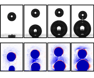
3.4. Schlieren images of scenarios I–III
To provide evidence on the potential mechanisms underlying scenarios I–III, we analyse in figure 5 the vertical temperature gradient using schlieren imaging. As shown in § 2, the term  $J_s/J_b - 1$, in which $J_s$ and $J_b$ refer to the recorded intensities of the schlieren images with and without bubbles, is proportional to $\partial T/\partial z$; cf. (2.4). If $J_s/J_b-1 > 0$, then the temperature gradient in the vertical direction (from bottom to top) is positive; it is negative for $J_s/J_b-1 < 0$. Thus the red and blue colours in figure 5(a) denote an increase (red) or decrease (blue) in the temperature in the vertical direction (from bottom to top). Although the extent and instant of their appearance differ, figure 5(a) demonstrates the existence of blue regions on top of both bubbles for all three scenarios. This is reminiscent of the thermal boundary layer produced during bubble nucleation at the electrode on top of each bubble due to Joule heating. These boundary layers are advected during the rise of the first bubble and also during the growth of the second bubble. As a result, blue regions of decaying temperature are found near the top of the bubbles. It is also noticeable that the thermal schliere upstream of the second bubble rises faster due to the displaced electrolyte and the wake behind the first bubble. As soon as this schliere reaches the bottom of the first bubble, the deceleration of the latter sets in. For sufficiently small distances $H_{E2}$, belonging to scenario I, a denser schliere, i.e. a stronger gradient, is established close to the nadir of the first (top) bubble. This is illustrated in more detail by the horizontal profiles of $J_s/J_b-1$ shown in figure 5(b) for each scenario. These profiles were taken in the grey boxes between both bubbles, depicted in the first row in figure 5(a) and averaged over 10 pixels ( $17.4\,\mathrm {\mu }$m) in the vertical direction. The black, red and blue lines marked as 2, 3 and 4 correspond to the snapshots in columns 2–4 of figure 5(a). On comparing the three scenarios, it becomes obvious that $J_s/J_b-1$ attains its highest (negative) magnitude for scenario I, and reduces constantly towards scenario III. Thus scenario I indeed possesses the highest temperature gradient in the vicinity to the bottom of the first bubble, i.e. from $-$100 to $100\,\mathrm {\mu }$m. As a result, a significant temperature gradient along the interface of the first bubble is created. The resulting shear stress (cf. § 4) is assumed to be responsible for its downward acceleration towards the second bubble. As a result of this reverse motion, the thermal boundary layer on top of the first bubble develops a characteristic shape resembling a flying bird. If the bubble is further away from the electrode (scenario II), then the schliere still touches the first bubble. However, the resulting temperature gradient is too weak to provoke an acceleration leading it to coalesce with the second bubble. In scenario III, the blue zone of elevated temperature is too far from the first bubble, hence there is no interaction at all.

Figure 5. (a) Schlieren images, represented by the dimensionless intensity  $J_s/J_b-1$, for different stages of scenarios I–III (1st–3rd row), shortly after $E_2=-8$ V is switched on, taken at $\Delta t= 3$ ms (1st row) and 4 ms (2nd and 3rd rows). (b) Profile of $J_s/J_b-1$ over the width of the image. Zero position – see the first image in (a) – corresponds to the electrode centre, which nearly coincides with the bubbles’ centres. The data were taken inside the grey boxes shown in (a). The black (2), red (3) and blue (4) lines correspond to the columns of the same number in (a), i.e. different instants of time. Panel (a) is supplemented by movies 5 to 7.
3.5. Multiple cycles
While previously only single cycles, as shown in figure 2, were studied, we analyse in figure 6(a) the position  $H$ of the first (red lines) and second (blue lines) bubbles during four cycles, C1–C4, of modulation of the potential (black line) within a single experimental run. The only difference to the foregoing experiments was that the second bubble during C1–C3 is produced in the same way as the first bubble, namely at $E_2=-6$ V for 1 ms. In the last cycle (C4), the potential $E_2$ was set to $-8$ V and applied continuously. Figure 6(b) documents snapshots of the bubbles’ behaviour for each cycle C1–C4 from figure 6(a), with the corresponding time stamps. Each cycle C1–C4 ends by coalescence. As a result, the coalescence radius of the first bubble increases from $R_1 = 70\,\mathrm {\mu }$m (C1) via $88\,\mathrm {\mu }$m (C2) and $100\,\mathrm {\mu }$m (C3) towards $110\,\mathrm {\mu }$m (C4). The important observation occurs when $E_2$ is set from $E_2 = -6$ V to $E_2 = 0$ to force the detachment of the second bubble. Despite the vanishing potential $E_2$, the first bubble thus still follows scenario I in a nearly unchanged way, i.e. it decelerates, moves towards the electrode, and finally coalesces with the second bubble.

Figure 6. Overview of the four bubble motion reversal cycles performed in succession. Each cycle, denoted by C1–C4, is marked by a different colour. (a) The variable  $H$ specifies the distance between the first bubble (red line) and the second bubble (blue line) and the electrode centre over time. The modulation of potential $E$ is shown by the black line. (b) Snapshots of the bubbles’ behaviour. The time stamps correspond to (a).
4. Discussion and conclusions
The key phenomenon discovered in this work is the contactless interaction between two hydrogen bubbles, produced by electrolysis. This interaction, which acts over distances equal to 5 times the diameter of the first bubble, is able to force a paradoxical reversal of the bubble motion in the direction opposite to buoyancy. The origin of this phenomenon needs to be sought in the forces  $F_e$ and $F_h$ (§ 1) acting on the bubble. However, an influence from the electric force $F_e$ can be excluded for two reasons:
(i) Bashkatov et al. (Reference Bashkatov, Hossain, Yang, Mutschke and Eckert2019) showed the nonlinear dependency of
$F_e$ and its strong decay for electrode distances larger than approximately $30\,\mathrm {\mu }$m. Thus the electric force is unlikely to play any role at the much larger bubble–electrode distances ${\approx }300\,\mathrm {\mu }$m found in this work.(ii) In figure 6, the first bubble was shown to follow scenario I in a nearly unchanged fashion, even when
$E_2$ is set to $E_2 = 0$, hence $F_e=0$.


This suggests that  $F_h$, and in particular the Marangoni force $F_M$, plays a key role. As revealed by the schlieren images in figure 5, the ${\rm H}_2$ bubble motion reversal in scenarios I and II sets in when the thermal boundary layer on top of the second bubble is able to touch the bottom of the first bubble. If this happens, then a temperature gradient is built up along the surface of the first bubbles. As the surface tension $\gamma$ decreases with increasing temperature, the gradient in surface tension pulls the adjacent electrolyte from the bubble foot towards the equator. As the $\gamma$ gradient mimics the action of the arms of a swimmer, the bubble starts moving opposite to the buoyancy force. This is in analogy to the classical work by Young et al. (Reference Young, Goldstein and Block1959) on thermocapillary migration. However, the big difference is that the temperature gradient has not been imposed externally but is generated in a self-organized way by the production of Joule heat and its dissipation by thermal diffusion. The resulting Marangoni force $F_M$ (see § 1 and below) for a spherical bubble in a homogeneous thermal gradient is given by (Morick & Woermann Reference Morick and Woermann1993):
 \begin{equation} F_{M} = 2{\rm \pi} R^2\left( -\frac{\partial \gamma}{\partial T}\,\frac{\partial T}{\partial z}\right). \end{equation}
Inserting (2.4) into (4.1), the Marangoni force  $F_M$, can be written as
 \begin{equation} F_{M} = 2{\rm \pi} R^2\left( -\frac{\partial \gamma}{\partial T}\right)k_1k_2 \left(\frac{J_s}{J_b}-1 \right)= k_3 \left(\frac{J_s}{J_b}-1 \right), \end{equation}
where  $k_3 = [ 2{\rm \pi} R^2(-({\partial \gamma }/{\partial T}))k_1k_2 ]$ is a positive constant for the present configuration. Thus if a bubble enters a region with a negative intensity ${J_s}/{J_b}-1<0$ (figure 5), then the Marangoni force will accelerate it downwards towards the second bubble. Figure 5(b) confirms this argument. It shows that the magnitude of ${J_s}/{J_b}-1$, and hence the Marangoni force, decreases from scenario I to scenario III. Moreover, a switch in the sign from ‘ $-$’ to ‘ $+$’ occurs in scenario III. Thus the Marangoni force is no longer directed downwards, and the phenomenon of attracting hydrogen bubbles (scenarios I and II) vanishes.
The stationary velocity of the ‘creeping’ thermocapillary migration of a bubble inside a temperature gradient  $\partial T/\partial z$ follows from Morick & Woermann (Reference Morick and Woermann1993) as
 \begin{equation} v = \frac{R^2 \rho g - \dfrac32\,R\left(\dfrac{\partial \gamma}{\partial T}\, \dfrac{\partial T}{\partial z}\right)}{3\mu}. \end{equation}
Taking the second peak velocity  $V_{p.2}\sim 30\,{\rm mm}\,{\rm s}^{-1}$ as the characteristic velocity $v$ of thermocapillary migration, the required $\partial T/\partial z$ according to (4.3) is approximately $90\,{\rm K}\,{\rm cm}^{-1}$. With the characteristic temperature rise $\Delta T \sim 10$ K at the microelectrodes (Massing et al. Reference Massing, Mutschke, Baczyzmalski, Hossain, Yang, Eckert and Cierpka2019; Hossain et al. Reference Hossain, Mutschke, Bashkatov and Eckert2020) over bubble radius $R \sim 100\,\mathrm {\mu }$m (0.01 cm), a much larger $\partial T/\partial z \sim 10^3\,{\rm K}\,{\rm cm}^{-1}$ can be achieved easily. This strongly supports the notion that (i) thermocapillary migration is at the origin of ${\rm H}_2$ bubble motion reversal, and (ii) the interaction of electrogenerated bubbles needs to be taken into account during water electrolysis.
Supplementary movies
Supplementary movies are available at https://doi.org/10.1017/jfm.2023.91
Acknowledgments
We thank J. Boenke for his support with experiments during his student internship in 2021.
Funding
This project is supported by the German Space Agency (DLR), with funds provided by the Federal Ministry of Economics and Technology (BMWi) due to an enactment of the German Bundestag under grant no. DLR 50WM2058 (project MADAGAS II), and the Hydrogen Lab of the School of Engineering of TU Dresden.
Declaration of interests
The authors report no conflict of interest.
Author contributions
A. Bashkatov identified the phenomena. A. Bashkatov and A. Babich conducted the experiments and contributed to this work equally. S.S.H., X.Y., G.M. and K.E. conceptualized the study. All authors contributed equally to analysing data and reaching conclusions, and to writing the paper.


 Open access