


1. Introduction
The theory of the nonlinear wave–wave interaction of gravity waves was presented first by Phillips (Reference Phillips1960). Since, a tremendous body of research has been conducted in this area. One of the biggest advances was by Benjamin & Feir (Reference Benjamin and Feir1967), who found that uniform Stokes waves in deep water are unstable to side band modulations. It was later termed the Benjamin–Feir instability (or modulation instability), which is a special case of four wave resonance. In fact, in much of the literature, the modulation instability is considered the cause of rogue waves, a current topic of interest. Unlike gravity waves, gravity–capillary waves can form three-wave resonances. The earliest work on resonant triads of gravity–capillary waves dates to McGoldrick (Reference McGoldrick1965) and Simmons (Reference Simmons1969). McGoldrick (Reference McGoldrick1970) conducted experiments on the resonant interaction of gravity–capillary waves, which provided their first experimental evidence. Subsequently, as an extension of modulation instability, McLean (Reference McLean1982) introduced a transverse instability which he termed type II. For a systematic review through the 1990s, see the review in Hammack & Henderson (Reference Hammack and Henderson1993). Recently, an unconventional new possibility of wave–wave interactions arose: resonance without energy exchange studied by Liao (Reference Liao2011). A steady-state resonance can also be found for pure capillary waves; see (Chabane & Choi Reference Chabane and Choi2019). Under appropriate circumstances, two-dimensional Stokes waves can bifurcate to three-dimensional waves. This was first studied by Saffman & Yuen (Reference Saffman and Yuen1980). Bifurcations can lead to two types of two-dimensional patterns: skew and symmetric. Su (Reference Su1982), and Su & Green (Reference Su and Green1984) experimentally verified and observed the bifurcations of gravity waves as both skew and symmetric patterns were observed.
When surface tension is considered, features of the water waves change. The rich effects that surface tension has on nonlinear waves have been studied widely. Several researchers (Meiron, Saffman & Yuen Reference Meiron, Saffman and Yuen1982; Chen & Saffman Reference Chen and Saffman1985; Zhang & Melville Reference Zhang and Melville1987) conducted numerical and analytical analyses of the three-dimensional bifurcation of gravity–capillary and pure capillary waves. These are extensions of the theory for gravity waves. The bifurcations are derivable from both Zakharov equations and Laplace equations with fully nonlinear boundary conditions; symmetric crest and symmetric troughs are realized. To the authors’ knowledge, no experimental work has demonstrated bifurcations for gravity–capillary waves. Several authors (Hammack, Scheffner & Segur Reference Hammack, Scheffner and Segur1989; Perlin, Henderson & Hammack Reference Perlin, Henderson and Hammack1990) experimentally investigated gravity–capillary waves. Using a wave-maker, they found experimental evidence of spectral spreading and resonant triads. In their experiments, elongated hexagons were found on the water surface, but no explanation was provided. Numerical analysis of three-dimensional gravity–capillary waves is also in the literature. Tsai & Hung (Reference Tsai and Hung2007) introduced surface tension in the fully nonlinear boundary conditions and simulated transverse instabilities of gravity–capillary waves. Although the theory of resonant triads for gravity–capillary waves was introduced decades ago, it seems not to have been measured accurately in two surface dimensions until Haudin et al. (Reference Haudin, Cazaubiel, Deike, Jamin, Falcon and Berhanu2016). Using a new surface measurement technology, Haudin was able to observe resonant triads of gravity–capillary waves with two-dimensional surface patterns. Cazaubiel et al. (Reference Cazaubiel, Haudin, Falcon and Berhanu2019) experimentally generated a forced resonant triad which contains waves that do not satisfy the dispersion relation. More recently, a free-surface synthetic Schlieren (FS-SS) method introduced by Moisy, Rabaud & Salsac (Reference Moisy, Rabaud and Salsac2009) was used to measure three-wave interactions (Abella & Soriano Reference Abella and Soriano2019). Transverse instability was observed also for gravity–capillary soliton waves (Park & Cho Reference Park and Cho2018). However, for most of the previous experiments, the results only show the spatial spectra and little information about the time evolution of the resonant triads was obtained.
On the other hand, cross-waves were first observed by Faraday in 1831. Lin & Howard (Reference Lin and Howard1960) investigated resonantly excited standing cross-waves in a rectangular tank. A theoretical analysis of cross-waves was presented by Garrett (Reference Garrett1970), who obtained a Mathieu equation indicating that the waves are caused by parametric resonance and subharmonic instability. Barnard, Mahony & Pritchard (Reference Barnard, Mahony and Pritchard1977) conducted an experimental study on the wave patterns generated by a torsional oscillating plate about a hinged vertical axis and they suggest that both nonlinearity and damping determined the wave pattern. The evolution equations for cross-waves were first derived by Jones (Reference Jones1984) using weakly nonlinear theory; it can be described in the form of a nonlinear Schrodinger equation (NLS). Since then, many experiments on cross-waves have been conducted. Lichter & Shemer (Reference Lichter and Shemer1986) did experiments in a long tank using a paddle-type wave-maker and found a strong modulation of cross-wave amplitudes as well as periodically generated solitons propagating from the wave-maker. Lichter & Chen (Reference Lichter and Chen1987) studied gravity cross-waves numerically and simulated a propagating staggered pattern under high forcing amplitudes. Using the same facility as Lichter & Shemer (Reference Lichter and Shemer1986), Shemer & Kit (Reference Shemer and Kit1989) observed four regimes of cross-wave patterns including steady, unsteady, modulational and chaotic. The modulated and chaotic cross-waves were further studied experimentally (Underhill, Lichter & Bernoff Reference Underhill, Lichter and Bernoff1991). Besides the longitudinal and subharmonic cross-waves, Tsai, Yue & Yip (Reference Tsai, Yue and Yip1990) found a chaotic motion that involved internal interactions between these two patterns. Very few experiments of capillary effects on cross-waves can be found in the literature. Recently, Moisy et al. (Reference Moisy, Michon, Rabaud and Sultan2012) investigated cross-waves in the gravity–capillary regime using a fully submerged, vertical wave-maker. They found a pattern that showed superposition of two oblique progressive waves. Like most cross-waves, this pattern only occurs in the vicinity of the wave-maker. Moisy suggested that it may be caused by three-wave interactions, but it was only a suggestion. Oblique subharmonic waves can also be generated in horizontally vibrated containers; Porter et al. (Reference Porter, Tinao, Laverón-Simavilla and Lopez2012) performed a series of experiments on cross-waves generated in a container subject to horizontal oscillations. Two oblique subharmonic waves were observed near the sidewalls, but similar to Moisy et al. (Reference Moisy, Michon, Rabaud and Sultan2012), the oblique cross-waves in these experiments only exhibit a few wavelengths in the longitudinal direction. The results are compared later to the theoretical predictions presented by Perez-Gracia et al. (Reference Perez-Gracia, Porter, Varas and Vega2014), the predicted oblique angles were generally consistent with the experiments. The boundary conditions on the sidewalls and on the wave-maker are important factors in forming cross-waves. Porter et al. (Reference Porter, Tinao, Laverón-Simavilla and Lopez2012) utilized a sharp edge along the top with a coated anti-wetting agent to pin the contact line, both pinned and dynamic contact line conditions were studied. A fixed contact line is preferred in modelling the pattern as a dynamic contact line introduces additional complexity. Rather than cross-waves generated by two-dimensional wave-makers, Shen & Liu (Reference Shen and Liu2019) studied theoretically the subharmonic resonant interaction of an axially symmetric wave, and found radially propagating cross-waves with decaying energy.
Another study shows a similar two-dimensional bi-periodic surface pattern; in the literature (Hammack & Henderson Reference Hammack and Henderson2003; Hammack, Henderson & Segur Reference Hammack, Henderson and Segur2005; Henderson, Segur & Carter Reference Henderson, Segur and Carter2010), a programmed wave-maker is used to generate a two-dimensional pattern of gravity–capillary waves. This can be interpreted as directly generating solutions of the NLS on the water surface. Steady two-dimensional surface patterns were realized. Although no evidence of bifurcation was seen, a persistent two-dimensional wave pattern was observed. Spatial wave spectra were also obtained; however, they were obtained by Fourier transform of the grey levels of images, not via surface elevations, and hence not as accurate. Fuhrman & Madsen (Reference Fuhrman and Madsen2006) provided a numerical simulation of the Hammack et al. experiments; the results exhibit similar features. Both the experimental and numerical results show stable wave patterns despite the fact that the solution of the two-dimensional NLS is proven to be unstable under three-dimensional perturbations. It was suggested by Segur et al. (Reference Segur, Henderson, Carter, Hammack, Li, Pheiff and Socha2005) that the presence of dissipation could stabilize the instability. Although these wave patterns are in the gravity regime and the generation mechanism is not subharmonic instability, they are worth mentioning because the wave patterns are quite similar to the experimental results shown in this study – a propagating steady wave pattern that contains two oblique wave components. The oblique cross-waves have been studied often, however, the underlying mechanism is far from fully understood. The spectra, the energy distribution and the time evolution of oblique cross-waves need to be further studied.
Both resonant triads and cross-waves will lead to nonlinear responses for steep gravity–capillary waves, and have been discussed theoretically and experimentally previously. In most of the previous research, the two nonlinear effects show particular wave patterns and were often studied separately. In this study, experimental results show similar patterns arise from these two different mechanisms, using the same wave-making method but with different levels of nonlinearity. Gravity–capillary multi-component wave patterns arise naturally by a planar wave-maker oscillated at a single frequency vertically or horizontally along one boundary of the basin. The temporal- and spatial-resolved surface profiles are measured using the FS-SS method. Exciting frequencies in this work are from 25 Hz through 40 Hz, within which capillary effects are significant. Surface tension is inferred via linear wave theory and is determined to be 70 mN m $^{-1}$. Multi-dimensional Fourier transforms are utilized to track the evolutionary spectra of the water surface in both time and space. Wavelet transforms are implemented to show times when various frequencies develop. Two kinds of multi-component wave patterns are realized, one from resonant triads and the other from oblique propagating cross-waves. The regimes of nonlinear wave patterns are delineated. The remainder of the paper is organized as follows. Section 2 introduces the experimental set-up; § 3 focuses on two types of resonant triads generated by horizontally oscillating the wave-maker. In § 4 trapped and propagating cross-wave results are presented. Both §§ 3 and 4 include comparisons between experimental and theoretical results. Some general concluding remarks are drawn in § 5.
2. Experimental set-up
The experiments are conducted in a glass wave tank 300 mm long and 151 mm wide. The water depth is 40 mm for each experiment. For the wave-maker frequencies used in this study (25 Hz through 40 Hz), all waves can be considered as deep-water waves. As pinned contact lines are desired, the sidewalls of the tank are coated with a hydrophobic material (Teflon). A 9 mm thick flat plate is placed at one end of the tank, with the plate attached to an electrodynamic shaker (Modal Shop, Model 2110E) that depending on orientation provides vertical or horizontal (sinusoidal) excitation here from 25 Hz through 40 Hz. A high-speed imager (Phantom VEO340L) operating at 500 frames per second with a 50 mm f/1.8D lens (Nikon AF Nikkor) is used to record the distortion to a random pattern positioned beneath the transparent tank bottom, which is used then to recreate the water surface (FS-SS). The high-speed imager is placed above the water tank. Figure 1 provides a schematic view of the facility. Figure 1(a) depicts the experimental configuration for the vertically oscillating wave-maker; figure 1(b) presents a sketch of the horizontally oscillating wave-maker, both the vertical and horizontal wave-makers have an adjustable immersion depth from 5 mm to 15 mm. The coordinate system used herein is shown in figure 1(c); the longitude direction of the wave tank is the  $x$-axis; the lateral direction is the $y$-axis. The displacement of the plate is measured using a linear variable differential transformer, linear position sensor with one end fixed and the other end attached to the wave-maker. The displacement data are acquired with a National Instruments cRIO-9067 system and LabView software. The procedure to obtain the free-surface measurements using the FS-SS technique is as follows: first, for calibration, one frame of the random pattern is recorded with a quiescent surface; for the experiments conducted, the calibration yields a horizontal resolution of 4.31 pixels mm $^{-1}$, which resolves the wavelength measurement to 0.23 mm, with corresponding uncertainty of 0.12 mm. For the 14.4 mm wave (16 Hz) in this study, this results in an accuracy of 0.8 %. Next, the frequency and peak-to-peak stroke are set for the shaker. The distorted random pattern that occurs due to the disturbed water surface is captured by the high-speed imager. A digital image correlation algorithm is used to calculate the displacement field of the random dot pattern. The original displacement is in pixels and is transformed to millimetres using the calibration result. Finally, based on the displacement field and the calibration result, FS-SS is used to reconstruct the free-surface elevation, $\eta$, for each frame recorded by the high-speed imager (see details in Moisy et al. Reference Moisy, Rabaud and Salsac2009). Thus, both temporal and spatial measurements of the water surface are obtained. The $x$ and $y$ direction accuracies (wavelength measurements) are well defined by the calibration results. To evaluate the $z$ direction accuracy (i.e. the surface elevation measurement), a plano-convex lens with known geometrical shape (Newport KPX184) is placed on the bottom of the tank above the random dot pattern to mimic the distorted water surface (as shown in figure 2); the refractive index of the lens is 1.51. The result of the FS-SS method in measuring the surface profile is also shown in figure 2. The FS-SS result shows very good agreement with the manufacturer provided profile of the lens.

Figure 1. Experiments set-up for FS-SS. (a) Vertically oscillating wave-maker, (b) horizontally oscillating wave-maker and (c) coordinate system used (planform view).

Figure 2. Surface profile of a plano-convex lens measured by FS-SS. (Upper left: three-dimensional reconstruction; upper right: image taken by high-speed imager; lower: comparison with manufacturer provided profile).
Near the wave-maker, the cross-waves are much steeper, and the FS-SS method has limited accuracy there. Laser induced fluorescence (LIF) is used to measure the transverse wave profile there. As shown in figure 3, a laser sheet is projected through the water surface that covers the entire lateral extent of the tank near the wave-maker. The amplitude of the cross-wave at the first crest is measured. Laser induced fluorescence is also a good method to verify or not the pinned contact line condition at the wall. Figure 4 shows the wave profile at different instants near the sidewalls with the white vertical lines added to the figures to depict the sidewall. In the lower row of images, the sidewalls are not treated with a hydrophobic coating and due to the smoothness of the sidewall, reflected wave images (although fainter) can be seen on the other side of the wall. The contact point is not fixed during the wave evolution. In the upper set of figures, the sidewalls are treated with the Teflon hydrophobic coating; it can be seen that the contact point is fixed. To better display the contact point, the vertical dimension of the picture is exaggerated by a factor of two. The elapsed time for each set of images is approximately one period of the primary frequency. In the unpinned case, due to the concave meniscus on the smooth wall, the surface level near the wall is higher than the mean water level. For the subsequent experiments herein, all the sidewalls are treated with a hydrophobic coating and can be considered to have a pinned contact line. This would be crucial in modelling the boundary conditions for the cross-waves.

Figure 3. Experimental set-up for LIF.

Figure 4. Five pinned (upper images) and unpinned (lower images) contact lines as a function of approximately one period of the wave-maker frequency. White horizontal lines: contact point level at  $t=0$; red lines: mean water levels throughout the experiments. The field of view is 35 mm in the $y$ direction and 17.5 mm in the $z$ direction.
In each experiment, five parameters are controlled: excitation frequency, tank width, wave-maker type (horizontally or vertically oscillated), peak-to-peak stroke and immersion depth. Deionized water is used in the experiments, and surface tension is inferred using linear wave theory. That is, the wavelength is measured at the different frequencies, and the data are least squares fit using the linear dispersion relation. First, a planar plunger type wave-maker is used to generate linear propagating waves. Then, the wave profile (including the measured wavelength) is determined using the FS-SS method. Based on the linear assumption, surface tension is obtained by substitution of the frequency and wavelength into the following linear dispersion relation:
 \begin{equation} \omega^{2}=gk+\frac{Tk^{3}}{\rho}.\end{equation}
Here  $\omega$ is the angular frequency of the waves, $g$ is the gravitational acceleration (9.81 m s $^{-2}$), $k$ is the wavenumber, $T$ is the surface tension and $\rho$ is the mass density of the deionized water (1000 kg m $^{-3}$). Two types of wave-makers are used in this study: one wave-maker is a piston type and moves horizontally, the other is a flat plate that is oscillated vertically. Both of them have a plate thickness of 9 mm and span the tank laterally. The horizontal wave-maker is used in generating resonant triads (with or without first subharmonics). The vertical wave-maker is used to generate cross-waves. The reason for selecting a vertical oscillating wave-maker is that it minimizes the amplitude of the primary plane waves; this is favourable when there is interest in cross-waves rather than resonant triads. By increasing the stroke of the wave-maker, of course, the system becomes more nonlinear, and the wave pattern evolves. Experiments performed in this study are summarized in table 1. Table 1 is sorted by excitation frequency. The wave pattern obtained in each case is listed in the last column where CW represents cross-waves and RT represents resonant triads. The cases with asterisks represent resonant trials with its first subharmonics; this will be discussed in § 3.2. Several non-dimensional numbers are used to compare the experimental results under different forcing parameters; the detailed analyses are discussed in the following sections.
Table 1. Parameters for the experiments. In the wave pattern column, CW represents cross-waves and RT represents resonant triads (*: resonant triads with subharmonics).

3. Three-wave interactions
In gravity–capillary waves when wave vectors  $\boldsymbol {k}$ and frequencies $\omega$ satisfy the kinematical condition,
 \begin{equation} \boldsymbol{k_1} \pm \boldsymbol{k_2} \pm \boldsymbol{k_3}=0; \quad \omega_1\pm \omega_2\pm \omega_3=0, \end{equation}
a resonant triad is formed; the system then yields a set of nonlinear coupled equations for the evolution of the amplitude for each triad member. Consider a two-dimensional water surface; there are many possibilities of resonant triads for each excitation frequency. In a particular (degenerate) two-dimensional surface case, if
 \begin{equation} \omega_1= \omega_2= \frac{\omega_3}{2}\end{equation}
then the two first subharmonics and the primary wave form a resonant triad. In a one-dimensional surface these collinear waves can form Wilton ripples at specified frequencies (e.g. 9.8 Hz for the first Wilton ripple). For two-dimensional surfaces, the subharmonics will be symmetric in wavenumber space, and experimental results in the next subsections show that these subharmonic wave vectors will form a regular two-dimensional surface pattern. In this section two different types of resonant triads are generated by a horizontally oscillating wave-maker, one without first subharmonics and one with first subharmonics.
3.1. Resonant triads without first subharmonics
As shown in figure 1(b), a wall is placed close to the wave-maker, and the waves then reflect and steepen; without the wall, the waves dissipate more rapidly, and the nonlinear phenomenon is not as easily observed. The distance between the wave-maker and the downstream wall is 100 mm. The stroke of the wave-maker in this case (horizontally) is 0.5 mm. There are necessarily gaps between the wave-maker and the sidewalls (0.5 mm) that act as two point sources. Due to these corner effects, a radial spread of wavenumber vectors is generated (can be seen from the spectra in figure 5), which provides fruitful wave components/perturbations that initiate resonant triads.

Figure 5. Wave pattern and spectra of a resonant triad without first subharmonics, generated by the horizontally oscillating wave-maker at 32 Hz and peak-to peak stroke of 0.5 mm (case 12): (a,d)  $t=5$ s; (b,e) $t=10$ s; (c,f) $t=15$ s. (a,b,c) Reconstructed surfaces; (d,e,f) spatial spectra.
Resonant triads are observed in our experiments under many excitation frequencies, and these are demonstrated for a 32 Hz excitation; the phenomenon for other frequencies is similar. As the stroke of the wave-maker is increased, the waves become sufficiently steep to form a resonant triad. Figure 5 shows three different stages of the resonant triad. In the upper insets (a–c) are the reconstructed surface profiles, while in the lower figures (d–f) are their corresponding spatial spectra, the domain of computation is  $100\ \textrm {mm} \times 150\ \textrm {mm}$. Initially with very small nonlinearity, the primary plane wave component is dominant, along with small circular components due to the corner effects. As nonlinearity/stroke is increased, the resonance becomes visible as the other two components required in the triad are amplified (see figure 5b,e). The energy is not all concentrated in these frequencies and some adjacent frequencies can still be measured, thus, the surface seems irregular (as can be seen in figure 5b). The third stage shown in (c) and (f) exhibits a more regular pattern, where four oblique components dominate the surface. The wave height and wavelength of each crest in the surface pattern shown in figure 5(c) is measured and the mean steepness ( $ka$) of the surface at this instant is determined to be 0.17. Rather than the two oblique components required to complete a resonant triad, the spectra show four components due to the reflection from the sidewalls, these provide another two symmetric components; thus, this also is a standing resonant triad. The surface pattern is more ‘regular’ in the third stage; after, the energy transfer back to the primary waves makes the surface irregular again. Figure 6 shows the evolutionary spatial spectra of this process, the time interval between each spectrum is five seconds. The wave pattern starts with primary waves at the excitation frequency; then angular spreading is observed. After about 10 s, the resonant triad starts to form; at about 15 s the energy of the primary waves reaches a minimum and the daughter waves obtain maximum energy. At this point, the waves form a regular two-dimensional pattern (figure 5c); as time continues, the energy of the primary waves starts to increase again, while the energy of the daughter waves starts to decrease. Although the primary waves decrease and increase alternately, due to dissipation, the system does not return exactly to the initial state. When the primary wave contains minimum energy, the wave pattern shows a regular shape, and the shape disappears as the primary waves regain most of their energy. Thus, the regular two-dimensional pattern disappears and reappears as the energy continues to shift among the three components.

Figure 6. Wavenumber spectra evolution of resonant triad without first subharmonics generated by the horizontally oscillating wave-maker at 32 Hz and peak-to peak stroke of 0.5 mm (case 12).
Figure 7 shows the spatial and temporal spectra of the resonant triad. Figure 7(a) shows the spatial spectra of the water surface during the third stage where the wavenumber vectors satisfy the resonance conditions, (3.1a,b). Figure 7(b) is the time series measured at one random point on the surface, and figure 7(c) is its Fourier point spectrum. Here, the spectrum is obtained using a 20 s time series, hence, the frequency resolution is 0.05 Hz, and the corresponding uncertainty is  $\pm$0.025 Hz. This accuracy holds for all the Fourier transforms in the later analyses. Three frequency components, $f_1=12.0$ Hz, $f_2=20.0$ Hz and $f_3=32$ Hz are observed; the amplitude of wavenumber vectors measured are $|k_1|=318$ m $^{-1}$, $|k_2|=511$ m $^{-1}$ and $|k_3|=760$ m $^{-1}$, respectively, while the angle between $k_1$ and $k_3$ is $28^{\circ }$, and the angle between $k_2$ and $k_3$ is $17^{\circ }$. All the components of the triad satisfy the dispersion relation. Hence, the waves meet the resonance conditions. It is also worth noting that the $y$-components of the oblique waves fit the width of the tank; this indicates that the width of the tank $b$ is an integer times the half $y$-component wavelength $\lambda _y$. In this case, the two oblique components have the same measured $\lambda _y= 42.0$ mm, thus $b/\lambda _y\approx 3.5$. This is not surprising since the system needs to satisfy the pinned contact line condition on the sidewalls. There may be other solutions that also satisfy both the resonant triad condition and the boundary conditions; the reason the system selects 12 Hz and 20 Hz is not yet clear. Additional work is needed to understand the selection of daughter frequencies in the resonant triads without subharmonics. The resonance condition for the $y$-components will be discussed in detail in § 4. Both figures 7(a) and 7(c) only show global spectra (spectral information for the entire space or the entire duration) of the surface elevation. However, it is instructive to study how the spectra evolve in time. The time-frequency analysis of the surface elevation is performed via a wavelet transform. Unlike the traditional Fourier transform, the wavelet transform employs so-called wavelets, rather than sinusoidal functions, as the transform basis functions. It adds a scale variable in addition to the time variable in the inner product transform. Hence, it is effective for time-frequency localization. In other words, it is able to capture the variation of spectra in time. In this study, the Morlet wavelet is used in decomposition of the time series, and the wavelet spectra is shown in figure 7(d). It can be seen that initially only the primary wave component exists. At approximately 10 s, two other frequency components are recognizable, and form a resonant triad. The amplitude of the primary component decays, while the amplitude of the two oblique components grows. This is typical of energy transfer among a resonant triad.

Figure 7. Time-frequency analysis of a  $f$ resonant triad without first subharmonics generated by the horizontally oscillating wave-maker at 32 Hz and peak-to peak stroke of 0.5 mm (case 12). (a) Spatial spectrum at $t=16$ s, (b) time series, (c) Fourier spectrum, (d) wavelet transform.
3.2. Resonant triad with first subharmonics
When the peak-to-peak stroke increases from the previous state to 0.9 mm (case 13), the previous triad no longer occurs, rather the first subharmonics (waves with half the excitation frequency) are generated. The two symmetric subharmonics and the primary plane wave form a different set of resonant triads. Now, this satisfies the resonance conditions, (3.1a,b) and (3.2). The surface reconstruction and two-dimensional spatial spectrum can be seen in figure 8. In this case, two side band waves are of the same frequency, the energy transfers from the primary wave to the two subharmonics. Here,  $f_1=f_2=16$ Hz, $f_3=32$ Hz and the amplitudes of wavenumbers measured are $|k_1 |=|k_2 |=432$ m $^{-1}$ and $|k_3|=763$ m $^{-1}$, respectively. The angle between $k_1$ and $k_3$, the angle between $k_2$ and $k_3$, both are $27^{\circ }$. As such, the waves meet the resonance conditions. When the three-wave components have roughly the same amplitude, the water surface looks irregular; see figure 8(a). Later, as shown in figure 8(b), the two symmetric subharmonics dominate the water surface, and a regular two-dimensional wave pattern is formed; the pattern resembles a series of elongated hexagons (also see photographs in figure 9). Although the pattern visually resembles hexagons, it is actually rectangular based on the information in the spectra. Using the same method as in the previous section, the mean steepness ( $ka$) of the surface shown in figure 8(b) is determined to be 0.24. The energy transfer is not limited to one direction: the regular two-dimensional pattern occurs, disappears and reappears as the energy continues to shift among the three components. Figure 10 is the spatial and temporal spectra of the resonant triad with subharmonics; the format of the figure is similar to figure 7. From figure 10(c), it can be seen that the two daughter waves (16 Hz) are the exact first subharmonics of the excitation frequency (32 Hz). From the wavelet spectrum 10(d), it can be seen that the resonant triad develops at about $t=13$ s, the energy of the primary waves decay while the energy of the subharmonics increase.

Figure 8. Reconstructed surface and wavenumber spectra of the resonant triad with its first subharmonics generated by the horizontally oscillating wave-maker at 32 Hz with peak-to-peak stroke of 0.9 mm (case 13): (a,b)  $t=12$ s, (c,d) $t=20$ s.

Figure 9. Images of wave patterns on the water surface formed by the resonant triad with its first subharmonics, same experiment conditions as in figure 8. (a) Before regular two-dimensional pattern forms,  $t=12$ s and (b) after regular two-dimensional pattern forms, $t=20$ s.

Figure 10. Time-frequency analysis of a resonant triad with first subharmonics generated by the horizontally oscillating wave-maker at 32 Hz with peak-to-peak stroke of 0.9 mm (case 13). (a) Spatial spectra at  $t=12$ s, (b) time series, (c) Fourier spectra, (d) wavelet transform.
4. Oblique propagating cross-waves
4.1. Subharmonic instability
According to Garrett (Reference Garrett1970), Ibrahim (Reference Ibrahim2015), the one-dimensional fluid free surface under an oscillating boundary condition may be described by Mathieu's equation in the form
 \begin{equation} \ddot{\eta}+4\nu k^{2}\dot{\eta}+(\omega_n^{2}-\hat{a}k\cos{\varOmega t})\eta=0,\end{equation}
where  $\omega _n$ is the natural frequency of the $n$th mode of the tank, $\varOmega$ is the wave-maker frequency, $k$ is the wavenumber and $\hat {a}$ is the acceleration of the excitation. The regime of instability is determined from
 \begin{equation} 1-\sqrt{\left(\frac{2\hat{a}k}{\varOmega^{2}}\right)^{2}-4\left(\frac{4\nu k^{2}}{\varOmega}\right)^{2}}\left(\frac{2\omega_n}{\varOmega}\right)^{2}<1+ \sqrt{\left(\frac{2\hat{a}k}{\varOmega^{2}}\right)^{2}-4\left(\frac{4\nu k^{2}}{\varOmega}\right)^{2}}, \end{equation}
which shows that the system is unstable to its first subharmonic. When the wave-maker peak-to-peak stroke gets sufficiently large, the system develops a subharmonic instability. As mentioned previously, the waves with primary frequency are spatially spread for all directions, and the subharmonic waves occur for all directions too. At the early stage of the wave evolution, all spread directions have a similar energy level; however, as the instability grows, the energy is concentrated on two transverse components, and cross-waves occur. In our experiments, depending on the resonance condition, the cross-waves will either be trapped or rotate through a slight angle and propagate downstream.
4.2. Trapped and oblique propagating cross-waves
The experiments in this study show that gravity–capillary cross-waves are trapped when the subharmonic frequency wavelength satisfies a natural mode of the tank. In other words, when the following equation is satisfied,
 \begin{equation} \frac{n}{2}\lambda=b, \quad n=1,2,3\ldots,\end{equation}
where  $n$ is the mode of the cross-waves, $\lambda$ is the wavelength of the subharmonic waves, and $b$ is the width of the wave basin. If this is the case, standing waves are observed adjacent to the wave-maker; these waves only exist near the wave-maker and the energy is trapped. The more frequent cases are when the resonance condition (4.3) is not satisfied; in other words, the subharmonic frequency is not in resonance with the natural sloshing modes. In these cases, an $x$-component is generated, and then the cross-waves become oblique to the end wall; this is a propagating subharmonic wave pattern. The free surface shows a two-dimensional, short-crested pattern as is evident from the photographs in figure 13. The oblique cross-waves were also reported in the literature. In Moisy et al.'s (Reference Moisy, Michon, Rabaud and Sultan2012) experiments the oblique waves only occur near the wall/wave-maker and only propagate a few wavelengths; hence, patterns similar to this study were not observed far downstream. The cross-waves dissipated rapidly in their experiments due to very low amplitudes. In Porter et al.'s (Reference Porter, Tinao, Laverón-Simavilla and Lopez2012) experiments a similar wave pattern was generated using a different method: horizontally oscillating the entire tank. Later, motivated by these experiments, Porter et al. (Reference Porter, Tinao, Laverón-Simavilla and Rodríguez2013) investigated the oblique cross-wave patterns theoretically, assuming localized parametric forcing. Slowly modulated (periodic) cross-waves were also observed experimentally; see (Tinao et al. Reference Tinao, Porter, Laverón-Simavilla and Fernández2014).
Figure 11 shows the reconstructed surfaces of oblique propagating cross-waves for two different frequencies, as well as their wavenumber spectra, the domain of computation is  $250\ \textrm {mm} \times 150\ \textrm {mm}$. Here the wave-maker oscillates vertically and the stroke of the wave-maker is 1.1 mm (case 5 and case 15). As can be seen in the figures, primary plane waves are present as well as oblique propagating cross-waves. This is more obvious in the 26 Hz excitation case. For higher frequencies, the plane waves are not obvious in the wave surface plots, but the components are still apparent in the spatial spectrum. It can be seen from the figure that the wave decays along the tank. The initial steepness ( $ka$) here is defined as the mean steepness of the first sets of crests adjacent to the wave-maker; they are 0.27 for 26 Hz excitations and 0.30 for 32 Hz excitations, respectively. Two symmetric oblique wavenumber vectors can be found in the wavenumber spectra, and the free surface can be written as
 \begin{equation} \eta(x,y,t)=a\cos{(k_xx+k_yy-\omega t)}+a\cos{(k_xx-k_yy-\omega t)},\end{equation}
where  $k_x$ and $k_y$ are the two components of the oblique cross-waves, and $a$ is their amplitude. The relationship between the wavenumber vectors in the oblique propagating cross-waves surface pattern is illustrated in figure 12. The parameters in figure 12 are defined as $k_p$: primary plane waves; $k_+, k_-$: oblique subharmonics; $k_x, k_y$: $x$ and $y$ components of the cross-waves; $\theta$: angle of the oblique waves, $\theta = arctan(k_y/k_x)$.

Figure 11. Water surface reconstructions and wavenumber spectra of oblique propagating cross-waves generated by the vertically oscillating wave-maker at 26 Hz (case 5) and 32 Hz (case 15) with peak-to-peak stroke of 1.1 mm.

Figure 12. Wavenumbers of oblique propagating cross-waves.
The phase speed in the  $x$-direction of the cross-waves can be calculated from
 \begin{equation} C_{px}=\frac{\omega_s}{k_x},\end{equation}
where  $\omega _s$ is the angular frequency of the subharmonic waves. As the magnitude of $k_x$ is much smaller than the magnitude of the oblique wavenumber vector $\boldsymbol {k}$ ( $k_x^{2}+k_y^{2}=|k|^{2}$), the $x$-direction phase speed of the cross-waves is much larger than the phase speed of the primary waves for this frequency, which according to linear theory is $C_p = \omega _s/k$. This is consistent with the experimental observations (see table 2). Table 2 provides a comparison of the measured and predicted parameters; the predicted values are all based on linear theory. Here, the wavenumber is predicted using the dispersion relation based on the subharmonic frequencies. It is also worth noting that the energy propagation speed for the oblique propagating cross-waves is much slower than the phase speed.
Table 2. Comparison of measured (obs) and predicted (pred) parameters under different excitation frequencies.

Based on the observations in our experiments in the gravity–capillary regime, when the resonance condition (4.3) is satisfied, once the gravity–capillary cross-waves are generated, they are trapped near the wave-maker. This phenomenon is consistent with the cross-wave theories for gravity waves. However, when the resonance condition (4.3) is not satisfied, oblique subharmonic waves are generated. In the latter case, the waves can be considered as a combination of two orthogonal components in  $x$ and $y$. Based on the experiments, the selection of the angle is dependent on both frequency and tank width. As discussed in § 2, the contact lines on the sidewalls are pinned, thus, in order to meet the boundary condition, the $y$-component must satisfy
 \begin{equation} \frac{n}{2}\lambda_y=b, \quad n=1,2,3\ldots,\end{equation}
where  $n$ is the mode of the cross-waves and $\lambda _y$ is the wavelength of the $y$-component. Theoretically, each $\lambda _y$ meeting the above condition is a practical solution; however, by repeating experiments for the same conditions, it is found that only one particular pattern is selected. How is the angle of the oblique waves selected? What parameters control the water surface pattern? To answer these questions, Moisy et al. (Reference Moisy, Michon, Rabaud and Sultan2012) suggested that the oblique subharmonic waves arise from a three-wave resonance with a characteristic length of the wave-maker, but Moisy did not provide verification. To verify this assumption, two different wave-makers with different plate widths are utilized (one 9 mm and the other 18 mm). Results show that there is no significant difference in terms of the angles of the oblique subharmonic waves, which indicates that, in this study, the width of the wave-maker is not the characteristic dimension that dictates a resonant triad. In addition, the wavenumber spectra shown in figure 11 do not indicate the three-wave vectors satisfy the resonance condition (3.1a,b). The oblique propagating cross-wave pattern remains steady for a fairly long period of time (our experiments last for more than 90 s and the surface pattern still persists) and the spectra do not evolve. This is similar to the steady two-dimensional pattern described by Hammack et al. (Reference Hammack, Henderson and Segur2005).
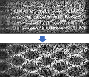
Figure 13 shows one frame of the recorded water surface using the high-speed imager. The upper part shows oblique propagating cross-waves with a regular two-dimensional pattern; the lower portion of the image shows typical cross-waves that are trapped near the wave-maker. In the upper portion of the figure the waves show clear travelling features while the lower one shows pure standing cross-waves. The energy of the standing cross-waves also travels downstream, but as one can see, the water surface is not steady or regular far downstream; it is different. In the upper image the whole wave pattern travels downstream. The two patterns are excited under the same stroke and frequency of wave-maker and in the same depth of water. The only difference is the tank width and, thus, as stated, the width of the tank plays an important role in pattern selection of the water surface. Due to the obliqueness, there are multiple wave modes that can satisfy (4.6) and the dispersion relation simultaneously. From the experiments performed, it is found that the system selects the mode with the minimum turning angle from the wall. In other words, the system selects the largest y-component wavenumber  $k_y$ that satisfies (4.6) and the dispersion relation, which will lead to a maximum $n$ (highest cross-wave mode). Select a 32 Hz excitation in a 151 mm wide tank, as an example. The oblique cross-wave frequency is 16 Hz, based on the dispersion relation, the wavelength of the oblique waves is $\lambda =14.5$ mm, and the wavenumber $k=436.6$ m $^{-1}$. To satisfy (4.6), the max $n$ available is 20, which leads to $\lambda _y=15.1$cm, $k_y=415.8$ m $^{-1}$, and the corresponding angle is $arctan(k_y/k_x)=73.75^{\circ }$. The mechanism selecting the angle of the oblique cross-waves is as follows: when the resonance condition (4.3) is satisfied, the cross-wave is perpendicular to the wave-maker, the angle is 90 degrees, and the wave pattern is trapped. When (4.3) is not satisfied, oblique cross-waves are generated, and the oblique wave needs to satisfy (4.6) as well as the dispersion relation. Among possible solutions, the system then selects the mode with the minimum turning angle from the wall. Based on these results, the process of generating the oblique waves can be described as follows: first, the wave-maker generates widespread directions of waves with the excitation frequency. Second, the system is unstable to its first subharmonic, and as the nonlinearity is increased, widespread directions of subharmonic waves are generated. Finally, the $y$-components of some subharmonic waves are in resonance with the natural frequency of the tank. Two symmetric, subharmonic waves with maximum mode, $n$, are amplified. They then dominate the wave field.

Figure 13. Planform view of the water surface of trapped (lower) and propagating (upper) cross-waves generated by the vertically oscillating wave-maker at 32 Hz, with peak-to-peak stroke of 1.1 mm, lower width: 72 mm (case 16), upper width: 61 mm (case 17).
The spectral evolution during the development of an oblique propagating cross-wave pattern is presented in figure 14. Four spectra present four different stages of the water surface. The time increment between insets from left to right is 6 s. As can be seen from the figures, the primary plane wave is generated first with a small amplitude followed by spread directional waves. Next, two selected oblique subharmonic waves are amplified. In the last stage two oblique propagating cross-waves dominate the energy spectrum. It needs to be pointed out that both types of wave-makers (horizontal and vertical) can generate oblique propagating cross-waves; the difference is the magnitude of the plane waves that share the same frequency with the wave-maker oscillation.

Figure 14. Wavenumber spectra evolution of oblique propagating cross-waves for 32 Hz vertically oscillating wave-maker with peak-to-peak stroke 1.1 mm (case 15). A six-second time increment is used between these spectra.
Using the above assumption, a series of predicted oblique wave angles to the wave-maker are calculated. These predicted angles are compared then with the measured angles in the physical experiments. The results are shown in figure 15 where the experimental results match quite well with the predicted ones. In the experiments a wall is added to change the width of the tank (as shown in figure 13); the wall is movable to obtain different widths. As there is no clear trend for the angle vs frequency or width, the comparison between the measured and predicted angles does not show a monotonic pattern. Multiple excitation frequencies and tank widths are used in the experiments. A non-dimensional number  $2b/\lambda$ is used to show the mode number of each angle, where $b$ is the width of the tank and $\lambda$ is the wavelength of the first subharmonics obtained by the dispersion relation. It can also be seen from figure 15 that the angle increases when the waves jump from a lower mode to the adjacent higher mode and decrease during the same mode as $2b/\lambda$ increases. This is consistent with the theoretical predictions. As expected, the mode number increases monotonically with the width under the same excitation frequency. The measured and predicted dispersion relation is shown in figure 16. It can be concluded that the subharmonics follow well the linear dispersion relation. Thus, these are free waves propagating from the wave-maker downstream. Although there is nonlinear distortion to the dispersion, the effect is minor. For example, take the 16 Hz subharmonic waves. According to linear dispersion (2.1), the wavelength is 14.4 mm. Considering nonlinearity, the dispersion relation for gravity–capillary waves in deep water is estimated to be
 \begin{equation} \omega^{2}=gk[1+(ka)^{2}]+\frac{Tk^{3}}{\rho}\left[1+\left(\frac{ka}{4}\right)^{2}\right]^{-{1}/{4}}. \end{equation}
At the highest level of nonlinearity in this study ( $ka=0.3$), the wavelength is calculated to be 14.6 mm. The difference, 0.2 mm, is within the resolution of the measurement and it decreases to 0.1 mm at $ka=0.2$. As the steepness drops dramatically away from the wave-maker, and the wavenumber is obtained from the entire surface, the nonlinear distortion to dispersion does not significantly affect the results.

Figure 15. Comparison of the measured and predicted angles of the oblique propagating cross-waves, excitation frequency from 28 Hz–34 Hz, tank width from 55 mm to 86 mm. The vertically oscillating wave-maker was used. Error bars are calculated from wavenumber measurements using standard error propagation techniques (cases 5, 10, 11, 16, 17, 23, 24, 25).

Figure 16. Comparison of measured and predicted dispersion, with error bars.
Similar to figure 7 in § 3, spatial and temporal spectra of the oblique subharmonic waves are shown in figure 17. Here, the excitation frequency is 26 Hz and the corresponding oblique subharmonic waves are 13 Hz. The wave-maker oscillation is initiated at  $t=0$ s. Figure 17(a) is the spatial spectrum of the free surface at $t=10$ s. It can be seen clearly that two oblique subharmonic waves are generated; the primary plane wave is very small but still is visible in the spectrum. In addition, small components of both the primary and subharmonic frequencies can be seen in nearly all directions. The corner effect of the wave-maker generates wavenumber vectors pointing in all directions and hence their subharmonics. Once the oblique propagating cross-waves develop, all other directions become very small, and only two selected components dominate. Figure 17(b) is the associated time series measured at one random point on the free surface; it shows that when subharmonic waves are generated, their amplitudes are much larger than the primary plane waves, indicating instability. Figure 17(c) is the Fourier spectrum for the time series where two frequencies are evident. Figure 17(d) shows the wavelet spectrum; it can be seen that the subharmonic waves occur at approximately $t=5$ s. The wave component with the excitation frequency (the primary plane wave) essentially maintains the same amount of energy throughout the experiment, as it is affected little by the generation of the subharmonic waves.

Figure 17. Time-frequency analysis of oblique propagating cross-waves generated by the vertically oscillating wave-maker at 26 Hz, with peak-to-peak stroke of 1.1 mm (case 5). (a) Spatial spectrum, (b) time series, (c) frequency spectrum, (d) wavelet transform.
4.3. Comparison of resonant triads and cross-waves
Two multi-component wave patterns of resonant triads and cross-waves are discussed in the previous sections. As mentioned earlier, the wave pattern is highly dependent on the stroke of the wave-maker, which is essentially the level of nonlinearity. It is found that the selection of the wave pattern also depends on the immersion depth of the wave-maker. In this section both resonant triads and cross-waves are generated using the same forcing type: horizontally oscillating the wave-maker. By changing the wave-maker stroke, the immersion depth and the excitation frequency, the wave pattern regimes are obtained, as shown in figure 18. Two non-dimensional numbers are used:  $\lambda /D$ and $ks$. Here $\lambda$ and $k$ are the wavelength and wavenumber of the primary waves, respectively; $D$ is the immersion depth and $s$ is the peak-to-peak stroke of the wave-maker. For all experiments discussed in this study, the excitation frequency varies from 24 Hz to 38 Hz, the peak-to-peak stroke of the wave-maker is varied from 0.3 mm to 1.5 mm, and the immersion depth is changed from 5 mm to 15 mm. Low $\lambda /D$ can be interpreted as an indication of parametric excitation (oscillating boundary) while $ks$ represents the level of nonlinearity.

Figure 18. Wave pattern regimes. Red  $x$'s are experiments that exhibit resonant triads; blue circles are experiments that exhibit cross-waves. The dashed line indicates the boundary between resonant triads and cross-waves. (All experiments are with a horizontally oscillated wave-maker; *: resonant triads with first subhamonics).
In figure 18 red  $x$'s represent experiments that exhibit resonant triads while blue circles are experiments with cross-waves. The black dashed line indicates the boundary between resonant triads and cross-waves. A horizontal boundary at lower $ks$ indicates that there is a critical $\lambda /D$ below which resonant triads are unlikely to form, which is around $\lambda /D=0.53$. It can be seen from the figure that under the same $\lambda /D$, as $ks$ increases, the pattern changes from resonant triads to cross-waves. Under the same $ks$, the cross-waves occur at lower $\lambda /D$, which means greater immersion depth (or lower excitation frequency) leads to cross-waves. Wave-makers with greater immersion depth act more like an oscillating boundary than those with a smaller immersion depth; the former ones introduce sufficient subharmonic instability and lead to cross-waves, while the latter ones fall into the resonant triad regime.
5. Discussion and concluding remarks
5.1. Steadiness of two-dimensional multi-component wave patterns
When two symmetric wavenumbers are formed, the water surface exhibits a regular two-dimensional pattern. This can be seen from the oblique propagating cross-waves and the resonant triads with subharmonics. Theoretically, superposition of two symmetric oblique waves forms a short crest rectangular pattern. In the oblique propagating cross-waves case the two oblique components are not affected by the primary plane waves; their energy is gained directly from the motion of the wave-maker (not from instability of the primary waves). The pattern is steady under a particular level of nonlinearity. The resonant triads, on the other hand, are a three-wave interaction where the three-wave components resonate and the two daughter waves gain energy from the primary wave; the energy continues to transfer among the components, the wave pattern evolves.
5.2. Development of nonlinearity
As observed from the experiments, there are three levels of nonlinearity that lead to three patterns of the water surface: selective triads without subharmonics, resonant triads with subharmonics and cross-waves. Figure 19 shows the wave components for different stages of nonlinearity. With an increase of wave-maker stroke, the amplitude of generated primary waves increases and quickly enters the nonlinear regime. When nonlinearity is small, resonant triads without first subharmonics are generated; at this point, subharmonic instability has yet to occur. The phenomenon of the energy transfer among the three wavenumbers is observed. As the stroke is increased further, the system enters another nonlinear regime where subharmonics are generated. Two oblique subharmonic waves and the primary plane wave form a different resonant triad. The development time of this triad is longer than the previous one and the wave surface forms a clear, regular two-dimensional pattern due to the symmetry of the wave vectors. The next phase of nonlinearity occurs when the stroke of the wave-maker is further increased, and subharmonic instability dominates the triads. In this phase, gravity–capillary cross-waves are generated. The pattern of the cross-waves (trapped or propagating) depends on the resonance condition. It is also worth noting that the transition from one stage to another is not direct. As the stroke is increased with resonant triads without subharmonics, the triad disappears quickly, the water surface returns to a plane-wave-only pattern, and then develops another resonant triad (with subharmonics). When the stroke is increased further from a resonant triad with subharmonics, the triad disappears and only primary plane waves are observed, followed by the new pattern: cross-waves. If the nonlinearity is increased further yet, the cross-waves will jump to another regime where modulation or even chaos can be observed.

Figure 19. Wave vectors at different levels of nonlinearity.
Supplementary movies
Supplementary movies are available at https://doi.org/10.1017/jfm.2021.754.
Declaration of interests
The authors report no conflict of interest.


 Open access