


1. Introduction
The evaporation of sessile droplets has received significant attention in recent years, being the subject of several major reviews (Cazabat & Guena Reference Cazabat and Guena2010; Lohse & Zhang Reference Lohse and Zhang2015; Brutin & Starov Reference Brutin and Starov2018; Wilson & D'Ambrosio Reference Wilson and D'Ambrosio2023) due to its ubiquity in theoretical, experimental and industrial settings. A particular phenomenon of interest is the so-called ‘coffee-ring effect’, in which a solute in such an evaporating droplet ends up preferentially accumulated at the contact line (Deegan et al. Reference Deegan, Bakajin, Dupont, Huber, Nagel and Witten1997, Reference Deegan, Bakajin, Dupont, Huber, Nagel and Witten2000). This effect is very robust, occurring even in situations where the solute is initially uniformly dispersed throughout the droplet, and where the evaporative flux is not preferentially localized at the contact line (Boulogne, Ingremeau & Stone Reference Boulogne, Ingremeau and Stone2016).
Motivated by typical physical parameters, models of such systems generally assume that the Péclet number is sufficiently large that diffusive effects can be neglected, and so the dynamics of the solute inside the droplet are governed purely by advection (Deegan et al. Reference Deegan, Bakajin, Dupont, Huber, Nagel and Witten1997; Wray et al. Reference Wray, Wray, Duffy and Wilson2021). This unphysical assumption leads to a variety of undesirable side effects, in particular, that the mass is swept into a ring of infinitesimal width at the contact line (Deegan et al. Reference Deegan, Bakajin, Dupont, Huber, Nagel and Witten2000).
A variety of attempts have been made to resolve this problem phenomenologically, including via the incorporation of jamming effects (Popov Reference Popov2005; Kaplan & Mahadevan Reference Kaplan and Mahadevan2015). However, jamming effects only become significant close to the particle packing fraction, and the assumptions underpinning the model fail long before this point. In particular, the assumption that diffusive effects can be ignored breaks down in a diffusive boundary layer close to the contact line (Moore, Vella & Oliver Reference Moore, Vella and Oliver2021), as might be anticipated from the singular accumulation in the naïve, advection-only model. This boundary layer and its growth and dynamics have been analysed and understood via matched asymptotics and careful numerics in situations where droplets are small and, thus, exist at quasi-static equilibrium due to surface tension (Moore et al. Reference Moore, Vella and Oliver2021; Moore, Vella & Oliver Reference Moore, Vella and Oliver2022), but little is known for larger droplets where the effects of gravity are important.
Investigations of larger droplets have a long history, dating back to numerical integration of the appropriate Laplace equations by Padday (Reference Padday1971) and Boucher & Evans (Reference Boucher and Evans1975), with a variety of studies via asymptotics of their shape (Rienstra Reference Rienstra1990; O'Brien Reference O'Brien1991; Allen Reference Allen2003) and stability (Pozrikidis Reference Pozrikidis2012) in the intervening time. The effect of gravity on droplets, and especially their internal flows, has experienced a recent resurgence of interest, primarily due to applications to droplets on an incline or in binary droplets of more complex fluids, such as printer inks or commercial alcohols. For droplets on an incline, gravity may break the symmetry of an evaporating sessile droplet by, for example, altering the evaporation rate (Timm et al. Reference Timm, Dehdashti, Jarrahi Darban and Masoud2019; Tredenick et al. Reference Tredenick, Forster, Pethiyagoda, van Leeuwen and McCue2021) or pinning time (Charitatos, Pham & Kumar Reference Charitatos, Pham and Kumar2021) compared with a sessile droplet on a flat substrate. These effects may also play a role in the coffee-ring phenomenon, leading to non-uniform ring-like stains (see, for example, Du & Deegan Reference Du and Deegan2015; Issakhani et al. Reference Issakhani, Jadidi, Farhadi and Bazargan2023), more complex patterns after droplet depinning (Charitatos et al. Reference Charitatos, Pham and Kumar2021), or in extreme cases where the droplet is pendant, the formation of a cone-like ‘coffee eye’ (Mondal et al. Reference Mondal, Semwal, Kumar, Thampi and Basavaraj2018). Meanwhile, the recent upsurge in interest in binary droplets has been driven by, for example, the experiments of Edwards et al. (Reference Edwards, Atkinson, Cheung, Liang, Fairhurst and Ouali2018), which showed that the dynamics of binary droplets can be sensitively dependent on both the component liquids (as well as droplet inclination), and hence, gravity. This has since received extensive investigation both experimentally and numerically (Pradhan & Panigrahi Reference Pradhan and Panigrahi2017; Li et al. Reference Li, Diddens, Lv, Wijshoff, Versluis and Lohse2019).
For sessile droplets, however, it is notable that, despite the original experiments of Deegan et al. (Reference Deegan, Bakajin, Dupont, Huber, Nagel and Witten1997) involving large droplets, there have been relatively few investigations of particle transport inside them, with those available being principally experimental (Sandu & Fleaca Reference Sandu and Fleaca2011; Hampton et al. Reference Hampton, Nguyen, Nguyen, Xu, Huang and Rudolph2012; Devlin, Loehr & Harris Reference Devlin, Loehr and Harris2016). This is perhaps because of the robustness of the coffee-stain effect: asymptotic and numerical investigations (Barash et al. Reference Barash, Bigioni, Vinokur and Shchur2009; Kolegov & Lobanov Reference Kolegov and Lobanov2014) confirm the experimental results that the ring stain is preserved unless additional physics is incorporated, such as continuous particle deposition (Devlin et al. Reference Devlin, Loehr and Harris2016). However, this neglects much of the transient dynamics of evaporation-driven solute transport, including the dynamics of the residue over the course of the lifetime of the droplets: a critical omission in continuous particle deposition in particular.
In this analysis, we seek to rectify this deficiency and explore the role that gravity may play in solute transport in an evaporating sessile droplet. In particular, we seek to determine how gravitational influences change from moderate Bond number, where we anticipate an asymptotic structure akin to that of surface-tension-dominated droplets discussed extensively in Moore et al. (Reference Moore, Vella and Oliver2021, Reference Moore, Vella and Oliver2022), to large Bond numbers, where the localized interplay of the effects of surface tension and solutal diffusion at the pinned contact line lead to a change in the size of the nascent coffee ring. In the former case, we show that gravity acts to weaken the coffee-ring effect, leading to shallower, wider ring profiles, potentially lengthening the validity of the dilute regime before solute jamming takes place (Moore et al. Reference Moore, Vella and Oliver2021, Reference Moore, Vella and Oliver2022), while simultaneously promoting the importance of effects such as free surface capture (Kang et al. Reference Kang, Vandadi, Felske and Masoud2016), which may otherwise play a secondary role for thin droplets. For large Bond numbers, we demonstrate that the properties of the ring are governed by a completely different set of scalings, and we investigate the transition between the two regimes in detail. Moreover, in both regimes, we demonstrate that the solute transport dynamics is actually quite subtle and complex compared with the zero-gravity problem, including the possibility of a secondary peak in the solute mass, and so certainly merits a detailed investigation.
The structure of this paper is therefore as follows. In § 2, we describe the equations governing the fluid flow and solute transport for the problem of a thin droplet evaporating in a diffusion-dominated regime, in particular highlighting the effect of gravity in the model. We non-dimensionalize the model and introduce the three key dimensionless numbers in the model: the capillary, Bond and Péclet numbers. In § 3, we solve for the liquid flow in the limit in which the solute is dilute, so that the flow and solute transport problems decouple. We discuss pertinent features of the resulting fluid velocity and droplet shape, and, in particular, how these features vary with the Bond number. The bulk of the analysis in this paper concerns the influence of gravity on solute transport within the droplet, which we analyse in the physically relevant large-Péclet number limit in § 4. We find that there are two distinct regimes depending on the relative sizes of the Bond and Péclet numbers. In the first, where the Bond number is moderate, we extend the asymptotic analysis of Moore et al. (Reference Moore, Vella and Oliver2021) to include the effect of gravity in § 4.1. However, when the Bond number is also large, a more complex asymptotic analysis is necessary, which is presented in detail in § 4.2. In each asymptotic regime, we derive predictions for the distribution of the solute mass within the droplet. We compare these predictions to results from numerical simulations in § 5. In particular, we explore the effect of gravity on the classical coffee ring in each of the above regimes, while also highlighting the emergent phenomenon of a secondary peak in the solute distribution for a band of Bond numbers. Finally, in § 6, we summarize our findings and discuss implications to various applications, as well as avenues for future study.
2. Problem configuration
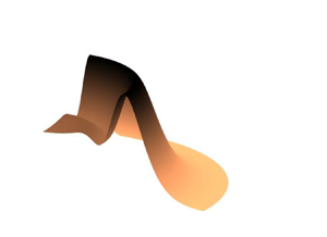
We consider the configuration depicted in figure 1, in which an axisymmetric droplet of initial volume  $V^{\ast}_{0}$ evaporates from a solid substrate. Here and hereafter, an asterisk denotes a dimensional variable. We let $(r^{\ast},\theta,z^{\ast})$ be cylindrical polar coordinates centred along the line of symmetry of the droplet with the substrate lying in the plane $z^{\ast} = 0$: by axisymmetry, we shall assume that all the variables are independent of $\theta$. The droplet contact line is thus circular and we assume that it is pinned throughout the drying process, which is observed in practice for a wide range of liquids for the majority of the drying time (Deegan et al. Reference Deegan, Bakajin, Dupont, Huber, Nagel and Witten1997; Hu & Larson Reference Hu and Larson2002; Kajiya, Kaneko & Doi Reference Kajiya, Kaneko and Doi2008; Howard et al. Reference Howard, Archer, Sibley, Southee and Wijayantha2023). We let $r^{\ast} = R^{\ast}$ be the radius of the contact line. Throughout this analysis, we shall assume that the droplet is thin, which reduces to the assumption that
 \begin{equation} 0<\delta = \frac{V^{\ast}_{0}}{R^{*3}} \ll1. \end{equation}
As we discuss presently, the thin-droplet assumption allows us to greatly simplify the flow and solute transport models; the assumption has been extensively validated and has shown to be reasonable even for droplets that should realistically fall outside of this regime (Larsson & Kumar Reference Larsson and Kumar2022).

Figure 1. A side-on view of a solute-laden droplet evaporating under an evaporative flux  $E^*(r^*)$ from a solid substrate that lies in the plane $z^* = 0$. The droplet is axisymmetric and the contact line is assumed to be pinned on the substrate at $r^* = R^*$. The droplet free surface is denoted by $h^*(r^*,t^*)$. The solute is assumed to be inert and sufficiently dilute that the flow of liquid in the droplet is decoupled from the solute transport.
The droplet consists of a liquid of constant density and viscosity denoted by  $\rho ^{\ast}$ and $\mu ^{\ast}$, respectively. The droplet free surface is denoted by $z^{\ast} = h(r^{\ast},t^{\ast})$ and the air–water surface tension coefficient, $\sigma ^*$, is assumed to be constant.
The liquid evaporates into the surrounding gas and we assume that the evaporative process is quasi-steady, which is a reasonable assumption for a wide range of liquid–substrate configurations (Hu & Larson Reference Hu and Larson2002). We denote the evaporative flux by  $E^*(r^*)$. The exact form of the flux will depend upon the dominant evaporative processes, which can change significantly with the properties of the droplet, ambient gas and substrate. Although it is not the goal of the present study to determine the correct form for $E^*(r^*)$, the differences do merit further discussion, which we pursue shortly in § 2.2.
The droplet contains an inert solute of initially uniform concentration  $\phi ^{\ast}_{0}$. The solute is assumed to be sufficiently dilute that the flow and transport problems completely decouple. We shall discuss the validity of the dilute assumption further in § 6.
2.1. Flow model
The droplet is assumed to be sufficiently thin and the evaporation-induced flow sufficiently slow that the flow is governed by the lubrication equations
 $$\begin{gather} \frac{\partial h^{\ast}}{\partial t^{\ast}} + \frac{1}{r^{\ast}}\frac{\partial}{\partial r^{\ast}}(r^{\ast} h^{\ast}u^{\ast}) =- \frac{E^{\ast}}{\rho^{\ast}}, \end{gather}$$
 $$\begin{gather}u^{\ast} =- \frac{h^{*2}}{3\mu^{\ast}}\frac{\partial p^{\ast}}{\partial r^{\ast}}, \end{gather}$$
 $$\begin{gather}p^{\ast} = p_{atm}^{\ast}-\rho^{\ast}g^{\ast}(z^{\ast}-h^{\ast}) - \sigma^{\ast}\frac{1}{r^{\ast}}\frac{\partial}{\partial r^{\ast}}\left(r^{\ast}\frac{\partial h^{\ast}}{\partial r^{\ast}}\right), \end{gather}$$
for  $0< r^{\ast}< R^{\ast}$, $t^{\ast}>0$, where $u^{\ast}(r^{\ast},t^{\ast})$ is the depth-averaged radial fluid velocity, $p^{\ast}(r^{\ast},z^{\ast},t^{\ast})$ is the liquid pressure and $p^{\ast}_{atm}$ denotes atmospheric pressure (Hocking Reference Hocking1983; Deegan et al. Reference Deegan, Bakajin, Dupont, Huber, Nagel and Witten2000; Oliver et al. Reference Oliver, Whiteley, Saxton, Vella, Zubkov and King2015).
We note here that we assume throughout the analysis that the lubrication equations (2.2)–(2.4) remain applicable in the regions of interest, most notably in the region close to the contact line where solutal diffusion becomes important. This will introduce restrictions on the size of  $\delta$ in cases where the effect of gravity dominates over surface tension, as we discuss in detail in § 3.
Equations (2.2)–(2.4) must be solved subject to the symmetry conditions
 \begin{equation} r^{\ast} h^{\ast}u^{\ast} = \frac{\partial h^{\ast}}{\partial r^{\ast}} = 0 \,\quad \text{at} \ r^{\ast} = 0, \end{equation}
and the fact that the free surface touches down at, and we require no-flux of liquid through, the pinned contact line, that is,
 \begin{equation} h^{\ast} = r^{\ast} h^{\ast}u^{\ast} = 0 \,\quad \text{at} \ r^{\ast} = R^{\ast}. \end{equation}
We close the problem by specifying the initial droplet profile, that is,
 \begin{equation} h^{\ast}(r^{\ast},0) = h^{\ast}_{0}(r^{\ast})\quad \text{for} \ 0< r^{\ast}< R^{\ast}. \end{equation}
 It is worth noting at this stage that, while this initial condition is needed to fully specify the mathematical problem, in our analysis we do not explicitly use (2.7). In what follows, it is assumed that the rate of evaporation is sufficiently slow that the droplet quickly relaxes under capillary action to the quasi-steady profile found in § 3 (see, for example, Lacey Reference Lacey1982; De Gennes Reference De Gennes1985; Oliver et al. Reference Oliver, Whiteley, Saxton, Vella, Zubkov and King2015). Thus, we shall, for simplicity, assume that  $h_{0}^*(r^*)$ is of the same functional form of the free surface we find in § 3. While this assumption is reasonable for a wide range of applications, for extremely rapid evaporation (for example, laser-induced evaporation, Volkov & Strizhak Reference Volkov and Strizhak2019), a more careful consideration of the evolution after deposition would be needed.
2.2. Evaporation model
As alluded to above, there are a number of different viable evaporation models depending on the physical and chemical characteristics of the problem (see, for example, Hu & Larson Reference Hu and Larson2002; Shahidzadeh-Bonn et al. Reference Shahidzadeh-Bonn, Rafai, Azouni and Bonn2006; Kelly-Zion et al. Reference Kelly-Zion, Pursell, Vaidya and Batra2011; Murisic & Kondic Reference Murisic and Kondic2011, and references therein). We shall outline a few of the more common cases.
A common evaporation model for small droplets (typically up to around a millimetre) with a pinned contact line is a diffusion-limited model, in which evaporation is limited by how quickly vapour is transported away from the droplet surface by diffusion and exhibits a singular flux at the contact line. Such a model has been shown to accurately predict both the total evaporation rate (Hu & Larson Reference Hu and Larson2002) and the pointwise evaporative flux (see, for example, Sáenz et al. Reference Sáenz, Wray, Che, Matar, Valluri, Kim and Sefiane2017; Wray & Moore Reference Wray and Moore2023) for a range of different droplet geometries.
When the ambient gas consists solely of vapour or when the diffusion of vapour is rapid, evaporation may instead be limited by kinetic effects at the liquid–vapour interface (see, for example, Murisic & Kondic Reference Murisic and Kondic2011; Jambon-Puillet et al. Reference Jambon-Puillet, Carrier, Shahidzadeh, Brutin, Eggers and Bonn2018). These effects are governed by the Hertz–Knudsen relation and may be shown for thin droplets to give an approximately constant evaporative flux. A constant flux may also be shown to be relevant in situations where a droplet evaporates above a hydrogel bath (Boulogne et al. Reference Boulogne, Ingremeau and Stone2016).
For larger droplets evaporating into a mixture of the liquid vapour and another gas, natural convection may be shown to play an important role in the evaporation rate for both pinned (Dollet & Boulogne Reference Dollet and Boulogne2017) and non-pinned (see, for example, Shahidzadeh-Bonn et al. Reference Shahidzadeh-Bonn, Rafai, Azouni and Bonn2006; Kelly-Zion et al. Reference Kelly-Zion, Pursell, Vaidya and Batra2011) droplets, although its role is greatly diminished when the density difference between the vapour and ambient gas is small (Radhakrishnan, Anand & Bakshi Reference Radhakrishnan, Anand and Bakshi2019). The relative importance of natural convection to vapour diffusion is measured by the Grashof number,
 \begin{equation} {Gr} = \left|\frac{(\rho_{s}^*-\rho_\infty^*)}{\rho_{\infty}^*}\right|\frac{g^*R^{*3}}{\nu_{air}^*}, \end{equation}
where  $\rho ^*_s$ is the vapour saturation density at the droplet free surface, $\rho ^*_\infty$ is the ambient vapour density and $\nu _{\text {air}}^*$ is the kinematic viscosity of air (Kelly-Zion et al. Reference Kelly-Zion, Pursell, Vaidya and Batra2011; Dollet & Boulogne Reference Dollet and Boulogne2017). When ${Gr}\ll 1$, diffusion dominates the evaporation, while for moderate and large ${Gr}$, convection effects are non-negligible and often dominant.
For the particular example of a large ( $R^* \geq 4$ mm) circular disk of water evaporating into ambient air, Dollet & Boulogne (Reference Dollet and Boulogne2017) show that the total evaporative flux $F^* = 2{\rm \pi} \int _{0}^{R^*} r^*E^*(r^*)\,dr^*$ may be approximated by the form
 \begin{equation} F^* \approx 2{\rm \pi} D^* R^* (c_s^*-c_\infty^*)\left[a_1{Gr}^{\beta} + a_2\right], \end{equation}
where  $D^{\ast}$ is the vapour diffusion coefficient, $c^*_s$ is the saturation concentration at the droplet free surface and $c^*_\infty$ is the ambient vapour concentration. The first term in the brackets corresponds to the importance of convection, while the second term is akin to the importance of diffusion. The exponent $\beta$ is estimated analytically to be $1/5$, which is shown to be very close to experimental data, where $\beta \approx 0.18$ with $a_1 \approx 0.31$ and $a_2\approx 0.48$. They show that for ${Gr}\approx 20$ – corresponding to a droplet radius of $R^*\approx 5$ mm – the contribution of convection is around $50\,\%$ larger than diffusion. The difference grows wider as $R^*$ is increased further. Kelly-Zion et al. (Reference Kelly-Zion, Pursell, Vaidya and Batra2011) find a similar scaling law, although with slightly different coefficients, for a range of different evaporating liquids.
Once convection is significant, it becomes prohibitively difficult to find explicit expressions of the evaporative flux valid for all  $r^*$. One can make scaling arguments based on boundary layer theory for large Grashof numbers, but these are unable to capture the flux near the droplet edge or at the centre of the droplet where a plume of vapour rises (Dollet & Boulogne Reference Dollet and Boulogne2017). Since these regions respectively play a crucial role in both the early time evolution of the coffee-ring (Moore et al. Reference Moore, Vella and Oliver2021, Reference Moore, Vella and Oliver2022) and the late time ‘fadeout’ profile of the ring (Witten Reference Witten2009), this severely hinders any prospect of analytic progress in studying solute transport in such regimes, and such approaches would necessarily be numerical.
It is not the goal of the present study to determine the correct model for evaporation for a given configuration and nor do we seek to cover the manifold possible models herein. Instead, our aim is to concentrate on the interplay between gravity, surface tension, solutal advection and solutal diffusion in solute transport, so here we shall choose an illustrative model for evaporation to use throughout the analysis, namely diffusive evaporation. Our choice is partly due to its predominance for smaller droplets (Hu & Larson Reference Hu and Larson2002) and for droplets evaporating in an ambient gas whose density is close to the vapour density (Radhakrishnan et al. Reference Radhakrishnan, Anand and Bakshi2019), but also due to access to an explicit form of the evaporative flux, as discussed shortly. While we recognize that there are regimes where this evaporation model will be lacking, the principles of the asymptotic analysis we pursue will be similar for a given flux – provided that we are in a regime where a coffee ring forms – but the sizes of the different regions may change, as is seen in the surface-tension-dominated regime discussed in Moore et al. (Reference Moore, Vella and Oliver2021, Reference Moore, Vella and Oliver2022) wherein both a diffusive and a kinetic evaporative flux are considered in detail. We shall return to this discussion further in § 6.
2.2.1. Diffusive evaporation
In a diffusive evaporation model, the vapour concentration  $c^*(r^*,z^*)$ is determined by solving
 \begin{equation} \nabla^2 c^* = 0 \quad \text{in the gas phase}, \end{equation}
subject to
 \begin{equation} c^* = c^*_s \ \text{on the droplet free surface}, \quad \frac{\partial c^*}{\partial z^*} = 0\ \text{on the solid substrate}, \end{equation}
and such that
 \begin{equation} c^*\rightarrow c_\infty^* \quad \text{as} \ r^{*2}+z^{*2}\rightarrow \infty. \end{equation}
 In the limit in which the droplet is thin, this boundary value problem may be linearized onto  $z^* = 0$ and is thus equivalent to the classical problem for finding the electrostatic potential outside of a charged disk of radius $R^*$. The evaporative flux $E^*(r^*)$ may be shown to be given by
 \begin{equation} E^{\ast}(r^{\ast}) = \left.-D^* M_\ell^*\frac{\partial c^*}{\partial z^*}\right|_{z^* = 0} = \frac{2D^{\ast}M_\ell^*(c_{s}^{\ast}-c_{\infty}^{\ast})}{{\rm \pi}\sqrt{R^{*2}-r^{*2}}}, \end{equation}
where  $M_\ell ^*$ is the molar mass of the liquid vapour (see, for example, Sneddon Reference Sneddon1966).
Assuming the contact line is pinned, the volume of the droplet  $V^{\ast}(t^{\ast})$ is given by
 \begin{equation} V^{\ast}(t^{\ast}) = 2{\rm \pi}\int_{0}^{R^{\ast}}r^{\ast} h^{\ast}(r^{\ast},t^{\ast})\,\text{d}r^{\ast}, \quad V^{\ast}(0) = V^{\ast}_{0}. \end{equation}
The total mass loss due to evaporation  $F^{\ast}$ is given by
 \begin{equation} F^{\ast} = 2{\rm \pi}\int_{0}^{R^{\ast}}r^{\ast} E^{\ast}(r^{\ast})\,\text{d}r^{\ast} = 4D^{\ast} M_\ell^* (c_{s}^{\ast}-c_{\infty}^{\ast})R^{\ast}. \end{equation}
Thus, conservation of mass in the liquid phase is
 \begin{equation} \frac{\text{d}V^{\ast}}{\text{d} t^{\ast}} =-\frac{F^{\ast}}{\rho^*} =-\frac{4D^{\ast} M_\ell^* (c_{s}^{\ast}-c_{\infty}^{\ast})R^{\ast}}{\rho^*} \end{equation}
so that
 \begin{equation} V^{\ast}(t^{\ast}) = V^{\ast}_{0} - \frac{4D^{\ast} M_\ell^* (c_{s}^{\ast}-c_{\infty}^{\ast})R^{\ast}t^{\ast}}{\rho^*}. \end{equation}
In particular, the dryout time, that is the time when the drop has fully evaporated, is
 \begin{equation} t_{f}^{\ast} = \frac{\rho^*V^{\ast}_{0}}{4D^{\ast} M_\ell^* (c_{s}^{\ast}-c_{\infty}^{\ast})R^{\ast}}. \end{equation}
2.3. Solute model
The droplet is assumed to be sufficiently thin that the transport of the solute is governed by the depth-averaged advection–diffusion equation
 \begin{equation} \frac{\partial}{\partial t^{\ast}}\left(h^{\ast}\phi^{\ast}\right) + \frac{1}{r^{\ast}}\frac{\partial}{\partial r^{\ast}}\left[r^{\ast}\left(h^{\ast}u^{\ast} \phi^* - D^{\ast}_{\phi}h^{\ast}\frac{\partial\phi^{\ast}}{\partial r^{\ast}}\right)\right] = 0 \end{equation}
for  $0< r^{\ast}< R^{\ast}$, $0< t^{\ast}< t^{\ast}_f$, where $\phi ^{\ast}(r^{\ast},t^{\ast})$ is the depth-averaged solute concentration and $D^{\ast}_{\phi }$ is the solutal diffusion coefficient (Wray et al. Reference Wray, Papageorgiou, Craster, Sefiane and Matar2014; Pham & Kumar Reference Pham and Kumar2017; Moore et al. Reference Moore, Vella and Oliver2021).
While there is an acknowledged effect of the solute particles eventually being trapped at and transported along the free surface (Maki & Kumar Reference Maki and Kumar2011; Kang et al. Reference Kang, Vandadi, Felske and Masoud2016; D'Ambrosio Reference D'Ambrosio2022), this effect is less pronounced for thin droplets, where the capture tends to occur closer to the contact line due to the stronger outward radial flow, and for droplets where Marangoni effects may be neglected. Thus, we shall neglect its effects here, as our study concerns the interplay between gravity, surface tension and solutal advection/diffusion. A more focused analysis on the final deposit profile would certainly need to account for such effects.
Equation (2.19) must be solved subject to the symmetry condition
 \begin{equation} \frac{\partial\phi^{\ast}}{\partial r^{\ast}} = 0 \,\quad \text{at} \ r^{\ast} = 0, \end{equation}
and the condition that there can be no flux of solute particles through the pinned contact line,
 \begin{equation} r^{\ast}\left(h^{\ast}u^{\ast}\phi^* - D^{\ast}_{\phi}h^{\ast}\frac{\partial\phi^{\ast}}{\partial r^{\ast}}\right) = 0 \,\quad \text{at} \ r^{\ast} = R^{\ast}. \end{equation}
Finally, we impose an initially uniform distribution of solute throughout the droplet, so that
 \begin{equation} \phi^{\ast}(r^{\ast},0) = \phi^{\ast}_{0} \quad \text{for} \ 0< r^{\ast}< R^{\ast}. \end{equation}
2.4. Non-dimensionalization
We assume that the fluid velocity is driven by evaporation and, for now, we retain both gravity and surface tension, so that the pertinent scalings are
 \begin{equation} \left. \begin{aligned} & (r^{\ast}, z^{\ast}) = R^{\ast}( r,\delta z), \quad u^{\ast} = \frac{D^{\ast}M_\ell^* (c_{s}^{\ast}-c_{\infty}^{\ast})}{\delta\rho^{\ast}R^{\ast}}u, \quad t^{\ast} = t_{f}^{\ast}t, \quad \phi^{\ast} = \phi^{\ast}_{0}\phi,\\ & (h^{\ast},h_{0}^{\ast}) = \delta R^{\ast} (h,h_{0}), \quad p^{\ast} = p_{atm}^{\ast} + \frac{\mu^{\ast}D^{\ast}M_\ell^* (c_{s}^{\ast}-c_{\infty}^{\ast})}{\delta^{3}\rho^{\ast} R^{*2}} p, \quad V^{\ast} = V_{0}^{\ast}V. \end{aligned} \right\} \end{equation}
Note, in particular, that the choice of time scale fixes the dimensionless dryout time to be  $t = 1$.
Upon substituting the scalings (2.23) into (2.2)–(2.4), we see that
 $$\begin{gather} \frac{\partial h}{\partial t} + \frac{1}{4r}\frac{\partial}{\partial r}\left(rhu\right) =- \frac{1}{2{\rm \pi}\sqrt{1-r^{2}}}, \end{gather}$$
 $$\begin{gather}u = \frac{h^{2}}{3{Ca}}\frac{\partial}{\partial r}\left[-{Bo} h + \frac{1}{r}\frac{\partial}{\partial r}\left(r\frac{\partial h}{\partial r}\right)\right], \end{gather}$$
for  $0< r,t<1$, where the Capillary and Bond numbers are defined by
 \begin{equation} {Ca} = \frac{\mu^{\ast}D^{\ast}M_\ell^* (c_{s}^{\ast}-c_{\infty}^{\ast})}{\delta^{4}\rho^{\ast}R^{\ast}\sigma^{\ast}} \quad \text{and} \quad {Bo} = \frac{\rho^{\ast}g^{\ast}R^{*2}}{\sigma^{\ast}}, \end{equation}
respectively.
Under scalings (2.23), the symmetry conditions (2.5) become
 \begin{equation} rhu = \frac{\partial h}{\partial r} = 0 \,\quad \text{at} \ r = 0, \end{equation}
while the contact line conditions (2.6) are
 \begin{equation} h = rhu = 0 \,\quad \text{at} \ r = 1. \end{equation}
The initial condition (2.7) becomes
 \begin{equation} h(r,0) = h_{0}(r) \quad \text{for} \ 0< r<1. \end{equation}
Finally, the dimensionless form of the conservation of liquid volume conditions (2.14) and (2.17) is
 \begin{equation} 1-t = 2{\rm \pi}\int_{0}^{1}rh(r,t)\,\text{d}r. \end{equation}
After scaling, the solute transport equation (2.19) becomes
 \begin{equation} \frac{\partial}{\partial t}\left(h\phi\right) + \frac{1}{4r}\frac{\partial}{\partial r}\left[r\left(hu\phi - \frac{h}{{Pe}}\frac{\partial\phi}{\partial r}\right)\right] = 0 \end{equation}
for  $0< r,t<1$, where the solutal Péclet number is
 \begin{equation} {Pe} = \frac{D^{\ast}M_\ell^*(c_{s}^{\ast}-c_{\infty}^{\ast})}{\delta\rho^{\ast}D_{\phi}^{\ast}}. \end{equation}
The symmetry (2.20) and boundary (2.21) conditions become
 \begin{equation} \frac{\partial \phi}{\partial r} = 0 \,\quad \text{at} \ r = 0 \end{equation}
and
 \begin{equation} r\left(hu\phi - \frac{h}{{Pe}}\frac{\partial \phi}{\partial r}\right) = 0 \,\quad \text{at} \ r = 1, \end{equation}
respectively. Finally, the initial condition (2.22) becomes
 \begin{equation} \phi(r,0) = 1 \quad \text{for} \ 0< r<1. \end{equation}
2.5. Integrated mass variable formulation
The assumption that the solute is dilute decouples the flow and solute transport problems, so that we may solve for  $h$ and $u$ from (2.24)–(2.30) independently of the solute concentration, $\phi$. We shall discuss the resulting flow solution shortly in § 3.
First, however, we present a reformulation of the solute transport problem (2.31)–(2.35), which will greatly aid us in our asymptotic and numerical investigations. In this, we follow Moore et al. (Reference Moore, Vella and Oliver2021, Reference Moore, Vella and Oliver2022) by introducing the integrated mass variable
 \begin{equation} \mathcal{M}(r,t) = \int_{0}^{r}sh(s,t)\phi(s,t) \,\text{d}s. \end{equation}
By integrating the advection–diffusion equation (2.31) from  $0$ to $r$ and applying the symmetry conditions (2.27a), (2.33), we find that
 \begin{equation} \frac{\partial\mathcal{M}}{\partial t} + \left[\frac{u}{4} + \frac{1}{4{Pe}}\left(\frac{1}{r} + \frac{1}{h}\frac{\partial h}{\partial r}\right)\right]\frac{\partial \mathcal{M}}{\partial r} - \frac{1}{4{Pe}}\frac{\partial^{2}\mathcal{M}}{\partial r^{2}} = 0 \quad \text{for} \ 0< r,t<1. \end{equation}
This must be solved subject to the boundary conditions
 \begin{equation} \mathcal{M}(0,t) = 0, \quad \mathcal{M}(1,t) = \frac{1}{2{\rm \pi}}\quad \text{for} \ t>0, \end{equation}
where the latter condition dictates that mass is conserved along a radial ray, which replaces the no-flux condition (2.34). The initial condition (2.35) becomes
 \begin{equation} \mathcal{M}(r,0) = \int_{0}^{r}sh(s,0)\,\text{d}s \quad \text{for} \ 0< r<1. \end{equation}
 Finally, we note that, once we have determined the integrated mass variable from (2.37)–(2.39), the solute mass  $m = \phi h$ can then be retrieved from
 \begin{equation} m = \frac{1}{r}\frac{\partial\mathcal{M}}{\partial r}. \end{equation}
2.6. Summary
In summary, for a thin droplet with a pinned contact line evaporating into the surrounding atmosphere in a diffusion-limited regime with evaporative flux (2.13), the droplet height  $h(r,t)$ and depth-averaged radial velocity $u(r,t)$ satisfy the lubrication equations (2.24)–(2.25) subject to the symmetry conditions (2.27), touchdown and no-flux conditions (2.28), the initial condition (2.29) and conservation of liquid volume constraint (2.30). As the solute is assumed to be dilute, these may be determined independently of the solute transport.
The inert solute has a depth-averaged concentration  $\phi (r,t)$ that satisfies the advection–diffusion equation (2.31), subject to the symmetry (2.33) and the no-flux boundary condition (2.34), and is initially uniformly distributed within the liquid (2.35).
The solute transport problem may be reformulated in terms of the integrated mass variable  $\mathcal {M}(r,t)$ defined by (2.36), which satisfies the advection–diffusion equation (2.37) with the symmetry and no-flux boundary conditions replaced by (2.38), and the initial condition (2.39). We will favour this formulation in the numerical methodology.
3. Flow solution in the small- ${Ca}$ limit

We now suppose that surface tension dominates viscosity in the flow problem, that is,  ${Ca} \ll 1$. Importantly, this means that the problems for the free surface profile and the flow velocity decouple, an assumption that is valid for a wide range of different liquids and evaporation models in practice (Moore et al. Reference Moore, Vella and Oliver2021, Reference Moore, Vella and Oliver2022). Unlike these previous studies, however, we shall retain gravity in (2.25) to investigate what role it plays in the formation of the nascent coffee ring.
To this end, we neglect the left-hand side of (2.25), so that upon integrating and applying the symmetry condition (2.27b), the contact line condition (2.28a) and the conservation of liquid volume condition (2.30), we deduce that
 \begin{equation} h(r,t) = \frac{(1-t)}{\rm \pi}\frac{{\rm I}_{0}(\sqrt{{Bo}})}{{\rm I}_{2}(\sqrt{{Bo}})}\left(1-\frac{{\rm I}_{0}(\sqrt{{Bo}}\,r)}{{\rm I}_{0}(\sqrt{{Bo}})}\right), \end{equation}
where  $\textrm {I}_{\nu }(z)$ is the modified Bessel function of the first kind of order $\nu$. We note that this result has been reported previously for non-evaporating sessile drops by, for example, Allen (Reference Allen2003).
With the free surface found, the velocity is determined immediately from (2.24) and the no-flux condition (2.28b) to be
 \begin{align} u(r,t) &=
\frac{1}{rh}\Biggl[\frac{2}{\rm \pi}\sqrt{1-r^{2}} +
\frac{4{\rm I}_{0}(\sqrt{{Bo}})}{{\rm \pi} {\rm
I}_{2}(\sqrt{{Bo}})}\Biggl(\frac{r^{2}-1}{2}\nonumber\\
&\quad + \frac{1}{\sqrt{{Bo}}{\rm
I}_{0}(\sqrt{{Bo}})}({\rm
I}_{1}(\sqrt{{Bo}})-rI_{1}(\sqrt{{Bo}}\,r))\Biggr)\Biggr].
\end{align}
\begin{align} u(r,t) &=
\frac{1}{rh}\Biggl[\frac{2}{\rm \pi}\sqrt{1-r^{2}} +
\frac{4{\rm I}_{0}(\sqrt{{Bo}})}{{\rm \pi} {\rm
I}_{2}(\sqrt{{Bo}})}\Biggl(\frac{r^{2}-1}{2}\nonumber\\
&\quad + \frac{1}{\sqrt{{Bo}}{\rm
I}_{0}(\sqrt{{Bo}})}({\rm
I}_{1}(\sqrt{{Bo}})-rI_{1}(\sqrt{{Bo}}\,r))\Biggr)\Biggr].
\end{align} Notably, as in the surface-tension-dominated regime where  ${Bo} \rightarrow 0$, time is separable in both the free surface and fluid velocity profiles, and so merely acts to scale the functional form. In particular, this means that the streamlines and pathlines coincide, which we shall exploit when considering the regime in which solutal diffusion is negligible in § 5.3.
We display the scaled forms of the free surface and fluid velocity for various values of the Bond number in figure 2(a,b). For the droplet free surface profile, we see the expected transition from the spherical cap as  ${Bo}\rightarrow 0$ (Deegan et al. Reference Deegan, Bakajin, Dupont, Huber, Nagel and Witten2000) to the flat ‘pancake’ (or ‘puddle’) droplet as ${Bo}\rightarrow \infty$ (Rienstra Reference Rienstra1990). For each Bond number, the velocity is singular at the contact line – as expected for a diffusive evaporative flux (as discussed in § 2.2). We see that as the effect of gravity increases, the sharp increase in $u$ occurs closer to the contact line, corresponding to the progressively smaller region in which surface tension effects are important.

Figure 2. (a) The quasi-steady droplet free surface, (b) the fluid velocity and (c) the divergence of the velocity displayed for  ${Bo} = 0.1$ (black), $1$ (dark purple), $10$ (blue), $20$ (cyan), $50$ (green) and $100$ (yellow). Notably, we see the transition from the spherical cap to the ‘pancake’ droplet profile as the effect of gravity increases. The divergence of the fluid velocity also shows a transition from a monotonic to a non-monotonic profile as the Bond number increases.
Finally, since this will be important in our discussions of the secondary peaks seen in the solute mass profile in § 5.3, we show the divergence of the fluid velocity in figure 2(c). For small Bond numbers, the divergence is monotonically increasing with  $r$ and, as with the velocity, singular at the contact line. However, for moderate and large Bond numbers $\gtrsim 15$, we see a clear change of behaviour, with a region of non-monotonic behaviour in the droplet interior. This behaviour is accentuated as ${Bo}\rightarrow \infty$.
For future reference, the asymptotic behaviours of the free surface and fluid velocity as  $r\rightarrow 1^-$ for ${Bo} = O(1)$ are given by
 $$\begin{gather} h = \theta_{c}(t;{Bo})(1-r) + O((1-r)^2), \end{gather}$$
 $$\begin{gather}u = \frac{2\chi}{\theta_{c}(t;{Bo})}(1-r)^{-1/2} + O((1-r)^{1/2}), \end{gather}$$
where
 \begin{equation} \theta_{c}(t;{Bo}) =-\lim_{r\rightarrow 1^-}\frac{\partial h}{\partial r} = (1-t)\psi(Bo), \quad \psi({Bo}) = \frac{\sqrt{{Bo}}{\rm I}_{1}(\sqrt{{Bo}})}{{\rm \pi} {\rm I}_{2}(\sqrt{{Bo}})} \end{equation}
is the leading-order contact angle in the thin-droplet limit – again, as reported by Allen (Reference Allen2003) – and
 \begin{equation} \chi = \frac{\sqrt{2}}{\rm \pi} \end{equation}
is the dimensionless coefficient of the inverse square root singularity at the contact line in the evaporative flux (2.13). Note that we have chosen this notation to highlight the similarities with the previous analysis of Moore et al. (Reference Moore, Vella and Oliver2022), who consider a surface-tension-dominated droplet of arbitrary contact set.
On the other hand, if we take  $1-r = O(1)$ and consider the large- ${Bo}$ limit of (3.1), (3.2), we find that
 $$\begin{gather} h = h_{0}(t) + {Bo}^{-1/2}h_{1}(t) + O({Bo}^{-1}), \end{gather}$$
 $$\begin{gather}u = u_{0}(r,t) + {Bo}^{-1/2}u_{1}(r,t) + O({Bo}^{-1}), \end{gather}$$
as  ${Bo}\rightarrow \infty$, where
 \begin{equation} h_{0}(t) = \frac{(1-t)}{\rm \pi}, \quad h_{1}(t) = \frac{2(1-t)}{\rm \pi}, \end{equation}
and
 \begin{equation} u_{0}(r,t) = \frac{2\sqrt{1-r^{2}}}{r(1-t)}(1-\sqrt{1-r^{2}}), \quad u_{1}(r,t) = \frac{4}{r(1-t)}(1-\sqrt{1-r^{2}}). \end{equation}
Notably, in the droplet bulk, the droplet free surface  $h$ is flat to all orders: the aforementioned characteristic of ‘pancake’ droplets associated with large Bond numbers (Rienstra Reference Rienstra1990). These expansions break down close to the contact line where surface tension effects become important. We find that for $1-r = {Bo}^{-1/2}\bar {r}$, we have
 $$\begin{gather} h = \bar{h}_{0}(\bar{r},t) + {Bo}^{-1/2}\bar{h}_{1}(\bar{r},t) + O({Bo}^{-1}), \end{gather}$$
 $$\begin{gather}u = {Bo}^{-1/4}\left[\bar{u}_{0}(\bar{r},t) + {Bo}^{-1/4}\bar{u}_{1}(\bar{r},t) + {Bo}^{-1/2}\bar{u}_{2}(\bar{r},t) + O({Bo}^{-3/4})\right] \end{gather}$$
as  ${Bo}\rightarrow \infty$, where
 $$\begin{gather} \bar{h}_{0}(\bar{r},t) = \frac{(1-t)}{\rm \pi}(1-\text{e}^{-\bar{r}}), \end{gather}$$
 $$\begin{gather}\bar{h}_{1}(\bar{r},t) = \frac{(1-t)}{2{\rm \pi}}(4(1-\text{e}^{-\bar{r}}) -\bar{r}\text{e}^{-\bar{r}}), \end{gather}$$
and
 $$\begin{gather} \bar{u}_{0}(\bar{r},t) = \frac{2\sqrt{2\bar{r}}}{(1-t)(1-\text{e}^{-\bar{r}})}, \end{gather}$$
 $$\begin{gather}\bar{u}_{1}(\bar{r},t) = \frac{4}{(1-t)}\left(1 - \frac{\bar{r}}{(1-\text{e}^{-\bar{r}})}\right), \end{gather}$$
 $$\begin{gather}\bar{u}_{2}(\bar{r},t) = \frac{\sqrt{\bar{r}}}{\sqrt{2}(1-t)(1-\text{e}^{-\bar{r}})}\left(3\bar{r} - 8 + \frac{2\bar{r}\text{e}^{-\bar{r}}}{(1-\text{e}^{-\bar{r}})}\right). \end{gather}$$
We note here that as  $\bar {r}\rightarrow 0$, we retrieve the expected inverse square root singularity in the fluid velocity.
It is worth stressing here that the above expansions when the Bond number is large assume that we remain in a regime where the lubrication approximation (2.24)–(2.25) is still valid. Notably, this requires the restriction that variations in the free surface are small when  $1-r = {Bo}^{-1/2}\bar {r}$, which holds provided
 \begin{equation} {Bo} \ll \frac{1}{\delta^{2}}. \end{equation}
Throughout our analysis, we shall assume that  $\delta$ is sufficiently small that (3.18) holds. In problems where ${Bo} = O(\delta ^{-2})$, we would need to reformulate the analysis to include vertical variation in the Stokes equations close to the contact line, which is likely to significantly change the resulting behaviours in the large- ${Bo}$ asymptotic regime. This is beyond the scope of the present study, so we do not pursue this further here.
4. Solute transport in the large-${Pe}$ limit

Having fully determined the leading-order flow, we now seek to understand the transport of solute within the drop and to make predictions about the early stages of coffee-ring formation. We follow the analyses of Moore et al. (Reference Moore, Vella and Oliver2021, Reference Moore, Vella and Oliver2022) by considering the physically relevant regime in which  ${Pe} \gg 1$. In this regime, in the bulk of the droplet, advection dominates solutal diffusion, with the latter only being relevant close to the contact line.
Previous studies of this problem have concentrated on surface-tension-dominated drops (i.e.  ${Bo}\rightarrow 0$) and have shown how the competition between solutal advection and diffusion near the contact line leads to the early stages of coffee-ring formation in drying droplets. In this analysis, we wish to investigate how this behaviour changes as we allow ${Bo}$ to vary, which we pursue using a hybrid asymptotic-numerical approach.
There are two main asymptotic regimes depending on the relative sizes of  ${Bo}$ and ${Pe}$:
(i) moderate Bond number,
${Bo} = O(1)$ as ${Pe}\rightarrow \infty$, where the asymptotic structure of the solute transport depends solely on the large Péclet number;(ii) large Bond number,
${Bo} = O({Pe}^{4/3})$ as ${Pe}\rightarrow \infty$, where the asymptotic structure of the solute transport now depends on the relative sizes of ${Bo}$ and ${Pe}$.


Note that there are further possibilities when the Bond number is large, namely,  $1\ll {Bo}\ll {Pe}^{4/3}$ or ${Bo}\gg {Pe}^{4/3}$ as ${Pe}\rightarrow \infty$. These may be approached by taking the appropriate limit in the second regime, as we shall see presently.
In the first regime where  ${Bo} = O(1)$ as ${Pe}\rightarrow \infty$, the asymptotic structure of the flow is a natural extension of the surface-tension-dominated case considered in Moore et al. (Reference Moore, Vella and Oliver2021). In the droplet bulk where $1-r = O(1)$, solute advection dominates diffusion. However, close to the contact line, a balance between solutal advection and diffusion occurs when
 \begin{equation} rhu\phi \sim \frac{rh}{{Pe}}\frac{\partial\phi}{\partial r} \implies 1-r = O({Pe}^{-2}). \end{equation}
We discuss the asymptotic solution for this regime in § 4.1.
In the second regime, the relative sizes of the boundary layer where surface tension enters the flow profile and the solutal diffusion boundary layer are comparable. As detailed in § 3, for a large Bond number the free surface is flat in the bulk of the droplet, with the effect of surface tension restricted to a boundary layer at the contact line of size  $1 - r = O({Bo}^{-1/2})$, where $h = O(1)$ and $u = O({Bo}^{-1/4})$. Turning to the solute transport equation (2.31), since $h$ is order unity and $u$ is square root bounded in this region, advection and diffusion are comparable when
 \begin{equation} 1 - r = O({Pe}^{-2/3}). \end{equation}
Hence, the size of the two boundary layers are comparable when  ${Bo} = O({Pe}^{4/3})$ as ${Pe}\rightarrow \infty$. We introduce the parameter
 \begin{equation} \alpha = {Bo}^{-1/2}{Pe}^{2/3}, \end{equation}
and note that  $\alpha = O(1)$ as ${Pe}\rightarrow \infty$ in this regime. The asymptotic analysis in this regime is somewhat more involved and is presented in § 4.2.
4.1. Asymptotic solution when ${Bo} = O(1)$ as ${Pe}\rightarrow \infty$


In this section, we present the asymptotic solution of the solute transport problem when  ${Bo} = O(1)$ as ${Pe}\rightarrow \infty$. The analysis herein is a natural extension of Moore et al. (Reference Moore, Vella and Oliver2021). For the purposes of this section, we shall use the concentration form of the advection–diffusion equation (2.31)–(2.35) and, in particular, find the solution in terms of the solute mass $m = \phi h$, where $h$ is given by (3.1).
4.1.1. Outer region
In the droplet bulk away from the contact line, we seek a solution of the form  $m = m_{0} + O({Pe}^{-1})$ as ${Pe}\rightarrow \infty$. Substituting into (2.31), (2.35), we find that
 \begin{equation} \frac{\partial m_{0}}{\partial t} + \frac{1}{4r}\frac{\partial}{\partial r}(rm_{0}u) = 0 \quad \text{for} \ 0< r,t<1, \end{equation}
where  $u$ is given by (3.2), subject to $m_0(r,0) = h(r,0)$. This is the usual advection equation, with solution given by
 \begin{equation} m_{0}(r,t) = \frac{h(R,0)}{J(R,t)}, \end{equation}
where  $R$ is the initial location of the point that is at $r$ at time $t$ and $J(R,t)$ is the Jacobian of the Eulerian–Lagrangian transformation, which satisfies Euler's identity,
 \begin{equation} \frac{\text{D}}{\text{D}t}(\log{J}) = \frac{1}{4r}\frac{\partial}{\partial r}(ru), \quad J(R,0) = 1, \end{equation}
where  $\textrm {D}/\textrm {D}t$ is the convective derivative (see, for example, Moore et al. Reference Moore, Vella and Oliver2022).
A straightforward asymptotic analysis of (4.4) reveals that
 \begin{equation} u\frac{\partial m_0}{\partial r} \sim \frac{m_0}{r}\frac{\partial }{\partial r}(ru) \end{equation}
as  $r\rightarrow 1^-$, so that $m_{0} = O(\sqrt {1-r})$ as $r\rightarrow 1^-$, and hence, the concentration $\phi _0$ is square root singular. This sharp local concentration increase necessitates the inclusion of a diffusive boundary layer.
4.1.2. Inner region
Close to the contact line, we set
 \begin{equation} r = 1 - {Pe}^{-2}\hat{r}, \quad h = {Pe}^{-2}\hat{h}, \quad u = {Pe}\hat{u}, \quad m = {Pe}^{2}\hat{m}, \end{equation}
where the last scaling on the mass comes from global conservation of solute considerations (Moore et al. Reference Moore, Vella and Oliver2021). We seek an asymptotic solution of the form  $\hat {m} = \hat {m}_{0} + O({Pe}^{-1})$ as ${Pe}\rightarrow \infty$ and find to leading order
 \begin{equation} \frac{\partial}{\partial \hat{r}}\left[\left( \frac{2\chi}{\theta_{c}(t;{Bo})\sqrt{\hat{r}}} - \frac{1}{\hat{r}}\right)\hat{m}_{0} + \frac{\partial\hat{m}_{0}}{\partial\hat{r}}\right] = 0 \quad\ \text{in}\ \hat{r}>0, \, 0< t<1, \end{equation}
such that
 \begin{equation} \left( \frac{2\chi}{\theta_{c}(t;{Bo})\sqrt{\hat{r}}} - \frac{1}{\hat{r}}\right)\hat{m}_{0} + \frac{\partial\hat{m}_{0}}{\partial\hat{r}} = 0 \quad \text{on} \ \hat{r} = 0. \end{equation}
It is straightforward to show that the solution to (4.9)–(4.10) is given by
 \begin{equation} \hat{m}_{0}(\hat{r},t) = C(t;{Bo})\hat{r}\exp\left(-\frac{4\chi}{\theta_{c}(t;{Bo})}\sqrt{\hat{r}}\right), \end{equation}
where, by pursuing a similar matching process to Moore et al. (Reference Moore, Vella and Oliver2022), we find that the coefficient  $C(t;{Bo})$ is given by
 \begin{equation} C(t;{Bo}) = \frac{64\chi^4}{3\theta_{c}(t;{Bo})^4}\mathcal{N}(t;{Bo}), \end{equation}
where  $\mathcal {N}(t;{Bo})$ is the leading-order accumulated mass advected into the contact line region up to time $t$, viz.
 \begin{equation} \mathcal{N}(t;{Bo}) = \tfrac{1}{4}\int_{0}^{t} m_{0}(1^-,\tau)u( 1^-,\tau)\,\text{d}\tau. \end{equation}
 It is worth noting that this solution follows directly from the  ${Bo} = 0$ regime discussed in Moore et al. (Reference Moore, Vella and Oliver2021, Reference Moore, Vella and Oliver2022), with the alterations due to gravity entering into the accumulated mass flux into the contact line and the leading-order contact angle. In particular, we note that in the limit ${Bo}\rightarrow 0$, since $\psi = 4/{\rm \pi} + O({Bo})$, this yields the expected form found in the surface-tension-dominated problem in Moore et al. (Reference Moore, Vella and Oliver2022) (see § 3.7.2 therein). We display the accumulated mass flux and the local contact angle for a wide range of Bond numbers in figure 3. We see that as the influence of gravity increases, the accumulated mass flux into the contact line at a fixed percentage of the evaporation time is reduced from the surface-tension-dominated regime. On the other hand, the local contact angle increases, commensurate with the droplet profile transitioning from a spherical cap to a ‘pancake’ droplet. We note that this combined behaviour leads to $C(t;{Bo})$ decreasing as ${Bo}$ increases. We discuss how these findings impact coffee-ring formation in more detail in § 5.2.1.

Figure 3. (a) The accumulated mass flux,  $\mathcal {N}(t;{Bo})$, as defined by (4.13) and (b) the leading-order local contact angle $\theta _{c}(t;{Bo})$ as defined by (3.5), for ${Bo} = 10^{-2}$ (purple), ${Bo} = 10^{-1}$ (purple) (dark blue), ${Bo} = 1$ (light blue), ${Bo} = 10$ (green) and ${Bo} = 10^{2}$ (yellow).
4.1.3. Composite solution
We may use van Dyke's rule (Van Dyke Reference Van Dyke1964) to formulate a leading-order composite solution for the solute mass that is valid throughout the drop by combining the leading-order-outer solution (4.5) and the leading-order-inner solution (4.11), finding
 \begin{equation} m_{comp}(r,t) = m_{0}(r,t) + {Pe}^{2}\hat{m}_0\left({Pe}^{2}(1-r),t\right). \end{equation}
4.2. Asymptotic solution when ${Bo} = O({Pe}^{4/3})$ as ${Pe}\rightarrow \infty$


In this section, we present the asymptotic solution of the solute transport problem in the limit in which  ${Bo} = O({Pe}^{4/3})$ as ${Pe}\rightarrow \infty$ so that $\alpha$ defined by (4.3) is order unity. For convenience, we choose to use ${Pe}^{-2/3}$ as our small parameter in the asymptotic expansions. Moreover, it transpires that it is easier to analyse the integrated mass variable formulation of the problem (2.37)–(2.40).
4.2.1. Outer region
In the droplet bulk, we recall from (3.9) that the droplet free surface  $h$ is flat to all orders and that the velocity is given by (3.10). Upon substituting these expressions into (2.37) and (2.39), and then expanding $\mathcal {M} = \mathcal {M}_{0} + {Pe}^{-2/3}\mathcal {M}_{1} + O({Pe}^{-4/3})$ as ${Pe}\rightarrow \infty$, we find to leading order
 \begin{equation} \frac{\partial\mathcal{M}_{0}}{\partial t} + \frac{u_{0}}{4}\frac{\partial\mathcal{M}_{0}}{\partial r}= 0 \quad \text{for} \ 0< r,t<1, \quad \mathcal{M}_{0}(r,0) = \frac{r^{2}}{2{\rm \pi}}\quad \text{for} \ 0< r<1. \end{equation}
This may be solved using the method of characteristics, yielding
 \begin{equation} \mathcal{M}_{0}(r,t) = \frac{(1-t)r^{2}}{2{\rm \pi}} + \frac{\sqrt{1-t}(1-\sqrt{1-t})}{\rm \pi}(1-\sqrt{1-r^{2}}). \end{equation}
We see that this solution automatically satisfies the boundary condition (2.38a).
At  $O({Pe}^{-2/3})$, the problem for $\mathcal {M}_{1}(r,t)$ is given by
 \begin{align} \frac{\partial\mathcal{M}_{1}}{\partial t} + \frac{u_{0}}{4}\frac{\partial\mathcal{M}_{1}}{\partial r}=-\frac{\alpha u_{1}}{4}\frac{\partial\mathcal{M}_{0}}{\partial r} \quad \text{for}\ 0< r,t<1, \quad \mathcal{M}_{1}(r,0) = \frac{\alpha r^2}{\rm \pi} \quad \text{for} \ 0< r<1. \end{align}
This may be solved in a similar manner, yielding
 \begin{align} \mathcal{M}_{1}(r,t) = \frac{2\alpha\kappa(r,t)}{\rm \pi}(1-\kappa(r,t))\log\left(\frac{\sqrt{1-t}-\kappa(r,t)}{1-\kappa(r,t)}\right) + \frac{\alpha}{\rm \pi}(1-(1-\kappa(r,t))^{2}), \end{align}
where  $\kappa (r,t) = \sqrt {1-t}(1-\sqrt {1-r^{2}})$.
Expanding the leading-order solution (4.16) as we approach the contact line, we have
 \begin{align} \mathcal{M}_{0}(r,t)
&\sim \frac{\sqrt{1-t}}{\rm \pi} - \frac{(1-t)}{2{\rm \pi}} -
\frac{\sqrt{2(1-t)}}{\rm \pi}(1-\sqrt{1-t})\sqrt{1-r}\notag\\ &\quad -
\frac{(1-t)}{\rm \pi}(1-r) + O((1-r)^{3/2})
\end{align}
\begin{align} \mathcal{M}_{0}(r,t)
&\sim \frac{\sqrt{1-t}}{\rm \pi} - \frac{(1-t)}{2{\rm \pi}} -
\frac{\sqrt{2(1-t)}}{\rm \pi}(1-\sqrt{1-t})\sqrt{1-r}\notag\\ &\quad -
\frac{(1-t)}{\rm \pi}(1-r) + O((1-r)^{3/2})
\end{align}
as  $r\rightarrow 1^-$. A similar expansion of (4.18), yields
 \begin{align} \mathcal{M}_{1}(r,t)
&\sim \frac{\alpha\sqrt{1-t}(1-\sqrt{1-t})}{\rm \pi}\log(1-r)\notag\\ &\quad +
\frac{\alpha\sqrt{1-t}(1-\sqrt{1-t})}{\rm \pi}\log\left(\frac{2(1-t)}{(1-\sqrt{1-t})^{2}}\right)\nonumber\\
&\quad + \frac{\alpha}{\rm \pi}(1-(1-\sqrt{1-t})^{2}) +
O(\sqrt{1-r}\log(1-r))
\end{align}
\begin{align} \mathcal{M}_{1}(r,t)
&\sim \frac{\alpha\sqrt{1-t}(1-\sqrt{1-t})}{\rm \pi}\log(1-r)\notag\\ &\quad +
\frac{\alpha\sqrt{1-t}(1-\sqrt{1-t})}{\rm \pi}\log\left(\frac{2(1-t)}{(1-\sqrt{1-t})^{2}}\right)\nonumber\\
&\quad + \frac{\alpha}{\rm \pi}(1-(1-\sqrt{1-t})^{2}) +
O(\sqrt{1-r}\log(1-r))
\end{align}
as  $r\rightarrow 1^-$. We can clearly see this will necessitate an inner expansion that contains logarithmic terms; a similar behaviour is displayed for surface-tension-dominated drops under different evaporative fluxes (Moore et al. Reference Moore, Vella and Oliver2021).
Finally, if we expand the solute mass  $m = m_{0} + O({Pe}^{-2/3})$ as ${Pe}\rightarrow \infty$ in (2.40), we find that
 \begin{equation} m_{0}(r,t) = \frac{\sqrt{1-t}}{{\rm \pi}\sqrt{1-r^{2}}}\left[1-\sqrt{1-t}(1-\sqrt{1-r^{2}})\right]. \end{equation}
Notably, this means that the leading-order-outer solute mass  $m_{0}$ is singular at the contact line, which gives a strong indication of the importance of diffusive effects local to the edge of the droplet. This is in stark contrast to the ${Bo} = O(1)$ solution, where the outer solute mass was square root bounded as $r\rightarrow 1^-$. Lastly, we note that whilst we could proceed to $O({Pe}^{-2/3})$ in the solute mass expansion in the outer region, we shall not require this when constructing a composite profile that is valid to $O(1)$ throughout the droplet, so we do not present this here.
4.2.2. Inner region
Recalling (3.11)–(3.12), (4.2) and (4.3), in order to retain a balance between the advective and diffusive effects in (2.37) close to the contact line, we set
 \begin{equation} r = 1 - {Pe}^{-2/3} \tilde{r}, \quad u = {Pe}^{-1/3} \tilde{u}, \quad h = \tilde{h}, \quad \mathcal{M} = \tilde{\mathcal{M}}, \quad m = {Pe}^{2/3}\tilde{m} \end{equation}
in (2.37)–(2.40). Note that we therefore have
 \begin{equation} \tilde{h} = \tilde{h}_0 + {Pe}^{-2/3}\tilde{h}_1 + O({Pe}^{-4/3}), \quad \tilde{u} = \tilde{u}_0 + {Pe}^{-1/3}\tilde{u}_1 + {Pe}^{-2/3}\tilde{u}_2 + O({Pe}^{-1}) \end{equation}
as  ${Pe}\rightarrow \infty$ where
 \begin{equation} \tilde{h}_0(\tilde{r},t) = \bar{h}_0(\tilde{r}/\alpha,t), \quad \tilde{h}_1(\tilde{r},t) = \alpha\bar{h}_1(\tilde{r}/\alpha,t) \end{equation}
and  $\bar {h}_{0}$, $\bar {h}_{1}$ are given by (3.13)–(3.14), and
 \begin{equation} \tilde{u}_0(\tilde{r},t) = \sqrt{\alpha}\bar{u}_{0}(\tilde{r}/\alpha,t), \quad \tilde{u}_1(\tilde{r},t) = \alpha\bar{u}_{1}(\tilde{r}/\alpha,t), \quad \tilde{u}_2(\tilde{r},t) = \alpha^{3/2}\overline{u_{2}}(\tilde{r}/\alpha,t) \end{equation}
and  $\bar {u}_{0}$, $\bar {u}_{1}$, $\bar {u}_{2}$ are given by (3.15)–(3.17).
Seeking an asymptotic expansion of the integrated mass of the form  $\tilde {\mathcal {M}} = \tilde {\mathcal {M}}_{0} + {Pe}^{-1/3}\tilde {\mathcal {M}}_{1} + {Pe}^{-2/3}\log {Pe}^{-2/3}\tilde {\mathcal {M}}_{2} + {Pe}^{-2/3}\tilde {\mathcal {M}}_{3} + o({Pe}^{-2/3})$ as ${Pe}\rightarrow \infty$, we find that the leading-order-inner problem is given by
 \begin{equation} \frac{\partial^{2}\tilde{\mathcal{M}}_{0}}{\partial \tilde{r}^{2}} + \left(\tilde{u}_{0} - \frac{1}{\tilde{h}_0}\frac{\partial \tilde{h}_0}{\partial \tilde{r}}\right)\frac{\partial\tilde{\mathcal{M}}_{0}}{\partial r} = 0\quad \text{for} \ \tilde{r}>0, 0< t<1, \end{equation}
subject to the boundary condition  $\tilde {\mathcal {M}}_{0}(0,t) = 1/2{\rm \pi}$ for $0< t<1$ and, in order to match with the local expansion of the leading-order-outer solution at the contact line (4.19), we must have
 \begin{equation} \tilde{\mathcal{M}}_{0}\rightarrow \frac{\sqrt{1-t}}{\rm \pi} - \frac{(1-t)}{2{\rm \pi}} \quad \text{as}\ \tilde{r}\rightarrow\infty. \end{equation}
Defining the integrating factor
 \begin{equation} I(\tilde{r},t) = \left(\frac{1}{1-\text{e}^{-\tilde{r}/\alpha}}\right)\exp\left(\frac{2\sqrt{2}}{(1-t)}\int_{0}^{\tilde{r}}\frac{\sqrt{\xi}}{1-\text{e}^{-\xi/\alpha}}\,\text{d}\xi\right), \end{equation}
we find that the solution is given by
 \begin{equation} \tilde{\mathcal{M}}_{0}(\tilde{r},t) = \frac{1}{2{\rm \pi}} + B_{0}(t)\int_{0}^{\tilde{r}}\frac{1}{I(s,t)}\,\text{d}s, \end{equation}
where
 \begin{equation} B_{0}(t) =-\frac{1}{\rm \pi}\left(1-\sqrt{1-t}-\frac{t}{2}\right)\left(\int_{0}^{\infty} \frac{1}{I(s,t)}\,\text{d}s\right)^{-1}. \end{equation}
We note here that the first term on the right-hand side of  $B_{0}(t)$ is simply the leading-order accumulated mass at the contact line as a function of time, $\mathcal {N}(t)$, that is,
 \begin{equation} \mathcal{N}(t) = \frac{1}{4}\int_{0}^{t} (m_{0} u_{0})(1^-,\tau)\,\text{d}\tau = \frac{1}{\rm \pi}\left(1 - \sqrt{1-t} - \frac{t}{2}\right). \end{equation}
It is worth noting the similarities between (4.31) and the equivalent expression for a surface-tension-dominated drop evaporating under a constant evaporative flux (Freed-Brown Reference Freed-Brown2015; Moore et al. Reference Moore, Vella and Oliver2021).
At  $O({Pe}^{-1/3})$, we have
 \begin{equation} \frac{\partial^{2}\tilde{\mathcal{M}}_{1}}{\partial \tilde{r}^{2}} + \left(\tilde{u}_{0} - \frac{1}{\tilde{h}_0}\frac{\partial \tilde{h}_0}{\partial \tilde{r}}\right)\frac{\partial\tilde{\mathcal{M}}_{1}}{\partial r} = 4\frac{\partial\tilde{\mathcal{M}}_{0}}{\partial t} - \tilde{u}_{1}\frac{\partial\tilde{\mathcal{M}}_{0}}{\partial\tilde{r}} \quad \text{for} \ \tilde{r}>0, 0< t<1, \end{equation}
subject to  $\tilde {\mathcal {M}}_{1}(0,t) = 0$ for $0< t<1$ and the far-field matching condition
 \begin{equation} \tilde{\mathcal{M}}_{1}\rightarrow -\frac{\sqrt{2(1-t)}}{\rm \pi}(1-\sqrt{1-t})\sqrt{\tilde{r}} \quad \text{as}\ \tilde{r}\rightarrow\infty. \end{equation}
While in practice it may be easier to find  $\tilde {\mathcal {M}}_{1}(\tilde {r},t)$ from (4.32)–(4.33) numerically, for posterity, we state that this boundary value problem has the solution
 \begin{equation} \tilde{\mathcal{M}}_{1}(\tilde{r},t) = \int_{0}^{\tilde{r}}\frac{1}{I(s,t)} \left(\int_{0}^{s}\left(4\frac{\partial\tilde{\mathcal{M}}_{0}}{\partial t} - \tilde{u}_{1}\frac{\partial\tilde{\mathcal{M}}_{0}}{\partial \tilde{r}}\right)I(\sigma,t)\,\text{d}\sigma\right)\,\text{d}s + B_{1}(t)\int_{0}^{\tilde{r}}\frac{1}{I(s,t)}\,\text{d}s, \end{equation}
where
 \begin{align} B_{1}(t) &=-\left(\int_{0}^{\infty}\left\{\frac{1}{I(s,t)} \left(\int_{0}^{s}\left(\frac{4\partial\tilde{\mathcal{M}}_{0}}{\partial t} - \tilde{u}_{1}\frac{\partial\tilde{\mathcal{M}}_{0}}{\partial \tilde{r}}\right)I(\sigma,t)\,\text{d}\sigma\right)- \sqrt{2}(1-t)\frac{\partial\tilde{\mathcal{M}}_{0}}{\partial t}\frac{1}{\sqrt{s}}\right\}\,\text{d}s \right)\nonumber\\ &\quad\times \left(\int_{0}^{\infty}\frac{1}{I(s,t)}\,\text{d}s\right)^{-1} \end{align}
is chosen to remove the  $O(1)$ term in the far-field expansion of $\tilde {\mathcal {M}}_{1}(\tilde {r},t)$.
The  $O({Pe}^{-2/3}\log {Pe}^{-2/3})$ problem is given by
 \begin{equation} \frac{\partial^{2}\tilde{\mathcal{M}}_{2}}{\partial \tilde{r}^{2}} + \left(\tilde{u}_{0} - \frac{1}{\tilde{h}_0}\frac{\partial \tilde{h}_0}{\partial \tilde{r}}\right)\frac{\partial\tilde{\mathcal{M}}_{2}}{\partial r} = 0 \quad \text{for} \ \tilde{r}>0, 0< t<1, \end{equation}
subject to  $\tilde {\mathcal {M}}_{2}(0,t) = 0$ for $0< t<1$ and the far-field matching condition
 \begin{equation} \tilde{\mathcal{M}}_{2}\rightarrow \frac{\alpha\sqrt{1-t}(1-\sqrt{1-t})}{\rm \pi} \quad \text{as}\ \tilde{r}\rightarrow\infty. \end{equation}
The solution may be found in a similar manner to the leading-order problem, yielding
 \begin{equation} \tilde{\mathcal{M}}_{2}(\tilde{r},t) = B_{2}(t)\int_{0}^{\tilde{r}}\frac{1}{I(s,t)}\,\text{d}s, \end{equation}
where
 \begin{equation} B_{2}(t) = \frac{\alpha\sqrt{1-t}(1-\sqrt{1-t})}{\rm \pi}\left(\int_{0}^{\infty}\frac{1}{I(s,t)}\,\text{d}s\right)^{-1}. \end{equation}
 Lastly, at  $O({Pe}^{-2/3})$, we have
 $$\begin{gather} \frac{\partial^{2}\tilde{\mathcal{M}}_{3}}{\partial \tilde{r}^{2}} + \left(\tilde{u}_{0} - \frac{1}{\tilde{h}_{0}}\frac{\partial \tilde{h}_{0}}{\partial \tilde{r}}\right)\frac{\partial\tilde{\mathcal{M}}_{3}}{\partial r} = 4\frac{\partial\tilde{\mathcal{M}}_{1}}{\partial t} - \tilde{u}_{1}\frac{\partial\tilde{\mathcal{M}}_{1}}{\partial\tilde{r}} - \tilde{u}_{2}\frac{\partial\tilde{\mathcal{M}}_{0}}{\partial\tilde{r}} \nonumber\\ -\, \frac{1}{\tilde{h}_{0}}\left(\frac{\tilde{h}_{1}}{\tilde{h}_{0}}\frac{\partial\tilde{h}_{0}}{\partial\tilde{r}} - \frac{\partial\tilde{h}_{1}}{\partial\tilde{r}}\right)\frac{\partial\tilde{\mathcal{M}}_{0}}{\partial\tilde{r}} - \frac{\partial\tilde{\mathcal{M}}_{0}}{\partial\tilde{r}}=: \mathcal{V}(\tilde{r},t) \end{gather}$$
for  $\tilde {r}>0$, $0< t<1$, subject to $\tilde {\mathcal {M}}_{3}(0,t) = 0$ for $0< t<1$ and the far-field condition
 $$\begin{align} &\tilde{\mathcal{M}}_{3}\rightarrow - \frac{(1-t)}{\rm \pi}\tilde{r} +\left(\frac{\alpha\sqrt{1-t}(1-\sqrt{1-t})}{\rm \pi}\right)\left(\log{\tilde{r}} + \log\left(\frac{2(1-t)}{(1-\sqrt{1-t})^{2}}\right)\right) \nonumber\\ &\quad\qquad+\, \frac{\alpha}{\rm \pi}(1-(1-\sqrt{1-t})^{2}) \quad \text{as}\ \tilde{r}\rightarrow\infty. \end{align}$$
The solution is given by
 \begin{equation} \tilde{\mathcal{M}}_{3}(\tilde{r},t) = \int_{0}^{\tilde{r}}\frac{1}{I(s,t)} \left(\int_{0}^{s} \mathcal{V}(\sigma,t)I(\sigma,t)\,\text{d}\sigma\right)\,\text{d}s + B_{3}(t)\int_{0}^{\tilde{r}}\frac{1}{I(s,t)}\,\text{d}s, \end{equation}
where
 \begin{align} B_{3}(t) &= \left[- \int_{1}^{\infty}\left\{\frac{1}{I(s,t)} \left(\int_{0}^{s}\mathcal{V}(\sigma,t)I(\sigma,t)\,\text{d}\sigma\right) + \frac{(1-t)}{\rm \pi} - \frac{\alpha\sqrt{1-t}(1-\sqrt{1-t})}{{\rm \pi} s}\right\}\,\text{d}s \right.\nonumber\\ &\quad \left. -\int_{0}^{1}\frac{1}{I(s,t)} \left(\int_{0}^{s}\mathcal{V}(\sigma,t)I(\sigma,t)\,\text{d}\sigma\right)\,\text{d}s - \frac{(1-t)}{\rm \pi} + \frac{\alpha}{\rm \pi}(1-(1-\sqrt{1-t})^{2}) \right.\nonumber\\ & \quad \left. +\, \frac{\alpha\sqrt{1-t}(1-\sqrt{1-t})}{\rm \pi}\log\left(\frac{2(1-t)}{(1-\sqrt{1-t})^{2}}\right)\right]\left(\int_{0}^{\infty}\frac{1}{I(s,t)}\,\text{d}s\right)^{-1} \end{align}
has been chosen to give the correct far-field behaviour.
We are now in a position to find the inner solution for the solute mass. By substituting the scalings (4.22) into (2.40), we see that
 \begin{equation} \tilde{m} =-\frac{1}{1 - {Pe}^{-2/3}\tilde{r}}\frac{\partial\tilde{\mathcal{M}}}{\partial\tilde{r}}, \end{equation}
so that expanding  $\tilde {m} = \tilde {m}_{0} + {Pe}^{-1/3}\tilde {m}_{1} + {Pe}^{-2/3}\log {Pe}^{-2/3}\tilde {m}_{2} +{Pe}^{-2/3}\tilde {m}_{3} + O({Pe}^{-1}\log {Pe}^{-2/3})$ as ${Pe}\rightarrow \infty$, we have
 \begin{align} \tilde{m}_{0} =-\frac{\partial\tilde{\mathcal{M}}_{0}}{\partial\tilde{r}}, \quad \tilde{m}_{1} =-\frac{\partial\tilde{\mathcal{M}}_{1}}{\partial\tilde{r}}, \quad \tilde{m}_{2} =-\frac{\partial\tilde{\mathcal{M}}_{2}}{\partial\tilde{r}}, \quad \tilde{m}_{3} =-\frac{\partial\tilde{\mathcal{M}}_{3}}{\partial\tilde{r}} - \tilde{r}\frac{\partial\tilde{\mathcal{M}}_{0}}{\partial\tilde{r}}. \end{align}
4.2.3. Composite solutions
We now have all of the necessary components needed to construct (additive) composite solutions for comparison to the numerical results. To construct a composite solution for the integrated mass variable, we combine the first two outer solutions (4.16) and (4.18), the first four inner solutions (4.29), (4.34), (4.38) and (4.42), and the overlap terms given by (4.19)–(4.20) using van Dyke's matching rule (Van Dyke Reference Van Dyke1964), which yields
 \begin{align} \mathcal{M}_{comp}(r,t)& =
\mathcal{M}_{0}(r,t) +
{Pe}^{-2/3}\mathcal{M}_{1}(r,t) \nonumber\\
&\quad +
\tilde{\mathcal{M}}_{0}({Pe}^{2/3}(1-r),t)
+
{Pe}^{-1/3}\tilde{\mathcal{M}}_{1}({Pe}^{2/3}(1-r),t)
\nonumber\\ & \quad+
{Pe}^{-2/3}\log{Pe}^{-2/3}\tilde{\mathcal{M}}_{2}({Pe}^{2/3}(1-r),t)
+
{Pe}^{-2/3}\tilde{\mathcal{M}}_{3}({Pe}^{2/3}(1-r),t)
\nonumber\\ & \quad- \left[\frac{\sqrt{1{\,-\,}t}}{\rm \pi} {\,-\,}
\frac{(1{\,-\,}t)}{2{\rm \pi}} {\,-\,}
\frac{\sqrt{2(1{\,-\,}t)}}{\rm \pi}(1-\sqrt{1{\,-\,}t})\sqrt{1{\,-\,}r} {\,-\,}
\frac{(1{\,-\,}t)}{\rm \pi}(1{\,-\,}r) \right.\nonumber\\ & \quad+
{Pe}^{-2/3}\left(\frac{\alpha}{\rm \pi}(1-(1-\sqrt{1-t})^{2})
+
\frac{\alpha\sqrt{1-t}(1-\sqrt{1-t})}{\rm \pi}\right.\nonumber\\
&\left.\left.\quad \times \left(\log(1-r) +
\log\left(\frac{2(1-t)}{(1-\sqrt{1-t})^{2}}\right)\right)\right)
\right].
\end{align}
\begin{align} \mathcal{M}_{comp}(r,t)& =
\mathcal{M}_{0}(r,t) +
{Pe}^{-2/3}\mathcal{M}_{1}(r,t) \nonumber\\
&\quad +
\tilde{\mathcal{M}}_{0}({Pe}^{2/3}(1-r),t)
+
{Pe}^{-1/3}\tilde{\mathcal{M}}_{1}({Pe}^{2/3}(1-r),t)
\nonumber\\ & \quad+
{Pe}^{-2/3}\log{Pe}^{-2/3}\tilde{\mathcal{M}}_{2}({Pe}^{2/3}(1-r),t)
+
{Pe}^{-2/3}\tilde{\mathcal{M}}_{3}({Pe}^{2/3}(1-r),t)
\nonumber\\ & \quad- \left[\frac{\sqrt{1{\,-\,}t}}{\rm \pi} {\,-\,}
\frac{(1{\,-\,}t)}{2{\rm \pi}} {\,-\,}
\frac{\sqrt{2(1{\,-\,}t)}}{\rm \pi}(1-\sqrt{1{\,-\,}t})\sqrt{1{\,-\,}r} {\,-\,}
\frac{(1{\,-\,}t)}{\rm \pi}(1{\,-\,}r) \right.\nonumber\\ & \quad+
{Pe}^{-2/3}\left(\frac{\alpha}{\rm \pi}(1-(1-\sqrt{1-t})^{2})
+
\frac{\alpha\sqrt{1-t}(1-\sqrt{1-t})}{\rm \pi}\right.\nonumber\\
&\left.\left.\quad \times \left(\log(1-r) +
\log\left(\frac{2(1-t)}{(1-\sqrt{1-t})^{2}}\right)\right)\right)
\right].
\end{align}
This composite solution is valid up to and including  $O({Pe}^{-2/3})$ throughout the whole of the droplet.
Similarly, for the solute mass, the equivalent composite profile is compiled by taking the first outer solution (4.21) as well as the first four inner solutions given by (4.45), so that, accounting for the overlap contributions,
 \begin{align} m_{comp}(r,t) &=
m_{0}(r,t) + {Pe}^{2/3}\tilde{m}_{0}({Pe}^{2/3}(1-r),t) +
{Pe}^{1/3}\tilde{m}_{1}({Pe}^{2/3}(1-r),t)
\nonumber\\ &\quad +
\log{Pe}^{-2/3}\tilde{m}_{2}({Pe}^{2/3}(1-r),t)
+ \tilde{m}_{3}({Pe}^{2/3}(1-r),t) \notag\\
&\quad - \frac{\sqrt{(1-t)}(1-\sqrt{1-t})}{\sqrt{2}{\rm \pi}\sqrt{1-r}}
-\frac{(1-t)}{\rm \pi}.
\end{align}
\begin{align} m_{comp}(r,t) &=
m_{0}(r,t) + {Pe}^{2/3}\tilde{m}_{0}({Pe}^{2/3}(1-r),t) +
{Pe}^{1/3}\tilde{m}_{1}({Pe}^{2/3}(1-r),t)
\nonumber\\ &\quad +
\log{Pe}^{-2/3}\tilde{m}_{2}({Pe}^{2/3}(1-r),t)
+ \tilde{m}_{3}({Pe}^{2/3}(1-r),t) \notag\\
&\quad - \frac{\sqrt{(1-t)}(1-\sqrt{1-t})}{\sqrt{2}{\rm \pi}\sqrt{1-r}}
-\frac{(1-t)}{\rm \pi}.
\end{align}
We note that this composite solution is valid up to and including  $O(1)$ throughout the droplet.
5. Results
In this section, we shall compare the results of our large- ${Pe}$ asymptotic analysis to numerical solutions of the advection–diffusion problem for the solute transport. We begin by demonstrating the veracity of the asymptotic predictions in § 5.1. We then utilize the asymptotic analysis to characterize the growth of the nascent coffee ring in each of the two regimes depending on the size of the Bond number in § 5.2. We conclude by discussing a novel phenomenon for moderate Bond numbers: the emergence of a second peak in the solute mass profile, which we discuss in detail in § 5.3.
5.1. Comparisons between the numerical and asymptotic results
Our asymptotic predictions are compared with numerical simulations of the advection–diffusion problem for the integrated mass variable given by (2.37)–(2.39). The integrated mass variable formulation is chosen for the numerical simulations over the solute mass  $m$ or the concentration $\phi$ since it is better behaved close to the contact line. The numerical procedure requires careful consideration of the thin diffusive boundary layer and we follow a similar approach to that described for the surface-tension-dominated problem by Moore et al. (Reference Moore, Vella and Oliver2021). We give a summary of the methodology in Appendix A.
We begin by comparing the asymptotic predictions of the solute mass profiles to numerical solutions in the regime where  ${Bo} = O(1)$ as ${Pe}\rightarrow \infty$. In figure 4, we display asymptotic (red dashed line) and numerical (solid blue line) curves at 10 % intervals of the total drying time for ${Pe} = 10^2$, ${Bo} = 1$ (a,b) and ${Pe} = 10^{2}$, ${Bo} = 30$ (c,d). In each figure, we see excellent agreement between the simulations of the full system and the leading-order composite solution (4.14). There is a clear formation of the expected coffee ring in the region near the contact line, where solutal diffusion and advection interact. We see that increasing the Bond number in this regime leads to a slight reduction of the size of the coffee ring.

Figure 4. Profiles of the solute mass when an axisymmetric droplet evaporates under a diffusive evaporative flux for (a,b)  ${Pe} = 10^{2}$ and ${Bo} = 1$, (c,d) ${Pe} = 10^2$ and ${Bo} = 30$. In each figure, the bold black curve represents the initial mass profile, which corresponds to the droplet free surface profile (3.1). We also display plots at time intervals of 0.1 up to $t = 0.9$ in which solid blue curves represent the results from the numerical solution of (2.37)–(2.39) and the dashed red curves show the leading-order composite mass profile, given by (4.14). The right-hand figures display a close-up of the profiles near the contact line. In (c) the inset shows a close up of the mass profile in the droplet interior at $t = 0.9$ where we see a clear formation of a secondary peak.
This behaviour is reminiscent of the  ${Bo} = 0$ regime considered previously by Moore et al. (Reference Moore, Vella and Oliver2021). However, in the later stages of the ${Pe} = 10^2$, ${Bo} = 30$ example, we see evidence of a qualitative difference in behaviour, with the formation of another peak in the mass profile in the droplet interior (see inset in figure 4c). Henceforth, we shall refer to the classical coffee ring as the primary peak and this new feature as the secondary peak. The presence of the secondary peak depends on the Bond number, as there is no secondary peak in any of the profiles when ${Bo} = 1$, but it also depends on the drying time, as the peak only develops in the later stages of evaporation when ${Bo} = 30$ (between 60–70 % of the drying time). Noticeably, the secondary peak is significantly smaller in magnitude than the primary peak.
For larger Bond numbers, we compare the numerical results to the asymptotic predictions in § 4.2. In figure 5, we display results for  ${Pe} = 10^2, {Bo} = 10^5$ ( $\alpha \approx 0.07$) (a,b) and ${Pe} = 10^3$ and ${Bo} = 10^4$ ( $\alpha = 1$) (c,d). In each case, we display the composite profile for the solute mass given by (4.47). In each figure, we see that after an initial transient the asymptotic predictions and numerical results are again in excellent agreement. Moreover, we see further evidence of the existence of a secondary peak for ${Pe} = 10^3, {Bo} = 10^4$, where the peak appears much earlier and is noticeably larger than that in the previous example (cf. figure 4(c), where ${Pe} = 10^2$, ${Bo} = 30$). However, we also note again the strong dependence of the secondary peak on ${Bo}$ and, possibly, ${Pe}$, as there is no evidence of such an interior peak when ${Pe} = 10^2$, ${Bo} = 10^5$.

Figure 5. Profiles of the solute mass when an axisymmetric droplet evaporates under a diffusive evaporative flux for (a,b)  ${Pe} = 10^{2}$ and ${Bo} = 10^5$ ( $\alpha \approx 0.07$), (c,d) ${Pe} = 10^3$ and ${Bo} = 10^4$ ( $\alpha = 1$). In each figure, the bold black curve represents the initial mass profile (2.39). We also display plots at time intervals of 0.1 up to $t = 0.9$ in which solid blue curves represent the results from the numerical solution of (2.37)–(2.39) and the dashed red curves show the composite mass profile given by (4.47). Note that in (c,d) we can clearly see the development of the secondary peak behind the primary peak.
These findings prompt us to investigate this new feature more closely, alongside a discussion of how the characteristics of the primary peak – and, hence, the classical coffee ring – depend on the Bond number.
5.2. The influence of gravity on the classical coffee ring
We shall begin by discussing the effect of the Bond number on the primary peak. As in previous studies of the surface-tension-dominated regime, the formation of the primary peak is driven by the competing diffusive and advective solute fluxes (Moore et al. Reference Moore, Vella and Oliver2021, Reference Moore, Vella and Oliver2022) and is always present in the large- ${Pe}$ regime. Furthermore, since all of the features of interest are well within the solutal diffusion boundary layer, we will use the inner solution – as discussed in § 4.1.2 in the ${Bo} = O(1)$ regime and § 4.2.2 in the large- ${Bo}$ regime – to do this.
5.2.1. The ${Bo} = O(1)$ as ${Pe}\rightarrow \infty$ regime


When the Bond number is order unity, the analysis is a natural extension of that in Moore et al. (Reference Moore, Vella and Oliver2021, Reference Moore, Vella and Oliver2022). The local solute profile is dominated by the leading-order-inner solution (4.11). Introducing the time-dependent Péclet number
 \begin{equation} {Pe}_{t} = \frac{{Pe}}{1-t}, \end{equation}
the nascent coffee-ring profile may be seen to have the similarity form
 \begin{equation} \frac{\hat{m}_{0}(R,t)}{{Pe}_{t}^{2}\mathcal{N}(t;{Bo})} = \frac{2\chi}{3\psi({Bo})}f\left(\sqrt{R},3,\frac{4\chi}{\psi({Bo})}\right), \quad R = {Pe}_{t}^{2}(1-r), \end{equation}
where  $\psi$ and $\chi$ retain their definitions from (3.5) and (3.6) as the initial local contact angle and the coefficient of the evaporative flux singularity, respectively, and $f(x,k,l) = l^kx^{k-1}\textrm {e}^{-lx}/\varGamma (k)$ is the probability density function of a gamma distribution. It is this functional form that describes the characteristic narrow, sharp peak of the coffee ring.
Since the definition of  $R$ only depends on the time-dependent Péclet number, we can clearly illustrate the effect of gravity by plotting the similarity profile (5.2) for a range of Bond numbers in figure 6. We see that, as the effect of gravity increases, the height of the primary peak decreases, and the peak moves further from the pinned contact line. Moreover, the shape of the primary peak tends towards a shallower, wider profile. Notably, this behaviour is driven purely by changes in $\psi ({Bo})$; as we see in (5.2), the accumulated mass flux $\mathcal {N}(t;{Bo})$ acts to scale the resulting profile. In particular, as shown in figure 3(a), the accumulated mass flux into the contact line decreases with the Bond number, so that clearly it acts to accentuate the reduction of height of the nascent coffee ring.

Figure 6. The similarity profile (5.2) of the leading-order-inner solute mass profile for  ${Bo} = 10^{-2}$ (purple), ${Bo} = 10^{-1}$ (purple) (dark blue), ${Bo} = 1$ (light blue), ${Bo} = 10$ (green) and ${Bo} = 10^{2}$ (yellow).
We can expand upon these results by finding the leading-order asymptotic prediction of the primary peak height and location, which are given by
 \begin{equation} m_{{peak}, I}(t;{Bo}) = \frac{16{Pe}_{t}^2\mathcal{N}(t;{Bo})\chi^2}{3\text{e}^{2}\psi({Bo})^2}, \quad r_{{peak}, I}(t;{Bo}) = 1 - \frac{\psi({Bo})^2}{4{Pe}_t^2\chi^2}, \end{equation}
respectively. Notably, while gravity only influences the location of the primary peak through the initial local contact angle,  $\psi ({Bo})$, the height depends on gravity through both the contact angle and the accumulated mass flux, $\mathcal {N}(t;{Bo})$. In particular, referring back to figure 3, this means that gravity has a stronger effect on the peak height than its location.
For reference, we note that, if the Bond number is small, the location and height of the nascent coffee ring are given by
 \begin{align} m_{{peak}, I} &= {Pe}_t^2\left[\frac{1}{3{\rm \pi}\text{e}^2}(1-(1-t)^{3/4})^{4/3} \right. \notag\\ &\quad + \left. {Bo}\left(\frac{2\mathcal{N}_1(t)}{3\text{e}^{2}}-\frac{1}{36{\rm \pi}}(1-(1-t)^{3/4})^{4/3}\right) + O({Bo}^2)\vphantom{\frac{1}{3{\rm \pi}\text{e}^2}}\right], \end{align}
 \begin{gather}r_{{peak}, I} = 1 - \frac{1}{{Pe}_t^2}\left(2 + \frac{{Bo}}{6} + O({Bo}^2)\right) \end{gather}
as  ${Bo}\rightarrow 0$, respectively, where $\mathcal {N}_1(t)$ is the $O({Bo})$ correction to the accumulated mass flux as ${Bo}\rightarrow 0$, which typically must be found numerically. Furthermore – and for comparison to the large-Bond-number regime – we note that
 $$\begin{gather} m_{{peak}, I} = {Pe}_t^2\left[\frac{32}{3\text{e}^2{\rm \pi}}\left(1-\sqrt{1-t}-\frac{t}{2}\right)\frac{1}{{Bo}} + O({Bo}^{-3/2})\right], \end{gather}$$
 $$\begin{gather}r_{{peak}, I} = 1 - \frac{1}{{Pe}_t^2}\left(\frac{{Bo}}{8} + \frac{3\sqrt{{Bo}}}{8} + \frac{3}{4} + O({Bo}^{-1/2})\right) \end{gather}$$
as  ${Bo}\rightarrow \infty$.
We illustrate the veracity of the asymptotic predictions (5.3) by comparing them to the corresponding numerical results for  ${Pe} = 10^2$ and a range of Bond numbers in figure 7. As anticipated from the comparisons of the solute mass profiles, we see excellent agreement between the asymptotic predictions and the numerical results. In particular, in figure 7(a), we note that as the influence of gravity increases (i.e. ${Bo}$ increases), the coffee-ring effect is inhibited: although a peak clearly still forms, it is lower for a large Bond number at a similar stage of the drying process. This effect varies nonlinearly with time (cf. figure 3a). For example, considering the cases ${Bo} = 1/2$ and ${Bo} = 30$, after $50\,\%$ of the drying time, the peak height is reduced by a factor of $\approx 3.97$, while at $60\,\%$ of the drying time, the reduction is a factor of $\approx 3.85$ and at $90\,\%$ of the drying time, it is $\approx 3.63$.

Figure 7. Numerical (circles) and asymptotic predictions (solid lines) of (a) the height of the primary peak,  $m_{{peak},I}(t)/{Pe}_t^{2}$, and (b) its location ${Pe}_t^{2}(1-r_{{peak},I}(t))$ in the ${Bo} = O(1)$ regime as given by (5.3). For each curve, ${Pe} = 10^2$, while the Bond number varies according to ${Bo} = 1/10$ (dark purple), ${Bo} = 1/2$ (blue), ${Bo} = 1$ (green) and ${Bo} = 30$ (yellow).
Similarly, in figure 7(b), we see that as the Bond number increases, the location of the primary peak moves further from the contact line and that this significantly increases as the Bond number gets larger. For  ${Bo} = 1/10, 1/2, 1$, the location is almost indistinguishable from the zero-Bond-number solution – where ${Pe}_t^{2}(1-r) = 2$ (Moore et al. Reference Moore, Vella and Oliver2022) – but for ${Bo} = 30$, this has increased to $\approx 6.79$.
It is worth noting that in all this analysis, the Péclet number simply acts to scale the above findings. For a larger Péclet number, the height of the primary peak increases, while it is located closer to the contact line. This is precisely what is seen for the  ${Bo} = 0$ regime (Moore et al. Reference Moore, Vella and Oliver2021).
5.2.2. The ${Bo} = O({Pe}^{4/3})$ as ${Pe}\rightarrow \infty$ regime


In the large- ${Bo}$ regime, given the size of the primary peak, we anticipate that the leading-order-inner solution $\tilde {\mathcal {M}}_{0}(\tilde {r},t)$ as given by (4.29) should reasonably capture the features of the nascent coffee ring. However, unlike its moderate- ${Bo}$ counterpart, there is no simple similarity form for the solution in this regime, so that we proceed more carefully.
We denote the height and location of the primary peak by
 \begin{equation} m_{{peak},I}(t) = {Pe}^{2/3}M_{I}(t), \quad r_{{peak},I}(t) = 1-{Pe}^{-2/3}\eta_{I}(t), \end{equation}
respectively. By (4.45a), the location of the maximum  $\eta _{I}(t)$ satisfies
 \begin{equation} 0 = \frac{\partial^{2}\tilde{\mathcal{M}}_{0}}{\partial\tilde{r}^{2}}(\eta_{I}(t),t). \end{equation}
Utilizing (4.26), we find that
 \begin{equation} \frac{\partial^{2}\tilde{\mathcal{M}}_{0}}{\partial\tilde{r}^{2}}(\eta_{I}(t),t) =-\left.\left(\tilde{u}_{0}-\frac{1}{\tilde{h}_{0}}\frac{\partial\tilde{h}_{0}}{\partial\tilde{r}}\right)\frac{\partial\tilde{\mathcal{M}}_{0}}{\partial\tilde{r}}\right|_{(\eta_{I}(t),t)} = 0. \end{equation}
Since  $\partial \tilde {\mathcal {M}}_{0}/\partial \tilde {r} < 0$ for $\tilde {r}>0$, we conclude that
 \begin{equation} \tilde{u}_{0}(\eta_{I}(t),t) - \frac{1}{\tilde{h}_{0}(\eta_{I}(t),t)}\frac{\partial\tilde{h}_{0}}{\partial\tilde{r}}(\eta_{I}(t),t) = 0 \end{equation}
so that
 \begin{equation} \eta_{I}(t) = \frac{\alpha}{2}W_{0}\left(\frac{(1-t)^{2}}{4\alpha^{3}}\right), \end{equation}
where  $W_{0}(x)$ is the Lambert-W function (i.e. the solution to $w\textrm {e}^{w} = x$).
With  $\eta _{I}(t)$ in hand, the corresponding height of the ring at the peak is then given by
 \begin{equation} M_{I}(t) = \left(\frac{-B_{0}(t)}{I(\eta_{I}(t),t)}\right) = \left[\frac{\mathcal{N}(t)}{I(\eta_{I}(t),t)}\left(\int_{0}^{\infty}\frac{1}{I(s,t)}\,\text{d}s\right)^{-1}\right], \end{equation}
where  $I(r,t)$ is given by (4.28) and $\mathcal {N}(t)$ is the leading-order accumulated mass flux into the boundary layer (4.31). Note that, in this regime $\mathcal {N}(t)$ is independent of $\alpha$ and, hence, the Bond number, but the function $I(r,t)$ does change with $\alpha$.
For comparison with moderate Bond numbers, we note that, as  $\alpha \rightarrow \infty$, we find that
 \begin{align} m_{{peak},I}(t) & = {Pe}^{2/3}\left[\frac{1}{\rm \pi}\left(1-\sqrt{1-t}-\frac{t}{2}\right)\frac{32\alpha^{2}}{3(1-t)^2\text{e}^2}+O(\alpha^3)\right]\nonumber\\ & \sim {Pe}_t^2\left(\frac{32}{3{\rm \pi}\text{e}^2}\left(1-\sqrt{1-t}-\frac{t}{2}\right)\frac{1}{{Bo}}\right), \end{align}
 \begin{align} r_{{peak},I}(t) & = 1-{Pe}^{-2/3}\left[\frac{(1-t)^2}{8\alpha^2} + O\left(\frac{1}{\alpha^{5}}\right)\right] \nonumber\\ & \sim
1-{Pe}^{-2}_t\left(\frac{{Bo}}{8}\right),
\end{align}
\begin{align} r_{{peak},I}(t) & = 1-{Pe}^{-2/3}\left[\frac{(1-t)^2}{8\alpha^2} + O\left(\frac{1}{\alpha^{5}}\right)\right] \nonumber\\ & \sim
1-{Pe}^{-2}_t\left(\frac{{Bo}}{8}\right),
\end{align}
which overlap with the large-Bond-number expansions of the previous regime given by (5.6)–(5.7), so that the transition between the two regimes is regular in this sense (and, moreover, indicating that the two asymptotic regimes we identified in § 4 are the appropriate ones). Furthermore, for posterity, we note that as  $\alpha \rightarrow 0$, so that ${Bo}\gg {Pe}^{4/3}$, we find that
 $$\begin{gather} m_{{peak},I}(t) = {Pe}^{2/3}\left[\frac{2^{2/3}3^{1/3}}{{\rm \pi}\varGamma(2/3)}(1-t)^{-2/3}\left(1-\sqrt{1-t}-\frac{t}{2}\right) + O(\alpha\log\alpha)\right], \end{gather}$$
 $$\begin{gather}r_{{peak},I}(t) = 1-{Bo}^{-1/2}\left[\log\left(\frac{1-t}{2\alpha^{3/2}}\right)-\log\log\left(\frac{1-t}{2\alpha^{3/2}}\right) + o(1)\right]. \end{gather}$$
Notably, we see that the effect of increasing the Bond number further plays a much diminished role in the peak height compared with the peak location.
In figure 8, we plot the asymptotic predictions of the location and height of the primary peak against the simulation results for a range of different Péclet and Bond numbers (and, correspondingly,  $\alpha$). There are several discernible features. After an initial transient, the location of the peak is captured extremely well by the asymptotic prediction (5.12) for each case presented. This initial transient is primarily due to the lack of a distinct peak at early stages of the drying process; a period of time is necessary for sufficient solute to be advected to the contact line. This process takes longer for smaller Péclet numbers, i.e. when diffusion is relatively stronger. The height of the primary peak is captured quite well by the asymptotic prediction (5.13), particularly for larger Péclet numbers and as time increases. It is worth noting that the error in the approximation of the height is $O({Pe}^{1/3})$, so for an improved estimation of the primary peak height, it would be necessary to consider the first two inner solutions $\tilde {\mathcal {M}}_{0}(\tilde {r},t)$ and $\tilde {\mathcal {M}}_{1}(\tilde {r},t)$. While this is possible, the results do not have a simple analytic form, so are not practical to work with. We also note that, as the droplet evaporates, the primary peak both increases in size and moves closer to the contact line, i.e. $M_{I}(t)$ increases and $\eta _{I}(t)$ decreases as $t$ increases.

Figure 8. Numerical (circles) and asymptotic predictions (solid lines) of (a) the height of the primary peak,  $M_{I}(t) = m_{{peak},I}(t)/{Pe}^{2/3}$, and (b) its location $\eta _{I}(t) = {Pe}^{2/3}(1-r_{{peak},I}(t))$ as given by (5.12)–(5.13). Results are presented for ${Pe} = 10^{2}, {Bo} = 10^{3}$ ( $\alpha \approx 0.68$, yellow), ${Pe} = 10^{3}, {Bo} = 10^{4}$ ( $\alpha = 1$, green), ${Pe} = 10^{4}, {Bo} = 10^{5}$ ( $\alpha \approx 1.47$, blue) and ${Pe} = 10^{5}, {Bo} = 10^{5}$ ( $\alpha \approx 6.81$, dark purple).
5.2.3. Summary of the effects of gravity on the nascent coffee ring
A further point to note in figure 8 is the behaviour as  $\alpha \rightarrow \infty$ as indicated by the arrows. In particular, we see that the peak height increases, while the peak location moves closer to the contact line. This is consistent with the transition back towards the moderate- ${Bo}$ regime as indicated by the expansions (5.14)–(5.15).
We can explore this behaviour further by considering the variation with Bond number of the nascent coffee-ring height and location while the Péclet number remains fixed. As an illustrative example, we consider these properties for a droplet with  ${Pe} = 10^2$ at $90\,\%$ of the drying time in figure 9. In the figure, the numerical prediction of the coffee-ring peak height and location are represented by the solid blue curves, while the asymptotic predictions are depicted by the red dashed circle curve ( ${Bo} = O(1)$ as ${Pe}\rightarrow \infty$) and black dashed square curve ( ${Bo} = O({Pe}^{4/3})$ as ${Pe}\rightarrow \infty$). We can clearly see the transition between the two asymptotic regimes and, in particular, the change in the ring size, from a height of $O({Pe}^2)$ and distance from the contact line of $O({Pe}^{-2})$ when the Bond number is moderate, to a height of $O({Pe}^{2/3})$ and distance from the contact line of $O({Pe}^{-2/3})$ when the Bond number is large. For the peak height (location), the reduction (growth) is linear in the Bond number, corroborating the expansions (5.6)–(5.7) and (5.14)–(5.15).

Figure 9. (a) Peak height and (b) location of the nascent coffee ring at  $90\,\%$ of the drying time for a droplet with ${Pe} = 10^2$ and a range of Bond numbers. The numerical values of these properties are denoted by the solid blue curves, while the asymptotic predictions in the ${Bo} = O(1)$ as ${Pe}\rightarrow \infty$ regime (5.3) are given by the red dashed circle curve and the asymptotic predictions in the ${Bo} = O({Pe}^{4/3})$ as ${Pe}\rightarrow \infty$ regime (5.12)–(5.13) are depicted by the black dashed square curve.
In practice, for a given solute-liquid-substrate configuration, it may be challenging to change the Bond number while keeping the Péclet number fixed, but the results presented may be used to make appropriate predictions of the nascent coffee-ring properties in a given regime and, in particular, show the necessity of considering the two distinct asymptotic regimes depending on the relative importance of gravity.
5.3. The secondary peak
As evidenced by the solute mass profiles, the behaviour of the secondary peak – and indeed, even its presence – is more complex than that of the primary peak, which always forms in the large- ${Pe}$ regime. We have seen, for example, in figure 4 in the ${Bo} = O(1)$ regime, that the presence of the peak varies with both ${Bo}$ and drying time, while when ${Bo} \gg 1$, we have also seen variation with ${Pe}$ (and, hence, $\alpha$); see, for example, figure 5. This gives a clear indication that we need to treat this feature more carefully.
To begin, we will consider whether or not the secondary peak is present. We shall first fix the Péclet number and use the numerical results to produce a regime diagram in  $({Bo},t)$-parameter space indicating whether one or two peaks are present in the solute mass profile. We note here that these are the only options that we have been able to find – we have found no instances of more than two peaks appearing.
We show the results for  ${Pe} = 10^2$ in figure 10(a). In the figure, solute profiles with one peak (usually the classical coffee ring, although at very early evaporation times and large Bond numbers, the secondary peak may exist without the coffee ring) are denoted by blue circles, while solute profiles exhibiting two peaks are denoted by red circles. We see a strong nonlinear dependence on both Bond number and dryout time. In particular, there is a band of Bond numbers between around ${Bo} \approx 10$ and ${Bo} \approx 30\,000$ that may lead to secondary peak formation, although the existence of a peak also depends strongly on $t$ for a fixed Bond number. We note that for ${Bo} \lesssim 10$, there is only one peak for any $t$, in agreement with the classical ${Bo} = 0$ regime. Moreover, for very large Bond number ${Bo} \gtrsim 30\,000$, again we see that there is only one peak.

Figure 10.  $({Bo},t)$-regime diagram illustrating the presence of either one (blue circles) or two (red circles) peaks in the solute mass profile for (a) ${Pe} = 10^2$ and (b) ${Pe} = 10^3$. The data are extracted from the numerical simulations and demonstrate a clear band of Bond numbers for which two peaks may exist in the profile. In each figure, the black curve denotes the asymptotic prediction of when the centre of the droplet changes from a maximum to a minimum as given by (5.29).
We illustrate the effect of the Péclet number by plotting the equivalent regime diagram for  ${Pe} = 10^3$ in figure 10(b). Remarkably, the onset of the secondary peak appears to be unaffected by the increase of the Péclet number, although the band of Bond numbers for which we see two peaks is significantly widened into larger ${Bo}$. Notably, however, the shape of the curve delineating between two peaks/one peak for large Bond number appears to be independent of ${Pe}$, only its location has shifted.
5.3.1. Onset of the secondary peak
In this section, we seek to investigate some of the phenomena around the onset of the secondary peak in more detail. We saw that for a fixed Péclet number, there was a distinct switch from one to two peaks for Bond number  ${Bo} \approx 10$ and that this switch appears to be independent of ${Pe}$. This suggests that secondary peak formation is not a result of the interplay between solutal advection and diffusion that drives the classical coffee ring.
In order to investigate the reasons behind the presence (or lack) of a secondary peak, in figure 11, we plot numerical results for the solute profiles in a droplet with  ${Pe} = 10^{2}, {Bo} = 20$ at $25\,\%, 35\,\%$ and $75\,\%$ of the drying time. In the figure the primary and secondary peaks are indicated by the red and black circles, respectively. We clearly see in figure 11(a) that at $25\,\%$ of the drying time there is only one peak, but by 35 % of the drying time the secondary peak has emerged close to the droplet centre. As the droplet evaporates further to $75\,\%$ of the drying time, the secondary peak has moved further towards the droplet contact line.

Figure 11. Solute profiles for an evaporating droplet with  ${Pe} = 10^{2}$ and ${Bo} = 20$. The deposit profile is displayed on a doubly logarithmic plot at $25\,\%$ (a), $35\,\%$ (b) and $75\,\%$ (c) of the drying time in order to catch the emergence of the secondary peak. In plots (a–c) the primary peak is indicated by a red circle, while the secondary peak is indicated by a black circle (when it exists).
This particular example gives us a strong indication that the secondary peak initially arises from the centre of the drop and, in particular, appears to be linked with a transition from the centre being a maximum in the solute mass profile – as it is for the classical coffee ring of Deegan et al. (Reference Deegan, Bakajin, Dupont, Huber, Nagel and Witten1997, Reference Deegan, Bakajin, Dupont, Huber, Nagel and Witten2000) – to a minimum.
To investigate this postulate, we consider the behaviour close to the droplet centre. To simplify things, since the initial emergence of the secondary peak appears to be independent of the Péclet number, we neglect solutal diffusion completely, taking  ${Pe} = \infty$, so that the solute mass $m$ satisfies the first-order equation
 \begin{equation} \frac{\partial m}{\partial t} + \frac{1}{4r}\frac{\partial}{\partial r}\left(rmu\right) = 0, \quad m(r,0) = h(r,0), \end{equation}
where, since the emergence appears to be rooted in the region where  ${Bo} \approx 10$, we consider the moderate-Bond-number regime and retain the full expressions for the droplet free surface $h$ and fluid velocity $u$ given by (3.1)–(3.2).
We seek an asymptotic solution of (5.18) as  $r\rightarrow 0$. First, we note that for small arguments, the free surface and velocity have the asymptotic expansions
 $$\begin{gather} h(r,t) \sim (1-t)\left[\mathcal{H}_{0}({Bo}) + \mathcal{H}_{1}({Bo})r^{2} + o(r^2)\right], \end{gather}$$
 $$\begin{gather}u(r,t) \sim \frac{1}{(1-t)}\left[\mathcal{U}_{0}({Bo})r + \mathcal{U}_{1}({Bo})r^{3} + o(r^{3})\right] \end{gather}$$
as  $r\rightarrow 0$, where
 $$\begin{gather} \mathcal{H}_{0}({Bo}) = \frac{({\rm I}_{0}(\sqrt{Bo})-1)}{{\rm \pi} {\rm I}_{2}(\sqrt{{Bo}})}, \end{gather}$$
 $$\begin{gather}\mathcal{H}_{1}({Bo}) =-\frac{{Bo}}{4{\rm \pi} {\rm I}_{2}(\sqrt{{Bo}})}, \end{gather}$$
 $$\begin{gather}\mathcal{U}_{0}({Bo}) = \frac{2\sqrt{{Bo}} - \sqrt{{Bo}}{\rm I}_{0}(\sqrt{{Bo}}) - 2{\rm I}_{1}(\sqrt{{Bo}})}{\sqrt{{Bo}}(1-{\rm I}_{0}(\sqrt{{Bo}}))_{\vphantom{\frac{A}{A}}}}, \end{gather}$$
 $$\begin{gather}\mathcal{U}_{1}({Bo}) =-\frac{\begin{array}{l}({Bo}^{3/2}-\sqrt{{Bo}}{\rm I}_{0}(\sqrt{{Bo}}) + \sqrt{{Bo}}{\rm I}_{0}(\sqrt{{Bo}})^2 \\ \quad +\, 2{\rm I}_{1}(\sqrt{{Bo}})-2{Bo} {\rm I}_{1}(\sqrt{{Bo}}) - 2{\rm I}_{0}(\sqrt{{Bo}}){\rm I}_{1}(\sqrt{{Bo}}))\end{array}}{4\sqrt{{Bo}}(1-{\rm I}_{0}(\sqrt{{Bo}}))^{2}}. \end{gather}$$
 Now, by the symmetry of the problem, the droplet centre must be a critical point, so we seek a solution of the form  $m = m_{0}(t) + m_{1}(t)r^{2}+o(r^{2})$ as $r\rightarrow 0$. Upon substituting this ansatz and the above forms for $h$ and $u$ into (5.18), a straightforward calculation yields
 $$\begin{gather} m_{0}(t) = \mathcal{H}_{0}(1-t)^{\mathcal{U}_{0}/2}, \end{gather}$$
 $$\begin{gather}m_{1}(t) = \left(\frac{2\mathcal{U}_{1}\mathcal{H}_{0}}{\mathcal{U}_{0}} + \mathcal{H}_{1}\right)(1-t)^{\mathcal{U}_{0}} - \frac{2\mathcal{U}_{1}\mathcal{H}_{0}}{\mathcal{U}_{0}}(1-t)^{\mathcal{U}_{0}/2}. \end{gather}$$
Hence, given that initially the droplet has a maximum at its centre for any  ${Bo}$, we deduce that the maximum becomes a minimum at the critical time $t_{c}$ such that
 \begin{equation} m_{1}(t_{c}) = 0. \end{equation}
Since  $2\mathcal {U}_{1}\mathcal {H}_{0}/\mathcal {U}_{0} + \mathcal {H}_{1}<0$, $\mathcal {H}_{0}>0$ and $\mathcal {U}_{0}>0$ for all ${Bo}$, (5.27) only has solutions for ${Bo} > {Bo}_{c}$ where
 \begin{equation} \mathcal{U}_{1}({Bo}_{c}) = 0 \implies {Bo}_{c}\approx 15.21. \end{equation}
When  ${Bo}>{Bo}_c$, we may solve (5.27) explicitly to find
 \begin{equation} t_{c}({Bo}) = 1 - \left(\frac{2\mathcal{U}_{1}({Bo})\mathcal{H}_{0}({Bo})}{2\mathcal{U}_{1}({Bo})\mathcal{H}_{0}({Bo})+\mathcal{H}_{1}({Bo})\mathcal{U}_{0}({Bo})}\right)^{2/\mathcal{U}_{0}({{Bo}})}. \end{equation}
 This critical curve in figure 10 is displayed as the solid black curve and we see that there is excellent agreement between this prediction and the transition from one to two peaks. But, what is causing the transition? Since the phenomenon is independent of the Péclet number, it is purely a result of the droplet geometry and the evaporation-driven flow. In particular, we note that the critical Bond number  ${Bo}_{c}$ given by (5.28) is linked to the change in sign of $\mathcal {U}_{1}$, which is equivalent to requiring that $(1-t)\boldsymbol {\nabla }\boldsymbol {\cdot }(u\boldsymbol {e}_{r})$ is decreasing near $r = 0$. This correlates with the profiles of the divergence of $\boldsymbol {u}$ displayed in figure 2(c), where we see this change in sign clearly as the Bond number increases.
Notably, considering the curve displayed in figure 10, we see that for  ${Bo}$ close to ${Bo}_{c}$, the secondary peak only emerges very late in the dryout process, but as the Bond number increases, it appears almost instantaneously. Hence, from this analysis alone we might expect there to always be two peaks for ${Bo}>{Bo}_{c}$, but clearly this is not the case. We now investigate why in more detail.
5.3.2. Loss of the secondary peak
Given its clear variation with each of  $t$,
$t$,  ${Bo}$ and ${Pe}$, it is perhaps unsurprising that it is more challenging to determine an analytical expression for the location of the right-hand boundary between two peaks and one peak in figure 10, and unfortunately we have been unable to do so. However, it is relatively straightforward to illustrate why the transition occurs by considering a specific example.
In figure 12, we plot solute mass profiles for  ${Pe} = 10^{2}$ and ${Bo} = 10^{3}$ at $5\,\%$, $20\,\%$, $50\,\%$ and $90\,\%$ of the drying time indicating the primary and secondary peaks by red and black circles where appropriate. Note that, for such a large Bond number, the critical time at which we would expect a secondary peak to be present may be found from (5.29) to be $t_{c} \approx 2.8\times 10^{-10}$. We see in figure 12(a) that, indeed, after $5\,\%$ of the drying time, the secondary peak has emerged and is visible close to the droplet centre – moreover, at this stage, the primary peak associated with the coffee ring has yet to fully develop (so that the ‘one peak’ at this stage in figure 10(a) is in fact the secondary peak!). However, by the time we reach $20\,\%$ of the drying time, both peaks are clearly visible, with the primary peak now approximately $50\,\%$ larger than the secondary peak.

Figure 12. Solute profiles for an evaporating droplet with  ${Pe} = 10^{2}$ and ${Bo} = 10^{3}$ displayed on a doubly logarithmic plot at $5\,\%$ (a), $20\,\%$ (b), $50\,\%$ (c) and $90\,\%$ (d) of the drying time. In each figure the primary peak is indicated by a red circle, while the secondary peak is indicated by a black circle when either exists.
Increasing time further, we see that the primary peak continues to grow rapidly so that, by  $50\,\%$ of the drying time, it is so large that it has subsumed the secondary peak into its upstream tail. That is, the secondary peak is still present according to the ${Pe} = \infty$ theory, but due to the fact that ${Pe}$ is actually finite and the corresponding presence of the classical coffee ring, we do not see the secondary peak.
If we then increase  $t$ even further, we see that by $90\,\%$ of the drying time, the secondary peak has re-emerged from the lee of the primary peak. By this stage of the evaporation process, the primary peak has moved significantly closer to the contact line – here $1-r\approx 1.4\times 10^{-4}$, while the secondary peak is located at $1-r \approx 4.8\times 10^{-2}$, so that it is sufficiently far behind the primary peak to be visible.
Thus, the loss of the secondary peak appears to be intrinsically tied to both the location, size and shape of the primary peak. Given that this behaviour largely occurs in the regime in which  ${Bo} \gg 1$, these properties of the primary peak are given by (5.12), (5.13) and the derivative of (4.29), respectively. Clearly, therefore, the behaviour is strongly dependent on $t$,
$t$,  ${Bo}$ and ${Pe}$ (cf. figure 8 for example).
5.3.3. Properties of the secondary peak
Given its dependence on the various parameters of the model, discerning the properties of the secondary peak analytically is challenging, particularly in the  ${Bo} = O(1)$ regime since, in this case, the peak tends to be situated in the droplet bulk, so that we are unable to use the simpler forms of the inner solution described in § 4.1.2.
Hence, we utilize the numerical results to track the height  $m_{{peak},II}(t)$ and location $r_{{peak},II}(t)$ of the secondary peak when it exists and we display the results for several different values of ${Pe}$, ${Bo}$ in figure 13. In the figure, results for ${Pe} = 10^2$ and ${Pe} = 10^3$ are denoted by circles and squares, respectively. The Bond number is represented by the colour, with results for ${Bo} = 20$ (purple), $50$ (dark blue), $100$ (light blue) and $1000$ (green). It is evident that for each of the Bond numbers represented, increasing the Péclet number appears to have negligible effect on both the size and location of the secondary peak. However, both properties do vary with the Bond number. In particular, as the Bond number increases, the secondary peak is situated closer to the contact line at the same stage of the drying process, and similarly, for a fixed Bond number, the peak gets closer to the contact line as the droplet evaporates. On the other hand, variations of the secondary peak height with ${Bo}$ are less trivial, although for all of the displayed results, we see that the height of the secondary peak decreases as the droplet evaporates. This is in stark contrast to the primary peak, which always grows as more solute is transported to the contact line. Moreover, for later drying times, the peak height increases with Bond number.

Figure 13. Numerical predictions of (a) the height of the secondary peak,  $m_{{peak},II}(t)$, and (b) its location $r_{{peak},II}(t)$ for different values of ${Pe}$, ${Bo}$. The symbols denote different Péclet numbers: ${Pe} = 100$ (circles), ${Pe} = 1000$ (squares); while the colours denote different Bond numbers: ${Bo} = 20$ (purple), ${Bo} = 50$ (dark blue), ${Bo} = 100$ (light blue), ${Bo} = 1000$ (green).
Thus, we conclude that the secondary peak is predominantly driven by the Bond number. Indeed, it is only for sufficiently large Bond numbers that we find a second peak at all, and the properties of that peak then depend strongly on the size of  ${Bo}$. The only role played by the Péclet number appears to be in the disappearance of the secondary peak when it is subsumed by the primary peak, which is typically orders of magnitude larger and always closer to the contact line.
6. Summary and discussion
In this paper, we have performed a detailed asymptotic and numerical analysis into the effect of gravity on the famous coffee-ring phenomenon observed in solute-laden droplets. For droplets evaporating in a diffusion-limited evaporation regime, in the physically relevant limit of small droplet capillary number,  ${Ca}\ll 1$, and large solutal Péclet number, ${Pe}\gg 1$, we identified two asymptotic regimes based on the size of the Bond number, ${Bo}$:
(i) a moderate-Bond-number regime, where
${Bo} = O(1)$ as ${Pe}\rightarrow \infty$;(ii) a large-Bond-number regime,
${Bo} = O({Pe}^{4/3})$ as ${Pe}\rightarrow \infty$.


In the first of these regimes, gravity acts to flatten the droplet profile from the spherical cap of the zero-gravity problem, while reducing the liquid velocity. Moreover, the asymptotic structure of the solute transport follows exactly that presented by Moore et al. (Reference Moore, Vella and Oliver2021) for surface-tension-dominated droplets, with advection dominating in the droplet bulk, while the competition between advection and diffusion in a boundary layer of width of  $O({Pe}^{-2})$ near the pinned contact line drives the nascent coffee ring. Gravity acts to modify the surface-tension-dominated solution both through the accumulated mass flux of solute into the contact line and a parameter dependent on the local contact angle. In particular, as the Bond number increases, the height of the nascent coffee ring is reduced – which is consistent with the reduced flow velocity as ${Bo}$ is increased. Moreover, the peak is situated further from the contact line.
To categorize the role of gravity more explicitly, we derived an approximate similarity profile,  $\hat {m}_{0}$, for the nascent coffee-ring profile, given by
 \begin{equation} \frac{\hat{m}_{0}(R,t)}{{Pe}_{t}^{2}\mathcal{N}(t;{Bo})} = \frac{2\chi}{3\psi({Bo})}f\left(\sqrt{R},3,\frac{4\chi}{\psi({Bo})}\right), \quad R = {Pe}_{t}^{2}(1-r), \end{equation}
where  ${Pe}_{t} = {Pe}/(1-t)$ is the time-dependent Péclet number, $\mathcal {N}(t;{Bo})$ is the accumulated mass flux of solute at the contact line from the droplet bulk, $\chi$ is the coefficient of the inverse square root singularity in the evaporative flux at the contact line; $\psi ({Bo})$ is the leading-order initial local contact angle and $f(x,k,l) = l^kx^{k-1}\textrm {e}^{-lx}/\varGamma (k)$ is the probability density function of a gamma distribution. Clearly, the Bond number acts to scale the coffee-ring profile through the accumulated mass flux, while it acts to change the shape of the profile through the initial contact angle $\psi ({Bo})$. The nascent coffee ring has a peak height that scales with ${Pe}_t^2$ and peak location that is situated a distance from the contact line that scales with ${Pe}_t^{-2}$.
In the second regime, the Bond number is large, so that the droplet is approximately flat, with surface tension confined to a narrow region near the pinned contact line – a ‘pancake’ droplet. Thus, the asymptotic analysis discussed above is no longer valid, since there are two competing boundary layers near the edge of the droplet – the diffusion boundary layer in the solute transport and the surface tension boundary layer in the droplet free surface profile (and, hence, the liquid velocity). We derived the resulting solute distribution in the most general regime in which the two boundary layers are comparable, which reduces to the assumption that  $\alpha = {Bo}^{-1/2}{Pe}^{2/3} = O(1)$ as ${Pe}\rightarrow \infty$. Under this assumption, diffusion and advection balance in a region of size ${Pe}^{-2/3}$ near the contact line, noticeably larger than in the moderate gravity regime. This is a further indication of gravity acting to shift the coffee ring further from the contact line and, moreover, tends to cause shallower solute profiles in the boundary layer region.
The asymptotic analysis in the large-Bond-number regime is more challenging than that in the moderate-Bond-number regime and, in particular, the nascent coffee ring no longer collapses onto an approximate similarity profile. However, we were able to derive expressions for the location (5.12) and height (5.13) of the peak, demonstrating that it still strongly depends on the accumulated mass flux of solute into the contact line alongside the parameter  $\alpha$. In particular, the peak height scales with ${Pe}^{2/3}$ and peak location scales with ${Pe}^{-2/3}$ when $\alpha = O(1)$. Moreover, increasing $\alpha$ leads to higher coffee rings that are located closer to the contact line. This latter behaviour is indicative of the overlap between the two regimes when $1\ll {Bo}\ll {Pe}^{4/3}$, which we demonstrated explicitly in § 5.2. In particular, for a fixed Péclet number, the transition between the regimes occurs linearly in ${Bo}$.
In each regime, we demonstrated that our asymptotic predictions were in excellent agreement with numerical simulations of the advection–diffusion problem for the solute mass distribution.
Alongside the anticipated nascent coffee ring driven by the competition between advection and diffusion of the solute, our asymptotic and numerical analysis also revealed a novel phenomenon: that the solute profile may have a secondary peak. The secondary peak was characterized by being situated upstream of and significantly smaller than the primary coffee ring. Moreover, the presence of this peak strongly depends on the Bond number, Péclet number and evaporation time.
Further investigation revealed that, for a fixed Péclet number, there exists a band in  $({Bo},t)$ space at which two peaks are present in the profile. We demonstrated that the onset of this band is independent of the Péclet number and is caused by the critical point at the centre of the droplet changing in type from a maximum (as in the spherical cap droplet in the ${Bo} = 0$ regime) to a minimum. When the critical point at the droplet centre changes type, an internal maximum forms downstream of the centre and it is this that corresponds to the secondary peak. This behaviour only occurs above a critical Bond number, ${Bo}_{c} \approx 15.21$, and then only after a given drying time, given by
 \begin{equation} t_{c}({Bo}) = 1 - \left(\frac{2\mathcal{U}_{1}({Bo})\mathcal{H}_{0}({Bo})}{2\mathcal{U}_{1}({Bo})\mathcal{H}_{0}({Bo})+\mathcal{H}_{1}({Bo})\mathcal{U}_{0}({Bo})}\right)^{2/\mathcal{U}_{0}({{Bo}})}. \end{equation}
In particular, as  ${Bo}$ increases, $t_c$ decreases, so the secondary peak emerges earlier in the evaporative process. These predictions were shown to be in excellent agreement with the numerical results and, remarkably, are independent of the Péclet number.
However, the above analysis suggests that, for all  ${Bo} > {Bo}_c$ and $t>t_c$, a secondary peak exists – something that we did not find in our analysis. The reason for this discrepancy was shown to be due to the presence of the primary peak. In particular, as time increases, the secondary peak is located further from the droplet centre so that it may get subsumed in the tail of the primary peak. For a fixed Bond number, this possibility was shown to depend strongly on both the Péclet number and the evaporation time; this is due to the fact that the size of the primary peak increases with both $t$ and ${Pe}$, while the size of the secondary peak only varies with $t$.
$t$.
Beyond this subsuming effect, however, we were able to demonstrate that the Péclet number plays a negligible role in the size and location of the secondary peak for a range of Bond numbers, suggesting that this feature may be reliably controlled simply by altering  ${Bo}$.
In previous studies of coffee-ring formation (e.g. Deegan et al. Reference Deegan, Bakajin, Dupont, Huber, Nagel and Witten2000; Popov Reference Popov2005; Moore et al. Reference Moore, Vella and Oliver2021), gravity has frequently been neglected under the assumption of small Bond number, which is a reasonable assumption for sufficiently small droplets. However, given that the Bond number may be increased in an experimental or industrial setting by steadily increasing the droplet radius, the influence of gravity may be of fundamental interest in applications that utilize droplet drying to adaptively control the shape of the residual deposit, such as colloidal patterning (Harris et al. Reference Harris, Hu, Conrad and Lewis2007; Choi et al. Reference Choi, Stassi, Pisano and Zohdi2010) and fabrication techniques using inkjet printing (Layani et al. Reference Layani, Gruchko, Milo, Balberg, Azulay and Magdassi2009). Our analysis thus plays a dual role in the field. First, we have presented the first formal categorization of the role of gravity in the early stages of coffee-ring formation and given a quantitative prediction of the resulting features of the solute profile. The emergence of two distinct regimes based on the size of the Bond number leading to different scalings for the size of the nascent ring is a key finding of our analysis. Second, we have found a novel phenomenon – the secondary peak – which may also be exploited in such processes, particularly when the size of the primary peak can be carefully controlled or in analysing a post-jamming regime, when finite particle size effects become important (Popov Reference Popov2005; Kaplan & Mahadevan Reference Kaplan and Mahadevan2015). This is particularly relevant given that the secondary peak emerges at a moderate critical Bond number.
There are, naturally, limitations to our analysis. Throughout, we have assumed that the contact line remains pinned as the droplet evaporates. This has been shown to be a reasonable assumption for many configurations (see, for example, the experiments in Deegan et al. Reference Deegan, Bakajin, Dupont, Huber, Nagel and Witten2000; Kajiya et al. Reference Kajiya, Kaneko and Doi2008; Howard et al. Reference Howard, Archer, Sibley, Southee and Wijayantha2023) and may further be enhanced by solute aggregation near the edge of the droplet (Orejon, Sefiane & Shanahan Reference Orejon, Sefiane and Shanahan2011; Weon & Je Reference Weon and Je2013; Larson Reference Larson2014). However, at late stages of the evaporation, the contact line may depin and become mobile, moving inwards towards the droplet centre. The contact line may then become pinned at a new location and the process may repeat. This behaviour is known as ‘stick-slip’ evaporation and represents an important class within the field that is beyond the scope of the present study, but may represent an interesting future direction in terms of the effect of gravity, particularly with the presence of the secondary peak and its associated increased solute mass, which may promote re-pinning.
As discussed previously, in this analysis, we have presented results for a diffusive evaporative flux, neglecting any effects of convection in the vapour transport. Depending on the configuration, this assumption may be invalid for larger droplets, so that the functional form of the evaporative flux changes. Similarly, there are other situations where different evaporative models may be appropriate. Examples include water evaporating on glass, which may more appropriately be modelled using a kinetic evaporative model (Murisic & Kondic Reference Murisic and Kondic2011), droplets evaporating above a bath of the same liquid, where the evaporation is effectively constant (Boulogne et al. Reference Boulogne, Ingremeau and Stone2016) and situations where a mask is used to control the evaporative flux so that it is stronger towards the centre (Vodolazskaya et al. Reference Vodolazskaya and Tarasevich2017). In each case, provided that the evaporation-driven flow is predominantly outwards for the majority of the drying time, we would still expect a coffee ring to form. However, the sizes of the asymptotic regimes will likely differ from the diffusive evaporative problem (see, for example, the differences between kinetic and diffusive evaporative fluxes for surface-tension-dominated droplets in Moore et al. Reference Moore, Vella and Oliver2021); nevertheless, the over-arching methodology will extend in a natural way, with the interaction between solutal advection and diffusion driving the formation of the ring.
Another effect that we have neglected in the present analysis is the possibility of solute becoming trapped at the free surface of the droplet. If this occurs, the solute is then transported to the contact line along the free surface, and has been suggested as an alternative mechanism for coffee-ring formation (Kang et al. Reference Kang, Vandadi, Felske and Masoud2016). This behaviour has been demonstrated to occur for a wide variety of droplets but is more pronounced for droplets with large contact angles (Kang et al. Reference Kang, Vandadi, Felske and Masoud2016) or when vertical diffusion happens over a longer time scale than evaporation (D'Ambrosio Reference D'Ambrosio2022). Since we deal with the opposite case of a thin droplet with fast vertical diffusion (i.e. so that the solute concentration may be assumed to be uniform across the droplet to leading order), we have not considered this phenomenon here. It would be interesting to see how such behaviour impacted the solute profile in the current case, although it should be noted that the aforementioned studies neglect gravity entirely.
A further aspect that would form the basis of an exciting future study surrounds the assumption that the solute is dilute in the droplet. Naturally, the build up of the solute in the coffee ring means that the concentration rapidly approaches levels where finite particle size effects can no longer be ignored. This has been analysed in detail for surface-tension-dominated droplets in Moore et al. (Reference Moore, Vella and Oliver2021, Reference Moore, Vella and Oliver2022) and a similar analysis would follow here with the inclusion of gravity. Indeed, the reduction of the peak height with increasing gravity is likely to extend the validity of the dilute assumption for larger droplets. Moreover, a further possible aspect that would differentiate droplets where gravity is included is in the vicinity of the secondary peak. It is an interesting open question as to whether the dilute assumption may also break down in the vicinity of the secondary peak as well as the primary. Once finite particle size effects become important, there are a number of different approaches that can be followed to continue the analysis, such as a sharp transition between a dilute and jammed region (Popov Reference Popov2005), using a viscosity and solute diffusivity that vary with concentration (Kaplan & Mahadevan Reference Kaplan and Mahadevan2015) or through more complicated two-phase suspension models (see, for example, Guazzelli & Pouliquen Reference Guazzelli and Pouliquen2018).
A future direction of interest would be to extend the analysis herein to non-axisymmetric droplets. Such droplets occur widely in applications, particularly in printing OLED/AMOLED screens (see, for example, Mai & Richerzhagen Reference Mai and Richerzhagen2007; Huo et al. Reference Huo, Shao, Dong, Liang, Bi, He, Li, Gao and Song2020). It is well known that droplet geometry plays a strong role in the behaviour of the evaporative flux (Sáenz et al. Reference Sáenz, Wray, Che, Matar, Valluri, Kim and Sefiane2017; Wray & Moore Reference Wray and Moore2023) and the transient and final deposit profiles (Freed-Brown Reference Freed-Brown2015; Sáenz et al. Reference Sáenz, Wray, Che, Matar, Valluri, Kim and Sefiane2017; Moore et al. Reference Moore, Vella and Oliver2022). It would be of significant theoretical and practical interest to explore the influence of gravity in such problems as well.
Finally, we note that another context in which gravity may play an important role is that of binary/multi-component droplets, particularly in situations where the different fluids have different densities. Multi-component droplets occur widely, from commercial alcohols such as whiskey and ouzo (Tan et al. Reference Tan, Wooh, Butt, Zhang and Lohse2019; Carrithers et al. Reference Carrithers, Brown, Rashed, Islam, Velev and Williams2020) to various inks (Shargaieva et al. Reference Shargaieva, Näsström, Smith, Többens, Munir and Unger2020). While it would be certainly of interest to extend the analysis presented here to such droplets, a careful treatment of the internal flow would be needed, as the multi-component nature of the droplet significantly complicates the dynamics (Li et al. Reference Li, Diddens, Lv, Wijshoff, Versluis and Lohse2019).
Acknowledgments
M.R.M. & A.W.W. would like to thank the anonymous referees who helped improve a previous version of this manuscript.
Funding
M.R.M. would like to acknowledge the support of EPSRC grant EP/X035646/1.
Declaration of interests
The authors report no conflict of interest.
Appendix A. Numerical solution of the solute transport problem
In this section, we outline the numerical scheme for solving the advection–diffusion problem (2.37)–(2.39) for the integrated mass variable  $\mathcal {M}(r,t)$. As discussed previously, the integrated mass variable formulation is advantageous when solving numerically, since it is mass preserving and has simple-to-implement Dirichlet boundary conditions.
Our numerical method is an adaptation of that discussed in Moore et al. (Reference Moore, Vella and Oliver2021) for the  ${Bo} = 0$ regime. We utilize central differences with grid points clustered close to the contact line, where there are rapid changes in behaviour associated with the coffee ring. We choose a uniform grid in the variable $\zeta \in [0,1]$, where
 \begin{equation} r = \frac{1-\ell^\zeta}{1-\ell}, \end{equation}
and  $\ell$ is taken to coincide with the smallest of the two boundary layers; that is, $\ell = \kappa (1-t_c)$, where $\kappa = \min \{{Bo}^{-1/2}, {Pe}^{-2/3}\}$ and $t_c$ is the final computation time. Note that these boundary layers are in the context of a large Bond number; when ${Bo} = O(1)$, we have both increased the number of nodes in the discretization and chosen $\ell = {Pe}^{-2}$ to ensure we capture the diffusive boundary layer in this regime.
Even when it is present, the secondary peak does not exhibit such extreme behaviour, with a much shallower profile than the primary peak, so provided that the discretization is chosen suitably small, the secondary peak is captured well without special considerations. The resulting system is solved using ode15s in MATLAB and incorporates complex step differentiation to compute the Jacobian (Shampine Reference Shampine2007). The veracity of the simulations has been confirmed with stringent convergent checks alongside the excellent comparisons to the asymptotic results in both the order-unity-Bond-number regime and the large-Bond-number regime (cf. figures 4 and 5).


 Open access