


1. Introduction
Transition to turbulence is a classic problem in fluid mechanics (Reynolds Reference Reynolds1883) and its control is important in many practical applications. For example, one may seek to delay it for drag reduction on an aircraft wing or to promote it for enhanced mixing in a combustor. Although a multi-step process, transition usually begins with the development of hydrodynamic instability on the steady-state basic flow, as shown by the theoretical work of Ruelle & Takens (Reference Ruelle and Takens1971) and by the experiments of Gollub & Swinney (Reference Gollub and Swinney1975). In the present paper, we study one such instability, namely linear global instability, which occurs in a variety of open shear flows (e.g. wakes, jets and mixing layers) and can eventually lead to turbulence via a short sequence of further instabilities.
We study this problem for two reasons. First, linear global instability is known to cause the entire flow to act as a hydrodynamic oscillator with an underlying spatio-temporal structure called a global mode; the Bénard–von Kármán vortex street in a cylinder wake is a classic example (Provansal, Mathis & Boyer Reference Provansal, Mathis and Boyer1987). Such global modes can be modelled as pattern forming fronts via the celebrated Ginzburg–Landau equation (GLE) (Newell & Whitehead Reference Newell and Whitehead1969; Stewartson & Stuart Reference Stewartson and Stuart1971; Moon, Huerre & Redekopp Reference Moon, Huerre and Redekopp1983; Cross & Hohenberg Reference Cross and Hohenberg1993; Bohr et al. Reference Bohr, Jensen, Paladin and Vulpiani1998; Pier & Huerre Reference Pier and Huerre2001; Aranson & Kramer Reference Aranson and Kramer2002; van Saarloos Reference van Saarloos2003). Moreover, Wentzel–Kramers–Brillouin (WKB) theory shows how the GLE coefficients can be related to local stability analysis (Huerre & Monkewitz Reference Huerre and Monkewitz1990; Chomaz, Huerre & Redekopp Reference Chomaz, Huerre and Redekopp1991; Le Dizes et al. Reference Le Dizes, Huerre, Chomaz and Monkewitz1996), resulting in various GLE-based control strategies (Park, Ladd & Hendricks Reference Park, Ladd and Hendricks1993; Roussopoulos & Monkewitz Reference Roussopoulos and Monkewitz1996; Lauga & Bewley Reference Lauga and Bewley2004; Bagheri et al. Reference Bagheri, Henningson, Hœpffner and Schmid2009; Chen & Rowley Reference Chen and Rowley2011; Oehler & Illingworth Reference Oehler and Illingworth2018). However, while qualitatively (and to an extent also quantitatively) successful, the use of the GLE to model global modes remains elusive, even for canonical flows (Pier et al. Reference Pier, Huerre, Chomaz and Couairon1998; Couairon & Chomaz Reference Couairon and Chomaz1999; Juniper & Pier Reference Juniper and Pier2015). This limits the direct application of the GLE to real flows (van Saarloos & Hohenberg Reference van Saarloos and Hohenberg1990). The second reason for our studying this problem is that calculations of the WKB approximation, which enable the prediction of linear global instability from the stationary phase argument (Cross & Hohenberg Reference Cross and Hohenberg1993), although mathematically possible (Chomaz et al. Reference Chomaz, Huerre and Redekopp1991; Monkewitz, Huerre & Chomaz Reference Monkewitz, Huerre and Chomaz1993), have yet to be achieved owing to their sensitivity to noise in the input data (Le Dizes et al. Reference Le Dizes, Huerre, Chomaz and Monkewitz1996; Siconolfi et al. Reference Siconolfi, Citro, Giannetti, Camarri and Luchini2017). Here, we show that subtle adjustments to the GLE can enable it to accurately model the linear global modes of real flows, providing an innovative way of calculating the WKB approximation for instability predictions.
2. Global stability problem and its WKB approximation
The linear global instability of a flow is determined by the evolution of infinitesimal perturbations on the steady-state basic flow velocity  $\boldsymbol {U}$. In an incompressible flow, it is governed by the linearized Navier–Stokes equations,
 \begin{equation} \partial_t \boldsymbol{u} = -\boldsymbol{U}\boldsymbol{\cdot} \boldsymbol{\nabla} \boldsymbol{u} -\boldsymbol{u}\boldsymbol{\cdot} \boldsymbol{\nabla} \boldsymbol{U} - \boldsymbol{\nabla} p + \frac{1}{Re}\Delta \boldsymbol{u},\quad \boldsymbol{\nabla} \boldsymbol{\cdot} \boldsymbol{u} = 0, \end{equation}
where  $(\boldsymbol {u},p)(x,y,z,t)$ are the velocity and pressure perturbations, respectively, $\Delta$ is the Laplace operator and $Re$ is the Reynolds number. The global stability problem can be formulated as a generalized eigenvalue problem by decomposing $(\boldsymbol {u},p) = (\hat {\boldsymbol {u}},\hat {p})(x,y,z) \exp (-\textrm {i}\omega t)$,
 \begin{equation} \omega \mathcal{B} \hat{\boldsymbol{q}} = \mathcal{L} \hat{\boldsymbol{q}}, \end{equation}
where the eigenvalue  $\omega$ gives the temporal evolution, the eigenvector $\hat{\boldsymbol{q}} = (\hat {\boldsymbol {u}},\hat {p})$ gives the spatial structure of the respective velocity and pressure perturbations and, for a given basic flow, the operators $\mathcal {B}$ and $\mathcal {L}$ are constants (A 1). A flow is then linearly globally unstable if the fastest growing eigenvalue ( $\omega _G$) has a positive imaginary part.
The validity of the GLE in modelling a global mode ( $\hat{\boldsymbol{q}}\exp (-\textrm {i}\omega _G t$)) is based on the application of WKB theory, which relies on the local quasi-parallel flow assumption (Huerre & Monkewitz Reference Huerre and Monkewitz1990; Monkewitz et al. Reference Monkewitz, Huerre and Chomaz1993). In parallel flows, where one direction, say $x$, is homogeneous, the eigenvector $\hat{\boldsymbol{q}}(x,y,z)$ becomes $\hat{\boldsymbol{q}}(y,z)\exp (\textrm {i}kx)$, where $k = k_r + \textrm {i}k_i$ is the streamwise wavenumber, with wave propagation occurring in the $x$-direction at the group velocity $\partial _k\omega$. Equation (2.2) then becomes $\omega \mathcal {B}\hat{\boldsymbol{q}} = (\mathcal {L}_0 + k\mathcal {L}_1 + k^{2}\mathcal {L}_2)\hat{\boldsymbol{q}}$, where the operators $\mathcal {L}_0$, $\mathcal {L}_1$ and $\mathcal {L}_2$ are constants for a given basic flow (A 2). The eigenvector $\hat{\boldsymbol{q}}$ can be uniquely determined by the solution pair $(\omega ,k)$ and is expressed as $\hat{\boldsymbol{q}}(\omega ,k,y,z)$. Consequently, the solution around a chosen pair $(\omega _1,k_1)$ can be written as a dispersion relation between $\omega$ and $k$,
$k$,
 \begin{equation} \omega - \omega_1 = \omega_{k1}\left(k-k_1\right) + \tfrac{1}{2}\omega_{kk1}\left(k-k_1\right)^{2} + \tfrac{1}{6}\omega_{kkk1}\left(k-k_1\right)^{3} + \ldots, \end{equation}
where  $\omega _{k1} = \partial _k \omega (\omega _1,k_1)$, $\omega _{kk1} = \partial _k^{2} \omega (\omega _1,k_1)$ and so on. This is a Taylor series expansion around $(\omega _1,k_1)$, which is valid in a small but finite region near $(\omega _1,k_1)$ (Schmid & Henningson Reference Schmid and Henningson2001). A parallel flow is then globally unstable if the disturbances grow in time without advecting away at the group velocity. This is the condition for local absolute instability where the mode with zero group velocity, represented by the solution pair $(\omega _0,k_0)$, grows in time ( $\omega _{0i} > 0$) (Huerre & Monkewitz Reference Huerre and Monkewitz1985).
WKB theory provides a mathematical framework to extend this simplification to non-parallel flows, where a localized but finite region of local absolute instability can give rise to global instability (Chomaz, Huerre & Redekopp Reference Chomaz, Huerre and Redekopp1988). The global mode can then be formulated as the WKB approximation (Chomaz et al. Reference Chomaz, Huerre and Redekopp1991; Monkewitz et al. Reference Monkewitz, Huerre and Chomaz1993), in terms of a series of simple exponentials (Bender & Orszag Reference Bender and Orszag1978)
 \begin{equation} (\boldsymbol{u},p) = A(X) \hat{\boldsymbol{q}}_0(\omega_0^{g},k,y,z;X) \exp \left\{ \textrm{i}\varepsilon^{-1} \int_X k(X',\omega_0^{g})\,\textrm{d}X'\right\} \exp\{-\textrm{i}(\omega_0^{g}+\varepsilon\omega_{\varepsilon})t \}, \end{equation}
where  $\varepsilon$ is a small parameter representing the slow scale, $X = \varepsilon x$, at which the global mode varies in the $x$-direction. Under the WKB approximation, the wavenumber and the mode shape vary in $X$, giving $\hat{\boldsymbol{q}}_0\exp \left \{\textrm {i}\varepsilon ^{-1}\int _X k\,\textrm {d}X' - \textrm {i}\omega _0^{g}t\right \}$ as the leading-order approximation (zeroth-order solution). The amplitude $A$ and the frequency correction $\omega _{\varepsilon }$ comprise the second exponential term (first-order solution). On inserting this approximation into the global stability problem (2.2), we get at zeroth order ( $\varepsilon ^{0}$)
 \begin{equation} \omega_0^{g} \mathcal{B} \hat{\boldsymbol{q}}_0 = \left(\mathcal{L}_0^{n} + k\mathcal{L}_1 + k^{2}\mathcal{L}_2\right)\hat{\boldsymbol{q}}_0, \end{equation}
where  $\mathcal {B}$, $\mathcal {L}_1$ and $\mathcal {L}_2$ are the same as in a parallel flow (A 2), while $\mathcal {L}_0^{n}$ replaces $\mathcal {L}_0$ (A 3). Equation (2.5) is then solved separately at each streamwise station to obtain $k$ at the selected frequency $\omega _0^{g}$. This selection of the frequency is not trivial and its first mathematically consistent formalism was given by Chomaz et al. (Reference Chomaz, Huerre and Redekopp1991). Their criterion gives the leading-order solution $\omega _0^{g}$ as corresponding to the saddle point of $\omega _0(X)$, i.e. $\omega _0^{g} = \omega _0(X_t)$ such that $\partial _X\omega _0(X_t) = 0$, where, as for a parallel flow, $\omega _0(X)$ corresponds to the local zero-group-velocity mode. The location $X_t$ is called the turning point (this term is borrowed from quantum physics) and, in general, it lies in the complex $X$-plane.
The equation at first order ( $\varepsilon ^{1}$) is then given as
 \begin{equation} \omega_k \partial_X A = [\textrm{i}\omega_{\varepsilon} - \textrm{i}\delta\omega - \tfrac{1}{2}d_{kk} \partial_X k - d_{k\omega} \partial_X \omega ] A, \end{equation}
where all the coefficients are functions of  $X$ calculated using the equation at zeroth order (2.5), $d_{kk} = -\partial _{k}^{2}\mathcal {D}/\partial _{\omega }\mathcal {D}$ and $d_{k\omega } = -\partial _{k\omega }^{2}\mathcal {D}/\partial _{\omega }\mathcal {D}$, where $\mathcal {D}$ is the local dispersion relation based on (2.5). For the exact derivation of $d_{kk}$ and $d_{k\omega }$, please see Monkewitz et al. (Reference Monkewitz, Huerre and Chomaz1993). We will use the Taylor series expansion of $\mathcal {D}$ for the GLE in § 3 (below (3.5)) that will clarify the terms $d_{kk}$ and $d_{k\omega }$. Lastly, the term $\delta \omega$ represents the contribution from the spatial variations in the local eigenvector $\hat{\boldsymbol{q}}_0(\omega ,k,y,z;X)$ that do not originate from variations in $k$. It may also represent the contribution of the terms in the operator $\mathcal {L}_0^{n}$ that are considered too small to be included in the zeroth-order equation (see appendix A).
For the WKB approximation to hold, variations in the amplitude should be slow as compared to its wavenumber. This leads to the condition
 \begin{equation} \left|\varepsilon\left(\textrm{i}\frac{\omega_{\varepsilon}}{\omega_k}-\textrm{i}\frac{\delta\omega}{\omega_k}-\frac{1}{2}\frac{d_{kk}}{\omega_k}\partial_Xk - \frac{d_{k\omega}}{\omega_k}\partial_X\omega\right)\right| \ll k \quad \textrm{as}\ \varepsilon \to 0. \end{equation}
This condition cannot be satisfied at  $X_t$ where $\omega _k = 0$ and (2.6) is singular. This singularity is of second order (because $\partial _X\omega _0 = 0$) and thus the WKB approximation is invalid in the region of $\bar {X} = \varepsilon ^{-0.5}(X-X_t)$. The global stability problem must therefore be solved separately in the neighbourhood of $X_t$ for the scaled amplitude $\bar {A}$ and the frequency correction $\bar {\omega }_{\varepsilon }$. The equation in the neighbourhood of $X_t$ is then given as
 \begin{equation} 0 =\tfrac{1}{2}\omega_{kk} \partial_{\bar{X}}^{2}\bar{A} - \textrm{i}\omega_{kk}k_{0X}\bar{X} \partial_{\bar{X}}\bar{A} + (\delta\omega + \bar{\omega}_{\varepsilon} - \tfrac{1}{2}(\omega_{kk}k_{0X}^{2} +\omega_{0XX})\bar{X}^{2})\bar{A}. \end{equation}
This equation is identical to (45) in Huerre & Monkewitz (Reference Huerre and Monkewitz1990) and (4.13) in Monkewitz et al. (Reference Monkewitz, Huerre and Chomaz1993). Here  $k_{0X}=\partial _X k_0$ and $\omega _{0XX} = \partial _X^{2}\omega _0$ are calculated at $X_t$. The WKB approximation is finally constructed by solving (2.8) exactly (in terms of Hermite polynomials) and then asymptotically matching the solution in the neighbourhood of $X_t$ with the WKB approximations obtained on both sides of, but far away from, $X_t$. Correct branches of the local solutions on either side of $X_t$ must be selected such that the boundary conditions ( $(\hat {\boldsymbol {u}},\hat {p})(x,y,z) \to 0$ as $|x| \to \infty$) are satisfied (Monkewitz et al. Reference Monkewitz, Huerre and Chomaz1993). The problem, however, is in finding $X_t$ (which lies in the complex plane) because it is very sensitive to data on the real axis (Le Dizes et al. Reference Le Dizes, Huerre, Chomaz and Monkewitz1996).
3. Ginzburg–Landau equation and its WKB approximation
The GLE has been in use for several decades to model waves in spatially developing flows (Newell & Whitehead Reference Newell and Whitehead1969; Stewartson & Stuart Reference Stewartson and Stuart1971). Huerre & Monkewitz (Reference Huerre and Monkewitz1990) used it to illustrate the nature of local convective and absolute instabilities by determining the coefficients of the GLE from local stability analysis,
 \begin{equation} \varPsi_t = -\textrm{i}\left(\omega_0 + \tfrac{1}{2}\omega_{kk0} k_0^{2}\right)\varPsi + \varepsilon \omega_{kk0}k_0\varPsi_X + \tfrac{1}{2}\varepsilon^{2} \textrm{i}\omega_{kk0}\varPsi_{XX}, \end{equation}
where  $\varPsi$ represents a global mode with amplitude variation in the $x$-direction and satisfying the boundary conditions $\varPsi (x) \to 0$ as $|x| \to \infty$. In this formulation, the local shape in $(y,z)$ is determined by the local saddle points $(\omega _0,k_0)$ and is obtained as $\widehat {\boldsymbol{q}_0}$ via (2.5). The same GLE was used by Chomaz et al. (Reference Chomaz, Huerre and Redekopp1991) to obtain the frequency selection criterion that is also valid for the Navier–Stokes equations (Monkewitz et al. Reference Monkewitz, Huerre and Chomaz1993). Here, we follow Gupta & Wan (Reference Gupta and Wan2019) by starting with a more general formulation of the GLE where the coefficients are not fixed based on the local saddle points but are left to be determined later
 \begin{equation} \varPsi_t = -\textrm{i}(\omega_1 - \omega_{k1} k_1 + \tfrac{1}{2}\omega_{kk1} k_1^{2})\varPsi + \varepsilon(-\omega_{k1} + \omega_{kk1}k_1)\varPsi_X + \tfrac{1}{2}\varepsilon^{2} \textrm{i}\omega_{kk1}\varPsi_{XX}. \end{equation}
 As for the global stability problem above, the WKB approximation of  $\varPsi$ can be constructed as
 \begin{equation} A(X) \exp \left\{ \textrm{i}\varepsilon^{-1} \int_X k\left(X',\omega_0^{g}\right)\,\textrm{d}X' - \textrm{i}\left(\omega_0^{g}+\varepsilon\omega_{\varepsilon}\right)t \right\}. \end{equation}
On inserting this approximation into the GLE, we get at leading order ( $O(\varepsilon ^{0}$))
 \begin{equation} \omega_0^{g} - \omega_1 = \omega_{k1}\left(k-k_1\right) + \tfrac{1}{2}\omega_{kk1}(k-k_1)^{2}. \end{equation}
Similar to (2.3), this is a Taylor series expansion of the local dispersion relation (based on (2.5)) around the solution pair  $(\omega _1,k_1)$. The leading-order solution is governed by the frequency selection criterion of Chomaz et al. (Reference Chomaz, Huerre and Redekopp1991), i.e. $\omega _0^{g}$ is determined as the saddle point of $\omega _0(X)$.
At first order ( $O(\varepsilon ^{1}$)), the solution for $A$ and $\omega _{\varepsilon }$ is determined as
 \begin{equation} \omega_k \partial_X A = [\textrm{i}\omega_{\varepsilon} - \tfrac{1}{2}\omega_{kk} \partial_X k ] A, \end{equation}
where  $\omega _k$ and $\omega _{kk}$ are calculated at $(\omega _0^{g},k)$ from (3.4). Equation (3.5) is equivalent to the corresponding equation for the global stability problem (2.6) such that the terms $d_{kk}$ and $d_{k\omega }$ are calculated based on a Taylor series expansion of the local dispersion relation (3.4). This gives $d_{kk} = \omega _{kk}$ and $d_{k\omega } = 0$.
Similar to that for the global stability problem above, the WKB approximation is invalid in the neighbourhood of  $\bar {X} = \varepsilon ^{-0.5}(X-X_t)$. The GLE must therefore be solved separately in this region for the scaled slow amplitude $\bar {A}$ and the frequency correction $\bar {\omega }_{\varepsilon }$. To this end, the dispersion relation in the neighbourhood of $X_t$ is first expanded as
 \begin{equation} \omega - \omega_0^{g} = \tfrac{1}{2}\varepsilon\left(\omega_{kk}k_{0X}^{2} + \omega_{kX}k_{0X} + \omega_{0XX}\right)\bar{X}^{2}, \end{equation}
where  $k_{0X}=\partial _X k_0$, $\omega _{kX}= \partial _X\omega _{k}$ and $\omega _{0XX} = \partial _X^{2}\omega _0$. The equation in the neighbourhood of $X_t$ is then given as
 \begin{equation} 0 =\tfrac{1}{2}\omega_{kk} \partial_{\bar{X}}^{2}\bar{A} - \textrm{i}\omega_{kk}k_{0X}\bar{X} \partial_{\bar{X}}\bar{A} + ( \bar{\omega}_{\varepsilon} - \tfrac{1}{2}(\omega_{kk}k_{0X}^{2} +\omega_{0XX})\bar{X}^{2})\bar{A}. \end{equation}
This equation is identical to that for the global stability problem (2.8). The boundary conditions ( $\varPsi (x) \to 0$ as $|x| \to \infty$) are ensured by selecting the correct branches of $k_1$ on either side of $X_c$ (Juniper & Pier Reference Juniper and Pier2015). Here $X_c$ is the point on the real axis where the branch cut (emanating from $X_t$) crosses the real $X$-axis (please see Le Dizes et al. (Reference Le Dizes, Huerre, Chomaz and Monkewitz1996) and Juniper & Pier (Reference Juniper and Pier2015) for details).
The WKB approximation of the global stability problem is based on the exact local stability results (see § 2), whereas the WKB approximation of the GLE is based on a Taylor series expansion (3.4) truncated to the second term. Because the Taylor series expansion is valid only in a small region near the chosen  $(\omega ,k)$, the solution of the GLE ( $\varPsi$) can correctly represent the global mode only if $\omega _1$ is taken to be close to $\omega _0^{g}$. This explains why the conventional choice of $\omega _1 = \omega _0(X)$ (Chomaz et al. Reference Chomaz, Huerre and Redekopp1991; Le Dizes et al. Reference Le Dizes, Huerre, Chomaz and Monkewitz1996) may not be optimal, because $\omega _0$ can be very different from $\omega _0^{g}$ in most of the flow domain (see second row of figure 1).

Figure 1. Results for two different two-dimensional flows: (a,c,e,g,i) a confined wake and (b,d,f,h,j) a cylinder wake. (a,b) Vorticity and streamlines, (c,d) local absolute growth rate, (e,f) real and (g,h) imaginary parts of  $k$ obtained from the GLE, and (i,j) estimated ratio of the second to first exponents of the WKB approximation $|{S_1}/{S_0}| = |\varepsilon (\textrm {i}({\omega _{\varepsilon }}/ {\omega _k})-({1}/{2})({\omega _{kk}}/{\omega _k})\partial _Xk)/k|$.
The problem with setting  $\omega _1 = \omega _0^{g}$, however, is that $\omega _0^{g}$ is not known a priori. In principle, it can be calculated using analytic continuation of $\omega _0(X)$ to the complex $X$ plane (Chomaz et al. Reference Chomaz, Huerre and Redekopp1991). This process, however, is highly sensitive to the data on the real axis (i.e. ill conditioned) (Le Dizes et al. Reference Le Dizes, Huerre, Chomaz and Monkewitz1996), leading to errors higher than $\omega _{\varepsilon }$ itself (Siconolfi et al. Reference Siconolfi, Citro, Giannetti, Camarri and Luchini2017). In fact, the only known convergent calculations of the WKB approximation require ad hoc smoothing before analytic continuation can be performed (Siconolfi et al. Reference Siconolfi, Citro, Giannetti, Camarri and Luchini2017). We propose to sidestep analytic continuation by solving an additional equation that can be considered a third-order GLE,
 \begin{align} \xi_t &= -\textrm{i} (\omega_1 - \omega_{k1} k_1 + \tfrac{1}{2}\omega_{kk1}k_1^{2} - \tfrac{1}{6}\omega_{kkk1}k_1^{3} )\xi + \varepsilon (-\omega_{k1} + \omega_{kk1}k_1 - \tfrac{1}{2}\omega_{kkk1}k_1^{2})\xi_X\nonumber\\ &\quad + \tfrac{1}{2}\textrm{i}\varepsilon^{2} ( \omega_{kk1} -\omega_{kkk1}k_1)\xi_{XX} +\tfrac{1}{6}\varepsilon^{3}\omega_{kkk1}\xi_{XXX}, \end{align}
with  $\xi \to 0$ as $|x| \to \infty$ and $\xi _x \to 0$ as $x \to \infty$. At first order, the solution of the WKB approximation of $\xi$ is identical to that of $\varPsi$ but with the underlying Taylor series expansion containing up to the third term
 \begin{equation} \omega_0^{g} - \omega_1 = \omega_{k1}\left(k-k_1\right) + \tfrac{1}{2}\omega_{kk1}(k-k_1)^{2} + \tfrac{1}{6}\omega_{kkk1}(k-k_1)^{3}. \end{equation}
We solve (3.2) and (3.8) simultaneously while iterating  $\omega _1$ until both equations give identical eigenvalues. Because $\omega _{kkk1}$ is not small, such values of $\omega _1$ must be close to $\omega _0^{g}$, apart from differences of the order of $\partial _{X}^{3}A$ and $\partial _X^{2} k$, which are expected to be small for slowly varying global modes.
4. Application of the GLE to global stability problems
4.1. Two-dimensional flows
We first consider two canonical open shear flows: (figure 1a,c,e,g,i) a confined wake and (figure 1b,d,f,h,j) a cylinder wake. Both are two-dimensional with two-dimensional instabilities and have been previously studied by Juniper & Pier (Reference Juniper and Pier2015) via local stability analysis. The first flow is weakly non-parallel (due to free-slip confinement walls) and consists of three streams injected from the left boundary: a slow inner stream at velocity  $U_1$ (width $2h_1$) sandwiched between two fast outer streams at velocity $U_2$ (each of width $h_2$). This flow is defined by the confinement ratio ( $h \equiv h_2/h_1 = 1$), the inverse shear ratio ( $\varLambda ^{-1} \equiv (U_1-U_2)/(U_1+U_2) = -1.2$), and the Reynolds number ( $Re \equiv U_2 h_1/\nu$, with $\nu$ as the kinematic viscosity). The second flow is strongly non-parallel with $Re \equiv U_{\infty } D/\nu$ as the only parameter, where $U_{\infty }$ is the free-stream velocity and $D$ is the cylinder diameter. The basic flows (top row of 1) are obtained using a spectral element code (Nektar++ Cantwell et al. Reference Cantwell, Moxey, Comerford, Bolis, Rocco, Mengaldo, De Grazia, Yakovlev, Lombard and Ekelschot2015) with 1600 and 1868 macro elements of polynomial order 7 for the two cases, respectively. For the unstable cases, i.e. above the critical Reynolds number, selective frequency damping is used to obtain the solutions of the steady-state basic flow (Åkervik et al. Reference Åkervik, Brandt, Henningson, Hœpffner, Marxen and Schlatter2006). We find that the critical Reynolds number for (i) the confined wake is ${\approx }80$, which matches well with the global stability results of Juniper, Tammisola & Lundell (Reference Juniper, Tammisola and Lundell2011), and for (ii) the cylinder wake is ${\approx }47$, which matches well with the experimental results of Provansal et al. (Reference Provansal, Mathis and Boyer1987).
The local stability code used to obtain the dispersion relations (2.3) and  $\hat{\boldsymbol{q}}_0$ relies on Chebyshev spectral collocation, in which $y$ is discretized on a Gauss–Lobatto–Chebyshev grid mapped as $y = r/(1 - r^{2}+(1/y_{max}))$, where $r$ is the Chebyshev grid from 0 to 1 (64 points) and $y_{max}$ is 2 for the confined wake but is 20 (an arbitrarily large number) for the cylinder wake. The boundary conditions (BCs) at $y_{max}$ are set as no slip for the confined wake and free slip for the cylinder wake. For the confined wake, no-slip BCs are used for the local stability calculations even though free-slip BCs are used for the base-flow calculations; this is to ensure that the no-penetration condition is satisfied at the confinement wall, consistent with the analysis by Juniper et al. (Reference Juniper, Tammisola and Lundell2011). The second row in figure 1 shows the absolute growth rate ( $\omega _{0i}$). Both flows contain regions of local absolute instability that grow in length with $Re$, leading to global instability at a critical $Re$.
$Re$.
The GLE (3.2) assumes that the domain is infinite (from  $-\infty$ to $\infty$), but neither of the two cases here is truly infinite. This is acceptable so long as the boundaries do not significantly affect the flow instability (Monkewitz et al. Reference Monkewitz, Huerre and Chomaz1993). To obtain the GLE, we replace the upstream regions containing abrupt changes ( $x < 0.1$ for the confined wake and $x<0.5$ for the cylinder wake) with constant inflow profiles, as per Triantafyllou & Karniadakis (Reference Triantafyllou and Karniadakis1990). These profiles are extrapolated to an upstream location ( $x \approx -3$) where the Dirichlet BC ( $A = 0$) is imposed. At a sufficiently far downstream location ( $x \geq 8$ and $6$ for the confined and cylinder wakes, respectively), Neumann BCs ( $\partial _x A = 0$, $\partial _x^{2}A = 0$ for (3.8)) are imposed. Lastly, $x$ in (3.2) and (3.8) is discretized with a fourth-order accurate central differencing scheme ( $\textrm {d}x = 0.1$). The resultant problem is solved using the ‘eigs’ command in MATLAB.
The third and fourth rows in figure 1 show the global stability results obtained from the GLE in terms of  $k_r$ and $k_i$, respectively. Large negative values of $k_i$ near the inlet show that perturbations decay rapidly in the upstream direction, justifying the Dirichlet BC. Nearly constant values of $k_r$ and $k_i$ in the downstream region justify the Neumann BCs. The square markers denote the point ( $X_c$) where the branch cut, emanating from $X_t$, crosses the real $X$-axis. Suitable branches of the local solutions are selected on either side of $X_c$ for determining the GLE coefficients (Juniper & Pier Reference Juniper and Pier2015). The last row in figure 1 shows the estimated ratio of the second to first exponents of the WKB approximation. This ratio has large values near $X_c$ because this is close to $X_t$. For the cylinder wake, this ratio is also large near $x = 0.5$, indicating that the flow becomes more non-parallel as $Re$ increases.
Next, we compare the global modes obtained from the GLE with the exact results obtained by directly solving (2.2) via the Arnoldi method, with a Krylov subspace of size 32, implemented in Nektar++ (He et al. Reference He, Gioria, Pérez and Theofilis2017). Figure 2 shows the linear  $(a)$ growth rate and $(b)$ frequency. In both wakes, the model results match the exact results well, particularly near the critical $Re$. The errors, calculated as the difference between the model and the exact $\omega _G$ (normalized by the exact $\omega _G$), are small near the critical $Re$, at less than $2.0\,\%$ and $2.5\,\%$ in the confined and cylinder wakes, respectively. These errors are lower than the $3.1\,\%$ error reported by Siconolfi et al. (Reference Siconolfi, Citro, Giannetti, Camarri and Luchini2017) for a cylinder wake at $Re = 50$. Crucially, our method does not require any ad hoc smoothing. The errors increase with $Re$: at approximately twice the critical $Re$, they reach $2.1\,\%$ and $5.5\,\%$ in the confined and cylinder wakes, respectively. In the confined wake, the small increase in error with increasing $Re$ is solely due to the difference between the GLE (3.2) and (3.8), which increases as the global mode becomes more unstable. In the cylinder wake, the error increases mainly because the flow becomes more non-parallel at higher $Re$ (see the last row of figure 1).

Figure 2. Linear  $(a)$ growth rate and $(b)$ frequency for the confined wake (dashed line; $Re$ on top axis) and for the cylinder wake (solid line; $Re$ on bottom axis).
4.2. Direct and adjoint eigenvectors
The top row of figure 3 shows the spatial structure of the global modes in terms of the  $y$-velocity perturbations (the direct eigenvectors), representing the dominant linear vortex shedding modes in the cylinder wake. The upstream boundary in these figures is fixed at $x = 0.5$, exactly at the downstream end of the cylinder. The eigenvectors from the model match the exact results well, albeit the shapes from the model are marginally wider in the $y$-direction and their amplitudes are slightly shifted in the downstream direction. This downstream shift of the global modes from the model is consistent with the under-prediction of frequency $\omega$ by the model. The phase speed ( $\omega /k$) of an instability wave is determined by the basic flow velocity, which is fixed. Under-prediction of $\omega$ is therefore expected to lead to an over-prediction of the wavelength (inverse of $k$). We also note here that, although the linear global-mode frequency, growth rate and amplitude variation are calculated to first order in the WKB approximation, the mode shape is calculated to only zeroth order. A further correction to the mode shape, equivalent to first order in the WKB approximation, can be calculated by solving an extended eigenvalue problem (termed Model + EEV, shown in the second row of figure 3) as in Huang & Wu (Reference Huang and Wu2015). This calculation procedure, however, is not always robust and is only applicable in the downstream region where $\partial _x k$, and hence the correction, is small.

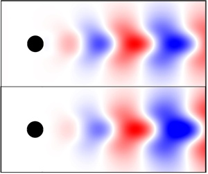
Figure 3. Spatial structures of the global modes in the cylinder wake at  $(a{,}c{,}e{,}g)$ $Re=40$ and $(b{,}d{,}f{,}h)$ $Re=80$. (a–d) The $y$-velocity perturbations (of the direct eigenvectors) show where the linear vortex-shedding modes are most active, (e,f) adjoint eigenvectors show where the modes are most affected by external forcing and (g,h) structural sensitivity regions show where the flow is most sensitive to perturbations. In (a–f), red (positive) and blue (negative) refer to $y$-velocity perturbations.
The direct eigenvectors indicate where the instability is most observable and hence where sensors could be placed. For controller design, we also need the adjoint eigenvectors, which indicate where actuators could be placed. The third row of figure 3 shows the adjoint eigenvectors (also in terms of the  $y$-component of velocity) from the model, calculated to leading order as in Juniper & Pier (Reference Juniper and Pier2015), and its comparison with the exact adjoint eigenvector, calculated by solving the adjoint of (2.2) (Giannetti & Luchini Reference Giannetti and Luchini2007). Finally, the last row of figure 3 shows the overlap between the direct and adjoint eigenvectors. This overlap, called the structural sensitivity region, indicates where the instability is generated, i.e. the wavemaker region (Giannetti & Luchini Reference Giannetti and Luchini2007). The square markers in the figure denote regions of maximal structural sensitivity, which is where a passive control device, such as a small control cylinder (Strykowski & Sreenivasan Reference Strykowski and Sreenivasan1990), would have the largest effect on the global instability (Giannetti & Luchini Reference Giannetti and Luchini2007); these results could be further improved by including the sensitivity to base-flow modifications, as shown by Marquet, Sipp & Jacquin (Reference Marquet, Sipp and Jacquin2008) and Pralits, Brandt & Giannetti (Reference Pralits, Brandt and Giannetti2010). The location of maximal structural sensitivity is predicted very accurately at $Re = 40$ and reasonably well at $Re = 80$. As is the case with the eigenvalue results, the errors increase as the flow becomes more non-parallel at higher $Re$.
$Re$.
4.3. Application to mean flow stability analysis
Linear global modes obtained from basic flow stability analysis are useful because they describe the evolution of infinitesimal perturbations in a flow (Tammisola et al. Reference Tammisola, Lundell, Schlatter, Wehrfritz and Söderberg2011). Such modes, however, often fail to accurately characterize the nonlinearly saturated finite-amplitude perturbations. This has led to interest in the application of stability analysis on the time-averaged (mean) flow; please see the early work of Malkus (Reference Malkus1956) and Stuart (Reference Stuart1958) as well as many subsequent studies focusing on cylinder wakes (Zielinska et al. Reference Zielinska, Goujon-Durand, Dušek and Wesfried1997; Pier Reference Pier2002; Noack et al. Reference Noack, Afanasiev, Morzyński, Tadmor and Thiele2003; Barkley Reference Barkley2006). In seminal work, Stuart (Reference Stuart1958) observed that the growth of perturbations is initially governed by linear theory, but once the perturbations become sufficiently large, they distort the mean flow such that an equilibrium state is reached where the energy transfer from the mean flow to the perturbations is balanced precisely by the energy dissipated via viscous effects. The idea, therefore, is that mean flow stability analysis can account for this energy transfer and can thus characterize the nonlinearly saturated finite-amplitude perturbations.
In figure 4(a), we present the basic flow (top half) and the mean flow (bottom half) for the cylinder wake at  $Re = 80$. Vortex shedding in the cylinder wake distorts the basic flow such that the recirculation bubble in the mean flow becomes shorter. Increasing $Re$ lengthens the recirculation bubble in the basic flow, but shortens it in the mean flow. This opposing trend was attributed by Zielinska et al. (Reference Zielinska, Goujon-Durand, Dušek and Wesfried1997) to a mean flow correction caused by the fundamental unstable mode. Consistent with this observation, figure 4(b) shows that while the region of local absolute instability grows in length with $Re$ for the basic flow, it shrinks in length with $Re$ for the mean flow. This highly nonlinear effect can also be seen in figure 4(e), where the deviation of the nonlinear vortex-shedding frequency from the linear global-mode frequency grows rapidly with $Re$. Again, the local stability results shown in figure 4(c) capture this frequency shift, which was also reported by Pier (Reference Pier2002). Finally, Barkley (Reference Barkley2006) performed a global stability analysis on the mean flow of a cylinder wake and found that (i) the obtained eigenfrequency exactly tracks the Strouhal number of nonlinear vortex shedding and (ii) the mean flow is marginally stable ( $\omega _{Gi} \approx 0$).

Figure 4.  $(a)$ Vorticity and streamlines in the basic (top) and mean (bottom) flow in the cylinder wake at $Re = 80$. Local absolute $(b)$ growth rate and $(c)$ frequency from the basic (blue) and mean (red) flow stability analyses. $(d)$ Growth rate of the linear global mode (blue line with solid circles) and that of the saturated mode from mean flow stability analysis (symbols). $(e)$ Frequency of the linear global mode (blue line with solid circles), frequency of the observed nonlinear vortex shedding from direct numerical simulations (red line) and frequency of the saturated mode from mean flow stability analysis (symbols).
An open question is whether the present framework can be extended to obtain mean flow global stability results similar to those reported by Barkley (Reference Barkley2006). To answer this, we apply the same procedure as explained above but with the basic flow replaced by the mean flow to obtain  $\omega _G$. The results are presented as symbols in figures 4(d) and 4(e). We find that the present framework slightly under-predicts the nonlinear frequency (figure 4e) but over-predicts the stabilizing effect of the mean flow distortion (figure 4d). Similar to the basic flow results, the mean flow results are better near the critical $Re$ but the errors increase as the flow becomes more non-parallel at higher $Re$.
$Re$.
From these results, we can conclude that the present framework is also applicable to mean flow stability analysis provided that the constraints for slow evolution in the streamwise direction are satisfied, much as they were for basic flow stability analysis. We must, however, caution that the mean flow is not generally a solution of the Navier–Stokes equations. The results from mean flow stability analysis, therefore, should be carefully interpreted. Sipp & Lebedev (Reference Sipp and Lebedev2007) showed that the mean flow is only marginally stable when the higher harmonics are not present; otherwise the energy transfer between different harmonics can affect the evolution of nonlinearly saturated perturbations, an effect that cannot be accounted for by mean flow stability analysis. We also note that another field of application of mean flow stability analysis is turbulent flows. The validity conditions for turbulent mean flow stability analysis have been provided by Beneddine et al. (Reference Beneddine, Sipp, Arnault, Dandois and Lesshafft2016) while the use of the present framework to model convective instabilities in a turbulent mean flow has been demonstrated by Gupta & Wan (Reference Gupta and Wan2019).
4.4. A three-dimensional flow: the flow past a sphere
Lastly, we demonstrate the applicability of the GLE for modelling the leading linear global mode and calculating the linear global stability results in the wake of a sphere at  $Re \equiv U_{\infty }D/\nu = 300$, where $D$ is the sphere diameter and $U_{\infty }$ is the free-stream velocity. This three-dimensional (3-D) flow undergoes a supercritical pitchfork bifurcation at $Re \approx 212$, after which it loses axisymmetry but gains planar symmetry (Fabre, Auguste & Magnaudet Reference Fabre, Auguste and Magnaudet2008). It then undergoes a supercritical Hopf bifurcation at $Re \approx 275$, transitioning to a limit cycle characterized by periodic vortex shedding (Tomboulides & Orszag Reference Tomboulides and Orszag2000). Direct global stability analysis of three-dimensional flows is still considered computationally expensive (Theofilis Reference Theofilis2011). Only recently have researchers reported direct global stability results for non-axisymmetric sphere wakes (Citro et al. Reference Citro, Tchoufag, Fabre, Giannetti and Luchini2016) and the corresponding WKB approximation (Siconolfi et al. Reference Siconolfi, Citro, Giannetti, Camarri and Luchini2017). Sphere wakes, therefore, represent a challenging yet verifiable flow on which the present GLE-based model can demonstrate its computational efficiency over the direct method as well as its advantage over the conventional WKB approximation involving analytic continuation of local stability results.
The basic flow for the sphere wake (figure 5a) is obtained using Nektar++ with 4700 hexahedral elements of polynomial order 5. The corresponding direct stability results (figure 5b) are obtained by discretizing the spatial operator using 587 500 points (see He et al. (Reference He, Burtsev, Theofilis, Zhang, Taira, Hayostek and Amitay2019) for details). The present method, by contrast, involves performing biglobal stability analysis at each  $x$-location, requiring spatial discretization in only the $y$- and $z$-directions. Here we use 36 points in $y$ from 0 to 3 and 72 points in $z$ from $-3$ to 3, all discretized on a Gauss–Lobatto–Chebyshev grid, as in § 4.1. Global stability results are then obtained by solving the GLE, which requires discretization in only the $x$-direction. The present method, therefore, effectively reduces a problem of size $\textit{O}(N_x\times N_y \times N_z)$ into $\textit{O}(N_x)$ problems of much smaller size $\textit{O}(N_y \times N_z)$. In principle, the application of the GLE remains the same as for the two-dimensional flows of § 4.1. In the implementation, however, we do not directly solve the third-order GLE (3.8), which requires higher spatial resolution for the biglobal stability calculations; instead we insert the solution of the GLE into (3.8) and minimize the residual in the neighbourhood of $X_c$.

Figure 5.  $(a)$ Vorticity and streamlines in a sphere wake at $Re = 300$. $(b)$ The linear global mode (top – exact, bottom – model) and its corresponding 3-D view in terms of isosurfaces of $z$-velocity perturbations (c – exact, h – model). Local absolute $(d)$ growth rate and $(e)$ frequency. Linear global mode $(\,f)$ $k_i$ and (g) $k_r$ obtained from the model (square markers denote $X_c$).
The global mode calculated from the GLE (bottom half of figure 5(b) and its 3-D view in figure 5h) is in good agreement with the directly calculated global mode (top half of figure 5(b) and its 3-D view in figure 5c), particularly in the region of local absolute instability (i.e. upstream of  $x \approx 2$). It is important to note that the linear global mode here varies more rapidly than the linear global modes in the two-dimensional wakes of § 4.1, particularly downstream of $x \approx 2$ (compare $k_r$ in figure 5(g) with those in the third row of figure 1). The first-order corrections to the mode shape (the second row of figure 3) are therefore expected to be large, explaining the mismatch between the model and exact linear global mode shapes in the downstream region. The eigenvalue calculated from the GLE ( $\omega _G = 0.79 + 0.08\textrm {i}$) is in good agreement with the direct results ( $\omega _G = 0.81 + 0.10\textrm {i}$) with less than $4\,\%$ error. Such agreement is reassuring considering that this sphere wake is much more non-parallel than the two-dimensional wakes considered in § 4.1. However, the global mode shapes calculated from analytic continuation of the local stability results of Siconolfi et al. (Reference Siconolfi, Citro, Giannetti, Camarri and Luchini2017) (figures 9(a) and 9(b) of their paper) match less well with the exact solutions, even in the region of local absolute instability (figures 9(e) and 9(f) of their paper).
Analytic continuation of local stability results to the complex plane is an ill-posed and ill-conditioned problem (Le Dizes et al. Reference Le Dizes, Huerre, Chomaz and Monkewitz1996). The WKB approximation of the stability results calculated by Siconolfi et al. (Reference Siconolfi, Citro, Giannetti, Camarri and Luchini2017) via analytic continuation is therefore impressive, particularly for the cylinder wake. For the sphere wake, however, analytic continuation becomes even more ill conditioned because this flow has a much smaller pocket of local absolute instability and is very non-parallel. Figure 5(d) shows that the pocket of local absolute instability in this flow extends to only  $x \approx 2$, downstream of which $\omega _{0i}$ quickly decreases to negative values. This implies that the local absolute instability results downstream of $x = 2$ quickly become irrelevant to the global mode. This can also be seen from figure 5(f) where $k_i$ is already very positive at $x = 2$ and consequently the global-mode amplitude quickly decreases downstream of $x \approx 2$. The functions $\omega _0$, $k_0$, $\omega _{kk}$ and their derivatives, which are required for analytic continuation, are therefore only available on a thin strip from $x = 0.5$ to $x \approx 2.0\text {--}3.0$. When analytic continuation is performed away from the strip in the complex plane, the errors are known to increase linearly with distance (normalized by the strip length) from the strip (Trefethen Reference Trefethen2020), thus limiting the use of analytic continuation for calculating the WKB approximation in such highly non-parallel flows.
We would like to take this opportunity to clarify the suitability of the expression used by Siconolfi et al. (Reference Siconolfi, Citro, Giannetti, Camarri and Luchini2017) to calculate the corrected global-mode shapes (figures 9(c) and 9(d) of their paper). In that expression, the spatial mode shape  $A(X)\exp \{\textrm {i}\varepsilon ^{-1}\int _X k(X',\omega _0^{g})\,\textrm {d}X'\}$ is corrected to first order as $A(X)\exp \left \{\textrm {i}\varepsilon ^{-1}\int _X k(X',\omega _G)\,\textrm {d}X'\right \}$ (see (4.1) of Siconolfi et al. Reference Siconolfi, Citro, Giannetti, Camarri and Luchini2017). This expression, however, is inconsistent with the WKB approximation in which the first-order corrections come from the variation in local stability results, such as the contribution of $\partial k(X,\omega _0^{g})/\partial x$. The first-order correction term $A(X)$ is given by Monkewitz et al. (Reference Monkewitz, Huerre and Chomaz1993), which explicitly includes $\partial k(X,\omega _0^{g})/\partial x$ among other terms (see (2.6)). Giannetti & Luchini (Reference Giannetti and Luchini2006) and Viola, Arratia & Gallaire (Reference Viola, Arratia and Gallaire2016) have presented solvability conditions for calculating such first-order correction terms for the forced response of locally convectively unstable flows. In the present framework, the correction term (2.6) is simplified as (3.5) and is included in the global mode obtained by solving the GLE. The caveat, however, is that there is no unique choice as to which physical variable $A(X)$ relates to. For example, in the sphere wake, it is related to the norm of the $z$-velocity perturbations. Because all the velocity perturbations follow nearly the same trend (i.e. reaching a maximum at around $x\approx 2$), the global-mode shape is not significantly affected by this choice.
5. Discussion
The present framework predicts the WKB approximation to global stability results for open shear flows. The implementation is straightforward as it involves determining the coefficients of the GLE from local stability analysis and avoids analytic continuation, which is an ill-posed and ill-conditioned problem. However, care must be taken to ensure that a smooth transition of the local wavenumber  $k$ occurs across $X_c$ (where the branch cut crosses the real $X$-axis), the boundaries do not significantly affect the results, and the imaginary part of $\omega _{kk1}$ remains mostly negative, satisfying causality (Chomaz et al. Reference Chomaz, Huerre and Redekopp1991). We find in § 4 that the error in the global stability predictions remains within approximately $5\,\%$ even for highly non-parallel flows at Reynolds numbers twice the critical values. Such levels of error in global stability calculations are acceptable because they can also arise from subtle differences in the BCs and fluid properties between experiments and simulations. The application of the present framework, therefore, also depends on its ability to handle such uncertainties. It can easily be demonstrated that the GLE-based model provides robust predictions so long as the large-scale features of the obtained coefficients remain unchanged. We have performed a quick test of this for the two-dimensional basic flow cases by adding to the coefficients $k_1$, $\omega _{k1}$ and $\omega _{kk1}$ random noise with a normal distribution and a standard deviation of $5.0\,\%$ (normalized by the spatial average of the coefficient). The resultant change in the $\omega _G$ predictions has a normalized standard deviation of under $0.5\,\%$ in all the cases studied.
The present framework also models the linear global modes in terms of the GLE, which have been the subject of many studies on flow control, e.g. Park et al. (Reference Park, Ladd and Hendricks1993), Roussopoulos & Monkewitz (Reference Roussopoulos and Monkewitz1996), Lauga & Bewley (Reference Lauga and Bewley2004), Bagheri et al. (Reference Bagheri, Henningson, Hœpffner and Schmid2009), Chen & Rowley (Reference Chen and Rowley2011) and Oehler & Illingworth (Reference Oehler and Illingworth2018). In particular, Lauga & Bewley (Reference Lauga and Bewley2004) and Bagheri et al. (Reference Bagheri, Henningson, Hœpffner and Schmid2009) studied the control of Ginzburg–Landau systems within the framework of linear time-invariant control theory. Later, Chen & Rowley (Reference Chen and Rowley2011) and Oehler & Illingworth (Reference Oehler and Illingworth2018) used a similar framework to explore optimal sensor and actuator placement in spatially developing flows. Such interest in the GLE arises from the fact that it can model the instabilities in spatially developing flows (Chomaz Reference Chomaz2005; Bagheri et al. Reference Bagheri, Henningson, Hœpffner and Schmid2009) at a cost low enough to make feedback control viable (Oehler & Illingworth Reference Oehler and Illingworth2018). Its applications, however, have until now remained only qualitative.
Here, we show that the GLE can quantitatively model flow instabilities in spatially developing flows, thus paving the way for the application of GLE-based control strategies to increasingly realistic flows. To realize this, however, one must first answer three questions: (i) How can the actuator inputs or the sensor outputs be transformed into the GLE variable (i.e.  $\varPsi$ in (3.2)) (Bagheri et al. Reference Bagheri, Henningson, Hœpffner and Schmid2009)? (ii) Can the GLE work on non-modal (Chen & Rowley Reference Chen and Rowley2011), quasi-periodic (Leclercq et al. Reference Leclercq, Demourant, Poussot-Vassal and Sipp2019) or multi-mode systems (Carini, Auteri & Giannetti Reference Carini, Auteri and Giannetti2015)? (iii) Can nonlinear effects be ignored (Leclercq et al. Reference Leclercq, Demourant, Poussot-Vassal and Sipp2019)? These questions are generally problem specific but have been addressed in great detail by Bagheri et al. (Reference Bagheri, Henningson, Hœpffner and Schmid2009). Furthermore, the issue of projecting the full system onto a reduced-order system has been addressed by Sipp & Schmid (Reference Sipp and Schmid2016).
6. Conclusions
Figures 2 and 3 capture the main achievements of this paper with regard to the prediction of global instability and the modelling of linear global modes in two-dimensional flows, while figures 4 and 5 extend the applicability to time-averaged and highly non-parallel three-dimensional flows, respectively. The two main strengths of the GLE-based model are that (i) it requires as input the basic flow in only a limited part of the domain in order to be able to robustly predict the linear global mode, and (ii) it is computationally efficient, reducing a triglobal stability problem to a series of simpler biglobal stability problems. The proposed model therefore opens up new possibilities for GLE-based linear control strategies to be directly applied to realistic flows. Crucially, the model makes accurate instability predictions possible even for flows that would otherwise be computationally intractable.
It is worth noting that although the present paper focuses on linear unforced global modes, the GLE has seen a wide range of applications in flow instability – and pattern formation in general. The GLE has been shown to be able to (i) qualitatively model fully nonlinear global modes (Pier & Huerre Reference Pier and Huerre1996; Pier et al. Reference Pier, Huerre, Chomaz and Couairon1998; Couairon & Chomaz Reference Couairon and Chomaz1999), (ii) capture secondary instabilities in wakes (Eckhaus and Benjamin–Feir instabilities) (Leweke, Provansal & Boyer Reference Leweke, Provansal and Boyer1993; Leweke & Provansal Reference Leweke and Provansal1994), (iii) predict the nature of bifurcations (Chomaz Reference Chomaz1992), (iv) predict the selection of solutions (van Saarloos & Hohenberg Reference van Saarloos and Hohenberg1990; Chomaz & Couairon Reference Chomaz and Couairon2000), (v) capture the transient growth and forced response of convectively unstable flows (Deissler Reference Deissler1987a; Cossu & Chomaz Reference Cossu and Chomaz1997; Gupta & Wan Reference Gupta and Wan2019) and (vi) capture turbulent bursts in boundary layers (Deissler Reference Deissler1987b) and transition to turbulence in open shear flows (Moon et al. Reference Moon, Huerre and Redekopp1983). Extending the model such that it can reproduce these features in real flows remains an important open challenge.
Acknowledgements
We would like to thank the anonymous reviewers for their valuable feedback. This work was supported by the National Natural Science Foundation of China (grant no. 91752201), the Shenzhen Science and Technology Innovation Committee (grant nos. JCYJ20170412151759222 and KQTD20180411143441009) and the Department of Science and Technology of Guangdong Province (grant no. 2019B21203001). We acknowledge support from the Centers for Mechanical Engineering Research and Education at MIT and SUSTech, as well as from the Center for Computational Science and Engineering at SUSTech. W.H. is supported by EPSRC, UK (grant no. EP/R037027/1). S.C. acknowledges support from the National Natural Science Foundation of China Basic Science Center Program (grant no. 11988102). L.K.B.L. is supported by the Research Grants Council of Hong Kong (grant nos. 16235716 and 16210418).
Declaration of interests
The authors report no conflict of interest.
Appendix A. Matrices in the global stability problem
 \begin{equation} \mathcal{L} = \begin{bmatrix} L - \textrm{i}\partial_xU & -\textrm{i}\partial_yU & -\textrm{i}\partial_zU & -\textrm{i}\partial_x\\ -\textrm{i}\partial_xV & L - \textrm{i}\partial_yV & -\textrm{i}\partial_zV & -\textrm{i}\partial_y\\ -\textrm{i}\partial_xW & -\textrm{i}\partial_yW & L -\textrm{i}\partial_zW & -\textrm{i}\partial_z\\ \partial_x & \partial_y & \partial_z & 0 \end{bmatrix},\quad \mathcal{B} = \begin{bmatrix} 1 & 0 & 0 & 0\\ 0 & 1 & 0 & 0\\ 0 & 0 & 1 & 0\\ 0 & 0 & 0 & 0 \end{bmatrix}, \end{equation}
where  $L = -\textrm {i}\boldsymbol {U}\boldsymbol {\cdot }\boldsymbol {\nabla } + ({\textrm {i}}/{Re})\Delta$.
 \begin{align} \mathcal{L}_0 &= \begin{bmatrix} D & -\textrm{i}\partial_yU & 0 & 0\\ 0 & D & 0 & -\textrm{i}\partial_y\\ 0 & 0 & D & -\textrm{i}\partial_z\\ 0 & \partial_y & \partial_z & 0 \end{bmatrix},\quad \mathcal{L}_1 = \begin{bmatrix} U & 0 & 0 & 1\\ 0 & U & 0 & 0\\ 0 & 0 & U & 0\\ \textrm{i} & 0 & 0 & 0 \end{bmatrix},\nonumber\\ &\quad \quad \mathcal{L}_2 = \begin{bmatrix} -\dfrac{\textrm{i}}{Re} & 0 & 0 & 0\\ 0 & -\dfrac{\textrm{i}}{Re} & 0 & 0\\ 0 & 0 & -\dfrac{\textrm{i}}{Re} & 0\\ 0 & 0 & 0 & 0 \end{bmatrix}, \end{align}
where  $D = ({\textrm {i}}/{Re})(\partial _y^{2}+\partial _z^{2})$.
 \begin{equation} \mathcal{L}_0^{n} = \begin{bmatrix} C - \textrm{i}\partial_xU + D & -\textrm{i}\partial_yU & -\textrm{i}\partial_zU & 0\\ -\textrm{i}\partial_xV & C - \textrm{i}\partial_yV + D & -\textrm{i}\partial_zV & -\textrm{i}\partial_y\\ -\textrm{i}\partial_xW & -\textrm{i}\partial_yW & C - \textrm{i}\partial_zW + D & -\textrm{i}\partial_z\\ 0 & \partial_y & \partial_z & 0 \end{bmatrix}, \end{equation}
where  $C = -\textrm {i}(V\partial _y + W\partial _z)$. It should be noted that the terms involving $V$,
$V$,  $W$, the derivative of the basic flow in $x$ (
$x$ ( $\partial _xU$, $\partial _xV$ and $\partial _xW$), and the $1/Re$ terms ( $D$ and the operator $\mathcal {L}_2$) are considered to be of order $\varepsilon$ or $\varepsilon ^{2}$. Consequently, these terms are not included in the zeroth-order solution of Monkewitz et al. (Reference Monkewitz, Huerre and Chomaz1993). Most other studies include the $1/Re$ terms in the zeroth-order solution but leave the other terms out. This, however, is a matter of choice. If these terms are accurately known, they can be included in the zeroth-order solution at no extra cost, as shown by Siconolfi et al. (Reference Siconolfi, Citro, Giannetti, Camarri and Luchini2017).


 Open access