


1 Introduction
Double diffusion occurs when the density of a fluid is a function of two scalars that diffuse at different rates. Our primary motivation is double diffusion in the ocean, so we will refer to the faster-diffusing scalar as temperature and to the slower-diffusing scalar as salt. Double diffusion can drive a variety of flows, including diffusive convection, salt fingering, thermohaline intrusions and thermohaline staircases (Turner Reference Turner1985; Schmitt Reference Schmitt1994; Radko Reference Radko2013), and may impact canonical flows, including gravity currents, plumes and Kelvin–Helmholtz billows (Smyth, Nash & Moum Reference Smyth, Nash and Moum2005; Konopliv & Meiburg Reference Konopliv and Meiburg2016; Dadonau, Partridge & Linden Reference Dadonau, Partridge and Linden2020). Here, we will analyse the energetics of double-diffusive fluids using the concepts of ‘background’ and ‘available’ potential energy.
The background potential energy (BPE) can be found by adiabatically sorting the density field into a monotonically decreasing function of height (Lorenz Reference Lorenz1955). The BPE is then defined as the potential energy associated with the sorted density field, and the available potential energy (APE) is the difference between the potential energy of the unsorted density and the BPE. The budgets for APE and BPE were first derived by Winters et al. (Reference Winters, Lombard, Riley and D’Asaro1995) for a single-component, incompressible, Boussinesq fluid. Winters et al. (Reference Winters, Lombard, Riley and D’Asaro1995) showed that energy can be transferred from APE to BPE, but not vice versa (and hence termed irreversible mixing), via a diapycnal (across surfaces of constant density) diffusive buoyancy flux. This framework was used to formalize the definition of mixing efficiency, an often-used concept in ocean mixing (e.g. Peltier & Caulfield Reference Peltier and Caulfield2003; Gregg et al. Reference Gregg, D’Asaro, Riley and Kunze2018). Here, we extend the framework from Winters et al. (Reference Winters, Lombard, Riley and D’Asaro1995) to include double-diffusive effects.
A local definition of APE was introduced by Tailleux (Reference Tailleux2013) and Scotti & White (Reference Scotti and White2014), which was further generalized to include compressibility, a nonlinear equation of state and an arbitrary number of scalar components (Tailleux Reference Tailleux2018b). Recently, Tailleux (Reference Tailleux2018a) derived a new expression for the local APE dissipation rate in a binary compressible fluid with a nonlinear equation of state and showed that in this case the APE dissipation is irreversible. Tailleux (Reference Tailleux2013, Reference Tailleux2018a,Reference Tailleuxb) included terms to represent diabatic heat and salt fluxes, but did not explicitly consider diffusion or double-diffusive effects. Here we will follow the derivation in Winters et al. (Reference Winters, Lombard, Riley and D’Asaro1995) and extend their analysis of the global APE and BPE budgets to include double diffusion.
Smyth et al. (Reference Smyth, Nash and Moum2005) considered the problem of double diffusion by applying the Winters et al. (Reference Winters, Lombard, Riley and D’Asaro1995) formulation to temperature and salinity separately, defining a background potential energy for each component by sorting temperature and salinity independently. While this approach is useful for quantifying irreversible mixing for each scalar, temperature and salinity do not have a gravitational potential energy separate from the fluid density. This approach also does not capture the single-component limit of equal molecular diffusivities. For example, consider a situation where non-zero horizontal temperature and salinity gradients are compensating such that the density depends only on the vertical coordinate. If the molecular diffusivities of each component are equal and the equation of state is linear, then the analysis of Winters et al. can be applied to the fluid density; if the density profile is stable, the APE will be zero. However, the APE calculated from the temperature and salinity individually will be non-zero.
Here we offer three main results. First, we consider the general criterion for the diapycnal buoyancy flux in a double-diffusive fluid and show that its sign can be expressed in terms of what we call the ‘gradient ratio’,  $G_{\unicode[STIX]{x1D70C}}\equiv (\unicode[STIX]{x1D6FC}|\unicode[STIX]{x1D735}T|)/(\unicode[STIX]{x1D6FD}|\unicode[STIX]{x1D735}S|)$, as well as the angle $\unicode[STIX]{x1D703}$ made between the scalar gradients (figure 1), and the ratio of the molecular diffusivities ( $\unicode[STIX]{x1D705}_{T},\unicode[STIX]{x1D705}_{S}$). Second, we extend the work of Winters et al. (Reference Winters, Lombard, Riley and D’Asaro1995) by deriving the volume-averaged APE and BPE budgets for an incompressible Boussinesq stratified fluid with a linear equation of state and two diffusing components. We show that the criterion for an up-gradient buoyancy flux obtained earlier can be related to a condition for a transfer of BPE to APE. Note that, while this result changes the interpretation of the partition between APE and BPE, we will still use the terms APE and BPE to refer to the standard definitions based on the sorted buoyancy. The criterion that we derive is useful for identifying when double diffusion qualitatively changes the energy transfers in a multiple-component fluid. Third, we generalize the evolution equation for the sorted buoyancy profile (Nakamura Reference Nakamura1996; Winters & D’Asaro Reference Winters and D’Asaro1996) for a double-diffusive fluid and relate an up-gradient diapycnal buoyancy flux to a negative effective diffusivity in sorted buoyancy coordinates. We then test our criteria using a simulation of salt fingering (figure 2) and show that the previously observed negative diffusivity of salt fingering (e.g. St. Laurent & Schmitt Reference St. Laurent and Schmitt1999) can be described in terms of $G_{\unicode[STIX]{x1D70C}}$ and $\unicode[STIX]{x1D703}$, generalizing the previous results of Veronis (Reference Veronis1965) and Garrett (Reference Garrett1982).
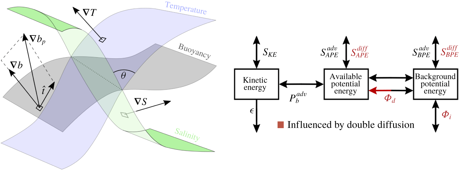
Figure 1. (a) A schematic to illustrate the angle made between surfaces of constant temperature and salinity. Generically the angle  $\unicode[STIX]{x1D703}(\boldsymbol{x},t)$ varies in space and time. (b) A schematic adapted from Winters et al. (Reference Winters, Lombard, Riley and D’Asaro1995) for a double-diffusive fluid. The arrows pointing up and down indicate energy exchanges with external and internal energy, respectively.
2 Results
2.1 Governing equations
We will consider the incompressible Boussinesq Navier–Stokes equations
 $$\begin{eqnarray}\displaystyle & \displaystyle \frac{\text{D}\boldsymbol{u}}{\text{D}t}=-\frac{\unicode[STIX]{x1D735}p}{\unicode[STIX]{x1D70C}_{0}}+b\hat{\boldsymbol{k}}+\unicode[STIX]{x1D735}\boldsymbol{\cdot }\unicode[STIX]{x1D749}, & \displaystyle\end{eqnarray}$$
 $$\begin{eqnarray}\displaystyle & \displaystyle \unicode[STIX]{x1D735}\boldsymbol{\cdot }\boldsymbol{u}=0, & \displaystyle\end{eqnarray}$$
 where  $\text{D}/\text{D}T=\unicode[STIX]{x2202}/\unicode[STIX]{x2202}t+\boldsymbol{u}\boldsymbol{\cdot }\unicode[STIX]{x1D735}$ denotes the material derivative and $\boldsymbol{u}=(u,v,w)$ is the velocity with respect to Cartesian coordinates $(x,y,z)$. The fluid pressure is $p$,
$p$,  $\hat{\boldsymbol{k}}$ is the unit vector in the $z$ direction, $b$ is the buoyancy and $\unicode[STIX]{x1D735}\boldsymbol{\cdot }\unicode[STIX]{x1D749}$ is the divergence of the viscous stress tensor. Additionally, we consider two advection–diffusion equations for the two stratifying elements, and a linear equation of state that relates these quantities to the fluid density, $\unicode[STIX]{x1D70C}$, and hence buoyancy, $b\equiv -g(\unicode[STIX]{x1D70C}-\unicode[STIX]{x1D70C}_{0})/\unicode[STIX]{x1D70C}_{0}$, where $g$ is the gravitational acceleration and $\unicode[STIX]{x1D70C}_{0}$ is a constant reference density. Specifically, these equations are
 $$\begin{eqnarray}\displaystyle & \displaystyle b=g(\unicode[STIX]{x1D6FC}T-\unicode[STIX]{x1D6FD}S), & \displaystyle\end{eqnarray}$$
 $$\begin{eqnarray}\displaystyle & \displaystyle \frac{\text{D}T}{\text{D}t}=\unicode[STIX]{x1D705}_{T}\unicode[STIX]{x1D6FB}^{2}T, & \displaystyle\end{eqnarray}$$
 $$\begin{eqnarray}\displaystyle & \displaystyle \frac{\text{D}S}{\text{D}t}=\unicode[STIX]{x1D705}_{S}\unicode[STIX]{x1D6FB}^{2}S. & \displaystyle\end{eqnarray}$$
 Note that  $T$ and $S$ can be viewed as generic diffusing scalars, with molecular diffusivities $(\unicode[STIX]{x1D705}_{T},\unicode[STIX]{x1D705}_{S})$.
2.2 Condition for an up-gradient buoyancy flux
By introducing a new variable  $b_{p}$, the buoyancy evolution equation can be written as
 $$\begin{eqnarray}\frac{\text{D}b}{\text{D}t}=\unicode[STIX]{x1D6FB}^{2}b_{p},\quad \text{where }b_{p}\equiv g(\unicode[STIX]{x1D6FC}\unicode[STIX]{x1D705}_{T}T-\unicode[STIX]{x1D6FD}\unicode[STIX]{x1D705}_{S}S).\end{eqnarray}$$
 We will refer to  $b_{p}$ as the ‘buoyancy flux potential’, since $\unicode[STIX]{x1D735}b_{p}$ is the diffusive buoyancy flux. As illustrated in figure 1, $\unicode[STIX]{x1D735}b_{p}$ is not necessarily in the same direction as $\unicode[STIX]{x1D735}b$ (unlike in a single-component fluid), which can result in a buoyancy flux along isopycnals (surfaces of constant density). We can divide the buoyancy flux into diapycnal and isopycnal components,
 $$\begin{eqnarray}\unicode[STIX]{x1D735}b_{p}=\underbrace{(\unicode[STIX]{x1D735}b_{p}\boldsymbol{\cdot }\hat{\boldsymbol{n}})\hat{\boldsymbol{n}}}_{diapycnal\;buoyancy\;flux}+\underbrace{(\unicode[STIX]{x1D735}b_{p}\boldsymbol{\cdot }\hat{\boldsymbol{t}})\hat{\boldsymbol{t}}}_{isopycnal\;buoyancy\;flux},\end{eqnarray}$$
 where  $\hat{\boldsymbol{n}}=\unicode[STIX]{x1D735}b/|\unicode[STIX]{x1D735}b|$ is the unit normal to the isopycnal surface, and $\hat{\boldsymbol{t}}$ is a unit vector tangent to the isopycnal surface, illustrated in figure 1.
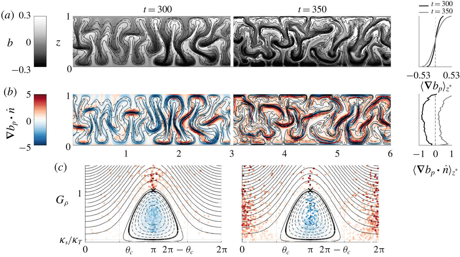
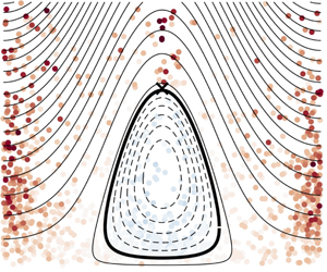
Figure 2. Buoyancy (a) and diapycnal buoyancy flux (b,c) from a two-dimensional simulation of salt fingering. Dashed and solid contours in panels (a,b) show temperature and salinity, respectively. Panels (c) are scatterplots of the diapycnal buoyancy flux (coloured as in (b)) in ( $G_{\unicode[STIX]{x1D70C}},\unicode[STIX]{x1D703}$) space. The panels to the right of (a,b) show the sorted height $(z^{\ast })$ averages of the panels and the initial profiles are indicated with a dashed line.
Introducing the gradient ratio  $G_{\unicode[STIX]{x1D70C}}\equiv (\unicode[STIX]{x1D6FC}|\unicode[STIX]{x1D735}T|)/(\unicode[STIX]{x1D6FD}|\unicode[STIX]{x1D735}S|)$, the diapycnal buoyancy flux can be written as
 $$\begin{eqnarray}\displaystyle \unicode[STIX]{x1D735}b_{p}\boldsymbol{\cdot }\hat{\boldsymbol{n}}=\frac{g^{2}\unicode[STIX]{x1D705}_{S}\unicode[STIX]{x1D6FD}^{2}|\unicode[STIX]{x1D735}S|^{2}}{|\unicode[STIX]{x1D735}b|}\left(\frac{\unicode[STIX]{x1D705}_{T}}{\unicode[STIX]{x1D705}_{S}}G_{\unicode[STIX]{x1D70C}}^{2}+\left(\frac{\unicode[STIX]{x1D705}_{T}}{\unicode[STIX]{x1D705}_{S}}+1\right)G_{\unicode[STIX]{x1D70C}}\cos \unicode[STIX]{x1D703}+1\right), & & \displaystyle\end{eqnarray}$$
 where  $\cos \unicode[STIX]{x1D703}=-\unicode[STIX]{x1D735}T\boldsymbol{\cdot }\unicode[STIX]{x1D735}S/(|\unicode[STIX]{x1D735}T||\unicode[STIX]{x1D735}S|)$ and $\unicode[STIX]{x1D703}(\boldsymbol{x},t)$ is the angle between the vectors $\unicode[STIX]{x1D735}T$ and $-\unicode[STIX]{x1D735}S$. The scalar angle is defined such that, when $\unicode[STIX]{x1D703}=0,2\unicode[STIX]{x03C0}$, the gradients in $T$ and $S$ point in opposing directions such that they contribute to the buoyancy gradient constructively. This definition implies that $\unicode[STIX]{x1D703}$ is also the angle made between the $T$ and $S$ isoscalar surfaces (see figure 1).
We will refer to the term in brackets in equation (2.8) as  $f(G_{\unicode[STIX]{x1D70C}},\unicode[STIX]{x1D703},\unicode[STIX]{x1D705}_{T}/\unicode[STIX]{x1D705}_{S})$. Explicitly
 $$\begin{eqnarray}f\left(G_{\unicode[STIX]{x1D70C}},\unicode[STIX]{x1D703},\frac{\unicode[STIX]{x1D705}_{T}}{\unicode[STIX]{x1D705}_{S}}\right)\equiv \frac{\unicode[STIX]{x1D705}_{T}}{\unicode[STIX]{x1D705}_{S}}G_{\unicode[STIX]{x1D70C}}^{2}+\left(\frac{\unicode[STIX]{x1D705}_{T}}{\unicode[STIX]{x1D705}_{S}}+1\right)G_{\unicode[STIX]{x1D70C}}\cos \unicode[STIX]{x1D703}+1.\end{eqnarray}$$
 The function  $f$ sets the sign of the diapycnal buoyancy flux, $\unicode[STIX]{x1D735}b_{p}\boldsymbol{\cdot }\hat{\boldsymbol{n}}$, since the other terms in equation (2.8) are positive definite. Therefore, a condition for an up-gradient diapycnal buoyancy flux is $f<0$. The dividing line between positive and negative diapycnal flux, $f=0$, is a quadratic equation in $G_{\unicode[STIX]{x1D70C}}$ and $\cos \unicode[STIX]{x1D703}$, plotted in bold in figure 2. The contours of $f$ are also plotted in figure 2. Since $G_{\unicode[STIX]{x1D70C}}$, $\unicode[STIX]{x1D705}_{T}$ and $\unicode[STIX]{x1D705}_{S}$ are positive, $\cos \unicode[STIX]{x1D703}$ is the only term in equation (2.9) that can be negative. Therefore, the relative orientation of the surfaces of constant $T$ and $S$ is of central importance to the sign of the diapycnal buoyancy flux. A Reynolds-averaged version of $f$ was derived as a term in the equation for the density variance by de Szoeke (Reference de Szoeke1998), who showed that negative values of this quantity can lead to the production of density variance. The significance of the condition in equation (2.9) to the APE and BPE budgets will be discussed in the next section.
When  $\unicode[STIX]{x1D703}=\unicode[STIX]{x03C0}$, the condition for a negative diapycnal buoyancy flux reduces to
 $$\begin{eqnarray}\unicode[STIX]{x1D735}b_{p}\boldsymbol{\cdot }\hat{\boldsymbol{n}}<0\quad \;\Longleftrightarrow \;\quad \frac{\unicode[STIX]{x1D705}_{S}}{\unicode[STIX]{x1D705}_{T}}<R_{\unicode[STIX]{x1D70C}}<1,\quad \text{where }R_{\unicode[STIX]{x1D70C}}\equiv \frac{\unicode[STIX]{x1D6FC}\unicode[STIX]{x0394}T}{\unicode[STIX]{x1D6FD}\unicode[STIX]{x0394}S}\end{eqnarray}$$
 is the density ratio. This is a well-known result in the double-diffusive literature (e.g. Veronis Reference Veronis1965; Garrett Reference Garrett1982; St. Laurent & Schmitt Reference St. Laurent and Schmitt1999; Radko Reference Radko2013). Therefore, equation (2.9) can be viewed as a generalization of equation (2.10), which includes horizontal  $T$ and $S$ gradients. Note that salt fingering instability occurs when $R_{\unicode[STIX]{x1D70C}}>1$ in the case of vertically aligned gradients such that the diffusive buoyancy flux will be down-gradient (Radko Reference Radko2013). However, as we will demonstrate below, equation (2.9) can be used to analyse the energetics of active salt fingering convection by considering the $T$ and $S$ gradients associated with individual salt fingers.
The third row of figure 2 shows contours of  $f(G_{\unicode[STIX]{x1D70C}},\unicode[STIX]{x1D703})$, where the region of $f<0$ is represented with dashed contours and the bounding line for this region is in bold. Superimposed are data from a simulation of salt fingers, which will be discussed below. The $\unicode[STIX]{x1D735}b_{p}\boldsymbol{\cdot }\hat{\boldsymbol{n}}<0$ region is bounded by a critical angle $\unicode[STIX]{x1D703}_{c}$, where
 $$\begin{eqnarray}\unicode[STIX]{x1D703}_{c}=\cos ^{-1}\left(\frac{-2\sqrt{\displaystyle \frac{\unicode[STIX]{x1D705}_{T}}{\unicode[STIX]{x1D705}_{S}}}}{\displaystyle \frac{\unicode[STIX]{x1D705}_{T}}{\unicode[STIX]{x1D705}_{S}}+1}\right)\quad \;\Longrightarrow \;\quad \frac{\unicode[STIX]{x03C0}}{2}<\unicode[STIX]{x1D703}_{c}\leqslant \unicode[STIX]{x03C0}.\end{eqnarray}$$
 For  $\unicode[STIX]{x1D705}_{T}=10^{-7}~\text{m}^{2}~\text{s}^{-1}$ and $\unicode[STIX]{x1D705}_{S}=10^{-9}~\text{m}^{2}~\text{s}^{-1}$, typical of the ocean, the critical angle is $\unicode[STIX]{x1D703}_{c}\simeq 100^{\circ }$. In the limit as $\unicode[STIX]{x1D705}_{T}/\unicode[STIX]{x1D705}_{S}\rightarrow 1$, the critical angle $\unicode[STIX]{x1D703}_{c}\rightarrow \unicode[STIX]{x03C0}$.
2.3 Potential energy budget
In this section we extend the framework of Winters et al. (Reference Winters, Lombard, Riley and D’Asaro1995) to include double-diffusive effects. Within a static volume  ${\mathcal{V}}$ with boundary ${\mathcal{S}}$, we can define the kinetic energy (2.12), potential energy (2.13), background potential energy (2.14) and available potential energy (2.15):
 $$\begin{eqnarray}\displaystyle & \displaystyle E_{KE}=\frac{\unicode[STIX]{x1D70C}_{0}}{2}\int _{{\mathcal{V}}}u^{2}+v^{2}+w^{2}\,\text{d}{\mathcal{V}}, & \displaystyle\end{eqnarray}$$
 $$\begin{eqnarray}\displaystyle & \displaystyle E_{PE}=-\unicode[STIX]{x1D70C}_{0}\int _{{\mathcal{V}}}bz\,\text{d}{\mathcal{V}}, & \displaystyle\end{eqnarray}$$
 $$\begin{eqnarray}\displaystyle & \displaystyle E_{BPE}=-\unicode[STIX]{x1D70C}_{0}\int _{{\mathcal{V}}}bz^{\ast }\,\text{d}{\mathcal{V}}, & \displaystyle\end{eqnarray}$$
 $$\begin{eqnarray}\displaystyle & \displaystyle E_{APE}=E_{PE}-E_{BPE}=\unicode[STIX]{x1D70C}_{0}\int _{{\mathcal{V}}}b(z^{\ast }-z)\,\text{d}{\mathcal{V}}, & \displaystyle\end{eqnarray}$$
 where  $z^{\ast }$ is the sorted buoyancy coordinate,
 $$\begin{eqnarray}z^{\ast }(\boldsymbol{x},t)=\frac{1}{A}\int _{{\mathcal{V}}^{\prime }}H(b(\boldsymbol{x},t)-b(\boldsymbol{x}^{\prime },t))\,\text{d}{\mathcal{V}}^{\prime },\end{eqnarray}$$
 with  $H$ the Heaviside function and $A$ the cross-sectional area of the volume ${\mathcal{V}}$. The sorted height $z^{\ast }(\boldsymbol{x},t)$ can be interpreted as the height of a fluid parcel after sorting the buoyancy field $b$ into a stable configuration, i.e. $b(z^{\ast })$ is the sorted buoyancy profile. Alternatively, $z^{\ast }(b)$ is the normalized volume of fluid with buoyancy less than $b$. In practice, $z^{\ast }$ can be calculated by integrating the probability density function of $b$ (Tseng & Ferziger Reference Tseng and Ferziger2001). Following the method outlined in Winters et al. (Reference Winters, Lombard, Riley and D’Asaro1995), the budgets of the energy components for a double-diffusive fluid are
 $$\begin{eqnarray}\displaystyle \frac{\text{d}E_{KE}}{\text{d}t} & = & \displaystyle -\underbrace{\oint _{{\mathcal{S}}}\left(p\boldsymbol{u}-\frac{1}{2}\unicode[STIX]{x1D70C}_{0}\boldsymbol{u}(u^{2}+v^{2}+w^{2})-\boldsymbol{u}\boldsymbol{\cdot }\unicode[STIX]{x1D749}\right)\boldsymbol{\cdot }\hat{\boldsymbol{n}}\,\text{d}{\mathcal{S}}}_{S_{KE}}\nonumber\\ \displaystyle & & \displaystyle +\,\unicode[STIX]{x1D70C}_{0}\underbrace{\int _{{\mathcal{V}}}bw\,\text{d}{\mathcal{V}}}_{P_{b}^{adv}}-\unicode[STIX]{x1D70C}_{0}\underbrace{\int _{{\mathcal{V}}}\unicode[STIX]{x1D70F}_{ij}\frac{\unicode[STIX]{x2202}u_{i}}{\unicode[STIX]{x2202}x_{j}}}_{\unicode[STIX]{x1D716}}\,\text{d}{\mathcal{V}},\end{eqnarray}$$
 $$\begin{eqnarray}\displaystyle & \displaystyle \frac{\text{d}E_{PE}}{\text{d}t}=\unicode[STIX]{x1D70C}_{0}\oint _{{\mathcal{S}}}\underbrace{(\!bz\boldsymbol{u}}_{S_{PE}^{adv}}-\underbrace{z\unicode[STIX]{x1D735}b_{p}\! )}_{S_{PE}^{diff}}\boldsymbol{\cdot }\,\hat{\boldsymbol{n}}\,\text{d}{\mathcal{S}}-\unicode[STIX]{x1D70C}_{0}\underbrace{\int _{{\mathcal{V}}}bw\,\text{d}{\mathcal{V}}}_{P_{b}^{adv}}+\unicode[STIX]{x1D70C}_{0}\underbrace{(A\overline{b_{p}})_{top}-(A\overline{b_{p}})_{bottom}}_{\unicode[STIX]{x1D6F7}_{i}},\quad & \displaystyle\end{eqnarray}$$
 $$\begin{eqnarray}\displaystyle & \displaystyle \frac{\text{d}E_{BPE}}{\text{d}t}=\unicode[STIX]{x1D70C}_{0}\oint _{{\mathcal{S}}}\underbrace{(\!\unicode[STIX]{x1D713}\boldsymbol{u}}_{S_{BPE}^{adv}}-\underbrace{z^{\ast }\unicode[STIX]{x1D735}b_{p}\! )}_{S_{BPE}^{diff}}\boldsymbol{\cdot }\,\hat{\boldsymbol{n}}\,\text{d}{\mathcal{S}}+\unicode[STIX]{x1D70C}_{0}\underbrace{\int _{{\mathcal{V}}}\frac{\text{d}z^{\ast }}{\text{d}b}(\unicode[STIX]{x1D735}b_{p}\boldsymbol{\cdot }\unicode[STIX]{x1D735}b)\,\text{d}{\mathcal{V}}}_{\unicode[STIX]{x1D6F7}_{d}}, & \displaystyle\end{eqnarray}$$
 $$\begin{eqnarray}\displaystyle \frac{\text{d}E_{APE}}{\text{d}t} & = & \displaystyle \unicode[STIX]{x1D70C}_{0}\underbrace{\oint _{{\mathcal{S}}}(bz-\unicode[STIX]{x1D713})\boldsymbol{u}\boldsymbol{\cdot }\hat{\boldsymbol{n}}\,\text{d}{\mathcal{S}}}_{S_{APE}^{adv}}+\unicode[STIX]{x1D70C}_{0}\underbrace{\oint _{{\mathcal{S}}}(z^{\ast }-z)\unicode[STIX]{x1D735}b_{p}\boldsymbol{\cdot }\hat{\boldsymbol{n}}\,\text{d}{\mathcal{S}}}_{S_{APE}^{diff}}-\unicode[STIX]{x1D70C}_{0}\underbrace{\int _{{\mathcal{V}}}bw\,\text{d}{\mathcal{V}}}_{P_{b}^{adv}}\nonumber\\ \displaystyle & & \displaystyle +\,\unicode[STIX]{x1D70C}_{0}\underbrace{(A\overline{b_{p}})_{top}-(A\overline{b_{p}})_{bottom}}_{\unicode[STIX]{x1D6F7}_{i}}-\unicode[STIX]{x1D70C}_{0}\underbrace{\int _{{\mathcal{V}}}\frac{\text{d}z^{\ast }}{\text{d}b}(\unicode[STIX]{x1D735}b_{p}\boldsymbol{\cdot }\unicode[STIX]{x1D735}b)\,\text{d}{\mathcal{V}}}_{\unicode[STIX]{x1D6F7}_{d}}.\end{eqnarray}$$
 These budgets can be derived by taking time derivatives of equations (2.12)–(2.15) and applying integration by parts. Additionally, one must use the relations  $\unicode[STIX]{x1D735}z^{\ast }=(\text{d}z^{\ast }/\text{d}b)\unicode[STIX]{x1D735}b$ and $\langle \text{d}z^{\ast }/\text{d}t\rangle _{z^{\ast }}=0$. By defining $\unicode[STIX]{x1D713}\equiv \int ^{b}z^{\ast }(s)\,\text{d}s$, we also use the relation $\unicode[STIX]{x1D735}\unicode[STIX]{x1D713}=z^{\ast }\unicode[STIX]{x1D735}b$. These equations are presented schematically in figure 1. Although we follow the derivation in Winters et al. (Reference Winters, Lombard, Riley and D’Asaro1995), these equations may also be derived by volume integrating the local APE budgets derived in Tailleux (Reference Tailleux2018b). The letter $S$ in equations (2.17)–(2.20) denotes a surface flux, with a superscript $adv$ denoting an advective flux, or $diff$ denoting a diffusive flux. The term $P_{b}^{adv}$ is the volume integral of the vertical advective buoyancy flux $bw$ and $\unicode[STIX]{x1D716}$ is the volume-integrated dissipation rate of kinetic energy. The term $\unicode[STIX]{x1D6F7}_{i}$ is the exchange between internal energy and potential energy. This term is discussed extensively in Konopliv & Meiburg (Reference Konopliv and Meiburg2016) in the context of the potential energy associated with the horizontally averaged buoyancy. In our volume-averaged formulation, $\unicode[STIX]{x1D6F7}_{i}$ only involves boundary quantities and in a turbulent flow we might expect $\unicode[STIX]{x1D6F7}_{i}$ to be small relative to $\unicode[STIX]{x1D6F7}_{d}$ (Peltier & Caulfield Reference Peltier and Caulfield2003).
Equations (2.17)–(2.20) differ from the single-component case presented in Winters et al. (Reference Winters, Lombard, Riley and D’Asaro1995) in the expressions for the diffusive surface terms  $S_{PE}^{diff}$, $S_{BPE}^{diff}$, $S_{APE}^{diff}$ and $\unicode[STIX]{x1D6F7}_{i}$ and the APE/BPE exchange term $\unicode[STIX]{x1D6F7}_{d}$, where $b_{p}$ now replaces $\unicode[STIX]{x1D705}b$. As a result, $\unicode[STIX]{x1D6F7}_{i}$ can take negative values in a fluid where the density increases with depth, which is not possible in a single-component fluid.
We define the quantity  $\unicode[STIX]{x1D719}_{d}$ as the integrand of $\unicode[STIX]{x1D6F7}_{d}$, i.e.
 $$\begin{eqnarray}\unicode[STIX]{x1D719}_{d}\equiv \frac{\text{d}z^{\ast }}{\text{d}b}\unicode[STIX]{x1D735}b_{p}\boldsymbol{\cdot }\unicode[STIX]{x1D735}b,\end{eqnarray}$$
 and using equation (2.8) the sign of  $\unicode[STIX]{x1D719}_{d}$ is set by the sign of $f(G_{\unicode[STIX]{x1D70C}},\unicode[STIX]{x1D703},\unicode[STIX]{x1D705}_{T}/\unicode[STIX]{x1D705}_{S})$ since $\text{d}z^{\ast }/\text{d}b>0$ by construction. There is a close connection between $\unicode[STIX]{x1D719}_{d}$ and the local diapycnal buoyancy flux $\unicode[STIX]{x1D735}b_{p}\boldsymbol{\cdot }\hat{\boldsymbol{n}}$.
Start by considering the average of an arbitrary continuous function,  $g(\boldsymbol{x},t)$, over a surface of constant $z^{\ast }$,
 $$\begin{eqnarray}\langle g(\boldsymbol{x},t)\rangle _{z^{\ast }}\equiv \frac{1}{A_{s}}\int _{{\mathcal{S}}^{\ast }}g(\boldsymbol{x},t)\,\text{d}{\mathcal{S}}^{\ast },\end{eqnarray}$$
 where  ${\mathcal{S}}^{\ast }$ is a surface with constant $z^{\ast }$ and $A_{s}$ is its area. Next, consider two isopycnals with buoyancy $b$ and $b+\unicode[STIX]{x0394}b$ and let $\unicode[STIX]{x0394}n$ and $\unicode[STIX]{x0394}z^{\ast }$ denote the perpendicular and sorted distances between the isopycnals. Then, taking the limit as $\unicode[STIX]{x0394}b\rightarrow 0$, we can write
 $$\begin{eqnarray}\displaystyle \langle g(\boldsymbol{x},t)\rangle _{z^{\ast }} & = & \displaystyle \lim _{\unicode[STIX]{x0394}b\rightarrow 0}\frac{1}{A_{s}}\frac{1}{\unicode[STIX]{x0394}z^{\ast }}\int _{{\mathcal{S}}^{\ast }}g(\boldsymbol{x},t)\frac{\unicode[STIX]{x0394}b}{\unicode[STIX]{x0394}n}\frac{\unicode[STIX]{x0394}z^{\ast }}{\unicode[STIX]{x0394}b}\unicode[STIX]{x0394}n\,\text{d}{\mathcal{S}}^{\ast }\nonumber\\ \displaystyle & = & \displaystyle \lim _{\unicode[STIX]{x0394}b\rightarrow 0}\frac{A}{A_{s}}\frac{1}{A\unicode[STIX]{x0394}z^{\ast }}\int _{\unicode[STIX]{x0394}{\mathcal{V}}^{\ast }}g(\boldsymbol{x},t)|\unicode[STIX]{x1D735}b|\frac{\text{d}z^{\ast }}{\text{d}b}\,\text{d}{\mathcal{V}}^{\ast }\nonumber\\ \displaystyle & = & \displaystyle \frac{A}{A_{s}}\frac{\text{d}z^{\ast }}{\text{d}b}\langle g(\boldsymbol{x},t)|\unicode[STIX]{x1D735}b|\rangle _{z^{\ast }},\end{eqnarray}$$
 where  $\unicode[STIX]{x0394}{\mathcal{V}}^{\ast }=A\unicode[STIX]{x0394}z^{\ast }$ is the volume between the isopycnal surfaces. Winters & D’Asaro (Reference Winters and D’Asaro1996) derived this relation for $g(\boldsymbol{x},t)=\unicode[STIX]{x1D705}|\unicode[STIX]{x1D735}b|$ (note that their result included a minus sign since they used density instead of buoyancy as the sorted variable).
Taking  $g(\boldsymbol{x},t)=\unicode[STIX]{x1D735}b_{p}\boldsymbol{\cdot }\hat{\boldsymbol{n}}$ and using equation (2.23) gives
 $$\begin{eqnarray}\langle \unicode[STIX]{x1D735}b_{p}\boldsymbol{\cdot }\hat{\boldsymbol{n}}\rangle _{z^{\ast }}=\frac{1}{A_{S}}\int _{{\mathcal{S}}^{\ast }}\unicode[STIX]{x1D735}b_{p}\boldsymbol{\cdot }\frac{\unicode[STIX]{x1D735}b}{|\unicode[STIX]{x1D735}b|}\,\text{d}{\mathcal{S}}^{\ast }=\frac{A}{A_{S}}\frac{\text{d}z^{\ast }}{\text{d}b}\langle \unicode[STIX]{x1D735}b_{p}\boldsymbol{\cdot }\unicode[STIX]{x1D735}b\rangle _{z^{\ast }}=\frac{A}{A_{S}}\langle \unicode[STIX]{x1D719}_{d}\rangle _{z^{\ast }},\end{eqnarray}$$
 and hence  $\langle \unicode[STIX]{x1D719}_{d}\rangle _{z^{\ast }}$ is related to the mean diapycnal buoyancy flux. Note that $\langle \unicode[STIX]{x1D719}_{d}\rangle _{z^{\ast }}$ and $\langle \unicode[STIX]{x1D735}b_{p}\boldsymbol{\cdot }\boldsymbol{n}\rangle _{z^{\ast }}$ have the same sign since $A$ and $A_{S}$ are positive. Similarly, we can write the magnitude of the isopycnal buoyancy flux $\unicode[STIX]{x1D735}b_{p}\boldsymbol{\cdot }\hat{\boldsymbol{t}}$ averaged across surfaces of constant $z^{\ast }$ as
 $$\begin{eqnarray}\langle \unicode[STIX]{x1D735}b_{p}\boldsymbol{\cdot }\hat{\boldsymbol{t}}\rangle _{z^{\ast }}=g\unicode[STIX]{x1D6FC}\unicode[STIX]{x1D6FD}|\unicode[STIX]{x1D705}_{T}-\unicode[STIX]{x1D705}_{S}|\frac{A}{A_{S}}\frac{\text{d}z^{\ast }}{\text{d}b}\langle |\unicode[STIX]{x1D735}T\times \unicode[STIX]{x1D735}S|\rangle _{z^{\ast }}.\end{eqnarray}$$
 The isopycnal buoyancy flux does not appear in the volume-integrated energy budget (2.17)–(2.20) and clearly vanishes for  $\unicode[STIX]{x1D705}_{S}=\unicode[STIX]{x1D705}_{T}$ or when $\unicode[STIX]{x1D735}T$ and $\unicode[STIX]{x1D735}S$ point in the same direction.
In a double-diffusive fluid, an up-gradient buoyancy flux can lead to  $\langle \unicode[STIX]{x1D719}_{d}\rangle _{z^{\ast }}<0$. In practice, it is easier to accurately measure gradients in temperature than salinity in the ocean (Klymak & Nash Reference Klymak and Nash2009). It is therefore convenient to recast this condition in terms of the temperature gradient,
 $$\begin{eqnarray}\langle \unicode[STIX]{x1D719}_{d}\rangle _{z^{\ast }}<0\quad \;\Longleftrightarrow \;\quad \left\langle \unicode[STIX]{x1D6FC}|\unicode[STIX]{x1D735}T|\frac{f\left(G_{\unicode[STIX]{x1D70C}},\unicode[STIX]{x1D703},\displaystyle \frac{\unicode[STIX]{x1D705}_{T}}{\unicode[STIX]{x1D705}_{S}}\right)}{G_{\unicode[STIX]{x1D70C}}\sqrt{f(G_{\unicode[STIX]{x1D70C}},\unicode[STIX]{x1D703},1)}}\right\rangle _{z^{\ast }}<0,\end{eqnarray}$$
 by noting that  $f(G_{\unicode[STIX]{x1D70C}},\unicode[STIX]{x1D703},1)=|\unicode[STIX]{x1D735}b|^{2}/(g^{2}\unicode[STIX]{x1D6FD}^{2}|\unicode[STIX]{x1D735}S|^{2})$ and applying (2.24). Although $G_{\unicode[STIX]{x1D70C}}$ and $\unicode[STIX]{x1D703}$ depend on $\unicode[STIX]{x1D735}S$, if these variables were parametrized, then equation (2.26) could be used with measurements of the temperature gradient to infer the sign of the average diapycnal buoyancy flux and provide insight into the exchange between APE and BPE.
The criteria in equations (2.9) and (2.26) can be applied to turbulent flows, including those in a doubly stable background stratification. We might expect vigorous turbulence to highly distort the scalar surfaces and influence the distribution of  $\unicode[STIX]{x1D703}$. If more points lie outside of the range of critical angles such that $\unicode[STIX]{x1D703}<\unicode[STIX]{x1D703}_{c}$ or $\unicode[STIX]{x1D703}>2\unicode[STIX]{x03C0}-\unicode[STIX]{x1D703}_{c}$, where $\unicode[STIX]{x1D703}_{c}$ is defined in (2.11), then we might anticipate that the average diapycnal buoyancy flux will be positive (down-gradient). This hypothesis will be tested below using simulations of salt fingering.
2.4 Evolution of sorted buoyancy
Following the derivation in Winters & D’Asaro (Reference Winters and D’Asaro1996) and Nakamura (Reference Nakamura1996) in the case of a single-component fluid, we can derive an equation for the evolution of the sorted buoyancy profile, averaged in  $z^{\ast }$ coordinates for a double-diffusive fluid:
 $$\begin{eqnarray}\displaystyle \frac{\unicode[STIX]{x2202}}{\unicode[STIX]{x2202}t}\langle b\rangle _{z^{\ast }}=\frac{\unicode[STIX]{x2202}}{\unicode[STIX]{x2202}z^{\ast }}\left(\left\langle \frac{\text{d}z^{\ast }}{\text{d}b}\unicode[STIX]{x1D735}b_{p}\boldsymbol{\cdot }\unicode[STIX]{x1D735}b\right\rangle _{z^{\ast }}\right)=\frac{\unicode[STIX]{x2202}}{\unicode[STIX]{x2202}z^{\ast }}\langle \unicode[STIX]{x1D719}_{d}\rangle _{z^{\ast }}. & & \displaystyle\end{eqnarray}$$
As in the single-component case, the divergence of the diapycnal buoyancy flux sets the time rate of change of the sorted buoyancy. A similar equation was derived by Paparella & von Hardenberg (Reference Paparella and von Hardenberg2012) for the evolution of the horizontally averaged buoyancy profile of a double-diffusive fluid, which evolved due to gradients in a combined advective and diffusive buoyancy flux. One advantage of equation (2.27) is that the diapycnal buoyancy flux does not directly involve the velocity field since the flux is purely diffusive.
The single-component version of equation (2.27) was used by Salehipour et al. (Reference Salehipour, Peltier, Whalen and MacKinnon2016) to propose a parametrization for the mixing efficiency in  $z^{\ast }$ coordinates, and Taylor & Zhou (Reference Taylor and Zhou2017) used this framework to develop a criterion for layer formation within a single-component stratified flow. Similarly, equation (2.27) could provide a pathway to parametrize double-diffusive flows. For example, it might be possible to parametrize $\langle \unicode[STIX]{x1D719}_{d}\rangle _{z^{\ast }}$ as a function of $\unicode[STIX]{x1D703}$ and $G_{\unicode[STIX]{x1D70C}}$, although this is beyond the scope of this paper.
As discussed in Nakamura (Reference Nakamura1996) and Winters & D’Asaro (Reference Winters and D’Asaro1996), equation (2.27) can be written in the form of a diffusion equation by defining an effective diffusivity for the sorted buoyancy,  $\unicode[STIX]{x1D705}_{b}(\boldsymbol{x},t)\equiv \langle \unicode[STIX]{x1D719}_{d}\rangle _{z^{\ast }}/(\text{d}b/\text{d}z^{\ast })$. Therefore, a negative mean diapycnal buoyancy flux implies a negative effective diffusivity, since buoyancy increases monotonically with height in sorted coordinates and hence $\text{d}b/\text{d}z^{\ast }\geqslant 0$. Previous work has shown that double-diffusive flows often develop a negative vertical turbulent diffusivity (e.g. Veronis Reference Veronis1965; St. Laurent & Schmitt Reference St. Laurent and Schmitt1999; Ruddick & Kerr Reference Ruddick and Kerr2003) and the expression for $\unicode[STIX]{x1D705}_{b}$ along with the definition of $\unicode[STIX]{x1D719}_{b}$ in equation (2.24) can be viewed as a generalization of this result when the averaging is applied in sorted buoyancy coordinates.
2.5 Application: Simulations of salt fingering
To demonstrate an application of the theory described above, we will consider a numerical simulation of a canonical double-diffusive flow: salt fingering. We time-stepped equations (2.1)–(2.5) in a two-dimensional ( $x$–
$x$– $z$) domain using a third-order Runge–Kutta scheme and second-order finite differences with an implicit Crank–Nicolson method for the viscous and diffusive terms. Details of the numerical method can be found in Bewley (Reference Bewley2012). The initial condition consists of a horizontally uniform temperature and salinity field with linear dependence on height, $z$. Here the fields are non-dimensionalized such that, for $z\in (0,1)$, the initial temperature field $T_{0}\in (0,1)$. Periodic boundary conditions are applied in $x$ with a non-dimensional domain width of $6$ to allow multiple salt fingers to form and interact. At the top and bottom of the domain $\boldsymbol{u}=0$, and temperature and salinity are set to their initial values. The profiles were set so that warm salty water overlies cold fresh water, a condition favourable for the formation of salt fingers. We used a density ratio of $R_{\unicode[STIX]{x1D70C}}=1.01$, close in value to $1$ to enable the most unstable mode to develop quickly (Kunze Reference Kunze2003). We used a diffusivity ratio of $\unicode[STIX]{x1D705}_{T}/\unicode[STIX]{x1D705}_{S}=20$, which implies $\unicode[STIX]{x1D703}_{c}\sim 115^{\circ }$, and a Prandtl number $Pr=\unicode[STIX]{x1D708}/\unicode[STIX]{x1D705}_{T}=1$ to give a similar critical angle to the oceanic case ( $\unicode[STIX]{x1D703}_{c}\sim 100$) without requiring a high resolution to resolve the Batchelor scales for the scalars. We used typical oceanic values in the linear equation of state $(\unicode[STIX]{x1D6FC},\unicode[STIX]{x1D6FD})=(3.9\times 10^{-5}~\text{}^{\circ }\text{C}^{-1},7.9\times 10^{-4}~\text{ppt}^{-1})$. The simulation was initiated with a small-amplitude random perturbation to the velocity. The results are qualitatively similar for a variety of parameter choices.
Figure 2(a) shows the temperature, salinity and buoyancy fields at two times. We only show half of the domain in  $x$ for each snapshot; however, the patterns are qualitatively similar across the domain. At $t=300$ (left panels) mature salt fingers are visible, and these fingers have broken down into a nonlinear chaotic flow at $t=350$ (right panels). The panel in the upper right shows the sorted buoyancy profile, which exceeds the bounds of the initial profile – a situation possible in a double-diffusive fluid. Figure 2(b) shows $\unicode[STIX]{x1D735}b_{p}\boldsymbol{\cdot }\hat{\boldsymbol{n}}$ at both times as well as the $z^{\ast }$ averages. Between the two times shown, the $z^{\ast }$ average of the diapycnal buoyancy flux changes sign. This appears to be due to the breakdown in the salt fingers, which otherwise preferentially increases salinity gradients.
A random subset of points are superimposed as a scatterplot of  $\unicode[STIX]{x1D735}b_{p}\boldsymbol{\cdot }\hat{\boldsymbol{n}}(G_{\unicode[STIX]{x1D70C}},\unicode[STIX]{x1D703})$ on top of $f$ contours in figure 2(c). The unperturbed initial conditions are denoted by a cross. As the salt fingers develop, local gradients in $T$ and $S$ increase. However, $|\unicode[STIX]{x1D735}S|$ increases faster than $|\unicode[STIX]{x1D735}T|$ and, as a result, $G_{\unicode[STIX]{x1D70C}}$ decreases. At $t=300$, when salt fingers are present, the scalar angle is primarily distributed around $\unicode[STIX]{x1D703}=\unicode[STIX]{x03C0}$, but enough points have $G_{\unicode[STIX]{x1D70C}}<1$ such that the diapycnal buoyancy flux is negative. At $t=350$, after the salt fingers have broken down, the distribution of angles becomes bimodal, with clustering of points near $\unicode[STIX]{x1D703}=\unicode[STIX]{x03C0}$ and $\unicode[STIX]{x1D703}=0,2\unicode[STIX]{x03C0}$. The magnitude of the diapycnal buoyancy flux is also maximum near these angles. At this time, the points with $\unicode[STIX]{x1D735}b_{p}\boldsymbol{\cdot }\hat{\boldsymbol{n}}>0$ near $\unicode[STIX]{x1D703}=0,2\unicode[STIX]{x03C0}$ more than compensate for the points near $\unicode[STIX]{x1D703}=\unicode[STIX]{x03C0}$, resulting in a positive mean diapycnal buoyancy flux.
This simulation illustrates how salt fingers distort the temperature and salinity contours such that  $|\unicode[STIX]{x1D735}S|$ increases faster than $|\unicode[STIX]{x1D735}T|$, leading to $G_{\unicode[STIX]{x1D70C}}<1$, and BPE conversion into APE on average. Once the flow becomes fully developed, the $T$ and $S$ gradients align such that $\unicode[STIX]{x1D703}$ is close to $0,2\unicode[STIX]{x03C0}$, and as a result the diapycnal buoyancy flux reverses sign and APE is converted into BPE on average. Although there is much left to explore, this example illustrates how the new criteria involving $G_{\unicode[STIX]{x1D70C}}$ and $\unicode[STIX]{x1D703}$ can be used to analyse the energetics of a double-diffusive flow.
3 Discussion and conclusion
Here, we extended the energetic framework of Winters et al. (Reference Winters, Lombard, Riley and D’Asaro1995), Winters & D’Asaro (Reference Winters and D’Asaro1996) and Nakamura (Reference Nakamura1996) to a double-diffusive fluid. In this framework, an up-gradient diapycnal buoyancy flux averaged in sorted height coordinates is equivalent to a negative buoyancy diffusivity for the sorted buoyancy profile and a transfer of energy from the background potential energy (BPE) to the available potential energy (APE).
We derived criteria for a transfer from BPE to APE in terms of the gradient ratio  $G_{\unicode[STIX]{x1D70C}}=\unicode[STIX]{x1D6FC}|\unicode[STIX]{x1D735}T|/(\unicode[STIX]{x1D6FD}|\unicode[STIX]{x1D735}S|)$, the angle $\unicode[STIX]{x1D703}$ between $\unicode[STIX]{x1D735}T$ and $\unicode[STIX]{x1D735}S$, and the ratio of molecular diffusivities, $\unicode[STIX]{x1D705}_{T}/\unicode[STIX]{x1D705}_{S}$ (see (2.9) and (2.26)). We applied these critera to salt fingering, an important mixing mechanism within the ocean. The criteria could be applied to ocean observations or direct numerical simulations in other contexts. Finally, we derived an evolution equation for the sorted buoyancy profile.
A transfer of energy from BPE to APE is not possible in a single-component fluid with a linear equation of state, where mixing is an ‘irreversible’ process. The finding that BPE can be converted into APE within double diffusion implies that some of the BPE can be made ‘available’ to drive fluid motion, and hence the interpretation of the APE from Winters et al. (Reference Winters, Lombard, Riley and D’Asaro1995) does not hold for a double-diffusive fluid. In particular this complicates the definition of ‘mixing efficiency’ as it is commonly calculated (Gregg et al. Reference Gregg, D’Asaro, Riley and Kunze2018). Nevertheless, the criteria in equation (2.26) provides a useful way to quantify the diffusive conversion of potential energy into a form that can be used to drive fluid motion in a double-diffusive fluid.
We formulated the results in this paper assuming molecular diffusion for temperature and salinity. However, a similar analysis could be applied using turbulent diffusivities, i.e. using the equations
 $$\begin{eqnarray}\frac{\text{D}T}{\text{D}t}=\unicode[STIX]{x1D735}\boldsymbol{\cdot }(K_{T}\unicode[STIX]{x1D735}T),\quad \frac{\text{D}S}{\text{D}t}=\unicode[STIX]{x1D735}\boldsymbol{\cdot }(K_{S}\unicode[STIX]{x1D735}S),\end{eqnarray}$$
 where  $K_{T}(\boldsymbol{x},t)$ and $K_{S}(\boldsymbol{x},t)$ are parametrized turbulent diffusivities. The condition (2.9) for $\unicode[STIX]{x1D735}b_{p}\boldsymbol{\cdot }\hat{\boldsymbol{n}}<0$ remains the same, with a replacement of molecular diffusivities $(\unicode[STIX]{x1D705}_{T},\unicode[STIX]{x1D705}_{S})$ with turbulent diffusivities $(K_{T},K_{S})$. Equations (2.17)–(2.20) are unchanged with $\unicode[STIX]{x1D735}b_{p}=g\unicode[STIX]{x1D6FC}K_{T}\unicode[STIX]{x1D735}T-g\unicode[STIX]{x1D6FD}K_{S}\unicode[STIX]{x1D735}S$, except that $\unicode[STIX]{x1D6F7}_{i}$ can no longer be written as a surface term. This allows our criterion in equation (2.9) to be applied to ocean models with parametrizations for $K_{T}$ and $K_{S}$, provided that a linear equation of state remains a good approximation. Although we have focused on fluids where the density is a function of two components, the results hold for an arbitrary buoyancy flux potential, $b_{p}$. In particular, this implies that our analysis could be extended to include more than two components.
Acknowledgements
The authors would like to thank Peter Haynes, Remi Tailleux and Catherine Vreugdenhil for very helpful discussions and comments on a draft of this paper. This work was supported by the Natural Environment Research Council (grant number NE/L002507/1).
Declaration of interests
The authors report no conflict of interest.


 Open access