


1. Introduction
In response to fluid flows, elastic structures observed in nature adjust their shapes to control the fluid loadings exerted on them. For example, leaves streamline, tree branches bend and grasses lump to reduce their frontal areas and mitigate the drag forces (Vogel Reference Vogel1984, Reference Vogel1989). Such adaptive deformation for the purpose of altering the fluid force, referred to as reconfiguration, has received considerable attention in the field of fluid–structure interactions. Since the pioneering investigations of Vogel (Reference Vogel1984, Reference Vogel1989), who elucidated the effectiveness of reconfiguration, the aerodynamic and hydrodynamic mechanisms responsible for the change in drag force induced by elastic deformation have been widely investigated. For instance, the effects of reconfiguration on the drag imposed on plants were examined experimentally using diverse species, and it has been revealed that the flow-induced deformation of vegetation reduces the drag force significantly in aquatic and land plants (Harder et al. Reference Harder, Speck, Hurd and Speck2004; de Langre, Gutierrez & Cossé Reference de Langre, Gutierrez and Cossé2012; Nepf Reference Nepf2012; Whittaker et al. Reference Whittaker, Wilson, Aberle, Rauch and Xavier2013). Moreover, by adopting simplified models such as flexible fibres and thin elastic plates, theoretical relationships between drag reduction and the deformation of elastic structures have been modelled for various flow conditions, including uniform flow (Alben, Shelley & Zhang Reference Alben, Shelley and Zhang2002; Gosselin, de Langre & Machado-Almeida Reference Gosselin, de Langre and Machado-Almeida2010; Luhar & Nepf Reference Luhar and Nepf2011; Hassani, Mureithi & Gosselin Reference Hassani, Mureithi and Gosselin2016) and unsteady flow (Leclercq & de Langre Reference Leclercq and de Langre2016; Luhar & Nepf Reference Luhar and Nepf2016; Leclercq & de Langre Reference Leclercq and de Langre2018; Zhang & Nepf Reference Zhang and Nepf2021).
Elastic leaves and branches form a porous tree and bend collectively in the wind (de Langre Reference de Langre2008; Gosselin Reference Gosselin2019). Like trees and grass canopies, poroelastic structures passively adapt their configurations when subjected to external flow, thereby changing the fluid forces. The reconfigured state and change in drag force of poroelastic structures were investigated experimentally over wide ranges of the porosity and Reynolds number for perforated strips (Guttag et al. Reference Guttag, Karimi, Falcón and Reis2018; Jin et al. Reference Jin, Kim, Cheng, Barry and Chamorro2020; Pezzulla et al. Reference Pezzulla, Strong, Gallaire and Reis2020) and for a three-dimensional poroelastic model in which a number of flexible filaments are radially attached to a rigid sphere (Gosselin & de Langre Reference Gosselin and de Langre2011). Poroelastic structures generally streamline and reduce the drag. However, the drag can increase under particular circumstances. For example, Gosselin & de Langre (Reference Gosselin and de Langre2011) showed that the drag of a poroelastic model increases when the Cauchy number (the ratio between the fluid force on the undeformed shape of the structure and the structure rigidity) is not sufficiently high to fully streamline the model. In addition, Jin et al. (Reference Jin, Kim, Cheng, Barry and Chamorro2020) reported that an elastic strip perforated with many holes could increase the drag force, despite its streamlined shape, when the porosity of the strip was sufficiently high. Because the flows penetrating the holes produce small recirculating regions immediately behind the bent strip, the region of maximum velocity deficit is located closer to the porous strip than to a non-porous strip, generating a larger drag.
Based on previous studies on the reconfiguration of poroelastic structures, this study investigates a poroelastic cluster, which is a single porous system composed of numerous elastic individuals with distinct spacing. The overall behaviour of this poroelastic cluster is determined by the individual actions of its constituents and the fluid-dynamic interaction between them. This collective behaviour is different from the behaviour of a perforated structure or a poroelastic medium, which is basically a continuum containing voids or pores. In nature, poroelastic clusters often exhibit extraordinary flight performances, and underlying aerodynamic mechanisms have been investigated with regard to their porous structure. For instance, by virtue of porosity in a low-Reynolds-number regime, bristled wings of several tiny insects could generate the aerodynamic forces comparable to those of common non-porous wings, even with almost one-tenth the mass (Sunada et al. Reference Sunada, Takashima, Hattori, Yasuda and Kawachi2002; Davidi & Weihs Reference Davidi and Weihs2012). Plumed seeds, another example of aerodynamic poroelastic clusters in nature, can fly a distance of several kilometres with centimetre sizes (Greene & Johnson Reference Greene and Johnson1990; Nathan et al. Reference Nathan, Katul, Horn, Thomas, Oren, Avissar, Pacala and Levin2002; Tackenberg, Poschlod & Kahmen Reference Tackenberg, Poschlod and Kahmen2003; Greene Reference Greene2005). Recently, Cummins et al. (Reference Cummins, Seale, Macente, Certini, Mastropaolo, Viola and Nakayama2018) revealed that the porous structure of the seeds enables a steady flight by generating a stable separated vortex ring. Furthermore, by means of high porosity, a three-dimensional poroelastic structure effectively traces unsteady flows better than spherical objects of the same size (Galler & Rival Reference Galler and Rival2021).
Despite many studies on the effects of porosity, the effects of deformation on the aerodynamic performance of poroelastic clusters remain unexplored. Because the drag force contributes enhancing the flight performance of freely flying poroelastic clusters in terms of long-distance flight (Tackenberg et al. Reference Tackenberg, Poschlod and Kahmen2003), it could be hypothesised that the free poroelastic cluster would deform to augment the drag force, in contrast to fixed elastic structures that reconfigure to mitigate fluid loadings. As a preliminary study, we numerically investigate the rearrangement of poroelastic clusters by adopting simplified two-dimensional models that contain the notable features of general poroelastic clusters. The term rearrangement is used throughout this study to emphasise the collective movement of individual elastic constituents that produces the overall deformation of the poroelastic cluster. The changes in constituent distribution and drag force are examined by varying porosity and elasticity in the quasi-steady state, which is more closely related to long-distance flight than the initial transient state. In § 2, our simplified model for the poroelastic cluster and numerical method are described. In § 3.1, we discuss a characteristic flow phenomenon around the cluster, which dominates its rearrangement process. The effects of the flow phenomenon on the changes in cylinder arrangement and drag with respect to porosity and elasticity are explained by examining the force components of the cluster in § 3.2. A new variable that incorporates the effects of elasticity and porosity is introduced to characterise the rearrangement in § 3.3. Finally, concluding remarks are presented in § 4.
2. Problem description
2.1. Model and parameters
For the investigation of porous structures composed of multiple entities, two-dimensional simplification has often been adopted. For instance, a dandelion seed was modelled as a permeable disc (Casseau et al. Reference Casseau, de Croon, Izzo and Pandolfi2015; Ledda et al. Reference Ledda, Siconolfi, Viola, Camarri and Gallaire2019), and a three-dimensional bristled wing was represented by a linear array of two-dimensional circular cylinders with gaps (Jones et al. Reference Jones, Yun, Hedrick, Griffith and Miller2016; Lee & Kim Reference Lee and Kim2020, Reference Lee and Kim2021; Wu, Liu & Sun Reference Wu, Liu and Sun2021). Despite simplicity in the configurations, the underlying fluid-dynamic mechanisms were elucidated effectively in terms of identifying the flow behaviour around the porous structure or the fluid-dynamic interaction between multiple constituents. Similarly, as a simplified two-dimensional poroelastic cluster, we introduce a collection of circularly aligned cylinders where each cylinder is elastically mounted at its own centre (figure 1a). Our simplified model captures the salient features of general poroelastic clusters, where elastic individuals with distinct spacings congregate to form a single porous system.

Figure 1. (a) Simplified two-dimensional poroelastic cluster model with seven elastically mounted cylinders, (b) computational domain and (c) five poroelastic clusters (A7, A20, A39, A64 and A95).
Each cylinder has a diameter of  $d$ and a mass of $m$, and the cluster is subjected to a uniform fluid flow of velocity $U$ and density $\rho _f$. To realise diverse porosities within the cluster, the number of constituent cylinders, $N_C$, is varied while the outermost diameter of the cluster $D$ is restricted to $21d$ (figure 1a). The clusters with $N_C = 7$, 20, 39, 64 and 95 are denoted as A7, A20, A39, A64 and A95, respectively (figure 1c). For each model, the cylinders are arranged in layers of concentric circles, with one cylinder at the centre. The positions of the cylinders are determined such that they are located as evenly as possible, following the approach of Nicolle & Eames (Reference Nicolle and Eames2011). The porosity of the model is represented by the solid fraction $\phi = N_Cd^2/D^2$, which indicates the portion of the area occupied by the cylinders within the circular boundary of the cluster (Nicolle & Eames Reference Nicolle and Eames2011; Chang & Constantinescu Reference Chang and Constantinescu2015; Taddei, Manes & Ganapathisubramani Reference Taddei, Manes and Ganapathisubramani2016; Kingora & Sadat Reference Kingora and Sadat2022). By definition, $\phi$ increases with $N_C$, and $\phi = 1$ corresponds to an impervious cylinder of diameter $D$. The values of $\phi$ for our clusters are presented in table 1.
Table 1. Number of cylinders  $N_C$ and solid fraction $\phi ({=}N_Cd^2/D^2)$ for five poroelastic clusters (A7, A20, A39, A64 and A95).

To numerically simulate the flow-induced motion of cylinders, a mass–spring–damper system is separately adopted for each cylinder, and each cylinder is elastically mounted at its own initial centre. In the two-dimensional domain, only the  $x$- and $y$-directional translations of the cylinder are considered because actual long and thin hairs in three-dimensional space mostly bend under the flow, but rarely twist. For each cylinder, the springs for the $x$- and $y$-directional translations are decoupled (figure 1a). All springs are assumed to have an identical stiffness of $k$. The motion of each cylinder is then governed by the dimensionless equation
 \begin{equation} m^*\ddot{Q^*_i} + c^*\dot{Q^*_i} + k^* {Q^*_i} = f^*_i, \end{equation}
where  $m^* = m/(\rho _f d^2)$, $c^* = c/(\rho _f U d)$ and $k^* = k/(\rho _f U^2)$ are dimensionless parameters for the mass, damping coefficient and spring stiffness of a cylinder, respectively. Here $Q^*_i$ is the $i$-coordinate of the dimensionless position for the cylinder centre with respect to its own initial location, and is normalised by the cylinder diameter $d$, where $i$ denotes the $x$- or $y$-component; $\ddot {Q^*_i}$ and $\dot {Q^*_i}$ correspond to the dimensionless acceleration and velocity of the cylinder, respectively; $f^*_i$, which is normalised by $\rho _f U^2 d$, is the $i$-component of the dimensionless fluid force vector exerted on the cylinder. Because the current study is primarily aimed at understanding the effects of elasticity (spring stiffness $k^*$) on the rearrangement and drag force of the poroelastic cluster, $m^*$ is fixed to unity ( $m^* = 1$). In addition, damping is not considered ( $c^* = 0$) because our interest is behaviours in the quasi-steady state after the initial transient state passes; the damping does not affect the steady solution of a mass–spring–damper system. Although our poroelastic cluster models are composed of multiple cylinders, we confirmed that the results of the quasi-steady state remained consistent, regardless of the $c^*$ value.
The spring stiffness  $k^*$ of the individual cylinders ranges between 0.3 and 1.0 ( $k^* = 0.3$, 0.5, 0.7 and 1.0). Because a similar trend is observed as $k^*$ increases beyond 1.0, the maximum value is limited to 1.0. As $k^*$ becomes greater, the cylinders behave more stiffly. For example, an extreme case of $k^* = 10$ shows aerodynamic behaviours very similar to the rigid counterpart with $k^* = \infty$. The minimum value of $k^*$ is limited to 0.3 because most poroelastic models produce unrealistic motions for smaller values of $k^*$; a few cylinders revolve around adjacent cylinders, which is unlikely to occur in poroelastic clusters in nature. Moreover, when $k^* < 0.3$, the shape of the cluster becomes excessively irregular, and collisions occur between the cylinders with large $\phi$. As we aim to reveal the general effects of the rearrangement, extreme circumstances with irregular rearrangement are not addressed in the present study. The chosen range of $k^*$ is sufficient to comprehensively understand the effects of $k^*$. In addition, a rigid cluster with $k^*=\infty$, in which the cylinders are stationary, is also considered for comparison. Here $k^*$ represents the ratio between the elastic restoring force and the fluid loading, similar to the reciprocal of the Cauchy number $C_Y$ that is generally used to characterise the reconfiguration of elastic or poroelastic structures (de Langre Reference de Langre2008; Gosselin et al. Reference Gosselin, de Langre and Machado-Almeida2010; Gosselin & de Langre Reference Gosselin and de Langre2011; Luhar & Nepf Reference Luhar and Nepf2016; Guttag et al. Reference Guttag, Karimi, Falcón and Reis2018; Pezzulla et al. Reference Pezzulla, Strong, Gallaire and Reis2020). Because the spring stiffness $k$ is varied in this study, we employ $k^*$ instead of $C_Y$ ( ${=}1.0\unicode{x2013}3.3$) to represent the force ratio in a straightforward manner.
The poroelastic cluster is subjected to a free stream of constant velocity  $U$. The rearrangement of the poroelastic cluster in the quasi-steady state remains unaffected even if the free stream is unsteady in the initial transient phase, prior to attaining the constant velocity. This consistency justifies the use of the constant velocity $U$ for the velocity profile to examine the quasi-steady state. In nature, poroelastic clusters usually reside in the low-Reynolds-number regime of $Re = O(10)$ or less, where $Re$ is based on the diameter of entities comprising the cluster (Greene & Johnson Reference Greene and Johnson1990; Santhanakrishnan et al. Reference Santhanakrishnan, Robinson, Jones, Low, Gadi, Hedrick and Miller2014). In this $Re$ regime, hydrodynamic interaction between multiple bodies within the cluster is so strong that the flow hardly passes through spacings between the bodies (Nawroth et al. Reference Nawroth, Feitl, Colin, Costello and Dabiri2010; Lee & Kim Reference Lee and Kim2017; Lee, Lee & Kim Reference Lee, Lee and Kim2020). Through preliminary tests, we determined the Reynolds number that sufficiently realised such flow phenomenon. The Reynolds number $Re_d$ for a single cylinder in our model is fixed to be 10: $Re_d = U d/\nu = 10$. Accordingly, the Reynolds number $Re_D\ ({=}UD/\nu )$ for the whole cluster is 210.
2.2. Numerical method
To compute the interaction between the flow and the multiple cylinders, an in-house code is constructed by building a new OpenFOAM library that implements the direct-forcing immersed boundary method (IBM) (Mahravan, Lahooti & Kim Reference Mahravan, Lahooti and Kim2023). Our in-house code numerically solves the governing equations for a two-dimensional incompressible laminar flow, which are given as
 \begin{gather} \boldsymbol{\nabla} \boldsymbol{\cdot} \boldsymbol{u} = 0, \end{gather}
 \begin{gather}\dfrac{\partial \boldsymbol{u}}{\partial t} + (\boldsymbol{u} \boldsymbol{\cdot}\boldsymbol{\nabla}) \boldsymbol{u} ={-} \frac{1}{\rho_f} \boldsymbol{\nabla} p + \nu {\nabla}^2\boldsymbol{u} + \boldsymbol{f}_{\!\!IB}, \end{gather}
where  $\boldsymbol {u}$ is the flow velocity vector, $p$ is the pressure and $\nu$ is the kinematic viscosity of the fluid. The force $\boldsymbol{f}_{\!\!IB}$ per unit mass in (2.2b) refers to a source term satisfying the continuity condition across the immersed boundaries (Uhlmann Reference Uhlmann2005). Here $\boldsymbol{f}_{\!\!IB}$ is formulated by transferring variables between the Eulerian coordinate of the fluid domain $\varOmega$ and the Lagrangian coordinate $\varPi$ that formulates the immersed boundary composed of Lagrangian markers.
At the beginning of each time step, the momentum equation (2.2b) is first solved without  $\boldsymbol{f}_{\!\!IB}$ to compute an intermediate Eulerian velocity $\tilde {\boldsymbol {u}}$. Interpolating $\tilde {\boldsymbol {u}}$ through the discrete Dirac delta function $\delta$ (Roma, Peskin & Berger Reference Roma, Peskin and Berger1999), the preliminary velocity at the Lagrangian markers is obtained: $\tilde {\boldsymbol {U}}(\boldsymbol {X}) = \int _{\varOmega } \tilde {\boldsymbol {u}}(\boldsymbol {x}) \delta (\boldsymbol {x} - \boldsymbol {X}) \,\textrm {d}V$. The Lagrangian force $\boldsymbol {F}_{IB}$ is then determined using the Lagrangian velocity $\boldsymbol {U}$ from the previous time step as $\boldsymbol {F}_{IB} = \textrm {d}(\boldsymbol {U}-\tilde {\boldsymbol {U}})/\textrm {d}t$. Finally, the Eulerian force $\boldsymbol{f}_{\!\!IB}$ in (2.2b) is calculated by transferring $\boldsymbol {F}_{IB}$ from the surrounding Lagrangian markers to the Eulerian nodes:
 \begin{equation} \boldsymbol{f}_{\!\!IB} = \int_{\varPi} \boldsymbol{F}_{IB}(\boldsymbol{X}) \delta (\boldsymbol{X} - \boldsymbol{x})\,\textrm{d}s. \end{equation}
With  $\boldsymbol{f}_{\!\!IB}$ included, the governing equations (2.2a) and (2.2b) are solved using the PISO algorithm modified by Constant et al. (Reference Constant, Favier, Meldi, Meliga and Serre2017). This modified algorithm allows stable and accurate calculations when implemented with the IBM embedded in OpenFOAM. The time is discretised using the first-order implicit Euler scheme. For spatial discretisation, the second-order Gauss scheme is used for all terms except the convection term, for which the second-order linear upwind scheme is applied.
After solving the flow field, the fluid forces exerted on Lagrangian markers are calculated again at the same time step. The fluid forces are then summed for the markers comprising the surface of a cylinder, yielding the total fluid force  $\boldsymbol {f}$ exerted on the cylinder. Therefore, the dimensionless force term $f^*_i$ on the right-hand side of (2.1) corresponds to the dimensionless form of $\boldsymbol {f}$: $f^*_i = f_i / \rho _f U^2 d$, where $i=x$ or $y$. At the end of the time step, the velocity of the cylinder is updated by discretising and solving (2.1) with regard to the velocity, and the position of the cylinder is updated from the obtained velocity.
The rectangular fluid domain spans  $[-16D, 32D] \times [-16D, 16D]$, and the origin of the coordinate system coincides with the initial centre of the cylinder cluster (figure 1b). The free stream enters the left boundary of the domain, and the pressure outlet condition of $p = 0$ and a zero normal gradient of velocity is imposed at the right boundary downstream. The top and bottom boundaries are set to have zero normal gradients for the pressure and slip conditions for the velocity, i.e. slip-wall boundary conditions.
Figure 2 illustrates the grid sizes and layouts, in which the immersed boundaries of the cylinders are marked with black and white circles in panels (b-ii) and (b-iii), respectively. As shown in figure 2(a), the entire fluid domain is divided into nine regions having different grid sizes  $\Delta x$. Each region consists of uniform square grids, and the grid size doubles in the neighbouring outer region, following the approach of Constant et al. (Reference Constant, Favier, Meldi, Meliga and Serre2017); see figure 2(b-i) for the overall layout of the constructed grids. In our numerical algorithm, all immersed boundaries move inside the fluid region with uniform grids of the same size. However, enlarging the finest region to enclose the movements of all cylinders increases the computational cost significantly. To resolve this issue, adaptive mesh refinement (AMR) is applied to generate the finest grids of $\Delta x_f = 0.02d$ near the poroelastic clusters by refining the surrounding grids of $\Delta x = 0.04d$. The refinement is performed only when any cylinder inside the finest region approaches an interface with the outer region of $\Delta x = 0.04d$; that is, only when any cylinder is about to escape the region of $\Delta x_f = 0.02d$. The finest region, which is indicated by the blue circle in figure 2(b-iii), is large enough to fully encompass the cluster. The finest grids around two cylinders are presented in figure 2(b-ii) to visualise that the size of the finest grid is much smaller than the diameter of a single cylinder. The size of the discretised Lagrangian markers for the immersed boundaries is identical to that of the finest grid in the fluid domain, $\Delta s = 0.02d$.

Figure 2. (a) Grid size of nine fluid subdomains and (b) computational grid layouts. Panel (b-i) demonstrates the overall layout of constructed grids, whereas panels (b-ii) and (b-iii) depict the grid layouts around two cylinders and the whole cluster, respectively. The black circle in panel (a) corresponds to the blue circle in panel (b-iii).
A series of tests are conducted to confirm the feasibility and accuracy of our numerical set-up. As a first step to validate that our in-house code solves the flow-induced motion of cylinders accurately, the vortex-induced vibration of two tandem circular cylinders under a uniform flow is considered. To match the conditions with those of Bao et al. (Reference Bao, Huang, Zhou, Tu and Han2012), the centre of the downstream cylinder is located 5 $d$ downstream from the centre of the upstream cylinder. Both cylinders have the same diameter $d$ and undergo two-degree-of-freedom motion in which the cylinder oscillates on the $xy$-plane. The Reynolds number $Re_d = 150$ and mass coefficient $m^* = 2$ match those of Bao et al. (Reference Bao, Huang, Zhou, Tu and Han2012) as well. Over a broad range of reduced velocity $U_r = U/(f_N d)$, where natural frequency $f_N = {1}/{2{\rm \pi} }(k/m)^{1/2}$, the maximum amplitudes in the $x$-direction ( $X_{max}/d$) and $y$-direction ( $Y_{max}/d$) are compared in figures 3(a) and 3(b), respectively. For both cylinders, our results are in good agreement with the previous results, ensuring that the flow-induced motion of cylinders can be accurately simulated by our numerical set-up.

Figure 3. Comparison of maximum amplitudes (a)  $X_{max}/d$ and (b) $Y_{max}/d$ with respect to reduced velocity $U_r$ for two tandem cylinders ( $m^* = 2, Re_d = 150$) undergoing vortex-induced vibration. (c) Comparison of time-averaged drag coefficient $\bar {C}_D$ with respect to solid fraction $\phi$ for a stationary cluster at $Re_d = 100$.
Moreover, the accuracy in solving the interaction between multiple bodies and a free stream is evaluated. The drag forces exerted on the circular array of stationary cylinders are compared with those reported by Nicolle & Eames (Reference Nicolle and Eames2011). Along with identical cluster configurations, the Reynolds number based on the diameter of a cylinder matches as  $Re_d = 100$. The total drag force $F_x$ acting on the cylinder array is represented as a sum of $x$-directional forces exerted on all cylinders: $F_x(t) = \sum _{j = 1}^{N_C} f_{x,j}(t)$. Because $F_x(t)$ fluctuates periodically at this $Re_d$, the time-averaged drag coefficient of the cluster is defined as
 \begin{equation} \bar{C}_D = \frac{1}{T} \int^{t_0+T}_{t_0} \frac{F_x (t)}{\dfrac{1}{2}\rho_f U^2 D} \textrm{d}t, \end{equation}
where  $T$ is the period of $F_x(t)$ and $t_0$ is a reference time. Figure 3(c) shows that our results match those of Nicolle & Eames (Reference Nicolle and Eames2011) with averaged difference less than 2 %, and our numerical set-up reliably computes multi-body problems.
Convergence tests are also performed to ensure that our solutions are independent of grid and time step sizes. The convergence is evaluated with the time history of  $F^*_x$, which is the sum of the dimensionless forces exerted on every cylinder in the $x$-direction ( $F^*_x = \sum _{j = 1}^{N_C} f^*_{x,j}$), for the A39 model with $k^* =$ 0.5. For grid convergence test, four cases with different finest grid sizes of $\Delta x_f = 0.01d$, 0.02 $d$, 0.04 $d$ and 0.08 $d$ are compared. Figure 4(a) indicates that the solution clearly converges for the case of $\Delta x_f = 0.02d$, and thus the finest grid size is chosen to be $\Delta x_f = 0.02d$ for all simulations. In addition, the time step size is varied for the same cluster model: $\Delta t = 0.001d/U$, 0.002 $d/U$, 0.004 $d/U$ and 0.008 $d/U$ (figure 4b). The time histories of $F^*_x$ show that the solution is hardly affected when $\Delta t \leqq 0.004d/U$. Accordingly, $\Delta t = 0.004d/U$ is chosen for all simulations.

Figure 4. Comparison of total  $x$-directional force $F^*_x$ of the A39 model ( $k^* = 0.5$) for (a) four different finest grid sizes of $\Delta x_f = 0.01d$, 0.02 $d$, 0.04 $d$ and 0.08 $d$ and (b) four different time step sizes of $\Delta t = 0.001d/U$, 0.002 $d/U$, 0.004 $d/U$ and 0.008 $d/U$. The inset in panel (b) presents $F^*_x$ for a short period of $tU/d = 14\unicode{x2013}18$ to clearly demonstrate the convergence with respect to $\Delta t$.
3. Results and discussion
3.1. Rearrangement and hydrodynamic blockage
When the cylinders comprising the poroelastic cluster are continuously exposed to a uniform free stream of constant velocity, they reach the quasi-steady state with negligible motion after undergoing notable movements in the initial transient state. In the quasi-steady state, the cylinders rearrange in such a way that the overall shape of the cluster expands in the direction normal to the incoming flow. In other words, the rearrangement of the poroelastic cluster enlarges its frontal area, causing the generation of a larger overall drag force, compared with the rigid cluster of  $k^*=\infty$ in which the frontal area remains unchanged. Figure 5 depicts this phenomenon in a simplified manner. Note that the degree of rearrangement and the magnitude of the drag force in figure 5(b) are exaggerated to some extent to more distinctly contrast the rigid and poroelastic clusters. In this section, we examine the characteristic flow phenomenon that is mainly responsible for this unique and counter-intuitive behaviour of the poroelastic cluster, where the frontal area expanded under the flow augments the drag.

Figure 5. Schematics of the overall configurations and flow patterns for (a) a rigid cluster and (b) a poroelastic cluster in the quasi-steady state. The black and grey arrows indicate the drag force  $F_x$ imposed on the clusters and streamlines, respectively. The red dashed line represents the boundary of the cluster.
To quantify the amount of rearrangement in terms of the frontal area normal to the flow, the frontal area is defined as a  $y$-directional length $L_y$ of the boundary encompassing the poroelastic cluster. Because the cylinders are not circularly positioned in the quasi-steady state due to the rearrangement, the boundary is fitted to an ellipse (red dashed line in figure 6a). The ellipse is first fitted using the centres of the outermost cylinders via direct least-squares fitting (Fitzgibbon, Pilu & Fisher Reference Fitzgibbon, Pilu and Fisher1999), and then the two major ellipse axes are expanded by $d/2$ with respect to the ellipse centre; $d/2$ is the radius of each cylinder. The fitted ellipse accurately depicts the outer boundary of the rearranged cluster. The frontal area $L_y$, which is the distance between the uppermost and lowermost points of the ellipse, is made dimensionless using the initial cluster diameter $D$ in figure 1(a) ( $L^*_y = L_y / D$); thus, $L^*_y = 1$ corresponds to the frontal area of a rigid cluster. The drag force of a cluster is defined as the total sum of the $x$-directional fluid forces exerted on all cylinders; the cluster drag $F^*_x = \sum _{j = 1}^{N_C} f^*_{x,j}$, where $f^*_x$ is the $x$-component of the dimensionless force imposed on a single cylinder ( $f^*_x = f_x/\rho _f U^2 d$). The quasi-steady state is defined as the state in which the values of $L^*_y$ and $F^*_x$ change less than 0.5 % over a dimensionless time period of $tU/d = 10$. In all cases considered herein, the quasi-steady state satisfied such a condition at $tU/d =$ 200. Thus, the following results presented for $L^*_y$ and $F^*_x$ correspond to this instant.

Figure 6. (a) Rearranged poroelastic clusters in the quasi-steady state for five models with  $k^* = 0.3$. The ellipse (red dashed line) is fitted to represent the boundary of the cluster. (b) Frontal area $L^*_y$ and (c) drag $F^*_x$ of the cluster in the quasi-steady state with respect to the solid fraction $\phi$. (d) Ratio of the poroelastic cluster drag over the rigid cluster drag, $F^*_x/F^*_{x,{rigid}}$, with respect to $L^*_y$.
Regarding the A7 model, which has the smallest solid fraction of  $\phi = 0.02$ (table 1), the frontal area $L^*_y \approx$ 1 for $k^* = 0.3$–1.0 (figure 6b), and the cluster drag $F^*_x$ is very similar to that of the rigid counterpart (figure 6c). However, for $\phi >$ 0.02, $L^*_y$ and $F^*_x$ are distinctly greater than those of the rigid counterparts, regardless of $k^*$. The frontal area and the cluster drag exhibit the same trend. As $\phi$ increases, both $L^*_y$ and $F^*_x$ increase and then decrease, having a peak at some intermediate value of $\phi$, and are consistently greater for smaller $k^*$. The maxima of both $L^*_y$ and $F^*_x$ for the poroelastic clusters occur at $\phi = 0.09$ and $k^* = 0.3$. In this condition, $L^*_y$ and $F^*_x$ are 8.6 % and 19.2 % greater than their values in the rigid counterpart, respectively. On the other hand, when the drag coefficient $C_D$ is calculated using the frontal area $L_y$ as a characteristic length scale ( $C_D = 2F_x/\rho _fU^2L_y$), $F^*_x$ and $C_D$ exhibit identical trends with respect to $\phi$ and $k^*$. Although the drag force experienced by the cluster can be expressed by either $F^*_x$ or $C_D$, $F^*_x$ is used in our analysis. In contrast to $F^*_x$, $C_D$ includes $L_y$ in its denominator, and thus the effect of the frontal area change induced by the rearrangement on the drag, which is one of the main interests in this study, cannot be captured directly by $C_D$.
To clarify the relation between the frontal area and the drag augmentation, we define the extent of drag increment as the ratio of the drag force experienced by a poroelastic cluster to that of a rigid cluster,  $F^*_x/F^*_{x,{rigid}}$. According to figure 6(d), $F^*_x/F^*_{x,{rigid}}$ tends to increase linearly with $L^*_y$, implying that the drag of the poroelastic cluster is strongly affected by the frontal area; other poroelastic clusters with different sizes also follow this linear relation as reported in figure 14(a) of the Appendix. The linear relation between the drag force and the frontal area is general for non-porous structures isolated alone. In this sense, the results in figure 6(d) suggest that the fluid-dynamic phenomenon, which is responsible for enlarging the frontal area and, thus, augmenting the drag, makes multiple cylinders function as a collective group in which entities interact cohesively, rather than as independent entities.
In the low-Reynolds-number regime of  $O$(10) or less, strong viscous diffusion forms shear layers around the separated bodies which are thick enough to create virtual fluid barriers inside the gaps between the separated bodies. These barriers consequently interrupt the flow penetrating the gaps (Nawroth et al. Reference Nawroth, Feitl, Colin, Costello and Dabiri2010; Lee & Kim Reference Lee and Kim2017; Lee, Lahooti & Kim Reference Lee, Lahooti and Kim2018). This phenomenon, namely hydrodynamic blockage, is more effective when $Re$ is smaller or the bodies are located closer together (Davidi & Weihs Reference Davidi and Weihs2012; Lee & Kim Reference Lee and Kim2020; Lee et al. Reference Lee, Lee and Kim2020). Similarly, for our clusters of $Re_d = 10$, the streamwise velocity inside the cluster indicates the emergence of hydrodynamic blockage, and the effect of the blockage strengthens as the solid fraction increases (figure 7). For the smallest $\phi = 0.02$ with the largest spacing between the cylinders, most of the incoming flow penetrates the gaps within the cluster at almost the same speed. At intermediate values of $\phi = 0.05$ and 0.09, the internal flow within the cluster diminishes gradually, as indicated by the reduced streamwise velocity and the smaller number of streamlines, and the incoming flow starts to detour around the cluster. Finally, at high solid fractions of $\phi = 0.15$ and 0.22, the hydrodynamic interaction between the cylinders is so dominant that the penetrating flow almost disappears; the velocity is almost zero inside the cluster. Thus, the incoming flow mostly curves around the outer edge of the cluster.

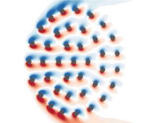
Figure 7. Contours of streamwise velocity in the quasi-steady state for five cluster models with different solid fractions  $\phi$ ( $k^* = 0.3$). Streamwise velocity is normalised as $u_x/U$. In each panel, streamlines of the incoming flow are illustrated on velocity contours.
To elaborate the effects of hydrodynamic blockage on the fluid forces imposed on the cylinders and the resultant rearrangement, a representative distribution of the fluid forces is visualised in figure 8 for the poroelastic clusters with  $k^* = 0.3$. When most of the incoming flow passes through the gaps between the cylinders ( $\phi = 0.02$), all cylinders are subjected to similar magnitudes of the fluid force (figure 8a). However, even with the weakest hydrodynamic blockage, the drag force $f^*_x$ of a cylinder in the cluster is notably smaller than that of a single isolated cylinder, $f^*_{x,{single}}$. For example, at $k^* = 0.3$, $f^*_x$ averaged over all the cylinders is equal to 0.71 $f^*_{x,{single}}$. In contrast, for the clusters with larger $\phi$, for which the flow is diverted by the development of virtual fluid barriers, the cylinders experience different fluid forces depending on their positions, and clear spatial variations in the fluid forces appear (figure 8b–e). At intermediate solid fractions ( $\phi = 0.05, 0.09$), the fluid forces exerted on the cylinders at the rear of the cluster become smaller than for those at the front compared with $\phi = 0.02$. Accordingly, by the development of hydrodynamic blockage, cylinders experience significantly reduced drag forces compared with $f^*_{x,{single}}$. For clusters with $k^* = 0.3$, $f^*_x$ averaged over all the cylinders is half of $f^*_{x,{single}}$ at $\phi = 0.05$ and further decreases to $0.30f^*_{x,{single}}$ at $\phi = 0.09$. Moreover, for high solid fractions ( $\phi = 0.15, 0.22$), the rear cylinders rarely experience any fluid force, whereas the front cylinders are still subjected to noticeable fluid forces. In common, when the hydrodynamic blockage is in effect, the outer cylinders that are directly exposed to the detouring flow encounter stronger fluid forces than the inner cylinders.

Figure 8. Magnitude and direction of fluid force  $\boldsymbol {f}^*$ exerted on each cylinder for five cluster models with different solid fractions $\phi$ ( $k^* = 0.3$). The red solid line denotes the force vector of each cylinder, and the horizontal red solid line at the bottom right of the figure indicates the magnitude of $|\boldsymbol {f}^*| = 1$.
Furthermore, whereas the flow passing through the cluster exerts a fluid force along almost the entire  $x$-direction for the sparsely distributed cluster (figure 8a), the flow that detours under the hydrodynamic blockage effect induces remarkable $y$-directional fluid forces for the more densely distributed clusters (figure 8b–e). The cylinders are rearranged to be symmetric with respect to the $x$-axis because of the flow symmetry through and around the cluster, as shown in figure 7. Thus, for a pair of cylinders symmetrically located between the upper and lower sides of the cluster, the magnitudes of the force vectors are equal, but their orientations are opposite in the $y$-direction. Although the distributions of the rearranged cylinders and the fluid forces are not perfectly symmetric with respect to the $x$-axis, the degree of asymmetry with respect to the $x$-axis is extremely small, and the distributions can be regarded symmetric. Moreover, the angle between the force vector and the $x$-axis is greater for the outer cylinders than for the inner cylinders on the front side. Accordingly, the cylinders experience $y$-directional motions during the rearrangement process, with greater movements of the outer cylinders. By virtue of the hydrodynamic blockage of which the degree is determined by the solid fraction, the frontal area of the rearranged poroelastic cluster becomes greater than that of the rigid cluster, eventually leading to an increase in cluster drag, as reported in figure 6(b–d).
The rearrangement of the poroelastic cluster is noteworthy in that the drag force is augmented through the enlargement of the frontal area under the flow. Although the drag increment has been reported for the reconfigured poroelastic strip (Jin et al. Reference Jin, Kim, Cheng, Barry and Chamorro2020) and poroelastic system composed of elastic filaments radially attached to a centre sphere in spherical form (Gosselin & de Langre Reference Gosselin and de Langre2011), the underlying mechanisms differ from our model. Although the drag of the poroelastic strip increases under certain conditions (Jin et al. Reference Jin, Kim, Cheng, Barry and Chamorro2020), the drag increment is because of a specific flow pattern behind the strip rather than the enlargement of the frontal area; the strip streamlines under a flow and its frontal area decreases. The streamlined reconfiguration of the poroelastic system of Gosselin & de Langre (Reference Gosselin and de Langre2011), which generally contributes to drag reduction, could increase the drag when all the elastic filaments are not fully streamlined at a low Cauchy number. However, the poroelastic system reconfigures primarily by the bending of independent filaments, and the effects of porosity on drag augmentation appear to be rather minor. In contrast, the rearrangement of our poroelastic clusters is achieved by the hydrodynamic blockage between constituents, and they exhibit different behaviours with respect to the solid fraction, yielding an optimal solid fraction for the cluster drag.
As a drag-based flier, the flight performance of a poroelastic cluster is mainly evaluated with the flight distance that is crucially affected by aerodynamic drag. The horizontal wind mainly induces a dispersion, and the updraft, which exerts the aerodynamic force against the gravity, sustains the dispersion in the air (Tackenberg et al. Reference Tackenberg, Poschlod and Kahmen2003). Because the poroelastic cluster can generate greater drag by enlarging its frontal area, it is expected to prolong flight duration compared with the rigid cluster, thereby enabling to fly longer distances. In addition, we suppose that the flight stability of the poroelastic cluster would not significantly differ from that of the rigid cluster. In the high-Reynolds-number (high- $Re$) regime, vortex shedding may occur behind the cluster, and the surrounding flow responds more sensitively to structural modifications or flow disturbances than in the low- $Re$ regime. In such conditions, the expansion of the frontal area would further intensify the flow instability, leading to unstable flight. However, in the low- $Re$ regime where the poroelastic cluster can take advantage of hydrodynamic blockage in enlarging the frontal area, the flow around the cluster remains stable as shown in figure 7, and the enlargement of the frontal area would not significantly affect the flight stability in comparison with the rigid cluster.
3.2. Force components of the poroelastic cluster
In § 3.1, a characteristic flow behaviour that causes the rearrangement of the poroelastic cluster was identified, namely hydrodynamic blockage. Here, we discuss how hydrodynamic blockage affects the frontal area  $L^*_y$ and cluster drag $F^*_x$ with respect to porosity (solid fraction $\phi$) and elasticity (spring stiffness $k^*$), using the force components acting on the cylinders. First, as $\phi$ increases, the drag force of the rigid and poroelastic clusters increases and then decreases for all $k^*$, exhibiting the maximum $F^*_x$ at certain values of $\phi$ (figure 6c). The rigid cluster presents a peak $F^*_x$ of 12.01 at $\phi = 0.05$, and $F^*_x$ attains a maximum for all poroelastic clusters at $\phi = 0.09$, where $F^*_x = 13.98$, 13.36, 13.12 and 12.86 for $k^* = 0.3$, 0.5, 0.7 and 1.0, respectively.
The increase and subsequent decrease in the cluster drag with respect to the solid fraction has been generally observed for arrays of static cylinders over a wide range of the Reynolds number (Chang & Constantinescu Reference Chang and Constantinescu2015; Taddei et al. Reference Taddei, Manes and Ganapathisubramani2016; Tang et al. Reference Tang, Yu, Shan, Chen and Su2019, Reference Tang, Yu, Shan, Li and Yu2020; Kingora & Sadat Reference Kingora and Sadat2022). However, less is known about the fluid-dynamic mechanism responsible for the presence of an optimal porosity that maximises the cluster drag. For example, Chang & Constantinescu (Reference Chang and Constantinescu2015) and Tang et al. (Reference Tang, Yu, Shan, Li and Yu2020) reported that the peak drag appeared between two solid-fraction regimes characterised by weak interaction between cylinders (low  $\phi$) and strong interaction that induces global vortex shedding behind the cylinder array (high $\phi$), respectively. However, as illustrated in figure 7, the periodic vortex shedding does not occur behind our poroelastic clusters at low $Re$. In addition, Kingora & Sadat (Reference Kingora and Sadat2022) employed a physical concept known as sheltering effect, which is similar to the effect of hydrodynamic blockage in our study, in order to analyse the spatial variation of fluid forces depending on the cylinder locations. However, the sheltering effect indicates a decrease in mean flow within the cylinder array, without specifically addressing the hydrodynamic interaction between multiple bodies by strong viscous diffusion, and it was not adopted to explain the drag experienced by the entire cylinder array. In this study, the mechanism that accounts for the appearance of an optimal $\phi$ is inferred by analysing the effects of hydrodynamic blockage on the cluster drag.
Whereas the degree of hydrodynamic blockage strengthens monotonically with an increase in the solid fraction  $\phi$, the cluster drag $F^*_x$ does not exhibit a monotonic change over $\phi$ due to the hydrodynamic blockage effect. If the hydrodynamic blockage is absent, the increase in $\phi$ produces an effect that is hydrodynamically equivalent to that of simply increasing $N_C$, which causes the cluster drag to increase. However, once the virtual fluid barrier interrupts the penetration of the incoming flow, the rear cylinders encounter little incoming flow, and thus increasing $\phi$ does not function equivalently as increasing $N_C$. As $F^*_x$ decreases with increasing $\phi$ for $\phi \geqq 0.09$, where the flow behaviour is predominated by the hydrodynamic blockage, it could be conjectured that the blockage yields an effect equivalent to that of decreasing $N_C$. To comprehensively understand how the hydrodynamic blockage affects the cluster drag, drag components are analysed in terms of the flow fields around the cluster.
We decompose the drag  $f_x$ of a single cylinder into the drag $f_{x,v}$ due to viscous stress $\boldsymbol {\tau }$ and the drag $f_{x,p}$ due to pressure $p$ as
 \begin{equation} f_x = f_{x,v} + f_{x,p} = \int_{S} \boldsymbol{n} \boldsymbol{\cdot} \boldsymbol{\tau}|_x\, \textrm{d}S + \int_{S} -p \boldsymbol{n}|_x\, \textrm{d}S, \end{equation}
where  $S$ is the surface of a cylinder and $\boldsymbol {n}$ is the unit normal vector out of $S$. Both components of the cylinder drag are made dimensionless using $\rho _f$, $U$ and $d$ as $f^*_{x,v} = f_{x,v} / \rho _f U^2 d$ and $f^*_{x,p} = f_{x,p} / \rho _f U^2 d$. The viscous and pressure drag forces on a cluster are defined in the same manner as the cluster drag $F^*_x$; thus, $F^*_{x,v} = \sum _{j=1}^{N_C} (f^*_{x,v})_j$ and $F^*_{x,p} = \sum _{j=1}^{N_C} (f^*_{x,p})_j$, respectively, where $F^*_{x,v} + F^*_{x,p} = F^*_x$. Similar to $F^*_x$, $F^*_{x,v}$ and $F^*_{x,p}$ increase and then decrease with respect to $\phi$, reaching a maximum at the same value of $\phi = 0.09$ (figure 9). The changes in $F^*_{x,v}$ and $F^*_{x,p}$ are analysed using vorticity fields (figure 10a,b) and pressure fields (figure 10c,d), respectively, near to the clusters of $\phi = 0.02$ (minimum), 0.09 (optimum) and 0.22 (maximum) with $k^* = 0.3$ as representative cases. The vorticity field is considered for $F^*_{x,v}$ because the viscous stress tensor $\boldsymbol {\tau }$ is linearly related to the vorticity $\boldsymbol {\omega }$ on the cylinder surface $S$ according to $\boldsymbol {n} \boldsymbol{\cdot} \boldsymbol {\tau } = -\mu \boldsymbol {n} \times \boldsymbol {\omega }$.

Figure 9. Cluster drag  $F^*_x$ (solid lines) and drag components due to pressure $F^*_{x,p}$ (dashed lines) and viscous stress $F^*_{x,v}$ (dotted-dashed lines) of clusters.

Figure 10. (a,b) Vorticity and (c,d) pressure fields for clusters with solid fractions of (i)  $\phi =0.02$, (ii) $\phi =0.09$ and (iii) $\phi =0.22$ with $k^* = 0.3$. Vorticity contours in panel (a) and pressure contours in panel (c) correspond to magnified views of panels (b,d), respectively. Vorticity and pressure are normalised as $\omega _zd/U$ and $p/\rho _f U^2$, respectively.
For the A7 model with the lowest  $\phi = 0.02$, flow structures around all cylinders appear to behave individually because the effects of hydrodynamic blockage on the flow are minor. The incoming flow passing through the cluster generates strong shear layers around every cylinder, including the most rearward cylinder, and the shear layers do not interact with each other (figure 10a-i,b-i). For each cylinder, two counter-rotating vortices are clearly identified. Moreover, a local pressure field is generated around each cylinder; high- and low-pressure regions form at the windward and leeward sides of each cylinder, respectively (figure 10c-i). However, although each cylinder is subjected to strong $f^*_{x,v}$ and $f^*_{x,p}$, the cluster drag components $F^*_{x,v}$ and $F^*_{x,p}$ are small because of the low value of $N_C$ (figure 9).
At the larger solid fraction of  $\phi = 0.09$, hydrodynamic blockage evidently affects the cluster behaviours. The shear layers developed outside the outermost cylinders at the front side of the cluster overlap (figure 10a-ii), thereby generating two large counter-rotating vortices behind the entire cluster (figure 10b-ii). That is, the cluster begins to perform as a collective group, rather than multiple separated components acting individually. Whereas a single impervious circular cylinder, which has the diameter equal to the initial diameter $D$ of the entire cluster, induces periodic vortex shedding at $Re_D = 210$ (Williamson Reference Williamson1996), our cluster models do not exhibit periodic vortex shedding despite the formation of the large counter-rotating vortices in the wake. In addition to the global counter-rotating vortices behind the entire cluster, substantial counter-rotating vortices are still formed around each cylinder (figure 10a-ii), albeit weak at the rear side of the cluster, indicating that the blockage is not yet too strong to prevent the flow reaching the cylinders at the rear side. As a result, the viscous component $F^*_{x,v}$ of the cluster drag becomes larger with $\phi = 0.09$ because the effect of increasing $N_C$ outweighs the effect of hydrodynamic blockage (figure 9). Similarly, the hydrodynamic blockage forms regions of high and low pressure in front of and behind the cluster, in addition to local pressure fields around the individual cylinders (figure 10c-ii,d-ii). Therefore, despite the smaller pressure differences experienced by each cylinder compared with those at the lower $\phi$, the cluster is additionally influenced by a global pressure field, thereby generating larger $F^*_{x,p}$ (figure 9).
As the solid fraction increases beyond  $\phi = 0.09$, stronger shear layers are formed outside the entire cluster (figure 10a-iii,b-iii). Strong counter-rotating vortices behind the entire cluster are still stable, and periodic vortex shedding do not occur; the cylinders maintain the quasi-static equilibrium state after the rearrangement. Because of dominant hydrodynamic interaction between the cylinders, the increase in $\phi$ no longer performs hydrodynamically as equivalent to increasing $N_C$. Within the cluster, the vortices are very weak and are barely apparent on the rear side because the penetrating flow diminishes significantly (figure 10a-iii). Furthermore, due to the dense arrangement, the vortices formed around one cylinder cancel out the counter-rotating vortices around nearby cylinders. As a result, the vortices close to the cylinder surfaces have notably smaller vorticity magnitudes, leading to a decrease in $F^*_{x,v}$ (figure 9); note that $\boldsymbol {n} \boldsymbol{\cdot} \boldsymbol {\tau } = -\mu \boldsymbol {n} \times \boldsymbol {\omega }$ on the cylinder surface $S$ in (3.1). The local pressure fields around single cylinders also vanish, and only the global pressure field remains (figure 10c-iii,d-iii). As $\phi$ increases from 0.09 to 0.22, the high-pressure region remains in front of the cluster, but the low-pressure region shifts farther downstream from the cluster. Hence, when $\phi \geqq 0.09$, a cluster with larger $\phi$ experiences a rather smaller $F^*_{x,p}$ (figure 9).
An examination of the effects of the solid fraction on the drag components  $F^*_{x,v}$ and $F^*_{x,p}$ indicates that a proper degree of hydrodynamic blockage (i.e. an intermediate value of solid fraction) is advantageous to increasing the cluster drag. Although the blockage must be strong enough to generate a detour in the flow, and thus enlarge the frontal area, it should not be so strong that the penetrating flow disappears. Accordingly, at the optimal solid fraction for the peak $F^*_x$, the cluster takes advantage of the hydrodynamic blockage by maximising the aerodynamic drag. The mechanism underlying the appearance of an optimal $\phi$, which has been ascribed different explanations in various investigations (Chang & Constantinescu Reference Chang and Constantinescu2015; Tang et al. Reference Tang, Yu, Shan, Li and Yu2020; Kingora & Sadat Reference Kingora and Sadat2022), can be integrated into the principle of the optimal degree of hydrodynamic blockage. For example, the decrease in the optimal $\phi$ accompanied by the reduction in $Re_d$, which was reported by Tang et al. (Reference Tang, Yu, Shan, Li and Yu2020) for a rectangular cluster of stationary cylinders, can be explained by an intensification of the hydrodynamic blockage with decreasing $Re_d$. Given the same gap size between constituents, the blockage strengthens for a lower $Re$ (Lee & Kim Reference Lee and Kim2017). As the blockage intensifies, the range of $\phi$ for which the blockage is excessive shifts to lower values, thereby decreasing the optimal $\phi$ with respect to $Re_d$. Despite the difference in configurations, the same behaviour is expected for our circular poroelastic clusters, considering that interaction between the flow and the group of cylinders is governed by the same fluid-dynamic phenomenon: hydrodynamic blockage.
The gap width between cylinders is another key feature in determining the degree of hydrodynamic blockage, and the poroelastic cluster is capable of altering its gap width via rearrangement. Therefore, rearrangement contributes to the drag augmentation of the poroelastic cluster both by enlarging the frontal area and by modifying the degree of hydrodynamic blockage. First, to quantitatively evaluate the degree of hydrodynamic blockage, the ratios of the drag forces on the front and rear sides of clusters to the cluster drag  $F^*_x$ are assessed. The division of the front and rear sides is determined with respect to the $x$-coordinate of the centre cylinder, $x_0$, and the drag ratio $R^*_x$ is defined for each side as
 \begin{equation} R^*_{x,f} = \sum_{x_j< x_0} f^*_{x,j}/F^*_x \quad \textrm{and} \quad R^*_{x,r} = \sum_{x_j>x_0} f^*_{x,j}/F^*_x, \quad j = 1,\ldots, N_C, \end{equation}
where the subscripts  $f$ and $r$ refer to the front and rear sides, respectively. For all $k^*$ values, including $k^*=\infty$, $R^*_{x,f}$ increases monotonically, but $R^*_{x,r}$ decreases as the cylinder arrangement becomes more dense (figure 11a). The opposite trends between $R^*_{x,f}$ and $R^*_{x,r}$ with respect to the solid fraction clearly indicate that hydrodynamic blockage, which interrupts the penetration of the flow, is reinforced by an increase in the solid fraction. As the rearrangement of the poroelastic cluster enlarges the gap sizes between the cylinders, the degree of hydrodynamic blockage is mitigated compared with the rigid cylinder. In figure 11(a), the differences between $R^*_{x,f}$ and $R^*_{x,r}$ for the poroelastic clusters are smaller than for the rigid cluster, implying that the degree of hydrodynamic blockage is weakened by decreasing $k^*$, i.e. by the higher elasticity of springs.

Figure 11. (a) Ratios of drag forces on the front  $R^*_{x,f}$ (solid lines) and rear $R^*_{x,r}$ (dashed lines) sides of the cluster to cluster drag. $R^*_{x,f}$ and $R^*_{x,r}$ are defined in (3.2). (b) Averaged $y$-directional force $\hat {f}_y$ exerted on cylinders on the upper side of the cluster.
Although the principle for the presence of an optimal solid fraction is consistent, the peak  $F^*_x$ values for the rigid and poroelastic clusters appear at different $\phi$ values. The optimal $\phi$ for the rigid cluster is 0.05, but the poroelastic clusters have larger optimal $\phi$ values of 0.09 for all $k^*$ considered in the present study (figure 9). By virtue of the widened gaps and consequently weakened blockage effect, the cylinders on the rear side of the poroelastic cluster experience a larger amount of the incoming flow than those of the rigid cluster. For example, at the same solid fraction of $\phi = 0.09$, weak vortices are formed inside the rigid cluster (figure 12a), whereas relatively strong vortices are generated around the cylinders inside the poroelastic cluster, especially on the rear side (figure 12b). By reducing the degree of hydrodynamic blockage, the poroelastic cluster achieves a relatively high optimal $\phi$ compared with the rigid cluster (figure 9). At the same time, the peak $F^*_x$ of the poroelastic cluster is greater than that of the rigid cluster because the hydrodynamic effect of increasing $N_C$ persists at the higher $\phi$.

Figure 12. Vorticity contours near (a) rigid and (b) poroelastic ( $k^* = 0.3$) clusters with $\phi = 0.09$.
For further analysis on the cylinder motions, we compare the  $y$-directional fluid forces exerted on the cylinders. The averaged $y$-directional force $\hat {f}_y$ is obtained for the cylinders positioned on the upper side of clusters (above the $x$-axis). Only the upper cylinders are considered because, as mentioned in § 3.1, the distribution of cylinder forces is symmetric with respect to the $x$-axis for every cluster, regardless of $\phi$ and $k^*$. Here $\hat {f}_y$ is calculated by summing $f^*_y$ for the cylinders in the upper region and dividing by the number of cylinders in the upper region:
 \begin{equation} \hat{f}_y = \sum_{y_j>0} f^*_{y,j}/N_{y_j>0}, \quad j = 1,\ldots, N_C. \end{equation}
 Because a larger  $\hat {f}_y$ induces a greater $y$-directional displacement in the cylinders, the trends of $\hat {f}_y$ vs $\phi$ and $k^*$ are similar to those of $L^*_y$, and their maximum values appear at the same $\phi$ (compare figure 11b with figure 6b). Here $\hat {f}_y$ is governed by the same mechanism that controls the changes in $F^*_x$ with respect to $\phi$ and $k^*$: hydrodynamic blockage. Initially $\hat {f}_y$ increases with $\phi$ because the hydrodynamic blockage alters the $x$-directional flow into a detouring flow, which exerts $y$-directional forces on the cylinders. However, a further increase in $\phi$ weakens $\hat {f}_y$ as the internal flow diminishes due to the excessive degree of blockage. At $\phi = 0.02$ and 0.05, the averaged $y$-directional forces are similar for different $k^*$ values. However, for larger values of $\phi$, where the blockage strongly affects the flow, the values of $\hat {f}_y$ differ distinctly for different values of $k^*$. By virtue of the wider gaps between the cylinders, smaller values of $k^*$ reduce the degree of hydrodynamic blockage at a given $\phi$. Accordingly, a larger amount of flow is allowed to pass through the cluster at smaller $k^*$, and the cylinders are subjected to greater $\hat {f}_y$, eventually resulting in an increase in $L^*_y$ and $F^*_x$ (figures 6b and 9).
The rigid cluster presents the maximum  $\hat {f}_y$ at $\phi = 0.09$ (figure 11b), whereas the maximum of $F^*_x$ occurs at $\phi = 0.05$ (figure 9). If the fluid force exerted on the cluster is assumed to be solely determined by the degree of hydrodynamic blockage, the poroelastic cluster would also exhibit maximum $F^*_x$ and $\hat {f}_y$ at different $\phi$ values, as for the rigid cluster. However, in contrast to the rigid cluster, the involvement of elasticity (rearrangement) means that $\hat {f}_y$ and $F^*_x$ are maximised at the same $\phi$ ( ${=}0.09$). In this sense, the increase in the $y$-directional force $\hat {f}_y$ and the consequent enlargement of the frontal area $L^*_y$ can be regarded as an important causal process for the augmentation of the cluster drag $F^*_x$, which supports the linear relation between $F^*_x$ and $L^*_y$ (figure 6d). In summary, for poroelastic clusters, the degree of hydrodynamic blockage is primarily determined by $\phi$ that represents the porosity and is further adjusted by $k^*$ that indicates the elasticity. Then, the hydrodynamic blockage governs the rearrangement of the poroelastic cluster by affecting the amount of the fluid force exerted on elastic constituents, $\hat {f}_y$, which in turn expands the frontal area $L^*_y$ and, thus, augments the cluster drag $F^*_x$.
3.3. Scaled elastic energy for characterising rearrangement
The effects of porosity (solid fraction  $\phi$) and elasticity (spring stiffness $k^*$) on the rearrangement of poroelastic clusters have been discussed separately in the preceding sections. Here, we derive a new variable that represents the coupled effects of these two parameters and characterises the rearrangement. Because the drag augmentation of a poroelastic cluster is primarily achieved by increasing the frontal area $L_y$, the relation between $\phi$ and $k^*$ is examined in terms of the change in $L_y$. The amount of rearrangement is quantified as the change in the frontal area: $\Delta L_y = L_y - D$. As the cluster shape changes, the elastic energy stored in the springs elastically mounted on the cylinders varies. We define the total elastic energy of the poroelastic cluster as the sum of the elastic energy stored in all springs: $E_y = \sum _{j=1}^{N_C} k(\Delta y_j)^2/2$, where $\Delta y_j$ denotes the $y$-directional displacement of the $j$th cylinder in the quasi-steady state. The amount of rearrangement $\Delta L_y$ with respect to the elastic energy $E_y$ of the poroelastic cluster clarifies the individual effects of $\phi$ and $k^*$ discussed in §§ 3.1 and 3.2 (figure 13a). At the same $\phi$, $E_y$ increases markedly with decreasing $k^*$ because the cylinders move a greater distance, except for the A7 model where little rearrangement occurs. At the same $k^*$, $E_y$ does not vary monotonically with $\Delta L_y$ as $\phi$ increases. For increasing $E_y$, $\Delta L_y$ increases and then decreases, exhibiting the same trend as $\Delta L_y$ over $\phi$.

Figure 13. (a) Amount of rearrangement along the  $y$-direction, $\Delta L_y$, with respect to total elastic energy stored in the cluster, $E_y$. (b) Plot of $\Delta L^*_y\ ({=}\Delta L_y/D)$ with respect to $E^*_y/\phi$ ( $E^*_y=E_y/\rho _f U^2 D^2$).
To yield the similar amount of  $\Delta L_y$, a greater $E_y$ is required for a higher $\phi$ because there are more cylinders to move. In other words, the flow has to exert a larger amount of work due to the greater number of cylinders. Likewise, the scaling relation between $\Delta L_y$ and $E_y$ can be examined by balancing the elastic energy stored in the springs and the work done by the flow along the $y$-direction. The work done by the flow to expand the cluster along the $y$-direction scales as $\rho _f U^2 D \Delta L_y$. However, as suggested by Greene & Johnson (Reference Greene and Johnson1990), the porosity should be taken account of when characterising the area of porous structures. Therefore, instead of the plan area $D$, the planform area $D \phi$ should be used to incorporate the porosity, and thus the work is estimated to scale as $\rho _f U^2 D \phi \Delta L_y$. The energy balance for the cluster then becomes
 \begin{equation} E_y \sim \rho_f U^2 D \phi \Delta L_y. \end{equation}
Using the elastic energy of the cluster  $E^*_y$, which is normalised by $\rho _f U^2 D^2$, and $\Delta L^*_y = \Delta L_y/D$, relation (3.4) is rewritten as
 \begin{equation} \frac{E^*_y}{\phi} \sim \Delta L^*_y. \end{equation}
 The dimensionless cluster elastic energy divided by the solid fraction, namely scaled elastic energy  $E^*_y/\phi$, successfully characterises the combined effects of porosity and elasticity on the rearrangement of the poroelastic cluster, $\Delta L^*_y$. In figure 13(b), $\Delta L^*_y$ exhibits a linear relation with $E^*_y/\phi$ for all poroelastic clusters, as predicted from (3.5). Furthermore, we confirm that other poroelastic clusters with different sizes follow this linear relation; see figure 14(b) of the Appendix. In summary, the effects of porosity, elasticity and hydrodynamic interaction between the cylinders on the rearrangement, represented by the enlargement in the frontal area, are collectively reflected in the scaled elastic energy $E^*_y/\phi$.
4. Concluding remarks
In this study, we have numerically investigated the rearrangement of a poroelastic cluster in low- $Re$ flow by varying the porosity (solid fraction) and elasticity (spring stiffness) of the cluster. Compared with a rigid cluster, the poroelastic cluster generates a larger drag force via enlargement of the frontal area normal to the flow. This dynamic behaviour contrasts with that of fixed elastic structures, which generally reconfigure to reduce the frontal area and drag force. The collective movement of the elastic constituents and the resultant change in the shape of the poroelastic cluster are governed by the formation of virtual fluid barriers inside the gaps between the constituents. The effects of the solid fraction $\phi$ and elasticity $k^*$ on the frontal area and drag force were elucidated in terms of the degree of hydrodynamic blockage by analysing the fluid-force components acting on the constituents, and the optimal value of $\phi$ for maximising the drag force was obtained. Furthermore, a scaled elastic energy $E^*_y/\phi$ that reflects the coupled effects of porosity and elasticity was introduced to characterise the rearrangement of the poroelastic cluster, based on the energy balance between the work done by the flow and the elastic energy stored by the rearrangement. The extent of rearrangement, measured as the change in the frontal area ( $\Delta L^*_y$), appears to be linearly related with $E^*_y/\phi$ for all poroelastic clusters considered in the present study.
As a fundamental investigation on the flow-induced rearrangement of poroelastic clusters, we limited our investigation to two-dimensional space and used an ideal model composed of regularly distributed constituents with the same size and elasticity. Despite such simplicity, this study has established the fluid-dynamic mechanism whereby the poroelastic cluster could utilise rearrangement to effectively increase aerodynamic loading, which critically affects flight performance, via enlargement of the frontal area. Given the similar flow conditions at the low-Reynolds-number regime, the rearrangement of three-dimensional poroelastic clusters will also be governed by the same fluid-dynamic mechanisms elucidated in this study. However, detailed flow behaviours may be altered by various aspects such as spatial variations in the solid fraction. Thus, the extent of hydrodynamic blockage within the three-dimensional clusters and the optimal solid fraction are expected to differ from those of our two-dimensional model. To elaborate the efficacy of the rearrangement process in the aerodynamics of poroelastic clusters, the analytical approaches employed in the current study could be extended to three-dimensional space, including more complicated configurations and situations, such as non-uniform initial distribution of elastic constituents with different elasticities and dynamic responses under various types of unsteady flows.
Acknowledgements
This research was supported by the Basic Science Research Program through the National Research Foundation of Korea (NRF) funded by the Ministry of Science and ICT (NRF-2020R1A2C2102232) and the NATO Science for Peace and Security Programme (grant SPS-G5638).
Declaration of interests
The authors report no conflict of interest.
Appendix. Additional simulations for scaling relation
In § 3.3, the sizes of the cluster and the constituent cylinders remain unchanged at  $d/D = 1/21$. Here, other poroelastic clusters with different sizes are considered to confirm that the increment of cluster drag is determined by the enlargement of frontal area and to check whether relation (3.5) can be generalised. Cylinders with a different diameter $d'$ are used while maintaining the same cluster diameter $D$:
$D$:  $d' = 2d$ for the A20 cluster ( $\phi = 0.18$) and $d' = 0.5d$ for the A95 cluster ( $\phi = 0.05$). The Reynolds number and mass ratio based on the new cylinder diameter $d'$ remain unchanged ( $Re_{d'} = 10$ and $m^* = 1$). The A20 and A95 models are selected as representatives because they exhibit the weakest and strongest effects of hydrodynamic blockage, respectively. For each new cluster, the same dimensionless spring stiffness values, $k^* = 0.3$, 0.5, 0.7 and 1.0, are applied. For the numerical simulations, the finest grid size and time step are $\Delta x_f = 0.02d'$ and $\Delta t = 0.004d'/U$.
In figure 14(a),  $F^*_x/F^*_{x,{rigid}}$ is plotted for the new cluster models A20 (2 $d$) and A95 ( $0.5d$) with respect to $L^*_y$, together with the data in figure 6(d). The extent of drag increment $F^*_x/F^*_{x,{rigid}}$ is in a linear relationship with the enlarged frontal area $L^*_y$, even though clusters with different $d/D$ values are considered. Similarly, in addition to the data in figure 13(b), the $E^*_y/\phi$ values for the new cluster models are included in figure 14(b), which demonstrates that $E^*_y/\phi$ can be regarded as a general parameter characterising the rearrangement of the cluster.

Figure 14. Plots of (a)  $F^*_x/F^*_{x,{rigid}}$ with respect to $L^*_y$ and (b) $\Delta L^*_y$ with respect to $E^*_y/\phi$. Additional models of A20 (2 $d$) and A95 (0.5 $d$) are denoted with $+$ and $\times$ markers, respectively. In panel ( $b$), the grey dashed line is drawn with the identical slope as the line in figure 13(b).


 Open access