


1. Introduction
Rigid splitter plates in the wake of a circular cylinder have been shown to cause significant changes in the wake characteristics, and in the forces acting on the body. In his pioneering study, Roshko (Reference Roshko1954) reported suppression of the vortex shedding for splitter plate lengths greater than five times the diameter of the cylinder. Since this study, many subsequent investigations, such as Bearman (Reference Bearman1965), Apelt, West & Szewczyk (Reference Apelt, West and Szewczyk1973, Reference Apelt, West and Szewczyk1975) and Kwon & Choi (Reference Kwon and Choi1996) among others, have studied this problem extensively, and have shown interesting changes in the vortex shedding instability as the length of the splitter plate is varied. For example, in the case of short splitter plates whose length to cylinder diameter ratio,  $L/D \leq 3$, Apelt et al. (Reference Apelt, West and Szewczyk1973, Reference Apelt, West and Szewczyk1975) highlight interesting changes in the shedding frequency and in the cylinder base suction pressure in the near-wake region compared with longer plates with $L/D = 5.0$, where the near-wake interaction of the shear layers vortices are completely inhibited.
Recently, there have been many studies that have explored the addition of different forms of flexibilities to the cylinder–splitter plate system, where the dynamics can be richer. For example, Assi, Bearman & Kitney (Reference Assi, Bearman and Kitney2009) and Shukla, Govardhan & Arakeri (Reference Shukla, Govardhan and Arakeri2009) have studied rigid splitter plates that are not fixed, but are hinged to the cylinder. These investigations show that depending on the damping associated with the hinge, the plates can oscillate or reach an equilibrium position that is at an angle to the free-stream. For relatively large hinge damping, Assi et al. (Reference Assi, Bearman and Kitney2009) showed that the splitter plates do not oscillate, but assume a stable position at an angle to the flow direction. With this configuration, they showed that vortex-induced vibrations (VIVs) of the cylinder were effectively suppressed with significant drag reduction as well. On the other hand, at very low hinge damping levels, Shukla et al. (Reference Shukla, Govardhan and Arakeri2009) have reported that by varying the length of the splitter plate, the response of the hinged–rigid splitter plates exhibit two different regimes of flap oscillations. For  $L/D < 3.5$ the response of the plates show a strong periodic oscillation whereas for $L/D > 3.5$ response of the plates exhibit a weak periodic oscillation whose spectra show a broad band peak similar to the that seen in the velocity spectra of the long fixed–rigid splitter plate. In the case of flexible splitter plates, interactions between the shear layers on the two sides are possible at every given streamwise point along the splitter plate, which can lead to richer dynamics of the plate as seen in the studies of Sahu, Mohd & Mittal (Reference Sahu, Mohd and Mittal2019), Mohd & Mittal (Reference Mohd and Mittal2021), Mao, Liu & Sung (Reference Mao, Liu and Sung2022) and Pfister & Marquet (Reference Pfister and Marquet2020) at low Reynolds numbers for a circular cylinder, and at intermediate Reynolds numbers and high mass ratios (in air) for a square cylinder by Sharma & Dutta (Reference Sharma and Dutta2020). There have, however, been no reported detailed studies on the flow past a cylinder with a flexible splitter plate at large Reynolds numbers, and this is the focus of the present work. It may be noted that some preliminary results of the flap dynamics in this configuration have been reported in Shukla, Govardhan & Arakeri (Reference Shukla, Govardhan and Arakeri2013), where a limited set of flap dynamics results for a few flap cases were presented. In the present paper, we present a more comprehensive investigation including results from large variations in the splitter plate flexural rigidity ( $EI$) on the flap dynamics, force measurements and wake velocity measurements.
In the present work, we study the problem of a fully flexible splitter plate/flap in the wake of a cylinder at Reynolds numbers in the range of 2000–22 000. The flap is attached to the base of the cylinder and is free to deform continuously along the length of the flap, as shown in the schematic in figure 1. Compared with the hinged–rigid splitter plate case, where an integrated effect of the pressure differences across the length of the plate results in angular motions of the plate, here local pressure differences across the plate can lead to local deformations. Hence, one can expect that the dynamics of the flap can be relatively more complex than in the hinged–rigid splitter plate case. For this fully flexible splitter plate case, the flexural rigidity ( $EI$) of the plate or sheet becomes an important parameter in addition to the splitter plate length to cylinder diameter ratio ( $L/D$) and the Reynolds number ( $Re$) based on the cylinder diameter. There can also be other parameters related to the plate, such as the mass per unit length of the plate and its internal structural damping. The mass in these problems has typically been characterised by a mass ratio defined as $m^{\ast } = \rho _{s} / \rho _{f}\times t/D$, where $\rho _{s} / \rho _{f}$ is the ratio of the solid (flap) material density to that of the fluid, and $t/D$ is the ratio of the flap thickness to the cylinder diameter (Mohd & Mittal Reference Mohd and Mittal2021). In the present experiments done in a water tunnel with thin plates/flaps with $\rho _{s}/\rho _{f}$ of about 1, the mass ratio ( $m^{\ast }$) is very small ( $1\times 10^{-2}$) for all flap cases studied unlike in studies such as (Mohd & Mittal Reference Mohd and Mittal2021), where ( $m^{\ast }$) is greater than 1. Therefore, the plate inertia may be neglected in the present work, and it is purely the added mass that is important, resulting in a strong coupling of the structure and the fluid. Hence, the main parameters influencing the motions in the present study are the flap length to cylinder diameter ratio ( $L/D$), the Reynolds number ( $Re$) and the flexural rigidity ( $EI$). The present system may be considered to be an idealisation of flexible ribbon faring (Zdravkovich Reference Zdravkovich1981, Reference Zdravkovich1982; Blevins Reference Blevins1990; Kwon et al. Reference Kwon, Cho, Park and Choi2002) that are used to suppress VIVs. In this paper, we present a comprehensive study of the cylinder–splitter plate/flap system including results from large variations in the splitter plate flexural rigidity ( $EI$) on the flap dynamics, forces, and wake velocity field. In addition to the interest from drag reduction and suppression of VIVs, the system also presents possibilities for energy extraction using piezo-electric membranes (Allen & Smits Reference Allen and Smits2001; Akaydin, Elvin & Andreopoulos Reference Akaydin, Elvin and Andreopoulos2010; Abdi, Rezazadeh & Abdi Reference Abdi, Rezazadeh and Abdi2019), and is also related to the flag flutter problem, which has been studied extensively in the absence of the flag pole (bluff body); see e.g. Argentina & Mahadevan Reference Argentina and Mahadevan2005; Connell & Yue Reference Connell and Yue2007; Eloy, Kofman & Schouveiler Reference Eloy, Kofman and Schouveiler2012.
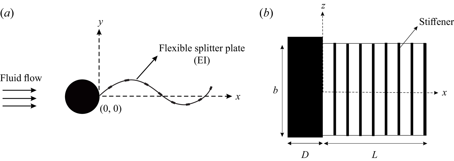
Figure 1. Schematic of a flexible splitter plate/flap in the wake of a circular cylinder: (a) top view; (b) side view. In the figure, the flexible splitter plate/flap of length  $L$, and flexural rigidity $EI$ is placed downstream of the cylinder of diameter $D$.
$D$.
In the present case, we extensively investigate two specific flap lengths ( $L$), one corresponding to $L/D=5$ and the other with $L/D=2$. In the $L/D=5$ flap case, the flap length is sufficiently long that for large $EI$ values it approaches a long rigid plate case, which is known to suppress vortex shedding. On the other hand, for the $L/D=2$ flap case, even the rigid plate is not expected to suppress shedding. We show that the observed flap dynamics for the two length cases can be dramatically different. In both length cases, at large values of $EI$, the configuration approaches that of a rigid splitter plate, while at very low values of $EI$, the effects of the flexible splitter plate would be expected to be small. On the other hand, one might expect that at intermediate values of the flexural rigidity, there would be significant interactions between the elastic deformations of the flap, the fluid forces acting on the flap and the wake dynamics. We have experimentally studied this in the present work through measurements of the flap deformations, forces and the wake dynamics.
In § 3, we discuss results for the  $L/D=5$ cases. This includes the effect of the flap's flexural rigidity ( $EI$) on its dynamics, the fluctuating lift and mean drag forces acting on the body and the wake dynamics obtained from particle image velocimetry (PIV) measurements. This is followed in § 4 by a similar discussion about $L/D=2$ cases, where the length of the flap is less than or equal to the recirculation zone. The main conclusions from the study are presented in § 5.
2. Experimental details
The main part of the work presented in this paper was performed in a free surface water tunnel in the fluid mechanics laboratory of the mechanical engineering department at the Indian Institute of Science (IISc). The test section of the tunnel is  $1\ {\rm m}\times 1\ {\rm m}$ in cross section and 3 m long. The tunnel is a closed circuit type with contraction ratio of 7.50. The maximum speed of the tunnel is 1 m s $^{-1}$. The test section frame is made of mild steel with six glass panels on the side walls and three Perspex panels on the floor, and the maximum height of the water level in the test section is 1 m from the base of the test section.
A Pitot static probe in conjunction with a two-liquid manometer was used for measuring the flow speed in the test section. The two liquid manometer contained two liquids with a density ratio of  ${ \rho _{l} }/{ \rho _{w} } = 1.12$, which provided a magnification factor of approximately 8 in the manometer reading compared with a single liquid water manometer reading ( $\Delta H$) as given by the equation
 \begin{equation} \frac{\Delta h}{\Delta H}= \frac{1}{ \dfrac{\rho_{l}}{\rho_{w}}-1}, \end{equation}
where  $\rho _l$ is the density of the manometer liquid, $\rho _w$ is the density of water in the tunnel, $\Delta h$ is the two-liquid manometer reading and $\Delta H$ is the dynamic head in the test section in terms of the equivalent water column. With this amplification factor, the two-liquid manometer provided good sensitivity to measure the mean flow. Wake velocity field measurements using PIV were done in another smaller water tunnel in the department, because of the prohibitive cost of seeding the large volume of water in the larger water tunnel. The smaller water tunnel has a test section with cross-sectional dimensions of 0.45 m (height) $\times$ 0.28 m (width) and is 1.2 m long. The tunnel is also a closed circuit type with a contraction ratio of 6. The maximum speed of this tunnel is 0.30 m s $^{-1}$. The upstream end of the contraction contains the flow straightener consisting of 250 mm long and 5 mm diameter plastic straws to improve the flow quality in the test section.
The test circular cylinder was constructed of brass. The cylinder model was carefully machined such that it could be dismantled into two semicircular halves by removing the holding screws along the span of the model. Once the two halves were assembled, the screws holes were carefully filled in with sealant material such that the surface of the cylinder was smooth. This arrangement was necessary to place the flexible splitter plates in between the two halves of the model. The diameter of the cylinder was 0.035 m and its length was 0.43 m, giving a cylinder aspect ratio (length/diameter) of 8.5. The blockage of the model in the larger tunnel was 3.5 % and in the smaller tunnel was 11.7 %. To encourage two-dimensional vortex shedding, end plates were used for all the measurements presented in this thesis. The end plates were made of Perspex sheet of thickness 1 mm. The length of the end plate along the streamwise direction was  $10D$ and the width of the plate across the flow direction was $6D$ ( $D$ is the cylinder diameter), which was sufficient to cover the full length and oscillatory motion of the flexible plate.
2.1. Flexible splitter plate
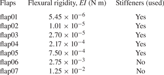
The flexible splitter plates or flaps were made from sheets of different elastic materials and thicknesses procured from stationery shops. This enabled us to get a very large range of flexural rigidities ( $EI$) for the flaps, which were measured from simple static deflection tests of the flap under its own self weight. With knowledge of the geometry, careful weighing of the flap to obtain mass per unit length and the tip deflection, the flexural rigidity per unit span of these flaps were calculated as tabulated in table 1 for each of the 7 flaps used. As seen in the table, the $EI$ values of the flaps spanned about 4 orders in magnitude. The flap aspect ratio, defined as the flap streamwise length ( $L$) to the flap width ( $b$), was 1.7 and 4.25 for the $L/D=5$ and $L/D=2$ flap cases, respectively. Initial tests showed that the motion of the flap had spanwise variations for low flexural rigidity ( $EI$) flaps. In order to achieve two-dimensional motions of the flap, we used spanwise stiffeners to locally enhance the spanwise stiffness of the flaps (Shelley, Vandenberghe & Zhang Reference Shelley, Vandenberghe and Zhang2005), as shown in figure 1. The stiffeners were made from relatively rigid elastic material with thickness of approximately 450 $\mathrm {\mu }$m. These stiffeners were carefully cut out with the help of a sharp knife and glued on both sides of the flaps at regular streamwise intervals. The stiffener streamwise size (width) and number were chosen in such a manner as to keep the width of the stiffeners to be small compared with the streamwise wavelength of the plate deformations, and the separation between two successive stiffeners to be large enough compared with the stiffener width, to not affect the flexural rigidity ( $EI$) of the base flap in the streamwise direction. This resulted in 10 stiffeners being used for the $L/D=5$ case and 4 stiffeners for the $L/D=2$ case. It was also ensured that the stiffener streamwise width was kept small compared with the streamwise wavelength of the plate deformations to again ensure that there was no effect on $EI$ of the base flap. It may be noted that stiffeners were used only for flaps whose flexural rigidity was low (flap01 to flap05) to keep the deformations two-dimensional, while no stiffeners were used in the higher $EI$ flap cases, as indicated in table 1. The flap deformations in all flap cases presented were ensured to be two-dimensional. Flap tip amplitudes and deformation profiles in both with and without stiffener cases were seen to be close as indicated by the collapse of the tip amplitude values for flap05 (with stiffener) and flap07 (without stiffener) when plotted with non-dimensional stiffness parameter, $K^{\ast }$, as shown in figure 6.
Table 1. Measured flexural rigidity  $EI$ per unit span of the different flexible splitter plate/flaps that were used in the present investigation.
2.2. Measurements
Flap dynamics were captured using a Fastcam PCI R2 camera in conjunction with a Roithner 1 W continuous green (532 nm) laser. The laser sheet was generated using a 7 mm cylindrical lens and illuminated a viewing area with a streamwise length of about  $9D$. The camera framing rates were chosen according to the oscillation frequency of the plate, which was dependent on the flow speed. The maximum framing rate used was 250 frames/second, which was sufficient to capture at least 40 images per cycle of the plate/flap motion at the highest flow speed, with significantly higher images per cycle being captured at lower flow speeds.
In all cases, recorded images of the flap motions were processed in MATLAB to determine tip deflection at each time instant. From the resulting time traces of tip deflection, the amplitude and frequency of flap motions were deduced. Throughout the paper, the normalised amplitude of the tip oscillations is defined as  $A^{\ast } = \sqrt {2} {Y'_{rms}/D}$, where $Y'_{rms}$ is the root-mean-square (r.m.s.) of the fluctuating part of the transverse tip deflection. The normalised frequency of tip oscillations is defined as $f_{A}D/U$, where $f_{A}$ is the flapping frequency of the flap that is obtained from the spectra of the time traces of tip deflection. Force measurements were carried out using a load cell attached to the top end of the cylinder and can be seen in figure 2. The load cell used had a strain-gauge-based sensing element connected to a Wheatstone bridge. The load cell directly measured the hydrodynamic forces acting on the cylinder–splitter plate configuration when it was exposed to the flow. The output voltage from the Wheatstone bridge was amplified and conditioned before acquisition. Prior to measurements, the load cell was calibrated with standard weights, and had a calibration constant of 50.2 mV/gram-force (gm-f) with an uncertainty of $\pm 0.16$ mV (gm-f) $^{-1}$ based on the calibration data. This represents an error of approximately 0.3 % in the reported values of force due to calibration issues. The data acquisition of the load cell signal after signal conditioning was done using a NI Compact Data Acquisition-Model 1974 ( $NIcDAQ-1974$).
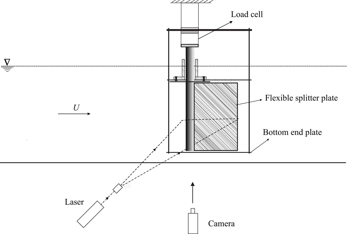
Figure 2. Schematic of the visualisation system used for PIV measurements and for recording of the flap dynamics along with experimental set-up showing the major components of the system.
Particle image velocimetry was used to measure the wake velocity field. For this technique, the flow was seeded with silver-coated spherical hollow glass particles (SH400S33) of 14  $\mathrm {\mu }$ mean diameter from Potters Industries, USA, whose density was 1.7 g cm $^{-1}$. The images of these particle were recorded using a two-dimensional PIV system after illumination by laser sheet from a New Wave Solo Nd:YAG PIV laser; a schematic of the visualisation system is given in figure 2. Pairs of such images recorded with small time intervals of the order of a few milliseconds were processed using DynamicStudio software from Dantec Inc., and a revised version of the MATLAB-based PIV code whose details are given in Govardhan & Williamson (Reference Govardhan and Williamson2000). The processing resulted in a velocity field over the entire region of imaging. The field of view used had a width of $6D$ to $8D$ for the PIV measurements reported here. This was found to give sufficient resolution of the vortical structures in the wake, while also giving a reasonable overview of the wake dynamics. A Dantec PIV camera with a resolution of $1360\ {\rm pixel}\times 1036\ {\rm pixel}$ was used to acquire particle images. The camera and laser were synchronised by providing appropriate delay time between the laser pulses (L1 and L2) and the camera using a Stanford Delay Generator (DG 645). The separation times ( $\Delta t$) between the two laser pulses (L1 and L2) was in the range of 2–15 ms, which were selected according to the flow speed in such a way that it would give about 6 pixel displacement at each speed (for the uniform flow).
Phase-averaged PIV measurements were done for all the periodic modes found in the present work to elucidate the repeatable large-scale coherent vortical structures in the flow. The PIV images for the phase averaging at a particular phase were chosen by ensuring that the variations in flap tip deflections and flap deflection profile were within 5 % of the chosen value at a given phase of flap deformation. The phase was determined based on the flap tip position with reference to the extreme location of the flap tip during the oscillation cycle. These chosen PIV images were then processed, with at least 10 such conditional velocity fields being averaged to obtain each of the phase-averaged velocity fields presented in this paper. The resultant phase-averaged fields for the  $L/D=5$ and $L/D=2$ cases are shown in §§ 3 and 4, respectively.
3. Flexible splitter plate with  $L/D=5$

In this section, we report results for a flexible splitter plate/flap with a flap length to cylinder diameter ratio  $L/D$ of 5.0. As discussed in the introduction, a rigid flap of this length would completely suppress vortex shedding from the body. In our case, the flexible plate or flap is attached to the base of the cylinder and is free to deform continuously along the length of the flap. The hinged–rigid splitter plate case with this length (Shukla et al. Reference Shukla, Govardhan and Arakeri2009), discussed in the introduction, showed only weak aperiodic oscillations as only weak interaction was possible between the shear layer on either side of the cylinder in that configuration. In contrast, in the present work with a flexible flap, local pressure communication is possible at every streamwise location along the flap length/surface, which can lead to local deformations of the plate/flap. Hence, one can expect relatively more complex deformations than in the hinged–rigid splitter plate case.
We present results for a flexible flap in the wake of a circular cylinder in three subsections. In the first subsection, we discuss the flap kinematics including the effect of the flow speed and the flap's flexural rigidity  $EI$ on it, and the combination of the flow speed and $EI$ effect into a single normalised stiffness parameter, $K^{\ast }$, of the cylinder–flap combination. The force measurements are subsequently presented in the second subsection, with the corresponding wake velocity fields from PIV measurements being presented in the final subsection.
3.1. Flap kinematics
The flap visualisations in figure 3 show a time sequence of eight images in a cycle for two sample cases with  $EI$ and $Re$ values as given in the caption. The eight images in the figure are separated by one-eighth of the oscillation period ( $T$). It may be noted that the two cases shown in figures 3(a) and 3(b) correspond to mode I and mode II response, respectively, as discussed later with reference to the amplitude response plot of the type shown in figure 4. The time sequence in figure 3(b) shows large-amplitude periodic oscillations of the flap with tip amplitudes of the order of one cylinder diameter. In the first image of this sequence ( $t=0$) corresponding to mode II, a local maximum deflection can be seen just downstream of the cylinder. As time progresses, this local maximum is seen to move to the right and one can follow the peak as it travels along the flap, and reaches close to the tip of the flap at $t=7T/8$. At this time, one can see the formation of a new local maximum again close to the cylinder, which travels downstream, and the cycle repeats. One can equivalently also see a peak on the lower side travel along the flap, with the cycle repeating. This clearly suggests that the deformations of the flap in mode II are in the form of a travelling wave, and a simple model for this is discussed later in this subsection. In the case of mode I shown in figure 3(a), a similar travelling-wave pattern of flap deformation may be seen, although the amplitudes are smaller than in mode II in figure 3(b). Superposed images of the flap deformations in the two cases are shown in figures 3(c) and 3(d), respectively, with these images showing that the amplitude of the travelling wave grows almost linearly with streamwise distance in both the cases. Further, the trajectory of the flap tip in both cases is shown in figures 3(e) and 3(f), respectively, and one can clearly see the figure-of-eight shapes traced out by the flap tips in both cases, with the same of rotation being the same in both cases. A closer look at the figure of eight in the two cases shows some differences in its streamwise orientation, which we show to be related to the phase of the streamwise flap tip oscillations relative to the transverse motions that will be shown to drastically change the vortex formation in the two cases. Also shown in figures 3(g) and 3(h) are two non-periodic asymmetric modes that we refer to as modes A1 and A2, which are seen with higher flap flexural rigidities and at lower flow speeds. In the case of mode A1, the flap deformation continues to be in the form of a travelling wave and the asymmetry about the mean line is clear about 1 $D$ downstream of the cylinder base. On the other hand, in the case of mode A2, the flap deformation is in the shape of the first bending mode of the flap, and the asymmetry about the mean line is clear at the flap tip location.
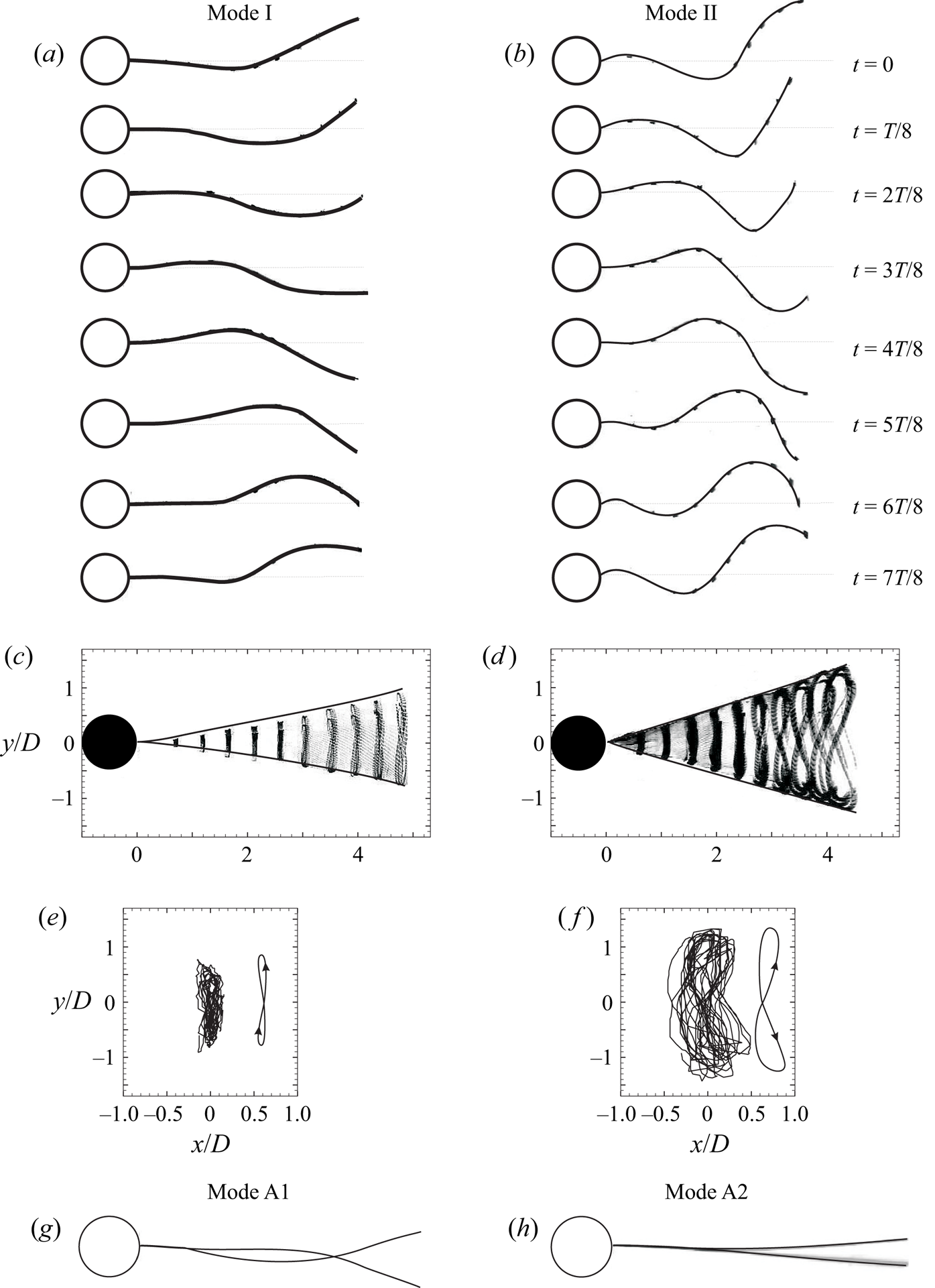
Figure 3. Time sequence of pictures showing the deformation shapes of flap over one oscillation cycle for mode I (a) and mode II (b). Each of the pictures shown in (a) and (b) are separated by one-eighth of the oscillation period,  $T$. The superimposed images and tip trajectories of these modes are shown in (c) and (e) for mode I and in (d) and (f) for mode II, respectively. The non-periodic and asymmetric modes A1 and A2 are shown in (g) and (h), respectively. Parameters: (a,c,e) $EI = 7.50\times 10^{-4}$ N m, $Re\approx 1.43\times 10^{4}$, $K^{\ast } = 1.40\times 10^{-3}$; (b,d,f) $EI = 5.45\times 10^{-6}$ N m, $Re\approx 1.35\times 10^{4}$, $K^{\ast } = 1.1\times 10^{-5}$; (g) $Re = 9552$, $EI = 7.50\times 10^{-4}$ N m, $K^{\ast } = 2.9\times 10^{-3}$; (h) $Re = 9090$, $EI = 1.25\times 10^{-2}$ N m, $K^{\ast } = 5.0\times 10^{-2}$. Supplementary movies 1 and 2 (available at https://doi.org/10.1017/jfm.2023.755) show the temporal behaviour of flap deformations corresponding to mode II and mode I oscillations, respectively.
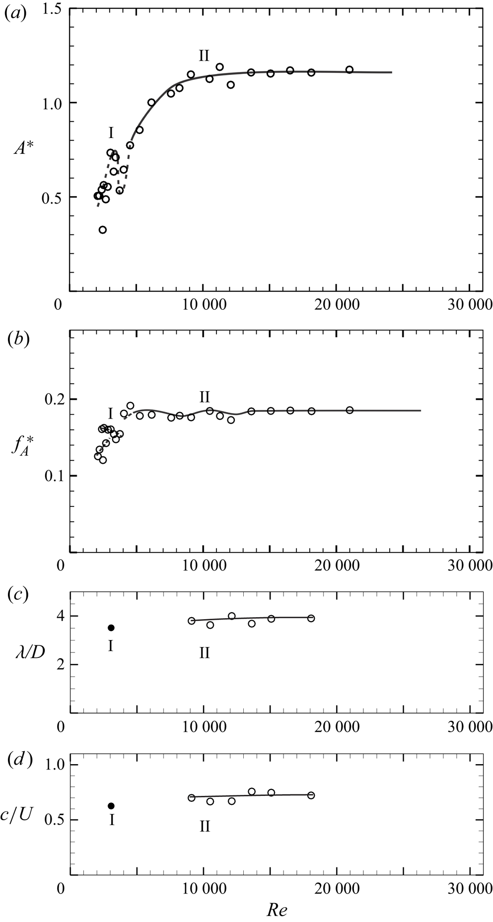
Figure 4. (a) Amplitude, (b) frequency, (c) wavelength and (d) phase speed of the thin  $L/D = 5$ flexible splitter plate/flap motion with $Re$. The two periodic flap deformation modes on the plot are marked as mode I and mode II. In (a) and (b), regions with aperiodic flap motions are indicated by dashed lines, whereas periodic flap motions are indicated by solid lines. Wavelength and phase-speed data in (c) and (d) are shown only for the periodic flap motions. Here $EI = 5.45\times 10^{-6}$ N m.
The observed shapes of the flap are indicative of the unsteady pressure field on the flap surface due to the shed vortices from the cylinder. As these shed vortices convect downstream along the flap, the flaps deform depending on the streamwise location of the shed vortex, with the travelling wave speed likely being decided by the convection speed of the shed vortices. We shall later present the corresponding vorticity fields to highlight this point. On a more general note, the observed deformation shapes of the flap seen here are reminiscent of the undulating shapes of a fluttering flag that have been studied by Connell & Yue (Reference Connell and Yue2007) and Eloy et al. (Reference Eloy, Kofman and Schouveiler2012) with the deformation shapes in both cases being in the form of a travelling wave.
Although there are variations in the deformation shapes with flow speed and flexural rigidity ( $EI$), as shown in figures 3(a) and 3(b), the deformations are in general in the form of a travelling wave except for the non-periodic mode A2. The simplest model of a travelling wave with a single frequency is one whose frequency/wavelength does not change as the wave propagates. In this case, the deflection ( $Y_{x}$) at any streamwise location ( $x$) can be written as
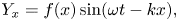 \begin{equation} Y_{x} = f(x) \sin (\omega t-kx), \end{equation}
where  $f(x)$ is the amplitude variation with $x$,
$x$,  $\omega$ is the angular oscillation frequency and $k =2\pi /\lambda$ is the wave number associated with the disturbance of wavelength $\lambda$.
The amplitude variation ( $\,f(x)$) with streamwise distance ( $x$) may be obtained from visualised images of the flaps as shown in figure 3(c), which suggests that amplitude increases almost linearly with $x$. Hence, a simple linear amplitude model is used with zero amplitude at the base of the cylinder and increasing linearly to a maximum value of $A$ at the tip: $f(x) = (A/L) x$, where $A$ is the transverse measured flap tip amplitude from the flap visualisations. The phase speed ( $c = \omega / k$) and wavelength associated with the travelling wave model can also be estimated directly by using the recorded images. The phase speed was obtained from the streamwise location of the node of the flap at successive times, and was found to be about $0.8U$ (where $U$ is the free-stream velocity) with some variation with flow speed. The wavelength ( $\lambda$) was measured directly as the distance between the streamwise location of successive wave amplitude peaks and was found to be about $4D$. The measured $c$ and $\lambda$ values are broadly consistent with the speed and spacing of shed vortices from a bare cylinder, which may be expected for a very thin flap with very small values of flexural rigidity $EI$, as in this case. The variation of the normalised wave length ( $\lambda /D$) and phase speed ( $c/U$) at different $Re$ is shown in figures 4(c) and 4(d), respectively.
The variation of the normalised tip amplitude and frequency of the flap with  $Re$ is shown in figure 4(a,b), for the case of the flap shown in figure 3(b). In the figure, the normalised flapping amplitude ( $A^{\ast } = (\sqrt {2}Y'_{rms}/D)$) and frequency ( $\,f^{\ast }_{A} = f_{A}D/U$) of the flap have been defined using the r.m.s. flap tip deflection, and the dominant frequency of the flap tip oscillation, as discussed in § 2. The amplitude response of the flap resembles that of a tethered sphere (Govardhan & Williamson Reference Govardhan and Williamson2005), with the presence of a local peak in amplitude response at $Re \approx 2500$ followed by a decrease and an eventual rise of the amplitudes ( $A^{\ast }$) to a saturated level of about 1.1. As in the tethered sphere case, we refer to the local peak in amplitude response as mode I and the higher saturated amplitude as mode II, and we shall see the differences between these two modes, apart from the amplitude, in the oscillation frequency, the forces and in the wake velocity fields.
The mode I oscillations occur at the local peak in the amplitude response where the motion of the flap is very regular. On either side of it, at higher and lower flow speed or  $Re$, the motions of the flap are aperiodic, and the corresponding long time averaged flap tip amplitudes, defined here in terms of the r.m.s. flap tip deflection are smaller, and the spectra are also broad band. In the figure the aperiodic oscillations are shown in dashed line, whereas the periodic oscillations are indicated by a solid line. At lowest $EI$ values, as in this case, the periodic mode I occurs only in a narrow regime of the local peak in amplitude marked as mode I. The periodic mode II of the flap oscillation occurs in this case for $Re > 9000$, and exhibits a saturated maximum amplitude ( $A^{\ast } \approx 1.1$) and frequency ( $\,f^{\ast } \approx 0.19$). The normalised wavelength ( $\lambda /D$) and phase speed ( $c/U$) of the propagating wave along the length of the flap for mode I are both a little lower in magnitude compared with that for periodic mode II, where these quantities of wave propagation become almost saturated and appear to be unaffected by flow speed or $Re$. It should be noted that the normalised phase speed ( $c/U \approx 0.8$) in mode II is very close to the convection speed of shed vortices in the cylinder wake without flap. The non-periodic modes A1 and A2 occur at lower flow speeds and are not clear in this flap case. They will be seen clearly in the other (stiffer) flap cases shown in figures 5 and 6.
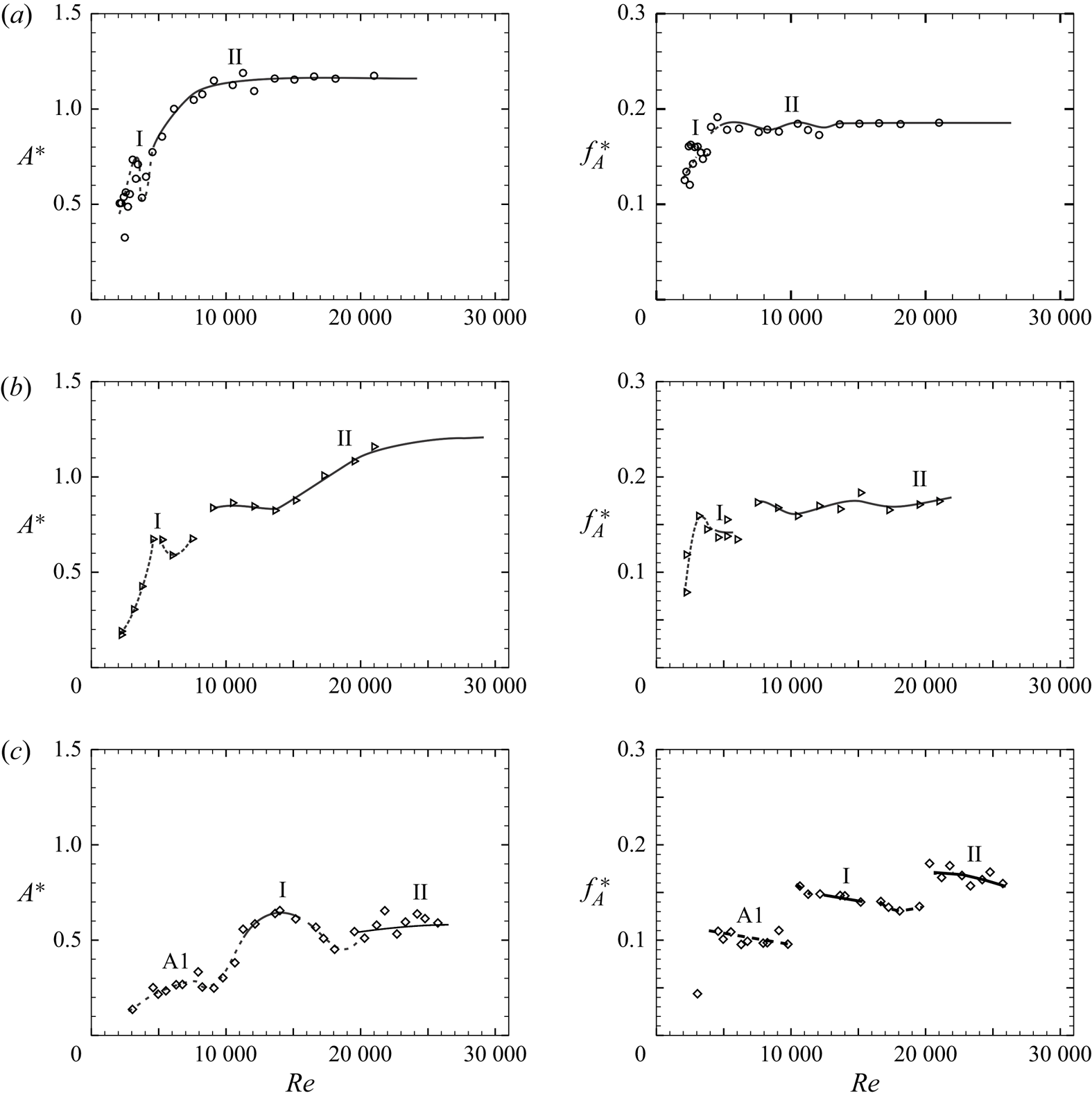
Figure 5. Amplitude (left column) and frequency (right column) response of the flap tip oscillation with  $Re$ for different flexural rigidity ( $EI$) flaps: (a) $EI = 5.45\times 10^{-6}$ N m ( $\circ$); (b) $EI = 2.70\times 10^{-5}$ N m ( $\triangleright$); (c) $EI = 7.50\times 10^{-4}$ N m ( $\diamondsuit$). Each of the plots shows the response at a particular $EI$, with the $EI$ value increasing from (a) to (c). The periodic modes I and II of the response plots appear to occur at higher $Re$ as $EI$ of the flap increases. The non-periodic mode A1 is seen for the stiffer flap in (c) at lower $Re$.
$Re$.
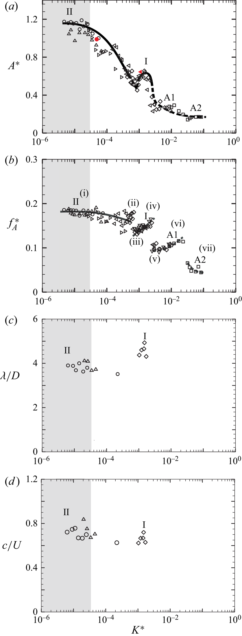
Figure 6. (a) Amplitude, (b) frequency response of the flap tip deflection with the non-dimensional stiffness,  $K^{\ast }$ for $Re > 5000$. The corresponding wavelength and phase speed of the flap deformations is shown in (c) and (d), respectively. Solid and dashed lines in the plots have the same meaning as in figure 4. In (a), all the open data symbols shown are from the bigger tunnel, whereas the solid red symbols correspond to the data from the smaller tunnel used for PIV measurements: $\circ$, $EI = 5.45\times 10^{-6}$ N m; $\triangle$, $EI = 1.01\times 10^{-5}$ N m; $\triangleright$, $EI = 2.70\times 10^{-5}$ N m; $\triangleleft$, $EI = 2.17\times 10^{-4}$ N m; $\diamondsuit$, $EI = 7.50\times 10^{-4}$ N m; $\square$, $EI = 1.25\times 10^{-2}$ N m.
In figure 5, we present the tip amplitude (left column) and frequency (right column) data as a function of  $Re$ for different values of flexural rigidity ( $EI$), with $EI$ increasing from (a) to (c). In each case, the local peak in amplitude at lower $Re$ is marked as (mode) I and the periodic regime at higher $Re$ as (mode) II, with the similar notation also shown in the frequency response. In the stiff flap in figure 5(c), one can also see the emergence of the non-periodic mode A1 at lower $Re$. It is clear from these response plots that as the flexural rigidity or $EI$ of the flaps is increased, the two periodic modes, one corresponding to local peak in $A^{\ast }$ or mode I, and the other corresponding to the saturated amplitude and frequency, or mode II, shift to higher $Re$, indicating that larger flow speeds are required to get the same mode of response. This suggests that there is a better non-dimensional parameter to characterise the effect of flexural rigidity ( $EI$) of the flap, as discussed in the following. In VIV studies of elastically mounted bodies, a non-dimensional velocity, $U^{\ast }=U/(f_{n}D)$ is used, where $f_{n}$ is the natural frequency based on the stiffness ( $k$) of the spring and the inertia ( $m$) of the moving mass. In the present case of a thin elastic flap, its natural frequency is the same as the natural frequency of an elastic cantilevered beam and is given as $f_{n} = (a_{n}/(2\pi L^{2}))\sqrt {{EI}/{m_{L}}}$, where $EI$ is the flexural rigidity (N m) of the flap per unit span length, $a_{n}$ is a constant that is dependent on the mode shape and $m_{L}$ is the mass of the vibrating flap per unit streamwise length (and per unit span length), which should also include the fluid added mass. Since in the present work the mass of the flap is very low compared with the added mass or inertia, as mentioned in the introduction, the mass of the flap is not considered as a parameter for the investigation. Thus, the natural frequency of the flap in the present problem depends upon the mode of oscillation and added inertia of the fluid flow. Hence, this type of natural-frequency-based parameter is not convenient, as although the flexural rigidity of the flap is clear, the relevant inertia is not a priori well defined. Thus, a better parameter here would be a non-dimensional bending stiffness of the flap ( $K^{\ast }$), which may be defined as in Shukla et al. (Reference Shukla, Govardhan and Arakeri2013) as
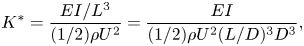 \begin{equation} K^{{\ast}} =
\frac{EI/L^{3}}{(1/2)\rho U^{2}} = \frac{EI}{(1/2) \rho U^{2}
(L/D)^{3} D^{3}}, \end{equation}
\begin{equation} K^{{\ast}} =
\frac{EI/L^{3}}{(1/2)\rho U^{2}} = \frac{EI}{(1/2) \rho U^{2}
(L/D)^{3} D^{3}}, \end{equation}
where  $EI/L^{3}$ is the stiffness (per unit span) and $(1/2)\rho U^{2}$ is the dynamic pressure ( $\rho$ is the density of the fluid, $U$ is the free-stream velocity). This non-dimensional stiffness is similar to the relative bending rigidity of the flap as defined in the flag flutter problem (Argentina & Mahadevan Reference Argentina and Mahadevan2005; Connell & Yue Reference Connell and Yue2007).
Figure 6 shows amplitude (a) and frequency (b) response of the flap with non-dimensional stiffness  $K^{\ast }$ for $Re > 5000$, respectively. All amplitude and frequency data of the response plots in figure 6 ( $Re > 5000$) appear to collapse well and demonstrate a trend shown by the combination of solid and dashed line, with the solid line indicating periodic motions and the dashed line representing aperiodic motions, as shown in figure 7. On the other hand, response data for $Re <5000$ are scattered from the higher $Re$ trend, and do not collapse when plotted with $K^{\ast }$ as shown in figure 8. In this case, we choose to show the trend line for the $Re > 5000$ data along with the $Re < 5000$ data to highlight the differences in the $Re < 5000$ data from the other set.
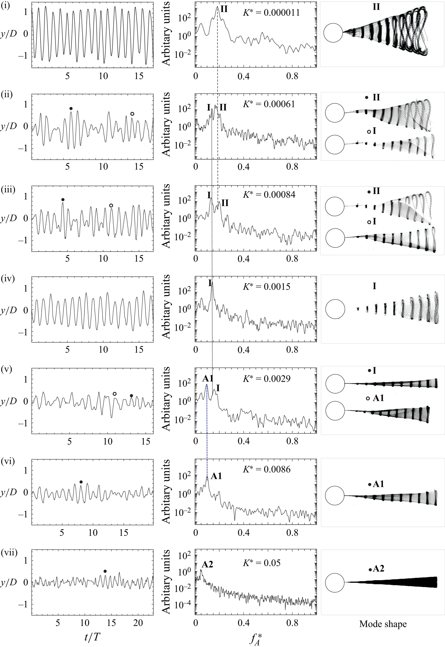
Figure 7. Transition between modes as  $K^{\ast }$ is increased for $Re>5000$. At each $K^{\ast }$, the figure shows flap tip time traces, spectra and mode shape corresponding to the dominant (one or two) frequencies. The corresponding points in the response are marked in figure 6 as (i) to (vii): (i) $K^{\ast } = 1.1\times 10^{-5}$; (ii) $K^{\ast } = 6.1\times 10^{-4}$; (iii) $K^{\ast } = 8.4\times 10^{-4}$; (iv) $K^{\ast } = 1.5\times 10^{-3}$; (v) $K^{\ast } = 2.9\times 10^{-3}$; (vi) $K^{\ast } = 8.6\times 10^{-3}$; (vii) $K^{\ast } = 5\times 10^{-2}$.

Figure 8. (a) Amplitude and (b) frequency response plots of the flaps with the non-dimensional bending stiffness,  $K^{\ast }$, for $Re < 5000$. Lines shown in plots are trend lines of the response for $Re > 5000$: $\circ$, $EI = 5.45\times 10^{-6}$ N m; $\triangle$, $EI = 1.01\times 10^{-5}$ N m; $\triangleright$, $EI = 2.70\times 10^{-5}$ N m; $\triangleleft$, $EI = 2.17\times 10^{-4}$ N m; $\diamondsuit$, $EI = 7.50\times 10^{-4}$ N m; $\square$, $EI = 1.25\times 10^{-2}$ N m.
It is therefore clear that there is a distinct difference between the two data sets. The difference appears to be related to the large reduction in fluctuating lift for a bare cylinder in the  $Re$ range between about 1600 and 5000 discussed by Norberg (Reference Norberg2003). This drop is likely related to changes in the three-dimensional shedding mode at these $Re$ as discussed in Prasad & Williamson (Reference Prasad and Williamson1997). We shall henceforth, for sake of clarity, concentrate mainly on $Re > 5000$ data, where all the amplitude response data is well collapsed by the non-dimensional stiffness $K^{\ast }$ independent of $Re$. From the collapsed data in figure 6 for $Re > 5000$, one can see that the periodic mode I oscillations occur at $K^{\ast } \approx 1.5\times 10^{-3}$, while the periodic mode II response occur at very low $K^{\ast }$ ( $\approx \leq 3.0\times 10^{-5}$). Although the low $K^{\ast }$ data corresponding to the saturated mode II are seen to collapse well, a closer look shows that the amplitude data shows some variations, from about 1 to 1.2 depending on the flap's stiffness. This is likely related to a weak $Re$ effect as seen for example in the case of VIVs of a cylinder in Govardhan & Williamson (Reference Govardhan and Williamson2006), where the amplitude varied logarithmically with $Re$. It should be emphasised here that while there is a band of amplitudes at a given $K^*$ value related to a possible weak $Re$ effect, the overall collapse, in terms of $K^*$, for example, in the range of $K^*$ values where mode II or mode I is seen, does seem to collapse well independent of $Re$, as long as $Re>5000$, as shown in figure 6. At high $K^{\ast }\approx 1\times 10^{-2}$, the non-periodic and asymmetric mode A1 can be seen, while the other non-periodic mode A2, is seen at even higher $K^{\ast } \approx 5\times 10^{-2}$, the latter having deformations in the form of the first bending mode. The corresponding variations of the wavelength and phase speed of the plate deformations with $K^{\ast }$ are shown in figures 4(c) and 4(d), respectively. Figure 6(d) shows that there is a reduction in the phase speed from values of approximately $0.8U$ to $0.7U$ as $K^*$ (and flexural rigidity) is increased from values corresponding to mode II to higher $K^*$ values corresponding to mode I. The variations of both phase speed and wavelength while significant (about 15 to 20 %) within this range are not too large. This may be attributed to the very low plate mass ratios ( $m^*$) used in the present experiments, which implies that the fluid added mass dominates over structural mass, resulting in a strong coupling of the fluid and the structure. At $K^*$ values higher than at mode I, periodic oscillations are not seen, and hence phase speed and wavelength data are not shown in these cases.
As  $K^*$ is increased from very low values, the flap dynamics transitions from one mode to the other. These transitions and the resulting competition between modes is illustrated in figure 7, which shows, at a few different $K^*$ values (marked in figure 6 as (i) to (vii)), the plate tip time traces, its long-time averaged spectra and mode shapes corresponding to the dominant (one or two) frequencies. In (i), at low $K^*$ values, periodic plate tip deformations can be seen with a single dominant frequency corresponding to mode II oscillations as shown by the superposed plate deformation profile. At higher $K^*$ values (in (ii)), one can see the existence of two frequencies, the higher one corresponding to mode II type oscillations, while the lower one corresponds to mode I type oscillations, with mode II type having larger relative streamwise oscillations as seen earlier. The flapping mode shape in cases with two frequencies as in (ii) are superposed only over a single cycle that is identified on the time trace by $\circ$ and $\bullet$, and the corresponding symbol is also shown with the mode shape. In (iii), at larger $K^*$ values, the two peaks in frequency continues, with mode I now becoming dominant compared to in (ii). It may be noted here that in both (ii) and (iii), the flap deflection profiles are not very periodic and show asymmetry about the mean line that is evident at about 1 $D$ downstream of the cylinder base. Subsequently, with increasing $K^*$, we see the emergence of periodic mode I oscillations in (iv). This is followed by non-periodic oscillations with mode I and A1 in (v), mainly mode A1 in (vi) and finally at higher $K^*$ values, mode A2, whose deflection profile is like the first bending mode of a cantilever. It may be noted that the large lift fluctuations discussed later occurs in this mode. These figures thus illustrate the transition and competition between modes that occur as $K^*$ is continually increased from low values.
Superposed images of the flap tip deflection corresponding to the two periodic modes are shown in figures 3( $c$) and 3( $d$) to highlight differences between the modes, as discussed briefly earlier, both cases corresponding to $Re > 5000$. Between these periodic modes, there is the obvious difference in the amplitude of tip oscillation, with mode I oscillations being smaller than that of mode II, in addition to the fact that mode II oscillations have relatively larger streamwise oscillations that are reflected as a wider figure-of-eight shape. In addition to these points, a closer look at the trajectory of the flap tip shown in figures 3( $e$) and 3( $\,f$) of also shows differences in the streamwise orientation of the figure-of-eight shape traversed by the tip in the two cases. In the mode I case (shown in figure 3 $e$), the centre of the figure-of-eight shape is displaced in the downstream direction, while it is shifted in the upstream direction in the mode II case (shown in figure 3 $f$). This is further clarified in the sketched trajectory shape for a single cycle shown on the right corresponding to both cases. This difference in the relative position of the centre of the tip trajectory may be related to changes in phase between the $x$ and $y$ motions of the flap tip, as illustrated for example in Jauvits & Williamson (Reference Jauvits and Williamson2004) for the case of two-degree-of-freedom motions of a cylinder. It should be noted here that the $x$ motions are at twice the frequency of the $y$ motions, and the phase referred to here is the phase taking this into account, i.e. $x = \sin (2\omega t + \phi$) and $y = sin (\omega t)$. Keeping this in mind, it may be noted that mode I trajectory corresponds to a phase difference $\phi = 45^{\circ }$, whereas the mode II trajectory is significantly different and corresponds to $\phi = 315^{\circ }$. These differences are an indication of larger differences that exist between these two periodic modes, and will be clarified later in this section when we present results from force and PIV measurements.
3.2. Force measurements
As discussed previously, a non-dimensional effective stiffness of the flap ( $K^{\ast }$) is a useful parameter, with the tip oscillation data for different flaps collapsing when plotted with $K^{\ast }$ for $Re>5000$. At lower $Re$ values, the data showed scatter that was attributed to a $Re$ effect. In a similar manner, we plot normalised r.m.s. fluctuating lift and mean drag force coefficients data vs the effective stiffness of the cylinder flap system ( $K^{\ast }$) respectively shown in figures 9(a) and 9(b), with this plot containing data for all flaps, but only for $Re > 5000$. The normalisation of the forces data has been done as the ratio of the respective value for the cylinder–flap system to that of the bare cylinder at the same $Re$; this being represented by $C_{l'}^{\ast }$, for the normalised fluctuating lift, and $\overline {C_{d}^{\ast }}$, for the normalised mean drag. As seen in the amplitude response plots, there is a good collapse of fluctuating lift and mean drag data across all the flaps when plotted vs $K^{\ast }$ for $Re > 5000$, as shown in figures 9(a) and 9(b), respectively. On the other hand, the data for $Re < 5000$ shows scatter which is not shown in the paper and more details can be obtained from Shukla (Reference Shukla2016), as in the tip oscillation data. It should be noted that the coefficients of r.m.s. lift and mean drag forces have been defined in the standard way as follows:
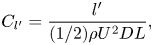 \begin{gather} C_{l'} = \frac{l'}{(1/2) \rho U^{2} D L}, \end{gather}
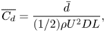 \begin{gather}\overline{C_{d}} = \frac{\bar{d}}{(1/2) \rho U^{2} D L}, \end{gather}
where  $l'$ and $\bar {d}$ represent values of the r.m.s. lift force and mean drag force of the acquired force signals, respectively. The collapsed data for the normalised fluctuating lift force coefficient ( $C_{l'}^{\ast }$) in figure 9(a) at $Re>5000$ shows interesting trends with $K^{\ast }$. At low values of $K^{\ast }$, corresponding to tip oscillations in the mode II regime as discussed in the previous section, $C_{l'}^{\ast }$ is close to about 0.6. The $C_{l'}^{\ast }$ values remain close to 0.6, as $K^{\ast }$ is increased from these low values to about $3\times 10^{-4}$. At larger $K^{\ast }$ values, a dip is seen in $C_{l'}^{\ast }$ values, with the minimum occurring at close to $K^{*} \approx 1.5\times 10^{-3}$, where we had earlier seen a local peak in the tip oscillation data corresponding to mode I oscillations. Subsequently, as $K^{\ast }$ is further increased, the lift coefficient increases rapidly reaching values of about 0.9 at $K^{\ast } \approx 0.05$, before reducing again as might be expected in the rigid splitter plate case to the far right. The peak in the $C_{l'}^{\ast }$ at $K^{\ast } \approx 0.05$ is likely related to a ‘resonant’ condition, with the natural frequency of the flap being close to the wake frequency in this case. The wake frequency corresponding to this local peak in $C_{l'}^{\ast }$ can be directly found from the spectrum of the lift fluctuations, which shows that the dominant peak occurs at a low non-dimensional frequency, $f_{l} D / U \approx 0.05$. We can also get an estimate for the non-dimensional frequency corresponding to the ‘natural frequency’ ( $\,f_{n}$) of the flexible flap. The non-dimensional form of this natural frequency ( $\,f_{n} D/U$) can be written in terms of the flexural rigidity ( $EI$) of the flap, which can in turn be expressed in terms of $K^{\ast }$ similar to the expression for reduced velocity of the plate in term of elasticity shown by Sahu et al. (Reference Sahu, Mohd and Mittal2019):
 \begin{equation} \frac{f_{n}D}{U}= (a_{n}/\sqrt{8\pi C_{m}}) \frac{\sqrt{K^{{\ast}}}}{L/D}, \end{equation}
where the constant  $a_{n}$ can be obtained from eigensolutions of the oscillating cantilever beam for a given mode of oscillation, with its value for the fundamental mode being 3.53. The constant $C_{m}$ in the equation is the added mass of the fluid and may be written as $M/(\rho L/\pi )$, where $M$ is the added mass per unit area, $\rho$ is the density of the fluid flow and $L$ is the length of the flap. This added mass parameter also depends on the mode of flap oscillation (Coene Reference Coene1992). For the fundamental mode of flap oscillation this constant is equal to $0.68\pi$ as reported by Yadykin, Tenetov & Levin (Reference Yadykin, Tenetov and Levin2002) for potential flow calculations. By using these values of constants, the non-dimensional natural frequency ( $\,f_{n}D/U$) corresponding to the fundamental mode of flap oscillation can be estimated and is found to be about 0.02. In the experiments, the flow is rotational and more complex due to the fact that it is in the wake of the cylinder. Given this difference, the non-dimensional natural frequency ( $\,f_{n}D/U$) may be closer to the wake frequency of 0.05 seen in the experiments. As we also show later, in both the $L/D=5$ and $L/D=2$ cases, the peak in lift fluctuation ( $C_{l'}^{\ast }$) appears to correspond to the case where the wake frequency is close to the structural natural frequency estimated using the stiffness and the added mass, the latter being the dominant inertia in the system. It should be noted that the flap deflection is in the form of the first bending mode in the both cases. This is illustrated in figures 20(a) and 20(b) that show a close up of the amplitude and frequency around the peak in ( $C_{l'}^{\ast }$) for the $L/D=5$ and $L/D=2$ cases, respectively. In both cases, we find that at the peak in $C_{l'}^{\ast }$, the amplitude is relatively flat locally, whereas there is a small local peak in the frequency. Although the observations in both $L/D$ cases are clear, the reasons for the increase in $C_{l'}^{\ast }$ are not clear, and needs further study. The collapsed data for the normalised mean drag force coefficient ( $\overline {C_{d}^{\ast }}$) in figure 9(b) at $Re>5000$ shows that the mean drag force continuously decreases as $K^{\ast }$ is increased. Compared with the gradual decrease in $\overline {C_{d}}$ with $K^{\ast }$, a sharp decrease in seen at $K^{\ast } \approx 1.5\times 10^{-3}$ corresponding to the mode I oscillations. After this sharp decline, the mean drag again gradually reduces with $K^{\ast }$. At large values of $K^{\ast }$, one would expect the mean drag to tend to the rigid splitter plate drag value. The non-dimensional lift force frequency ( $\,f_{l}^{*} = f_{l}D/U$) can be obtained from the fluctuating lift spectrum. Figure 10 shows the variation of $f_{l}^{*}$ with $K^{\ast }$, along with the corresponding measured frequency of the flap tip oscillation ( $\,f_{A}^{\ast }$) presented earlier from the flap kinematics data. As seen in the plot, and as may be expected, both frequencies are essentially the same at all $K^{\ast }$.
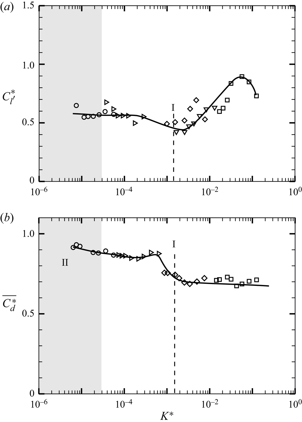
Figure 9. Plots of normalised (a) r.m.s. lift force ( $C_{l'}^{\ast }$) and (b) mean drag force coefficient ( $\overline {C_{d}^{\ast }}$) with $K^{\ast }$ for $Re > 5000$: $\circ$, $EI = 5.45\times 10^{-6}$ N m; $\triangleright$, $EI = 2.70\times 10^{-5}$ N m; $\diamondsuit$, $EI = 7.50\times 10^{-4}$ N m; $\nabla$, $EI = 2.75\times 10^{-3}$ N m; $\square$, $EI = 1.25\times 10^{-2}$ N m. In both cases, the values shown are the ratio of the force acting on the cylinder–flap system compared with the corresponding force on the bare cylinder.
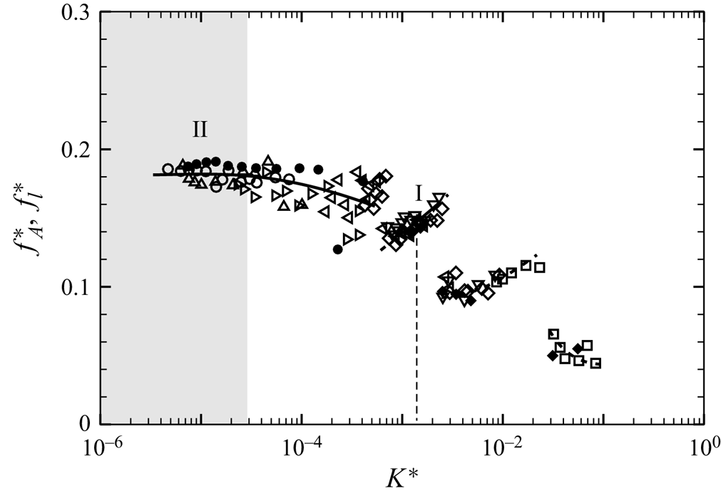
Figure 10. Plot of the variation of the non-dimensional frequencies of flap tip motion ( $\,f^{\ast }_{A}$) and fluctuating lift force ( $\,f^{\ast }_{l}$) vs the effective stiffness ( $K^{*}$). These two frequencies are very well coupled. Solid symbols show lift force frequencies ( $\,f^{\ast }_{l}$), whereas open symbols show flap tip frequencies ( $\,f^{\ast }_{A}$), with different symbols representing the different $EI$ flaps, respectively, as shown in the response plot in figure 6.
The results of the force measurements show that the fluctuating lift and mean drag of the cylinder–flap combination is mainly dependent on the effective stiffness  $K^{\ast }$ for $Re > 5000$ and found to be minimum at mode I. This is further supported by PIV measurements of wake velocity fields and turbulent stresses at mode I discussed in the next subsection. In the next subsection we examine results of the PIV measurements where we explore dynamics related to the wake vortices and results corresponding to the mean and turbulence flow fields.
3.3. PIV measurements
We now present results from PIV measurements in the wake of a cylinder with the long flexible splitter plate/flap. The variation of the wake velocity/vorticity fields as a function of the non-dimensional flexural rigidity ( $K^{*}$) of the flap is discussed through phase-averaged vorticity fields based on the flap tip location, followed by the mean flow field and the turbulence quantities. It should be noted all data presented are only for $Re > 5000$, where the results for flap kinematics and forces showed good collapse of data across different flap lengths when plotted with the effective stiffness ( $K^{*}$), and we focus our attention only on the periodic modes I and II.
The phase-averaged vorticity fields corresponding to mode II and mode I of the flap motions are shown in figure 11. The phase-averaging is done using the flap tip location as the reference, with averaging typically done over about 10 fields at nearly the same flap tip location. The phase-averaged fields corresponding to mode II (left) and mode I (right) oscillations are shown from figures 11(b) to 11(e), with a sample instantaneous bare cylinder case shown in figure 11(a) for reference. In the two flap cases, a half cycle of flap tip motion is shown starting from the first plot (in figure 11b) that corresponds to the top extreme position of the flap tip, with successive plots being spaced apart by  $T/8$, where $T$ is the time period of flap tip oscillation. In the mode II case shown in the left of the figure 11, one can see the two shear layers from the two sides of the cylinder gradually moving downstream and shed into the wake as well formed vortices after the flap tip. The non-dimensional circulation ( $\varGamma /(UD)$) of the shed vortices is about 2.55, which is reasonably close to that of the bare cylinder case shown in figure 11(a), and also the circulation value for the bare cylinder case at similar $Re$ reported by Govardhan & Williamson (Reference Govardhan and Williamson2000). In contrast, in the mode I case on the right of figure 11, the shear layers are again clearly seen closer to the cylinder, but are weaker, and they to do not form strong vortices after the flap tip. The relatively weaker vortices with non-dimensional circulation ( $\varGamma /(UD)$) of about 0.3 are responsible for the much lower turbulence intensities and shear stresses in the wake in the mode II case, as discussed a little later.
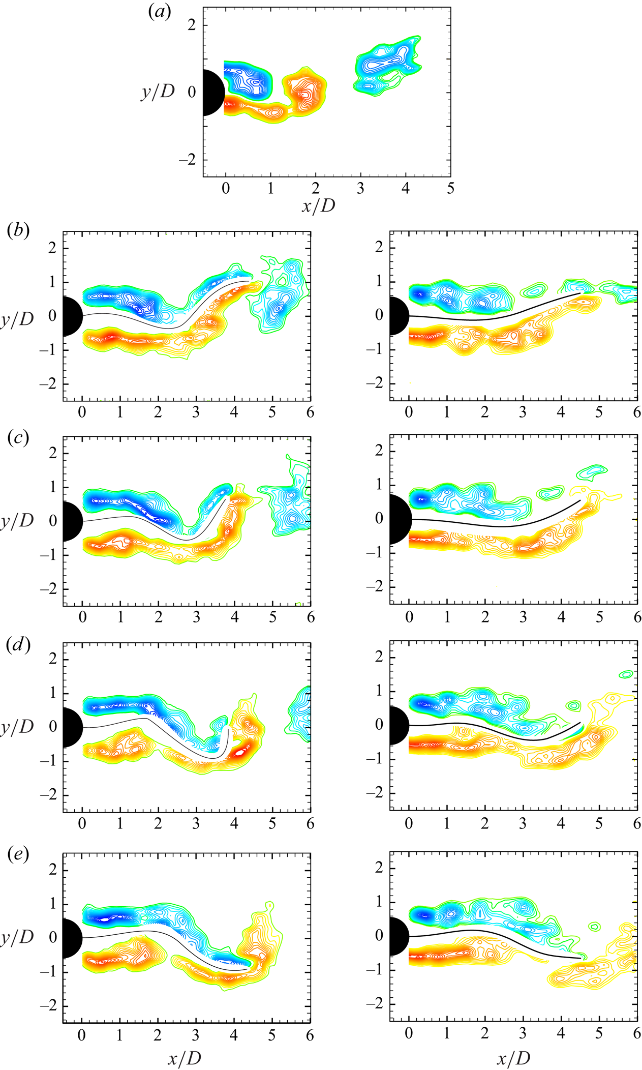
Figure 11. Phase-averaged fields corresponding to mode II (left) and mode I (right) oscillations shown in (b) to (e). The vorticity fields are phase-averaged with respect to the flap tip position. Phase-averaged fields for a half cycle of flap tip motion is shown starting from the first plot (in b) that corresponds to the top extreme position of the flap tip, with successive plots being spaced apart by  $T/8$, where $T$ is the time period of flap tip oscillation. In case of mode I, vortices that form near the flap tip are seen to be much weaker than in the mode II case. Phase-averaged vorticity fields of the reference case of the bare cylinder are shown in (a) close to the phase corresponding to the top extreme tip locations of the flaps shown in (b). Vorticity contours levels shown in all the cases are $\omega D/U = \pm 0.5, \pm 0.75, \pm 1.0, \pm 1.5,\ldots, \pm 5.0$.
Mean velocity vector fields of the cylinder wake are obtained by averaging of a large number ( $\approx$1000) of instantaneous velocity vector fields from PIV measurements. The mean streamlines and vorticity fields from these time-averaged fields at different $K^{*}$ values are shown in figure 12, all cases corresponding to a fixed $Re$ value of 8910. The four cases shown correspond to the bare cylinder, mode II, mode I and the fixed rigid splitter plate case, respectively, with $K^{*}$ progressively increasing from effectively zero for the bare cylinder case to infinity for the rigid splitter plate case. In each case, the mean streamlines are shown on the left, whereas contours of the normalised mean vorticity ( $\bar {\omega }D/U$) field are shown on the right. The dashed lines show the extreme extent of the flap's motions, whereas the solid line in the last case represents the fixed–rigid splitter plate.
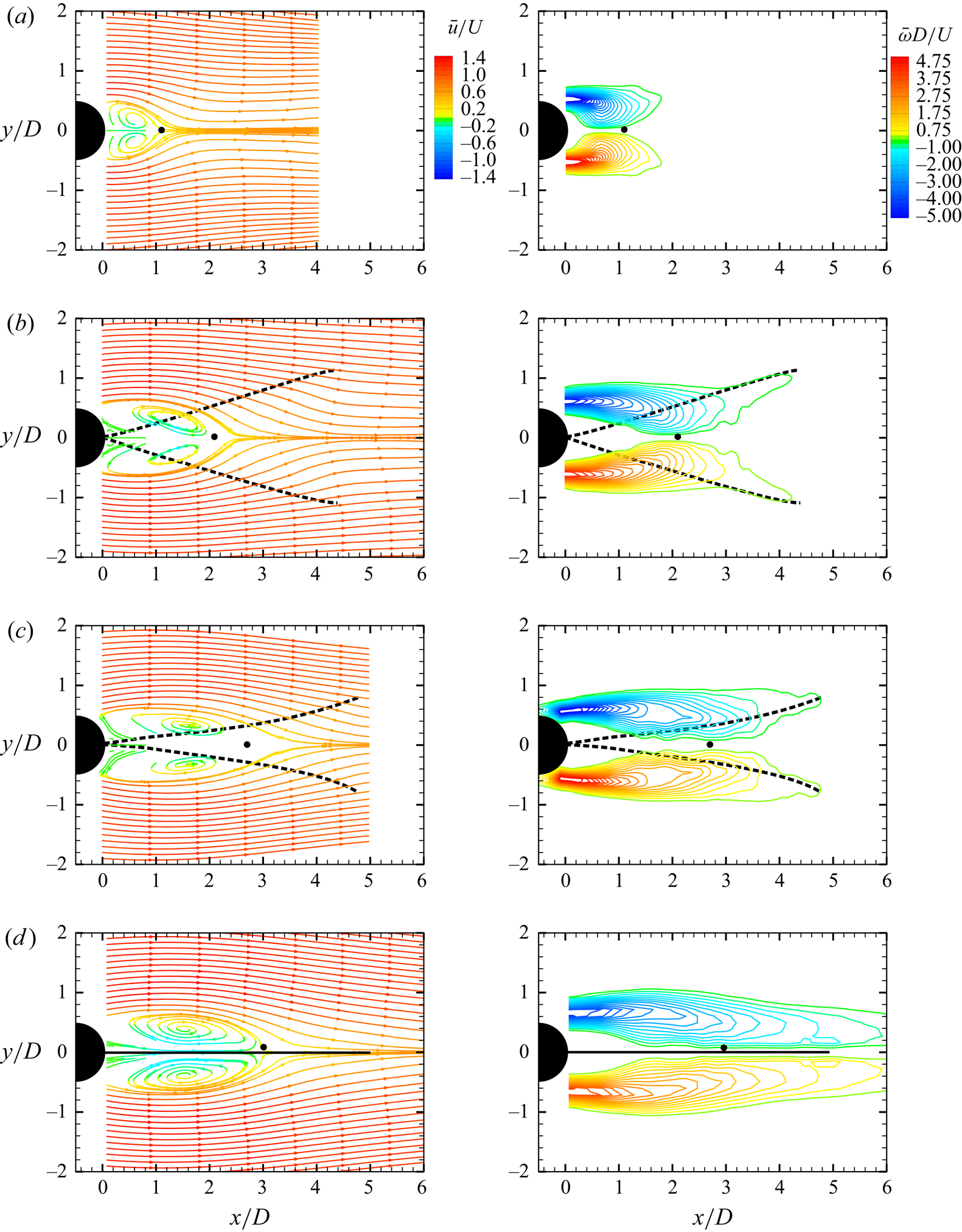
Figure 12. Mean streamlines and vorticity plots for  $Re>5000$. The plots correspond to (a) bare cylinder, (b) mode II oscillations, (c) mode I oscillations and (d) fixed–rigid plate. The Reynolds number in all cases is 8910, and the corresponding values of $K^{*}$ are (a) 0.0, (b) $4.8\times 10^{-5}$, (c) $1.1\times 10^{-3}$ and (d) $\infty$. In each case, the mean streamlines are on the left and the normalised mean vorticity contours ( $\bar {\omega }D/U$) are on the right.
From the mean velocity fields shown, the formation length ( $l_{form}/D$) can be determined, which in the present case is defined based on the closure point of the mean separation bubble. This is represented in each of the plots in figure 12 by a solid circular symbol placed on the wake centreline, and corresponds to the location of zero streamwise mean wake velocity. The distance between this closure point and the cylinder base is one of many ways of defining a formation length ( $l_{form}$) for the wake vortices. We present in table 2, the measured value of formation length from the present measurements for a bare cylinder with that of Govardhan & Williamson (Reference Govardhan and Williamson2001), also using closure point definition, at similar $Re$, to validate the measurement. As seen in the table, the values of $l_{form}/D$ in the two cases are similar.
Table 2. Comparison of the formation length ( $l_{form}/D$) for the bare cylinder based on closure point of the mean separation bubble.
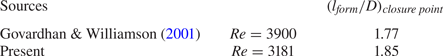
It is apparent from the mean flow fields in figure 12 that presence of the flap in the wake shifts the closure point downstream in panels (b), (c) and (d) in comparison with the bare cylinder case shown in panel (a). As  $K^{\ast }$ is progressively increased from panel (a), where it is effectively zero, to panel (d), where it is infinity, we can see a continuous downstream movement of the closure point. Even at small $K^{\ast }$ values corresponding to mode II oscillations in panel (b), one can see a substantial downstream motion of the closure point and, hence, an increase in formation length ( $l_{form}/D$). This change in formation length continuously increases as $K^{*}$ increases and becomes maximum for the limiting case of the rigid splitter plate case in panel (d). The change in formation length ( $l_{form}/D$) with $K^{*}$ is clearly shown in figure 13, which shows that it increases from about 1 for the bare cylinder case to about 2 in mode II and closer to 3 for both mode I and the rigid-splitter plate case. There is a large effect of $K^{\ast }$ on the formation length; note that all data shown are at the same $Re=8910$.
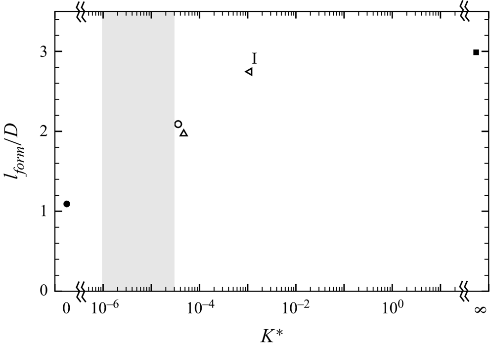
Figure 13. Variation of formation length ( $l_{form}/D$) with effective stiffness $K^{\ast }$: $\circ$, $EI = 5.45\times 10^{-6}$ N m; $\triangle$, $EI = 1.01\times 10^{-5}$ N m; $\triangleleft$, $EI = 2.17\times 10^{-4}$ N m. The plot shows that the formation length continuously increases as $K^{*}$ is increased from low values. The extreme values of $K^{\ast }=0$ corresponding to the reference case of a bare cylinder ( $\bullet$) and $K^{\ast }=\infty$ corresponding to the fixed–rigid splitter plate ( $\blacksquare$) are also shown on the plot.
The observed increase in formation length ( $l_{form}/D$) with $K^{\ast }$ may be correlated to other observed changes with $K^{\ast }$. One of the earlier observations with regard to flapping frequency ( $\,f^{\ast }_{A}$) and lift force frequency ( $\,f^{\ast }_{l}$) is their clear decrease with $K^{\ast }$, as shown in figure 10. This decrease in $f^{\ast }_{l}$ and $f^{\ast }_{A}$ with $K^{\ast }$ is essentially related to a lowering of the shedding frequency from the cylinder–flap system as the rigidity of the splitter plate is increased. Roshko (Reference Roshko1954) and Apelt et al. (Reference Apelt, West and Szewczyk1973, Reference Apelt, West and Szewczyk1975) have also linked changes in the shedding frequency to the base suction, which is, in turn, broadly a reflection of the mean drag on the cylinder. For example, Apelt et al. (Reference Apelt, West and Szewczyk1975) report changes in the shedding frequency with splitter plate length for a fixed–rigid splitter plate in the wake of a cylinder. In the present case, the shedding frequency of the wake vortices is altered by varying the effective rigidity ( $K^{*}$). As is obvious from the frequency response shown in figure 10, the flapping frequency is significantly reduced as $K^{*}$ is increased. We would expect this to lead to a decrease in base suction (Roshko Reference Roshko1954, Reference Roshko1993) and, hence, a decrease in mean drag force on the cylinder as shown in figure 9(b). An increase in formation length ( $l_{form}/D$) with $K^{*}$ is consistent with this decrease in base suction and mean drag on the cylinder.
We next present the fluctuating velocity fields in the wake of the cylinder with a flexible flap. The instantaneous data sets used for this analysis are the same as in the previous case, and comprise 4 sets of about 1000 instantaneous PIV fields. The four sets correspond, as before, to the bare cylinder, mode II and mode I oscillations, and that of the rigid splitter plate. We present contours of the streamwise velocity fluctuation ( $u'_{rms}/U$), the transverse velocity fluctuation ( ${v'_{rms}}/U$) and shear stress ( $\overline {u' v'}/U^{2}$) in figure 14 for the four cases. As before, the extent of flapping is shown by the dashed lines, whereas the fixed–rigid splitter plate is indicated by the solid line. For the bare cylinder case, a validation of the presently measured peak Reynolds shear stresses with the data of Cantwell & Coles (Reference Cantwell and Coles1983) and Govardhan & Williamson (Reference Govardhan and Williamson2001) is shown in table 3.
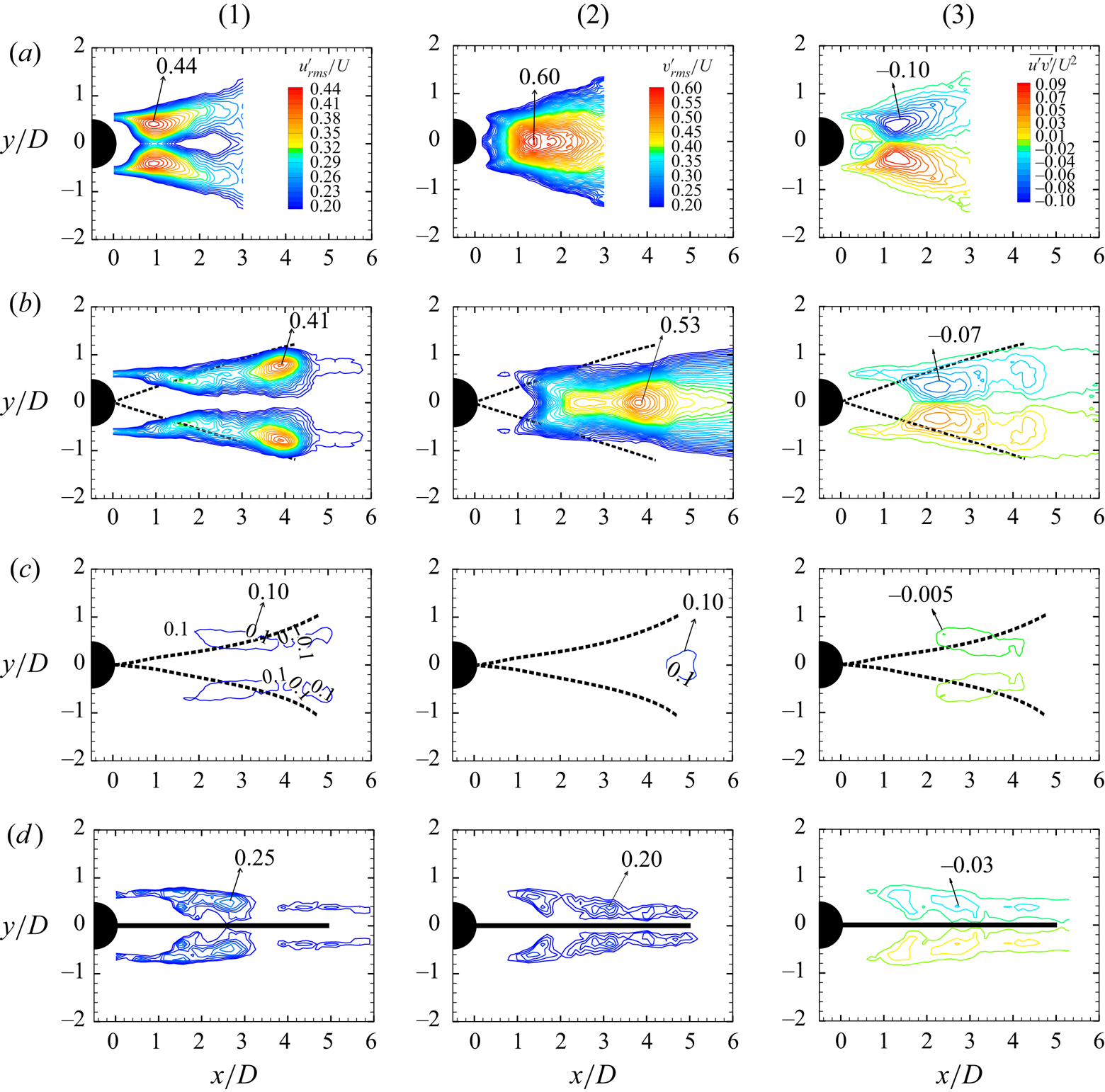
Figure 14. Contours of (1) streamwise velocity fluctuations ( $u'_{rms}/U$), (2) transverse fluctuations ( ${v'_{rms}}/U$) and (3) Reynolds shear stress ( $\overline {u' v'}/U^{2}$). The plots correspond to (a) bare cylinder, (b) mode II oscillations, (c) mode I oscillations and (d) fixed–rigid plate. The Reynolds number in all cases is 8910, and the corresponding values of $K^{*}$ are (a) 0.0, (b) $4.8\times 10^{-5}$, (c) $1.1\times 10^{-3}$ and (d) $\infty$. In each case, the streamwise velocity fluctuations ( $u'_{rms}/U$) are on the left, the transverse fluctuations ( ${v'_{rms}}/U$) are in the middle and the Reynolds shear stress ( $\overline {u' v'}/U^{2}$) are on the right. The plots show a striking reduction in streamwise, transverse velocity fluctuations and Reynolds shear stresses corresponding to the mode I oscillations.
Table 3. Comparison of the peak magnitudes of the Reynolds shear stress for the bare cylinder.
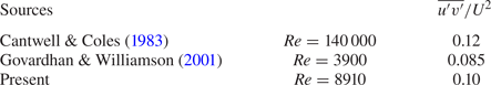
It is clear from figure 14 that there is a drastic reduction in all three components of velocity fluctuations, the streamwise, the transverse and the Reynolds shear stress, corresponding to mode I oscillations in panel (c). For example, the peak values of ( $u'_{rms}/U$) are about 0.44 for the bare cylinder in figure 14(a), 0.41 corresponding to the mode II oscillations in panel (b), whereas it is drastically lower at about 0.10 corresponding to the mode I oscillations in panel (c). It may in fact be seen that the peak values in panel (c) are lower than even the rigid splitter plate case shown in panel (d), which is about 0.25. There is clearly a large reduction in the peak values of ( $u'_{rms}/U$), and in the overall levels of ( $u'_{rms}/U$) corresponding to mode I oscillations. This is seen to be true for the transverse fluctuations ( $v'_{rms}/U$) and the Reynolds shear stress ( $\overline {u'v'}/U^{2}$) as well, as seen from the peak values for these quantities summarised in table 4 for all the four cases. There is a significant reduction in all these quantities corresponding to the mode I oscillations (in panel c) with reductions of about 80 % or more compared with the bare cylinder case (in panel a). All the three Reynolds stresses are lower than that of even the rigid splitter plate case shown in panel (d).
Table 4. Comparison of the formation length and peak values of turbulent stresses in the wake of a cylinder with a flexible splitter plate/flap. Reference cases of both a bare cylinder and a rigid splitter plate are also included. The formation length from the closure point ( $l_{form}/D$) and peak values of the three turbulent stresses ( $(u'_{rms}/U)_{max}$, $(v'_{rms}/U)_{max}$) and $(\overline {u'v'}/U^{2})_{max}$) for all the four cases are shown at $Re = 8910$.
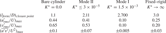
Apart from the reduction in values of the turbulent stresses, it is clear from the plots that the location of the peak values moves away from the cylinder for the flexible flap cases compared with that of the bare cylinder. This is consistent with the fact that the formation length increases in the flap cases, as the peak location of the stresses is another possible way of defining the formation length (Bearman Reference Bearman1965; Ramberg & Griffin Reference Ramberg and Griffin1974; Williamson Reference Williamson1988).
We can relate the reduction in turbulent stresses corresponding to mode I to our earlier observations of decreased lift fluctuations shown in figure 9(a). This may also be directly related to the absence of strong vortex formation at the flap tip for the mode I case, whereas there is clear vortex formation in the case of mode II flap oscillations. The formation of weaker vortices with correspondingly larger formation length in mode I may also be related to the reduced mean drag seen in mode I. These changes may likely be related to the fact that the flap oscillations in mode I are significantly smaller close to the base, whereas the oscillations in mode II are larger near the cylinder base, as may be seen in figures 3(a) and 3(b).
4. Flexible splitter plate with $L/D=2$

In this section, we present results for a flexible splitter plate/flap with a flap length to cylinder diameter ratio  $L/D$ of two. A key difference in this shorter flap case is the fact that its length is comparable to or smaller than the formation length of the wake vortices in the bare cylinder case, in contrast to the $L/D = 5$ flap case, where the flap length is considerably larger than the formation length. In this shorter flap case, even a rigid flap would not be sufficient to suppress shedding.
The  $L/D = 2$ flexible splitter plates show a greater variety of flap mode shapes compared with the $L/D = 5$ splitter plates, with these modes being dependent on $K^{\ast }$. We present in figure 15 a set of observed mode shapes in this case, which we refer to as modes A through D, respectively, with the non-dimensional flexural rigidity, $K^{\ast }$, increasing as we go from mode A to D. As shown in the figure, very flexible splitter plates (low $K^{\ast }$) exhibit large-amplitude symmetric flap motions (mode A), whereas clearly asymmetric flap motions are seen at higher $K^{\ast }$ values corresponding to modes B and C. Mode B corresponds to asymmetric large-amplitude flapping motions, whereas mode C is also asymmetric with the flap deflected off to one side, but having small oscillation amplitudes. At even higher $K^{\ast }$ values, corresponding to mode D, symmetric flap motions are again seen with the amplitudes being smaller than in mode A. It should be noted that all these modes are stable, although in some cases, as in modes C and D, they can both be seen at the same $K^{\ast }$ values, as discussed later.
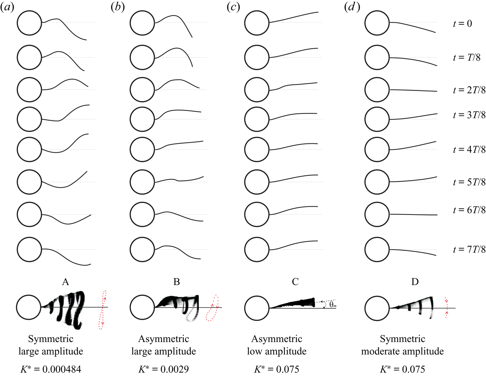
Figure 15. Time sequence of pictures showing the deformation shapes of  $L/D = 2$ flap over one oscillation cycle for the flapping modes A, B, C and D: (a) mode A flapping, $Re = 18\,131$, $K^{\ast } = 4.84\times 10^{-4}$; (b) mode B flapping, $Re = 12\,057$, $K^{\ast } = 2.9\times 10^{-3}$; (c) mode C flapping, $Re = 7577$, $K^{\ast } = 7.50\times 10^{-2}$; (d) mode D flapping, $Re = 7577$, $K^{\ast } = 7.50\times 10^{-2}$. Each of the deformation shapes is separated by one-eighth of the oscillation period, $T$. For each of the modes, the superimposed images and tip trajectories shown by a red dashed line is shown in the last row. Supplementary movies 3, 4, 5 and 6 show the temporal behaviour of flap deformations corresponding to modes A, B, C and D, respectively.
We present results for a flexible  $L/D = 2.0$ flap in the wake of a circular cylinder in three subsections. In the first subsection, we discuss the flap kinematics, where we present the response of the flaps and how it is modified by variations in flexural rigidity $EI$. This is followed in the second section by force measurements where we present the results of the fluctuating lift forces and the mean drag of the cylinder–splitter plate combination. In the third section, we present results from PIV measurements of the wake vortex dynamics.
4.1. Flap kinematics
The deformation of the  $L/D = 5$ flexible splitter plates/flaps is in the form of a travelling wave, as discussed in § 3. This is true for both the periodic mode I and mode II oscillations. In the present case of a $L/D = 2$ flexible splitter plate/flap, the mode A and B oscillations at low $K^{\ast }$ values are again in the form of a travelling wave as can clearly be seen from the deformed shapes of the $L/D = 2$ flap shown in figure 15, over a cycle of the flap tip motion. At higher $K^{\ast }$ values corresponding to mode C, the deflected small-amplitude oscillations correspond to the first bending mode of the plate/flap. In mode D, the deformations of the plate again correspond to the first bending mode, but are symmetric.
We present in figure 16 the response of the  $L/D = 2$ configuration as a function of the normalised flexural rigidity values ( $K^{\ast }$). This response data are taken from four different flexural rigidity ( $EI$) value flaps, which together enables us to cover a wide range of $K^{\ast }$ values to see all the modes (A to D). The figure shows both the non-dimensional flap tip amplitude (in figure 16a) and the frequency response (in figure 16b) with $K^{\ast }$. At the lowest $K^{\ast }$ values, we have large-amplitude symmetric motions corresponding to mode A. As $K^{\ast }$ is increased from these low values, we obtain asymmetric large- and small-amplitude motions corresponding to mode B and C, respectively. As seen from the plot, mode C coexists with mode D over a range of $K^{\ast }$ values demarcated by the grey shaded region, with the latter corresponding to symmetric larger-amplitude flap motions. Within this range of $K^{\ast }$ values, the flap is seen to choose one of the two modes depending on the initial conditions, and could be triggered to choose the other mode by providing an external perturbation to the flap. At even higher $K^{\ast }$ values, only mode D is seen, and its amplitude rapidly decreases to small values as $K^{\ast }$ is further increased. The non-dimensional frequencies of oscillation corresponding to the different modes can be seen in figure 16(b), with modes A and B having values around 0.2. In contrast, the small amplitude deflected oscillations corresponding to mode C have much lower frequencies, while the symmetric oscillations of the higher $K^{\ast }$ mode D oscillations are distinct from both that of mode B and C with values of approximately 0.15 at the lowest $K^{\ast }$ values of mode D and slowly increasing with $K^{\ast }$ to about 0.2 as the amplitude drops to very small values.
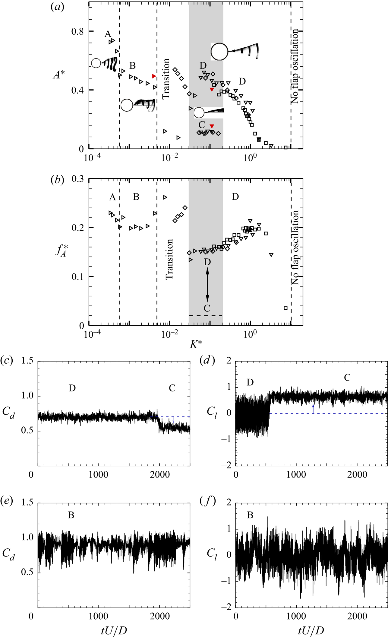
Figure 16. (a) Amplitude,  $A^{\ast }$ and (b) frequency, $f^{\ast }_{A}$ response of the tip oscillation with non-dimensional bending stiffness, $K^{\ast }$ for different flexural rigidity, $EI$:
$EI$:  $\triangleright$, $EI = 2.70\times 10^{-5}$ N m; $\diamondsuit$, $EI = 7.50\times 10^{-4}$ N m; $\nabla$, $EI = 2.75\times 10^{-3}$ N m; $\square$, $EI = 1.25\times 10^{-2}$ N m. In (a), all data shown by open symbols correspond to the large tunnel, whereas the solid red symbols represent data from the smaller tunnel used for PIV measurements. Sample time traces of the fluctuating drag and lift force signals corresponding to flapping modes B, C and D are also shown for two different values of $K^{\ast }$. Panels (c) and (d) show $C_{l}$ and $C_{d}$ signals, respectively, for spontaneous transition between flapping modes D and C that occur in the shaded regime of the response at $Re = 7577$, $K^{\ast } = 7.50\times 10^{-2}$. Panels (e) and (f) show $C_{l}$ and $C_{d}$ signals, respectively, for flapping mode B at $Re = 13\,618$, $K^{\ast } = 2.3\times 10^{-2}$.
In order to encourage the flapping mode C over a range of flow speeds a couple of different types of flap configurations were studied with a flap of flexural rigidity,  $EI = 7.50\times 10^{-4}$ N m. In one flap type, many small holes were provided in a staggered pattern over the rear half portion of the flap, which we refer to as type I. In the other type of flap, the entire flap was split into a number of smaller flaps having spanwise length of $1 D$, which we refer to as type II. Schematics of these two flap types are given in figure 17. The oscillation amplitude and frequency of the flap tip for these two different flap configurations are shown in figure 18(a) and figure 18(b), respectively, along with the data for the normal configuration discussed earlier (indicated by $\diamondsuit$). It is clear from the data that the type I configuration (shown by $\circ$) encourages the existence of the deflected mode C in comparison to the larger oscillation amplitude mode D. Over the range of $K^{\ast }$ values corresponding to the shaded area and a little beyond, we see that the type I flap always shows mode C behaviour with no evidence of mode D. It appears that the larger damping associated with the fluid being pushed through the holes of the flap encourages mode C and discourages mode D. This may be a good practical way of increasing (‘structural’) damping with the present type of flexible flaps.
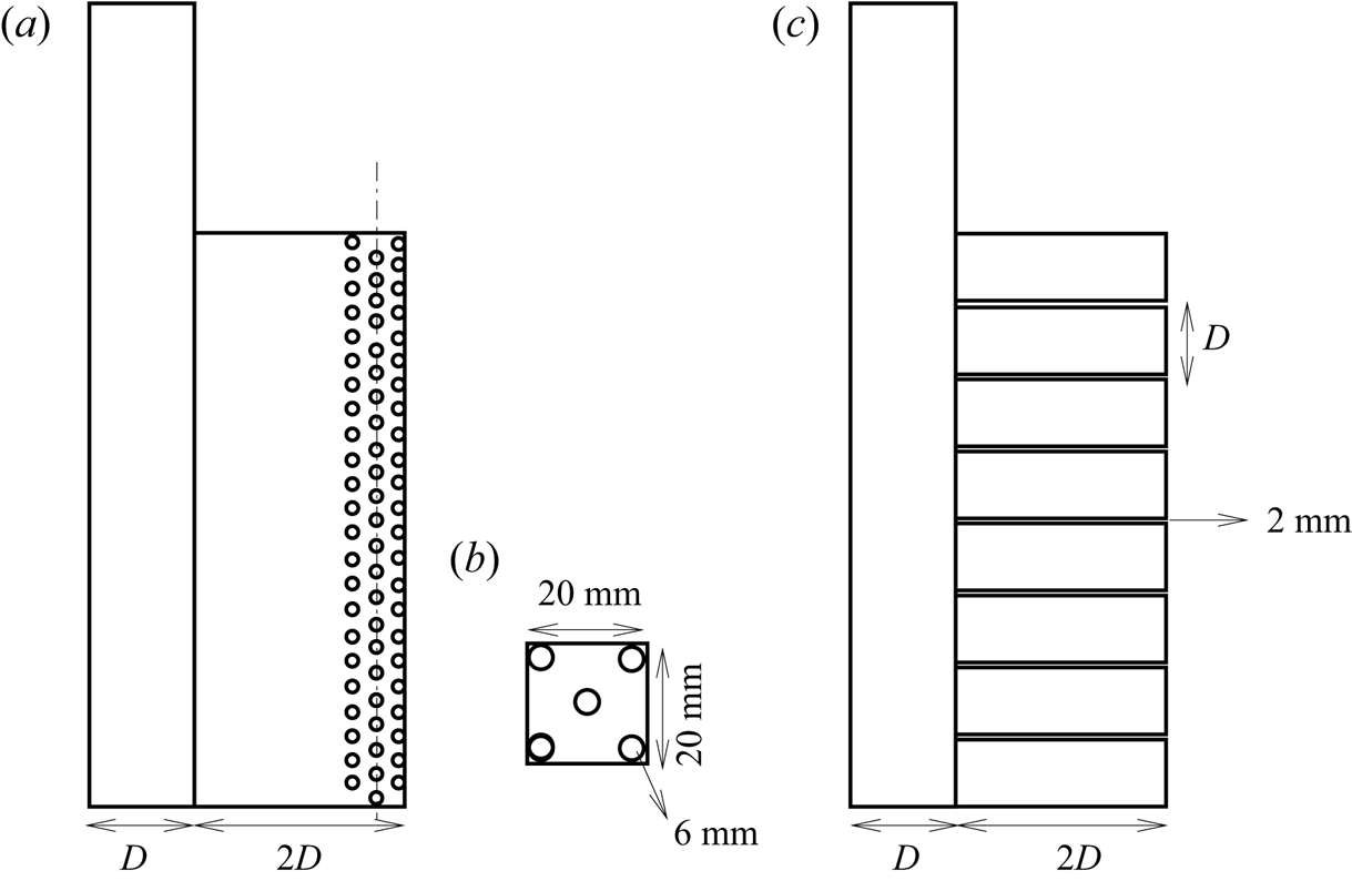
Figure 17. Schematic showing the different types of short flexible splitter plate/flap. (a) Staggered holes pattern whose unit cell is shown in (b). (c) Pattern of the split flaps.
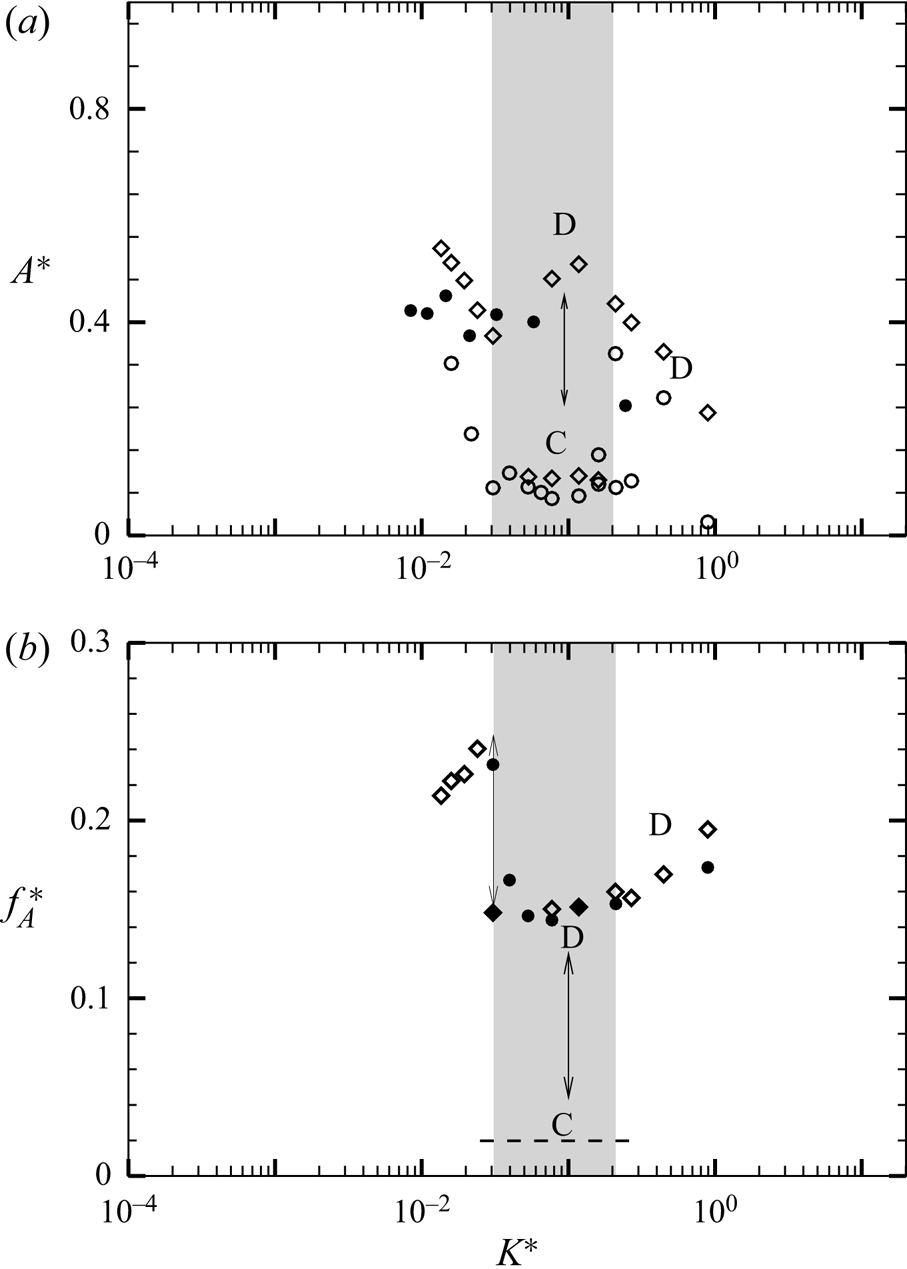
Figure 18. Plots of (a) oscillation amplitude ( $A^{\ast }$) and (b) frequency response ( $\,f^{\ast }_A$) for the two different configurations of short flexible splitter plate referred to as type I and type II flaps. The type I flap (shown by $\circ$) comprises a set of staggered holes on the rear half of the flap, whereas the type II flap (shown by $\bullet$) consists of a set of split flaps with spanwise size of $1D$. The normal flexible flap, without holes and in one single piece (without splitting) case is also shown in the plot ( $\diamondsuit$). Here $L/D=2.0$ and $EI = 7.50\times 10^{-4}$ N m.
In contrast to the type I flaps, we find little difference between the type II flaps and the normal flexible flaps. The type II amplitude data, also shown in figure 18(a) ( $\bullet$), lies almost close to the normal flap case (shown in $\diamondsuit$). It should be noted that the flapping amplitude and frequency of the split flap (type II) was measured at the central split flap, and in general this may not represent the response of the other split flaps. There is also the possibility of a phase difference among motions of adjacent split flaps that can lead to reduced spanwise correlation of the wake vortices, which can, in turn, cause a reduction in the fluctuating forces. Split flaps like the type II case of flap have been shown to suppress VIVs of a circular cylinder by Kim & Lee (Reference Kim and Lee2012). In our case, the split flaps have a spanwise length of $1D$ and a streamwise length of $2D$.
$2D$.
The least  $EI$ flap showed some $Re$ effect at low speeds. This can be seen from its response shown by right triangle in figure 16 at $K^{\ast } \approx 0.01$, where two points are much lower than the other data at higher speeds or lower $K^{\ast }$. These points correspond to lower $Re$ ( $Re < 5000$), and may be affected by $Re$ as seen in the fluctuating lift forces on a bare cylinder case earlier. This is similar to the response of the $L/D = 5$ , which are affected by $Re$ for $Re < 5000$. It is important to note that this effect was seen only for this flap, and higher $EI$ flaps for this shorter flap case did not show any $Re$ effects.
In summary, figure 16 shows all the different modes that occur for the  $L/D = 2$ flap case, with the modes being dependent on $K^{\ast }$. At low values of $K^{\ast }$, symmetric large-amplitude mode A is seen, which is followed by asymmetric modes B and C as $K^{\ast }$ is increased, with the latter corresponding to a deflected flap with small-amplitude oscillations. In the shaded region, both modes C and D exist at the same flow speed, with the symmetric smaller amplitude mode D continuing to be seen at even higher $K^{\ast }$ values.
The modes discussed previously have striking similarities with the recent numerical study of flexible splitter plates for  $L/D = 2.0$ done at low Reynolds numbers ( $Re = 80$) by Pfister & Marquet (Reference Pfister and Marquet2020). In their work at low $Re$, they present five modes, referred to as R1 to R5, with R1 corresponding to high flexural rigidity and R5 the lowest flexural rigidity. Although the flow regimes are significantly different in the present experimental work, there are broad similarities with the presence of both symmetric and asymmetric flapping modes in both cases. In particular, we can see that the symmetric large and small-amplitude mode A and mode D in the present work are similar to their R4 and R2 modes, respectively, whereas the deflected small-amplitude mode C is similar to their R3 mode. The flexural rigidity values of Pfister & Marquet (Reference Pfister and Marquet2020) have been converted to the presently used $K^{\ast }$ parameter and the ranges of their different modes along with the range of $K^{\ast }$ values for the present modes is listed in table 5. it may be seen that the range of $K^{\ast }$ parameter corresponding to similar modes in the two cases have significant differences, which may be related to the different flow regimes. Apart from this numerical differences, it should be noted that there are qualitative differences as well, such as the presence of the large-amplitude asymmetric mode B in the present case, which is not seen at low $Re$.
$Re$.
Table 5. Ranges of the non-dimensional bending stiffness or  $K^{\ast }$ corresponding to different flapping modes in the present work and in those of Pfister & Marquet (Reference Pfister and Marquet2020). The left column presents the modes corresponding to present data and the right column represents the flapping modes defined by Pfister & Marquet (Reference Pfister and Marquet2020) for $L/D = 2$ at $Re = 80$. R1, no flap oscillation; R2, symmetric and periodic; R3, deviated and periodic; R4, symmetric and periodic; R5, symmetric and quasi-periodic.
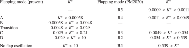
4.2. Force measurements
The flap exhibits different flapping modes depending on the value of  $K^{\ast }$ as discussed previously. Most of these modes of flapping (A, B and D) exhibit a strong periodic oscillation with large amplitude of the order of about $0.5D$, whereas flapping mode C demonstrated a deflected state of the flap with very small flap motions. This mode C of the cylinder–flap configuration appears to be nearly steady at a deflected state with a mean angle to the flow direction. This type of deflected flap (for a hinged case) has been shown by Assi et al. (Reference Assi, Bearman and Kitney2009) to be effective in suppression of VIV. In this section, we report on the variation of the measured drag and fluctuating lift force as a function of $K^{\ast }$.
We first present some time traces of the measured drag and lift forces acting on the cylinder. In particular, we choose two example  $K^{\ast }$ values, one corresponding to the shaded grey region in figure 16, where both modes C and D coexist, and the other corresponding to the asymmetric mode B. The drag and lift times traces corresponding to the grey shaded region are shown in figures 16(c) and 16(d), respectively. The first point to be noted is that the two measurements are not simultaneous and, hence, both need to be seen as independent measurements. In both time traces, there is a clear sudden and spontaneous change of the forces at some point in time, which is the transition from mode D to mode C. As the flapping switches to the deflected small-amplitude mode C, the mean of the drag force reduces to lower values than in the symmetric mode D, and we give reasons for this from the PIV measurements in the following section. Similar spontaneous change from mode D to C can also be seen in the sample lift time trace taken at the same $K^{\ast }$ (shown in figure 16d). In this case, one can see the sudden development of a mean lift as the flap assumes a deflected position in mode D. One can also see a large decrease in the fluctuating lift in this mode C state, which is related to large reduction in flapping amplitude seen earlier in figure 16(a) and consequently show the suppression in vortex formation discussed in the subsequent section.
Drag and lift time traces corresponding to the asymmetric mode B flapping are shown in figures 16(e) and 16(f), respectively. It is clear from time traces of the fluctuating drag force coefficient in figure 16(e) that the fluctuating drag forces are amplified due to the asymmetric mode of flapping, which also slightly increases the mean value of drag force. The fluctuating lift coefficient (in figure 16f) is seen to exhibit a strong asymmetry, as seen from the local mean value, which is seen to vary with time.
We shall now present the measured fluctuating lift and mean drag force as a function of  $K^{\ast }$, using as before flaps of different flexural rigidities ( $EI$) to obtain a wide range of $K^{\ast }$. The fluctuating lift and mean drag have been normalised by the respective values for the bare cylinder at the same $Re$, and the resulting normalised fluctuating lift ( $C_{l'}^{\ast }$) and mean drag ( $\overline {C^{\ast }_{d}}$) are shown in figures 19(a) and 19(b), respectively.
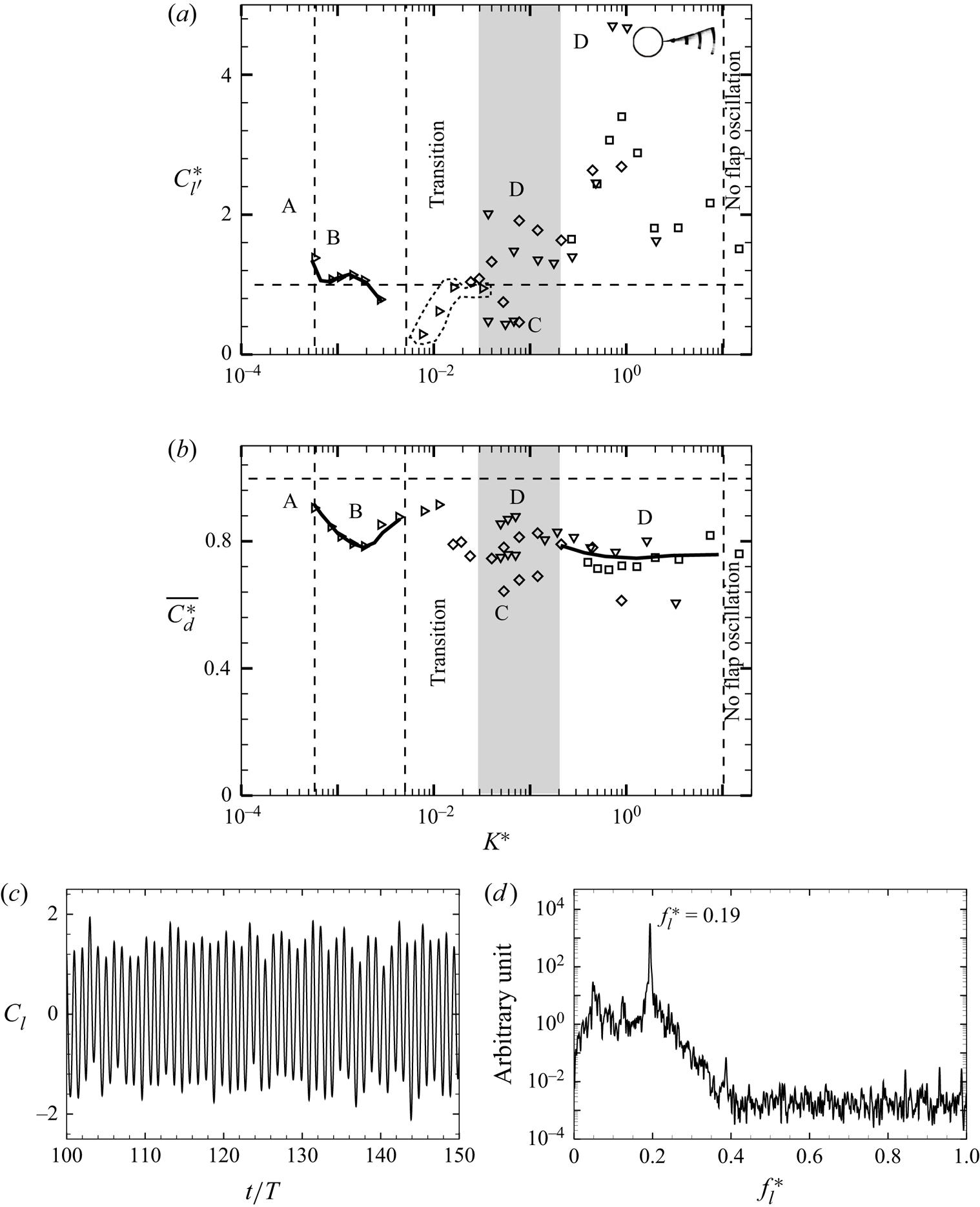
Figure 19. Plots of normalised (a) r.m.s. lift force,  $C_{l'}^{\ast }$ and (b) mean drag force coefficient, $\overline {C^{\ast }_{d}}$ with $K^{\ast }$ for flaps with different $EI$:
$EI$:  $\triangleright$, $EI = 2.70\times 10^{-5}$ N m; $\diamondsuit$, $EI = 7.50\times 10^{-4}$ N m; $\nabla$, $EI = 2.75\times 10^{-3}$ N m; $\square$, $EI = 1.25\times 10^{-2}$ N m. Maximum reduction in $C_{l'}^{\ast }$ is found at mode B and mode C in the deflected state of flapping shown in shaded regime $[E \leftrightarrow D]$ of the plots. The peak in $C_{l'}^{\ast }$ is linked to the resonant condition and the corresponding time trace and spectrum of the fluctuating force signals are shown in (c) and (d), respectively. The $\overline {C_{d}^{\ast }}$ shown in (b) gradually decreases as the $K^{\ast }$ increases except for the shaded regime in the plot, where mean drag force further abruptly drops to lower values when the flap attains mode C.
The normalised fluctuating lift ( $C_{l'}^{\ast }$) in figure 19(a) shows distinctly different trends depending on the flapping mode. At low values of $K^{\ast }$, corresponding to mode A and B, the fluctuating lift is close to that of the bare cylinder values, and hence $C_{l'}^{\ast }$ is close to unity. As $K^{\ast }$ is further increased, we reach the shaded region within which both mode C and D coexist. Here, the lower values of $C_{l'}^{\ast }$ correspond to the deflected mode C, as was seen earlier with the time traces. The deflected flap has both lower oscillations and suppresses the shedding, both contributing to the reduction in fluctuating lift. Mode D on the other hand has higher values of $C_{l'}^{\ast }$ compared with that of the bare cylinder within this shaded regime. As we further increase $K^{\ast }$, the $C_{l'}^{\ast }$ values dramatically increase reaching a peak at $K^{\ast } \approx 0.8$, after which the values reduce. This peak in $C_{l'}^{\ast }$ found in mode D occurs as discussed earlier for the $L/D=5$ case when the wake frequency is close to the structural first bending mode frequency of the flap; both of which are close to about 0.20 in this $L/D$ case. It may be noted that the structural first bending mode frequency required as estimate of the fluid added mass, and was computed here in the same manner as described earlier for the $L/D=5$ case. The corresponding amplitude and frequency of the flap tip close to this peak in $C_{l'}^{\ast }$ is shown in figure 20(b), and as before shows a relatively flat amplitude response and a local peak in frequency. As discussed earlier, the reason for the peak in $C_{l'}^{\ast }$, which is much larger in this $L/D=2$ case, needs further study.
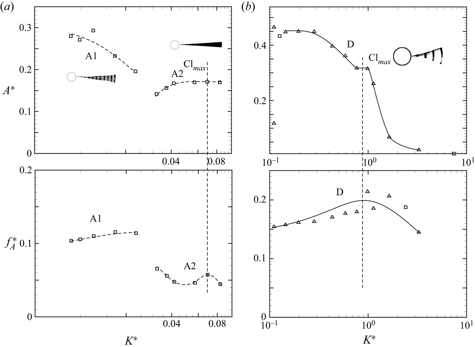
Figure 20. Amplitude and frequency response of the flap tip close to the maximum  $C_{l'}^{\ast }$ for (a) $L/D=5$ and (b) $L/D=2$: $\nabla$, $EI = 2.75\times 10^{-3}$ N m; $\square$, $EI = 1.25\times 10^{-2}$ N m.
The normalised mean drag ( $\overline {C_{d}^{\ast }}$) in figure 19(b) also shows differences depending on the flapping mode. The lowest drag is found to occur in mode C and parts of mode D with 30–40 % drag reduction compared with the bare cylinder case. It may however be noted that the drag is in general lower than the bare cylinder case at most $K^{\ast }$ values. The largest value of drag occurs at very low $K^{\ast }$ values where the drag is close to that of the bare cylinder. The variation of drag with $K^{\ast }$, and the low drag seen in mode C regime will be discussed further in the next section in relation to the measured values of the formation length.
4.3. PIV measurements
We present here PIV measurements of the flapping modes B, C and D. Flapping mode A could not be achieved in the smaller water tunnel, where these experiments were conducted due to flow speed limitations there. We first present the phase-averaged vorticity fields to show the different modes of vortex formation. This is followed by mean and turbulence flow fields corresponding to these flapping modes along with two reference cases of the bare cylinder and the fixed–rigid splitter plate.
Figure 21 presents the phase-averaged vorticity fields during half cycle of the tip oscillations shown from panel (a) to panel (d) for the flapping modes B, C and D. It is clear from the figure that a single vortex is formed during the half cycle of flap tip oscillation shown from panel (a) to panel (d) for flapping modes B and D, indicating a 2S mode of vortex formation in the terminology of Williamson & Roshko (Reference Williamson and Roshko1988). The white region in the flapping mode D shown in the figure represents the extent of motions of the flap, whose trajectory appears to follow a curvilinear path with very small variation in streamwise direction as mentioned earlier. In case of the flapping mode C, where the flap adopted a stable position deflected to one side of the wake with small flap tip oscillations, the formation of vortices is almost inhibited and only weak vortices formed near the flap tip at particular location of flap tip. In this case, due to the small motions of the flap, there are very little differences in the vorticity plots at different locations of the flap tip. As may be seen from the figure, the shear layers on the two sides of the flap in this case move along the flap and form weak vortices near the tip.
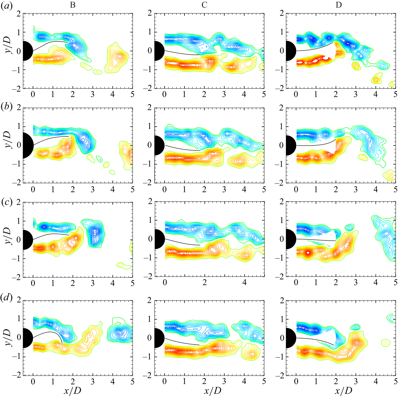
Figure 21. Phase-averaged vorticity plots reveal evolution of flow fields during half cycle of the flapping modes B, C and D for the short flap case. It shows that a single vortex is shed during each half cycle of the flap oscillation shown from (a) to (d) in case of modes B and D corresponding to a 2S mode of vortex formation, whereas in mode C shown in (c) the shear layers on the two sides of the flap move along the flap and form weak vortices near the tip. Vorticity contours levels shown are  $\omega D/U$ = $\pm$0.5, $\pm$0.75, $\pm$1.0, $\pm 1.5,\ldots, \pm 5.0$.
Mean velocity fields of the cylinder wake were obtained from the time average of a large ensemble ( $\approx$1000) of instantaneous PIV velocity vector fields. Figure 22 shows streamline plots of the mean velocity fields and corresponding mean vorticity fields for different flapping modes along with two reference cases of the bare cylinder (in figure 22a) and the fixed–rigid splitter plate [ $K^{*} \rightarrow \infty$] (in figure 22e). The flapping envelope of the flap cases is shown by solid lines, whereas in figure 22(e), the solid line represents the fixed–rigid splitter plate. The filled circle in the plots shows the location of the closure point in the centre of the wake, where the mean streamwise velocity is zero. Formation length based on the closure point is found to be higher for mode C corresponding to the deflected flap state, compared with modes B and D. The highest formation length is however found to be for the limiting case of the fixed–rigid splitter plate shown in figure 22(e). This variation of the formation length with $K^{\ast }$ is shown in figure 23, with the formation length in most cases being larger than that of the bare cylinder case. The normalised mean drag coefficient ( $\overline {C_{d}^{\ast }}$) variation found earlier is consistent with this variation of the formation length, with the drag in most cases being lower than the bare cylinder case, and the large reduction in drag corresponding to mode C being correlated to the large increase in formation length for this mode.
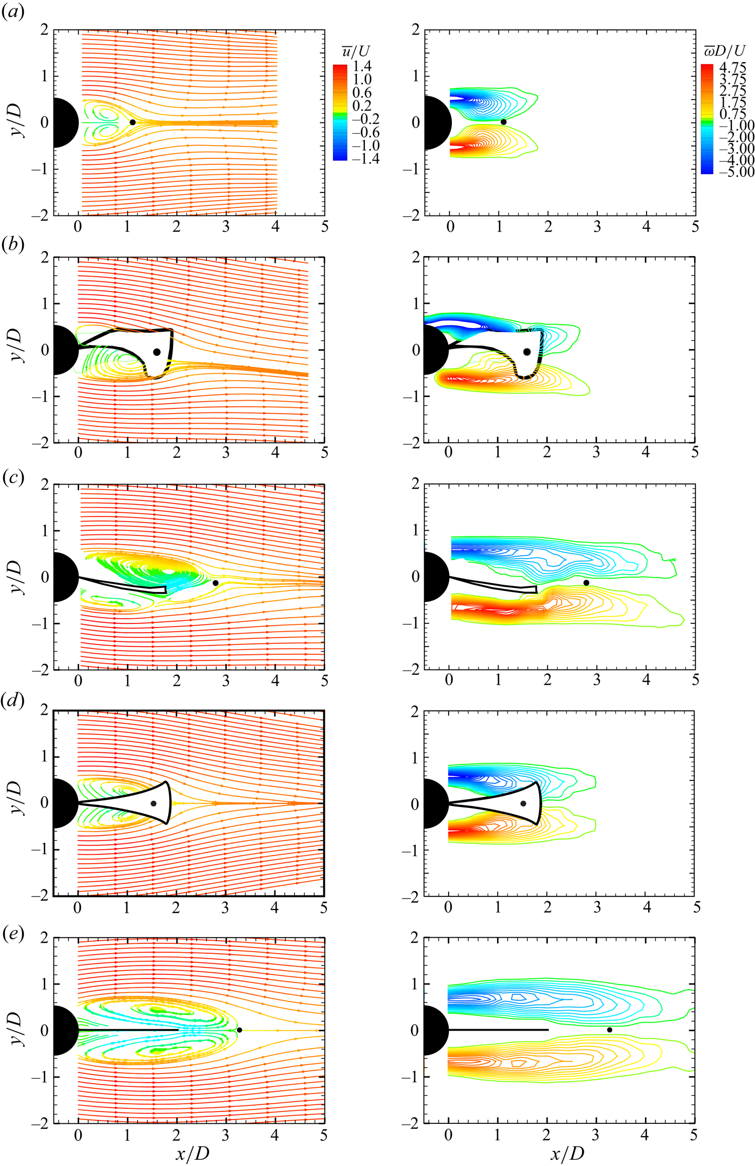
Figure 22. Mean stream line (left) and mean vorticity field (right) corresponding to (a) bare cylinder, (b) mode B, (c) mode C, (d) mode D and (e) fixed–rigid splitter plate:  $L/D = 2$ case with $Re=8910$.
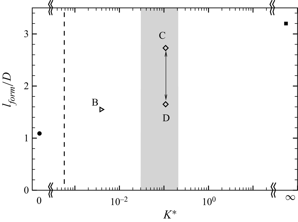
Figure 23. Variation of the formation length,  $l_{f}$, with $K^{\ast }$: $\triangleright$, $EI = 2.70\times 10^{-5}$ N m; $\diamondsuit$, $EI = 7.50\ \times $ $10^{-4}$ N m. The plot demonstrates that formation is continuously pushed away from the cylinder with increasing $K^{*}$, with a sudden increase corresponding to mode C having the deflected flap. Horizontal axis is broken to adjust the two extreme values of $K^{\ast }$ shown for the reference cases of bare cylinder ( $\bullet$) and fixed–rigid splitter plate ( $\blacksquare$).
Response of the fluctuating forces has shown an increase in the magnitude of fluctuating lift force particularly in mode D. There was also a drop in the drag force, which was associated with the increase in the formation length compared with the bare cylinder case. In order to gain more insight into variation of these quantities in different flapping modes, and to see how it affects the flow fields, we present the turbulence statistics for the different modes and the two reference cases. The turbulence quantities presented are the streamwise turbulence intensity ( $u'_{rms}/U$), transverse turbulence intensity ( $v'_{rms}/U$) and the Reynolds shear stress ( $\overline {u'v'}/U^{2}$).
Figure 24 presents contours of (1) streamwise and (2) transverse turbulence intensities and (3) Reynolds shear stress at the flapping modes B, C and D along with two reference cases of the bare cylinder and the fixed–rigid splitter plate case. It is apparent that the maximum contours level of the  $u'_{rms}/U$ ( $=$ 0.53) and $\overline {u'v'}/U^{2}$ ( $=\pm$ 0.13) occur in flapping mode D, with both these values being significantly higher than for the bare cylinder case. However, maximum values of the $v'_{rms}/U$ ( $=$ 0.53) is slightly reduced compared with that for the bare cylinder values, which is about 0.60. Locations of $(u'_{rms}/U)_{max}$, $(v'_{rms}/U)_{max}$ and $(\overline {u'v'}/U^{2})_{max}$ are found to be shifted downstream compared with the corresponding locations of these quantities of the bare cylinder case, indicating, as before, an increase in the formation length.
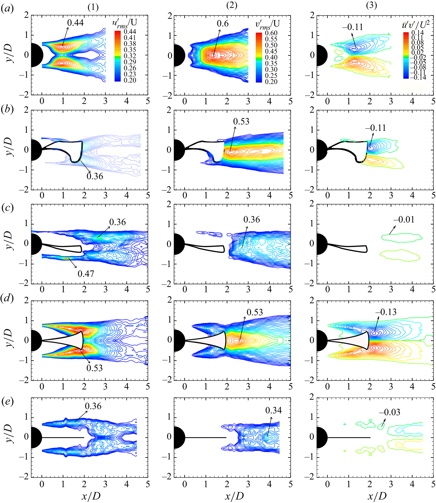
Figure 24. Contours of (1) streamwise fluctuations ( $u'_{rms}/U$), (2) cross-stream fluctuations ( $v'_{rms}/U$) and (3) Reynolds shear stress ( $\overline {u'v'}/U^{2}$) corresponding to (a) bare cylinder, (b) mode B, (c) mode C, (d) mode D and (e) fixed–rigid splitter plate. The maximum reduction in $u'_{rms}/U$, $v'_{rms}/U$ and $\overline {u'v'}/U^{2}$ is found in mode C and the limiting case of the fixed–rigid splitter plate [ $K^{\ast } \rightarrow \infty$]. Mode D shows the maximum increase (16.9 %) of $u'_{rms}/U$ and (30 %) $\overline {u'v'}/U^{2}$, whereas $v'_{rms}/U$ is slightly reduced (11.6 %) from that for the bare cylinder.
The fall in the  $\overline {C_{d}^{\ast }}$ and the non-dimensional flapping frequency, $f_{A}^{\ast }$ is consistent with PIV measurements of the turbulence related quantities and also with the mean flow fields. The PIV measurements of turbulence and the mean flow fields suggest an increase in the formation length, which is consistent with the reduction of $f_{A}^{\ast }$ and $\overline {C_{d}^{\ast }}$ seen earlier. The growth in the transverse fluctuating forces in the flapping mode D can also be explained by contours of the streamwise turbulence intensity showing a larger level of contours values close to the cylinder base in comparison with corresponding contours levels of the bare cylinder case. This increment in the strength of fluctuations also increased $\overline {u'v'}/U^{2}$ as may be seen from the contours in figure 24(3) compared with the corresponding case of the bare cylinder shown in figure 24(a). The most interesting configuration of flapping mode C, where the oscillation of the tip is almost inhibited, shows a large reduction of the turbulence intensities. This reduction is about 19 % in streamwise and cross-stream turbulence intensities and about 90 % in the Reynolds shear stress. This change in the turbulence statistics can also be seen in figure 25. Figure 25 shows cross-stream variation of turbulence intensities and Reynolds shear stress at $x/D = 2.0$ just downstream of the flap. This plot shows again the large reductions, especially in Reynolds shear stress in flapping mode C, which is very close to the reference case of the fixed–rigid splitter plate, or even lower in the case of the Reynolds shear stress. The peaks magnitude of these turbulence quantities are also listed in table 6. This drastic change in the wake characteristics particularly in flapping mode C suggests the formation of very weak vortices, which could be useful to suppress VIV compared with the other flapping modes.
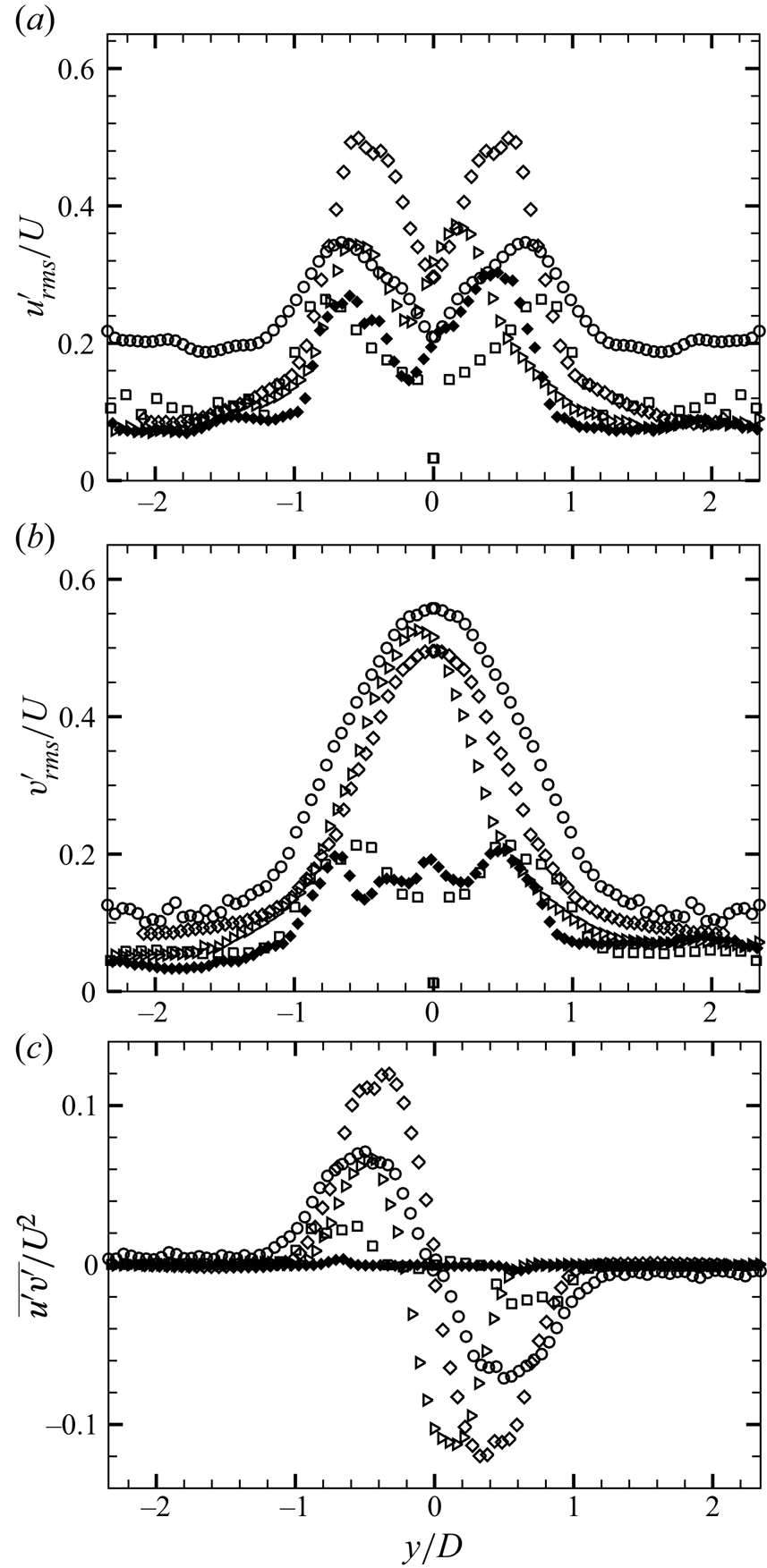
Figure 25. Transverse variation of turbulence statistics at  $x/D = 2.0$ for the different flapping modes along with reference cases of the bare cylinder and limiting case of the fixed rigid splitter plate: $\circ$, bare cylinder; $\triangleright$, mode B; $\diamondsuit$, mode D; $\blacklozenge$, mode C; $\square$, fixed–rigid splitter plate. Mode C shows a maximum reduction in turbulence related quantities, with in particular the Reynolds shear stress being substantially reduced ( $\approx$90 %).
Table 6. Peak magnitudes of turbulence statistics of the cylinder–flap system for the different flapping modes of the flap motion along with corresponding values of the reference case of the bare cylinder and the fixed–rigid splitter plate.
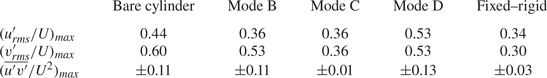
5. Concluding remarks
We have systematically varied the flexural rigidity ( $EI$) of the $L/D = 5$ and $L/D = 2$ flexible splitter plates/flaps over a large range of values, and found that the results for flap tip motion and forces collapse well when plotted with a non-dimensional bending stiffness ( $K^{\ast }$), which is defined as $K^{\ast }=EI/((1/2)\rho U^2 L^3)$. This collapse occurs across flexible flaps with different values of $EI$, as long as $Re>5000$. We have found that the collapse is not good for $Re<5000$. This difference appears to be related to the reduction in fluctuating lift for a bare cylinder in the $Re$ range between about 1600 and 5000 discussed by Norberg (Reference Norberg2003). We have found that the flap motions (for $Re > 5000$), forces and wake fields show distinct differences as $K^{\ast }$ is varied, and these differences in response with $K^{\ast }$ are clearly summarised in figure 26 for both the $L/D=5$ and $L/D=2$ flexible flaps.
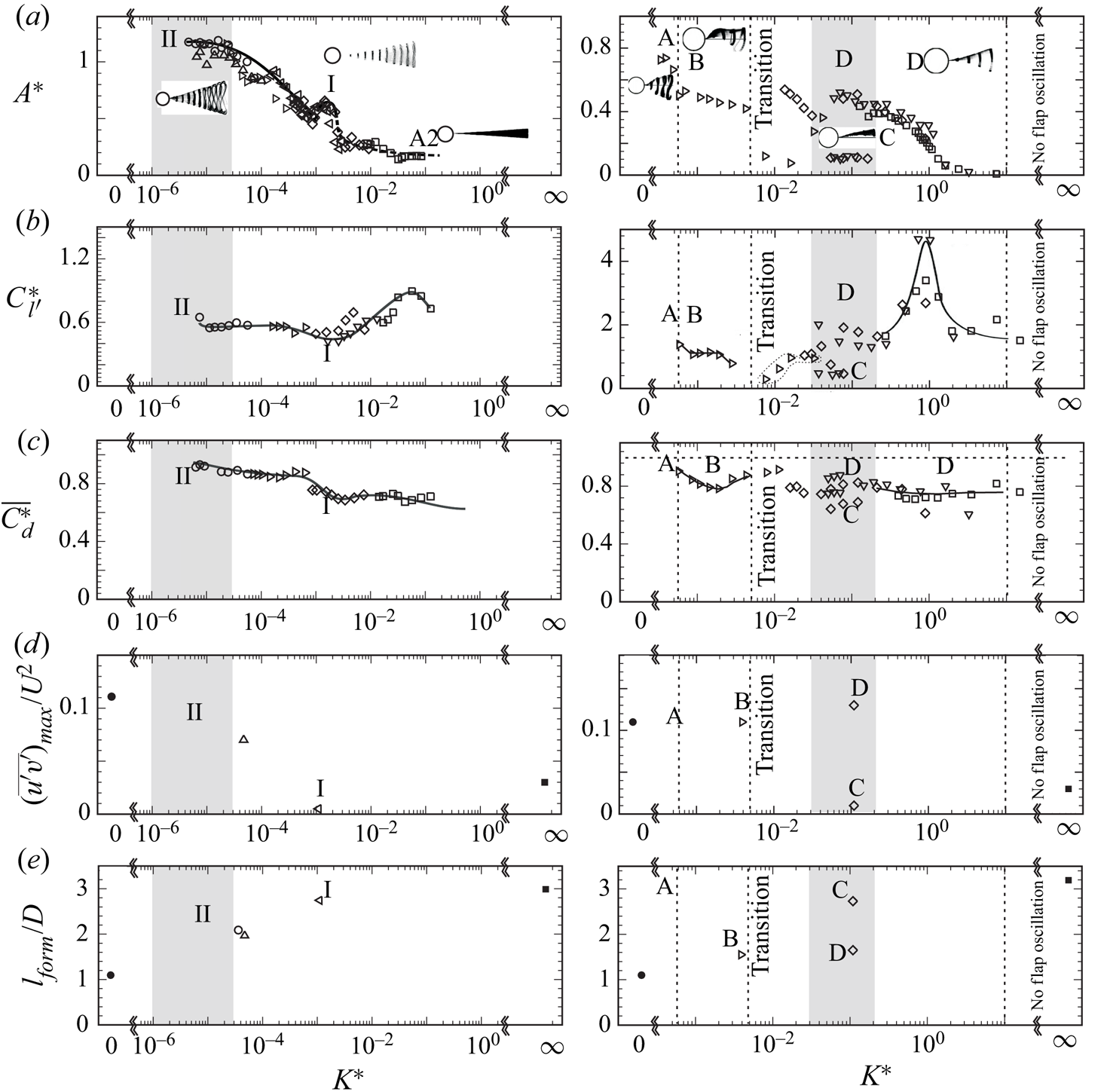
Figure 26. Plots of  $A^{\ast }$, $C_{l'}^{\ast }$, $\overline {C_{d}^{\ast }}$, $\overline {(u'v')}_{max}/U^{2}$ and $l_{form}/D$ with the non-dimensional bending stiffness, $K^{\ast }$ for (a) $L/D = 5$ and (b) $L/D = 2$ flaps.
Response of  $L/D = 5$ flaps exhibit two periodic regimes of flap deformations in the form of travelling waves within the range of $K^{\ast }$ values from $5\times 10^{-6}$ to $1\times 10^{-1}$ studied. The first corresponds to a local peak in flap tip amplitude at $K^{\ast } \approx 1.5\times 10^{-3}$ that we refer to as mode I, and the second that occurs at low values of $K^{\ast }$ ( $K^{\ast }<3\times 10^{-5}$) that we refer to as mode II. Apart from differences in the flap tip amplitude between these two periodic modes, there are also differences in the magnitude of the streamwise oscillations and its phase with respect to the cross-stream oscillations, the latter resulting in differences in the figure-of-eight shape traversed by the flap tip in the two cases. The non-dimensional frequency of flap tip motions ( $\,f^{\ast }_A=fD/U$) also shows changes between the two flapping modes. These differences lead to large changes in the vortex formation between the two cases, with only weak vortices being formed in the mode I case unlike the mode II case, where clear strong vortex formation can be seen at the flap tip as in the case of the bare cylinder. The weak formation of vortices in mode I leads to the lowest values of fluctuating lift for this mode, whereas the mean drag is found to reach a broad minimum that starts at $K^{\ast }$ corresponding to mode I oscillations and continues for all higher $K^{\ast }$ values, with the associated drag representing an approximately 35 % reduction compared with the bare cylinder drag. At high $K^{\ast }\approx 1\times 10^{-2}$, the non-periodic and asymmetric mode A1 can be seen, whereas the other non-periodic mode A2, is seen at even higher $K^{\ast } \approx 5\times 10^{-2}$, the latter having deformations in the form of the first bending mode. A clear peak in fluctuating lift is also present within mode A2 and corresponds to the wake frequency being close to flap's structural first bending mode frequency. The corresponding wake measurements for the $L/D = 5$ flap case also show significant changes with $K^{\ast }$ in line with the observations made here. The formation length ( $l_{form}/D$) found from the closure point of the mean separation bubble is found to continuously increase with $K^{\ast }$, reaching values of about 2.6 at mode I and thereafter only small increases are seen as we go to the rigid splitter plate case corresponding to infinite values of $K^{\ast }$. This is consistent with observations of the mean drag discussed previously. The streamwise and cross-stream turbulent intensities and the Reynolds shear stresses are all found to be strikingly lower in the mode I case compared with the bare cylinder case. Importantly, these values are even lower than the rigid splitter plate case, indicating that the motions of the flap relative to the formed vortices, are such as to minimise the velocity fluctuations and the strength of the shed vortices. This is consistent with the minimum in fluctuating lift found in the mode I case.
In the  $L/D = 2$ flap case, we find that there exists a richer set of flapping modes compared with the $L/D = 5$ flap, with these modes being dependent on $K^{\ast }$. At low $K^{\ast }$ values, the flap exhibits large-amplitude symmetric flap motions that we refer to as mode A, whereas clearly asymmetric flap motions are seen at higher $K^{\ast }$ values corresponding to modes B and C. Mode B corresponds to asymmetric large-amplitude flapping motions, whereas mode C is also asymmetric with the flap clearly deflected off to one side, but having small oscillation amplitudes. At even higher $K^{\ast }$ values, corresponding to mode D, symmetric flap motions are again seen with the amplitudes being smaller than in mode A. Apart from the flap tip amplitude, the non-dimensional frequency of flap tip motions ( $\,f^{\ast }_A=fD/U$) also changes with the flap oscillation modes. In this $L/D = 2$ case, the lowest fluctuating lift and mean drag are found to correspond to mode C oscillations, with an approximately 35 % drag reduction compared with the bare cylinder drag. The PIV measurements in the wake show that is related to the weak vortices being formed in mode C case. As in the case of the $L/D = 5$ flap, there is a peak in fluctuating lift at higher values of $K^{\ast }$ corresponding to mode D where the wake frequency is close to the flap's structural first bending mode frequency. In this case, the increase in fluctuating lift is considerably larger than in the $L/D=5$ case. The wake measurements for the $L/D = 2$ flap, as in the $L/D = 5$ flap case, shows significant changes with $K^{\ast }$. The formation length ( $l_{form}/D$) based on the closure point is found to increase from flapping mode B to mode D, with mode C corresponding to the deflected state having the largest value in the flap cases. This is consistent with observations of the mean drag being the lowest in this mode as discussed previously. The streamwise and cross-stream turbulent intensities and the Reynolds shear stress are all found to be strikingly lower in the mode C case compared with the bare cylinder case. It may be noted that these values are the same or even lower than the rigid splitter plate case (for the Reynolds shear stress), indicating that the deflected asymmetric position of the flap minimises the velocity fluctuations and indeed the strength of the shed vortices. This is again consistent with the minimum in fluctuating lift found in the mode C case.
The two  $L/D$ cases investigated show very different flap dynamics and modes. A question that arises is whether these cases are representative of other $L/D$ cases. A systematic study of plate length would be required to see if other splitter plate lengths may be grouped into one of these two representative cases.
In summary, we have found that there exists a rich range of flap dynamics for the splitter plate as a function of  $K^{\ast }$ for the two $L/D$ cases investigated, with the different flap modes in each $L/D$ case also exhibiting very different forces and wake velocity fields, some of which could be useful for applications such as drag reduction, vibration suppression and reduction of wake fluctuations.
Supplementary movies
Supplementary movies are available at https://doi.org/10.1017/jfm.2023.755.
Declaration of interests
The authors report no conflict of interest.


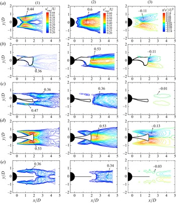


 Open access