


1. Introduction
Particle-laden turbulent flows have attracted the attention of many scholars over the last decades because of their relevance, which goes beyond a fundamental interest and encompasses several applications in natural, industrial and geophysical fields (De Lillo et al. Reference De Lillo, Cencini, Durham, Barry, Stocker, Climent and Boffetta2014; Breard et al. Reference Breard, Lube, Jones, Dufek, Cronin, Valentine and Moebis2016; Sengupta, Carrara & Stocker Reference Sengupta, Carrara and Stocker2017; Falkinhoff et al. Reference Falkinhoff, Obligado, Bourgoin and Mininni2020).
The inclusion of solid particles in the flow introduces additional momentum in the suspension that may result in modulation of the flow structures. When the suspension is dilute enough, the carrier flow is almost not altered by the presence of the particles. When the suspension is non-dilute, instead, the carrier flow undergoes macroscopic changes, and the particle–fluid interaction cannot be neglected (Balachandar & Eaton Reference Balachandar and Eaton2010; Brandt & Coletti Reference Brandt and Coletti2022).
The rheological properties of suspensions have been first studied in the limit of the viscous Stokesian regime, where the inertial effects are negligible. The presence of the particles affects the deformation of the surrounding fluid, and the effective viscosity  $\mu _e$ of the particle–fluid mixture depends on the dynamics of the dispersed phase. For a dilute suspension with negligible inter-particle interactions, Einstein (Reference Einstein1906) derived an analytical linear relation for the effective viscosity, i.e. $\mu _e = \mu (1+2.5\varPhi _V)$, with $\varPhi _V = V_p/(V_p + V_f)$ being the volume fraction of the dispersed phase; $V_p$ and $V_f$ are the volumes of the solid and fluid phases. Later, a quadratic correction was proposed by Batchelor (Reference Batchelor1970) and Batchelor & Green (Reference Batchelor and Green1972) to account for mutual particle interaction for slightly higher volume fractions. For higher concentrations, where the inter-particle interactions play a crucial role, only semi-empirical formulas exist (Krieger & Dougherty Reference Krieger and Dougherty1959).
In the turbulent regime, the particle size has been found to play a crucial role in determining the effect of the dispersed phase on the carrier flow. Gore & Crowe (Reference Gore and Crowe1989) considered data from both particulate turbulent pipe flows and jets, and found that the turbulence modulation depends on the ratio of the particle diameter  $D$ and the flow integral scale $\mathcal {L}$. When $D/\mathcal {L}>0.1$ the turbulent intensity of the carrier phase increases with respect to the single-phase case, while when $D/\mathcal {L}<0.1$ it decreases. Large particles produce fluctuations in their wake and enhance the turbulent activity, while small ones drain energy from the large-scale turbulent eddies of the flow. Indeed, Tsuji & Morikawa (Reference Tsuji and Morikawa1982) experimentally considered an air–solid two-phase flow in a horizontal pipe with diameter of $30\,\mathrm {mm}$, and investigated the influence of small and large particles with diameter of $0.2\,\mathrm {mm}$ and $3.4\,\mathrm {mm}$ on the carrier flow, varying the section-average air velocity between $6$ and $20\,\mathrm {m}\,\mathrm {s}^{-1}$. They observed that large particles markedly increase the turbulent activity, while small ones reduce it. These results were later confirmed by the same authors, with experiments of an air–solid two-phase flow in a vertical pipe (Tsuji, Morikawa & Shiomi Reference Tsuji, Morikawa and Shiomi1984). More recently, Hoque et al. (Reference Hoque, Mitra, Sathe, Joshi and Evans2016) studied the turbulence modulation of a nearly isotropic flow field due to the presence of single glass particles with varying diameter, and observed that the critical ratio of the particle size to integral scale of $D/\mathcal {L} = 0.41$ separates the regimes of attenuation and enhancement of turbulent intensity.
Large steps towards a complete description of the interaction between rigid particles of different size and density and the fluid phase have been performed over the last years thanks to the increase in supercomputers’ power, which enables the study of such problem via direct numerical simulations (DNS) (Crowe, Troutt & Chung Reference Crowe, Troutt and Chung1996; Burton & Eaton Reference Burton and Eaton2005; Maxey Reference Maxey2017). One of the most common approaches used today to model many particle-laden flows is based on the point-particle approximation. In general, each particle is treated as a mathematical point source of mass, momentum and energy, with the particles assumed to be much smaller than any structure of the flow. The point-particle approximation is valid in the limit in which the volume of each particle is negligible, i.e. the case with vanishing disperse-phase volume fraction. Indeed, the point-particle assumption requires that the fluid velocity field does not display a turbulent behaviour at the scale of the particle, meaning that  $D \le \eta$ ( $\eta$ being the Kolmogorov scale). According to this method, the fluid–solid interaction is completely described by a forcing term that should be accurately modelled; see for example Maxey & Riley (Reference Maxey and Riley1983). The theoretical developments of the point-particle approximation, however, are limited to a relatively narrow range of parameters. For example, investigating the motion of a single particle in homogeneous isotropic turbulence, Homann & Bec (Reference Homann and Bec2010) found that the particle velocity variance reflects what predicted by the point-particle approximation for $D/ \eta \le 4$ only. Within the point-particle approximation, Elghobashi & Truesdell (Reference Elghobashi and Truesdell1993) and Elghobashi (Reference Elghobashi1994) showed the importance of the particle Stokes number in determining the turbulence modulation. Costa, Brandt & Picano (Reference Costa, Brandt and Picano2020) tested the point-particle approximation in a turbulent channel flow laden with small inertial particle, with high particle-to-fluid density ratio. They considered a volume fraction of $\varPhi _V \approx 10^{-5}$ to ensure that the particle feedback on the flow is negligible, and discussed the validity of models that approximate the particle dynamics considering only the inertial and nonlinear drag forces. They observed that in the bulk of the channel these models predict pretty well the statistics of the particle velocity. Close to the wall, however, the models fail as they are not able to capture the shear-induced lift force acting on the particles in this region, which instead is well predicted by the lift force model introduced by Saffman (Reference Saffman1965).
A complete understanding of the fluid–solid interaction problem over a wider range of parameters ( $D/\eta \gtrsim 1$, $\varPhi _V \gtrsim 10^{-4}$ and particle-to-fluid density ratio $\rho _p/\rho _f \gtrsim 10$; see Brandt & Coletti Reference Brandt and Coletti2022) requires us to properly resolve the flow around each particle, without the need to rely on models. In this respect, over the last years, several numerical methods based on the coupling between DNS and the immersed boundary method (IBM) have appeared, and have been used to study particulate turbulence; see for example the numerical methods described in Kajishima et al. (Reference Kajishima, Takiguchi, Hamasaki and Miyake2001), Uhlmann (Reference Uhlmann2005), Huang, Shin & Sung (Reference Huang, Shin and Sung2007), Breugem (Reference Breugem2012), Kempe & Fröhlich (Reference Kempe and Fröhlich2012) and Hori, Rosti & Takagi (Reference Hori, Rosti and Takagi2022). Based on these developments, several works have carried out DNS of particulate turbulence, but mainly considering small Reynolds numbers and/or large particles, due to the extremely large computational cost; see for example Lucci, Ferrante & Elghobashi (Reference Lucci, Ferrante and Elghobashi2010, Reference Lucci, Ferrante and Elghobashi2011); Oka & Goto (Reference Oka and Goto2022) for homogeneous isotropic turbulence, Uhlmann (Reference Uhlmann2008); Shao, Wu & Yu (Reference Shao, Wu and Yu2012); Wang, Abbas & Climent (Reference Wang, Abbas and Climent2018); Peng, Ayala & Wang (Reference Peng, Ayala and Wang2019); Rosti & Brandt (Reference Rosti and Brandt2020); Yousefi, Ardekani & Brandt (Reference Yousefi, Ardekani and Brandt2020); Costa, Brandt & Picano (Reference Costa, Brandt and Picano2021) and Gao, Samtaney & Richter (Reference Gao, Samtaney and Richter2023) for channel flow, Lin et al. (Reference Lin, Yu, Shao and Wang2017) for duct flow and Wang et al. (Reference Wang, Peng, Guo and Yu2016) and Zahtila et al. (Reference Zahtila, Chan, Ooi and Philip2023) for pipe flow.
In this work, we consider non-dilute suspensions of finite-size spherical particles in periodic turbulence, and investigate the fluid–solid interaction in the two-dimensional parameter space of particle size and density. This flow configuration has been investigated by several authors over the years. Ten Cate et al. (Reference Ten Cate, Derksen, Portela and van Den Akker2004) investigated the influence of suspensions of finite-size particles with a solid-to-fluid density ratio of  $\rho _p/\rho _f \approx 1.5$ and $\varPhi _V \approx 0.02\unicode{x2013}0.1$ on periodic turbulence at a microscale Reynolds number of $Re_\lambda = u' \lambda / \nu = 61$ ( $u'$ is the average velocity fluctuation, $\lambda$ is the Taylor length scale and $\nu$ is the fluid kinematic viscosity). They found that the energy spectrum is enhanced for wavenumbers $\kappa >\kappa _p\approx 0.72 \kappa _d$, where $\kappa _d = 2 {\rm \pi}/D$ is the wavenumber corresponding to the particle diameter, and that it is attenuated for $\kappa <\kappa _p$. The particles drain energy from the large scales of the flow, and inject it at smaller scales by means of their wake. Hwang & Eaton (Reference Hwang and Eaton2006) experimentally studied the influence of heavy particles with a diameter similar to the Kolmogorov scale on homogeneous isotropic turbulence, setting the Reynolds number at $Re_\lambda =230$. They observed that the fluid turbulent kinetic energy and the viscous dissipation decrease when increasing the mass loading. Yeo et al. (Reference Yeo, Dong, Climent and Maxey2010) numerically confirmed the results by Ten Cate et al. (Reference Ten Cate, Derksen, Portela and van Den Akker2004) at $Re_\lambda \approx 60$ with a particle-to-fluid density ratio of $\rho _p/\rho _f = 1.4$ and a volume fraction of $\varPhi _V = 0.06$. Lucci et al. (Reference Lucci, Ferrante and Elghobashi2010) studied the influence of particles of Taylor length scale on decaying isotropic turbulence. They found that, in contrast to what happens when using particles with diameter smaller than the Kolmogorov scale, the turbulent kinetic energy is always smaller than that of the single-phase flow, and that the two-way coupling rate of change is always positive. Later, using the same framework, Lucci et al. (Reference Lucci, Ferrante and Elghobashi2011) found that the Stokes number should not be used as an indicator to estimate at which extent particles of the Taylor length scale modulate the turbulent carrier flow, as particles with same response time but different diameter or density may have different effect on the flow, unlike what observed for sub-Kolmogorov particles (Ferrante & Elghobashi Reference Ferrante and Elghobashi2003; Yang & Shy Reference Yang and Shy2005). Uhlmann & Chouippe (Reference Uhlmann and Chouippe2017) investigated the influence of spherical particles with diameter of approximately $5$ and $8$ times the Kolmogorov length and particle-to-fluid density ratio of $\rho _p/\rho _f=1.5$ on forced homogeneous isotropic turbulence at $Re_\lambda \approx 130$. They observed that the disperse phase exhibits clustering with moderate intensity, and that this clustering decreases with the particle diameter. They also suggest that small and light finite-size particles follow the expansive directions of the fluid acceleration field, as happens also for sub-Kolmogorov particles (Chen, Goto & Vassilicos Reference Chen, Goto and Vassilicos2006; Goto & Vassilicos Reference Goto and Vassilicos2008). More recently, Olivieri, Cannon & Rosti (Reference Olivieri, Cannon and Rosti2022) considered homogeneous isotropic turbulence with a well developed inertial range of scales (they set the Reynolds number at $Re_{\lambda } \approx 400$), and investigated the turbulence modulation by non-dilute suspensions ( $\varPhi _V=0.079$) of spherical particles with size that lies in the inertial range ( $D/\eta =123$), varying the particle-to-fluid density ratio in the range $1.3 \le \rho _p/\rho _f \le 100$. They characterised how particles modify the classical energy cascade described by Richardson and Kolmogorov. Olivieri, Cannon & Rosti (Reference Olivieri, Cannon and Rosti2022) observed that the energy transfer is governed by the fluid–solid coupling at scales larger than the particle diameter, and that the classical energy cascade is recovered only at smaller scales. Oka & Goto (Reference Oka and Goto2022) performed a parametric DNS study of particulate homogeneous isotropic turbulence, and investigated the turbulence modulation due to spherical solid particles with different Stokes number at a volume fraction of $\varPhi _V = 8.1 \times 10^{-3}$ and reference Reynolds number of $Re_\lambda \le 100$. They varied the particle diameter in the $7.8 \le D/\eta \le 64$ range, and found that the turbulent kinetic energy decreases when reducing $D$, due to the additional energy dissipation rate in the wake. Similarly, Shen et al. (Reference Shen, Peng, Wu, Chong, Lu and Wang2022) used a multiple-relaxation-time lattice Boltzmann model, and studied the influence of the particle-to-fluid density ratio and particle diameter on the turbulence modulation at $Re_\lambda \approx 75$, varying the parameters in the ranges $8 \le D/\eta \le 16$ and $5 \le \rho _p/\rho _f \le 20$. Besides confirming the turbulent kinetic attenuation for smaller and heavier particles, they observed that the region affected by the particles depends on their diameter, and that the dissipation close to their surfaces increases with the particle density due to the larger slip velocity and particle Reynolds number.
Despite the large number of studies in the literature, further investigations are necessary for a complete understanding of particle-laden turbulent flows, even in the simple framework of a triperiodic box. Most of the numerical works, indeed, have considered relatively low Reynolds numbers, where the inertial range of turbulence is not completely developed, and relatively low volume fractions, that lead to a rather weak flow modulation (see figure 1). As reported in Brandt & Coletti (Reference Brandt and Coletti2022), reliable studies at larger Reynolds numbers and at higher concentrations are needed, to bridge the gap between the studies of small, heavy particles and large, weakly buoyant particles, and to promote the development of models that go beyond the point-particle approximation. In this work, we take a step in this direction. By means of a massive parametric study based on DNS and IBM, we investigate the fluid–solid interaction in a triperiodic turbulent flow laden with spherical particles with a size that lies within the inertial range. We consider a Reynolds number of  $Re_\lambda \approx 400$, which ensures an extensive inertial range of scales, and a volume fraction of $\varPhi _V = 0.079$, which is large enough for the suspension to be non-dilute, but small enough for the particle–particle interactions to be subdominant; see figure 1. The fluid–solid interaction is studied in the two-dimensional parameter space of particle size $D$ and particle-to-fluid density ratio $\rho _p/\rho _f$. The particle size is varied in the range $16 \le D/\eta \le 123$, while the particle density is varied in the range $1.3 \le \rho _p/\rho _f \le 100$. The specific goals of the paper are: (i) to provide an extensive characterisation of the carrier flow modulation in the $D-\rho _p/\rho _f$ space, extending the previous works by Olivieri et al. (Reference Olivieri, Cannon and Rosti2022) and Oka & Goto (Reference Oka and Goto2022) to a wider range of parameters and to a larger Reynolds number; (ii) to describe the near-particle flow modulation and provide insights into how the fluid–solid interaction changes with $D$ and $\rho _p/\rho _f$, which is relevant for modelling purposes; (iii) to investigate the collective motion and preferential location of the particles, extending the work by Uhlmann & Chouippe (Reference Uhlmann and Chouippe2017) to larger and heavier particles and to a larger Reynolds number.

Figure 1. Comparison between the values of the Reynolds number  $Re_\lambda$, the particle size $D/\eta$ and the volume fraction $\varPhi _V$ of the suspension considered in previous works in the literature and the ones considered in the present work. This list considers only recent numerical works and is not intended to be exhaustive.
The paper is structured as follows. In § 2, the physical model and the numerical method are briefly presented. Section 3 describes the influence of the solid phase on the carrier flow. In § 4, the effect of the particle size and density on the near-particle flow modulation is addressed. The dynamics of the particles and their collective motion are then discussed in § 5. Eventually, in § 6 concluding remarks are provided.
2. Numerical methods
The fluid–solid interaction of non-dilute suspension of solid spherical particles is investigated by means of a massive parametric study based on DNS. We consider an ensemble of  $N$ finite-size spherical particles with size $D$ and density $\rho _p$, suspended in a periodic turbulent flow; see figure 2. Particles are released in a cubic domain of size $L=2{\rm \pi}$, having periodic boundary conditions in all directions, where turbulence is generated and sustained using the Arnold–Beltrami–Childress (ABC) cellular-flow forcing (Podvigina & Pouquet Reference Podvigina and Pouquet1994).

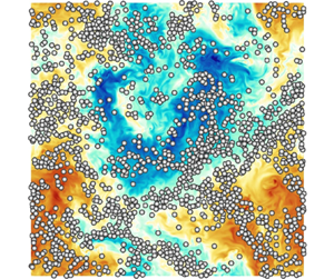
Figure 2. Instantaneous velocity field and particles in a two-dimensional plane for the  $D/\eta =16$ and $D/\eta =123$ particulate cases with mass fraction $M=0.3$.
The carrier flow is governed by the incompressible Navier–Stokes equations for a Newtonian fluid, i.e.
 \begin{equation} \begin{cases} \dfrac{\partial \boldsymbol{u}}{\partial t} + \boldsymbol{\nabla} \boldsymbol{\cdot} \boldsymbol{u} \boldsymbol{u} ={-}\dfrac{1}{\rho_f} \boldsymbol{\nabla} p + \nu \nabla^2 \boldsymbol{u} + \boldsymbol{f} + \boldsymbol{f}^{\leftarrow p} \\ \boldsymbol{\nabla} \boldsymbol{\cdot} \boldsymbol{u} = 0. \end{cases} \end{equation}
Here,  $\boldsymbol {u}=(u,v,w)$ is the velocity vector field, $p$ is the reduced pressure and $\rho _f$ and $\nu$ are the fluid density and kinematic viscosity. In the momentum equation, the term $\boldsymbol {f}^{\leftarrow p}$ is the force due to the solid phase, and $\boldsymbol {f}$ is the external ABC body force used to sustain turbulence
 \begin{align}
\boldsymbol{f}=\left(\frac{2{\rm \pi}}{L}\right)^2 F_o
\begin{pmatrix} A \sin\left(\dfrac{2{\rm \pi}}{L}z\right) + C
\cos\left(\dfrac{2{\rm \pi}}{L}y\right) \\ B
\sin\left(\dfrac{2{\rm \pi}}{L}x\right) + A
\cos\left(\dfrac{2{\rm \pi}}{L}z\right) \\ C
\sin\left(\dfrac{2{\rm \pi}}{L}y\right) + B
\cos\left(\dfrac{2{\rm \pi}}{L}x\right) \end{pmatrix},
\end{align}
\begin{align}
\boldsymbol{f}=\left(\frac{2{\rm \pi}}{L}\right)^2 F_o
\begin{pmatrix} A \sin\left(\dfrac{2{\rm \pi}}{L}z\right) + C
\cos\left(\dfrac{2{\rm \pi}}{L}y\right) \\ B
\sin\left(\dfrac{2{\rm \pi}}{L}x\right) + A
\cos\left(\dfrac{2{\rm \pi}}{L}z\right) \\ C
\sin\left(\dfrac{2{\rm \pi}}{L}y\right) + B
\cos\left(\dfrac{2{\rm \pi}}{L}x\right) \end{pmatrix},
\end{align}
where  $A=B=C=1$, and $F_o$ is a constant parameter. The dynamics of the spherical particles is governed by the Euler–Newton equations
 \begin{equation} \begin{cases} m
\dfrac{\text{d} \boldsymbol{u}_p}{\text{d} t} =
\boldsymbol{f}^{\leftarrow f} +
\boldsymbol{f}^{\leftrightarrow p} \\ I \dfrac{\text{d}
\boldsymbol{\omega}_p}{\text{d} t} =
\boldsymbol{L}_p^{\leftarrow f}, \end{cases}
\end{equation}
\begin{equation} \begin{cases} m
\dfrac{\text{d} \boldsymbol{u}_p}{\text{d} t} =
\boldsymbol{f}^{\leftarrow f} +
\boldsymbol{f}^{\leftrightarrow p} \\ I \dfrac{\text{d}
\boldsymbol{\omega}_p}{\text{d} t} =
\boldsymbol{L}_p^{\leftarrow f}, \end{cases}
\end{equation}
where  $\boldsymbol {u}_p$ and $\boldsymbol {\omega }_p$ are the velocity and angular velocity of the particles, and $m={\rm \pi} \rho _p D^3/6$ and $I = m D^2/10$ are the mass and inertial moment of the particles. Also, $\boldsymbol {f}^{\leftarrow f}$ is the force due to the fluid and $\boldsymbol {f}^{\leftrightarrow p}$ is the force due to the interaction between particles. In this study gravitational forces are not considered.
We set  $\rho _f=1$, $\nu =1/400$ and $F_o=5$ to achieve in the single-phase case a micro-scale Reynolds number of $Re_\lambda = u' \lambda / \nu \approx 435$, ( $u'$ is the root mean square of the velocity fluctuations and $\lambda$ is the Taylor length scale), which ensures an extensive inertial range of scales. The particle diameter $D$ is varied in the range $16 \le D/\eta \le 123$ ( $\eta$ is the Kolmogorov length scale for the single-phase case). The number $N$ of particles is increased as the diameter decreases, to maintain the volume fraction $\varPhi _V = V_p/(V_p + V_f)$ constant to a value of $\varPhi _V = 0.0792$, as in Olivieri et al. (Reference Olivieri, Cannon and Rosti2022). The particle density $\rho _p$ is varied in the range $1.29 \le \rho _p/\rho _f \le 104.7$ to consider both light and heavy particles, corresponding to a variation of the mass fraction $M = \rho _p V_p / (\rho _f V_f + \rho _p V_p)$ in the range $0.1 \le M \le 0.9$. The smallest value of $\rho _p/\rho _f=1.29$ and the largest value of $\rho _p/\rho _f = 104.7$ have been chosen based on the results of Olivieri et al. (Reference Olivieri, Cannon and Rosti2022). As shown in figures 2 and 3 of their paper, indeed, the flow modulation only marginally changes when further increasing the density ratio $\rho _p/\rho _f$.
The governing equations are numerically integrated in time using the in-house solver Fujin (https://groups.oist.jp/cffu/code), which is based on an incremental pressure-correction scheme. It considers the Navier–Stokes equations written in primitive variables on a staggered grid, and uses second-order finite differences in all the directions. The Adams–Bashforth time scheme is used for advancing the momentum equation in time. The Poisson equation for the pressure enforcing the incompressibility constraint is solved using a fast and efficient approach based on the fast Fourier transform. The solver is parallelised and is based on a Cartesian block decomposition of the domain in the  $x$ and $y$ directions, and uses the message passing interface library for maximum portability. The governing equations for the particles are dealt with via the IBM introduced by Hori et al. (Reference Hori, Rosti and Takagi2022). The fluid–solid coupling is achieved in an Eulerian framework (Kajishima et al. Reference Kajishima, Takiguchi, Hamasaki and Miyake2001), and accounts for the inertia of the fictitious fluid inside the solid phase, to properly reproduce the behaviour of the particles in both the neutrally buoyant case and in the presence of a density difference between the fluid and solid phases. The soft sphere collision model, first proposed by Tsuji, Kawaguchi & Tanaka (Reference Tsuji, Kawaguchi and Tanaka1993), is used to prevent the interpenetration between particles. A fixed-radius near-neighbours algorithm (see Monti et al. (Reference Monti, Rathee, Shen and Rosti2021) and references therein) is used for the particle interaction to avoid an otherwise prohibitive increase of the computational cost when the number of particles increases.
The fluid domain is discretised using  $N_{point}=1024$ points in the three directions, to ensure that all the scales down to the smallest dissipative (Kolmogorov) ones are solved, leading to $\eta /\Delta x= O(1)$, where $\Delta x$ denotes the grid spacing. At the initial time the particles are randomly distributed within the domain. Excluding the initial transient period needed to reach the statistically steady state, all simulations are advanced for approximately $15T$, where $T=L/\overline {u'}$ is the turnover time of the largest eddies. For the particle-laden cases with $D/\eta =32$, the simulations have been advanced for a longer period, i.e. approximately $35T$, to ensure convergence of the temporal averages discussed in § 3. Note that the particle-laden cases with $D/\eta =123$ are the same considered in Olivieri et al. (Reference Olivieri, Cannon and Rosti2022). Details of the numerical simulations are provided in table 1. The adequacy of the grid resolution is assessed in Appendix B.
Table 1. Details of the numerical simulations considered in the present parametric study:  $M$ is the mass fraction; $\rho _p/\rho _f$ is the particle-to-fluid density ratio; $N$ is the number of particles; $D$ is the particle diameter; $\lambda$ is the Taylor length scale; $\eta$ is the Kolmogorov scale; $E$ is the fluid kinetic energy; $\epsilon$ is the dissipation; $Re_\lambda$ is the Reynolds number based on $u'=\sqrt {2E/3}$ and on the Taylor length scale; $St$ is the Stokes number defined as $St=\tau _p/\tau _f$, where $\tau _p=(\rho _p/\rho _f)D^2/(18 \nu )$ is the relaxation time of the particle velocity and $\tau _f=\mathcal {L}/\sqrt {2\bar {\!\langle {E}\rangle \!}/3}$ is the turnover time of the largest eddies; $\mathcal {L}={\rm \pi} /(4\bar {\!\langle {E}\rangle \!}/3)\int _0^\infty \mathcal {E}(\kappa )/\kappa \,\text {d} \kappa$ is the fluid integral scale and $\mathcal {E}$ is the energy spectrum.

To demonstrate the independence of the results from the external forcing, additional simulations have been carried out using the forcing introduced by Eswaran & Pope (Reference Eswaran and Pope1988) to sustain turbulence; see Appendix A. Unlike the ABC forcing, indeed, the Eswaran & Pope forcing has a random component, and does not generate an inhomogeneous shear at the largest scales. As shown in § 3 and in Appendix A, the effect of the solid phase on the largest and energetic scales of the flow changes with the kind of forcing considered. At smaller scales, however, the results do not depend on the external forcing. At small scales the flow modulation does not depend on how energy is injected in the system, and the effect of the solid phase is substantially the same for the two considered forcings.
3. The carrier flow
3.1. Integral quantities
In this section we investigate the influence of the particles on the fluid phase. Figure 3 shows the dependence of the fluid average kinetic energy  $\overline {\!\langle {E (\boldsymbol {x},t) }\rangle \! }$ on $M$ and $D$. We define the fluid kinetic energy as
 \begin{equation} E(t) = \tfrac{1}{2} | \boldsymbol{u}(\boldsymbol{x},t) - \!\langle {\boldsymbol{U}(\boldsymbol{x})}\rangle \!|^2, \end{equation}
while  $\bar {\cdot }$ and $\!\langle {\cdot }\rangle \!$ indicate average in time and along the homogeneous directions respectively; $\boldsymbol {U}(\boldsymbol {x}) \equiv \overline { \boldsymbol {u}( \boldsymbol {x},t) }$ is the three-dimensional fluid velocity field averaged in time. As discussed by Chiarini, Cannon & Rosti (Reference Chiarini, Cannon and Rosti2024), due to the presence of the inhomogeneous mean shear induced by the external ABC forcing, the dispersed phase modulates the largest scales of the carrier flow in a way that substantially changes with the size and density of the particles. Similarly to what found by previous authors (Oka & Goto Reference Oka and Goto2022; Peng, Sun & Wang Reference Peng, Sun and Wang2023), for large and/or light particles, i.e. $D/\eta > 64$ and/or $M < 0.45$, the kinetic energy $\!\langle {\bar {E}}\rangle \!$ of the carrier flow monotonically decreases when the mass fraction increases and/or the particle size decreases; we call this regime A in figure 3. When fixing $D$, indeed, an increase of the density of the particles leads to an increase of the inertia of the fluid–particle system, and the same large-scale external forcing generates weaker fluctuations. When fixing $M$, instead, smaller particles are more effective in attenuating the fluid velocity fluctuations. A decrease of $D$ corresponds to an increase of the total solid surface area and, therefore, to an increase of the high dissipation rate regions that form around the particles (see § 4). On the other hand, when particles are smaller and heavier, i.e. $D/\eta \le 64$ and $M \gtrapprox 0.45$, the scenario changes: the kinetic energy $\!\langle {\bar {E}}\rangle \!$ sharply increases, and does not have a monotonic dependence on $D$ and $M$. This is what we call regime B in figure 3. The value of $M$ that delimits regimes A and B increases when the particle size decreases, suggesting that the occurrence of regime B is mainly driven by the inertia of the single particles. Note that, for $D/\eta =32$ and $0.45 \le M \le 0.6$ and $D/\eta =64$ and $M=0.45$, the presence of the solid phase enhances the total fluid energy compared with the single-phase case.

Figure 3. Dependence of the average energy of the fluid phase  $\bar {\!\langle {E}\rangle \!}$ on the density and size of the particles. Here, $\overline {\!\langle {E_0}\rangle \!}$ refers to the single-phase case. Circles refer to regime A and diamonds to regime B (see text).
In this work, regimes A (circles in figure 3) and B (squares in figure 3) are only briefly described; we refer the interested reader to Chiarini et al. (Reference Chiarini, Cannon and Rosti2024) for more details. To characterise the two regimes, we use the temporal average operator and isolate the influence of the dispersed phase on the largest and smaller scales of the flow. We focus on  $D/\eta =32$, being the case that shows the strongest flow modulation, and for which $\!\langle {\bar {E}}\rangle \!$ undergoes the maximum enhancement. We decompose the complete velocity field $\boldsymbol {u}(\boldsymbol {x},t)$ into its temporal mean field $\boldsymbol {U}(\boldsymbol {x})$ and the fluctuating field $\boldsymbol {u}'(\boldsymbol {x},t) = \boldsymbol {u}(\boldsymbol {x},t) - \boldsymbol {U}(\boldsymbol {x})$, and plot the variances of their three components in figure 4. Light particles (regime A) influence the flow without introducing a preferential direction, modulating both the mean and fluctuating fields in a isotropic way: here, $\!\langle {UU}\rangle \! \approx \!\langle {VV}\rangle \! \approx \!\langle {WW}\rangle \!$ and $\!\langle {u'u'}\rangle \! \approx \!\langle {v'v'}\rangle \! \approx \!\langle {w'w'}\rangle \!$. Heavy particles (regime B), instead, modulate differently the largest and smaller scales of the flow. They attenuate the fluctuating field (i.e. the smaller scales of the flow) in a isotropic way, but modulate the mean-flow field (i.e. the largest scales of the flow) towards a more energetic and anisotropic state. In this case, the presence of the dispersed phase enhances two components of the mean flow ( $U$ and $V$) and attenuates the third one ( $W$). Here, $\!\langle {UU}\rangle \! \approx \!\langle {VV}\rangle \! \gg \!\langle {WW}\rangle \!$ and $\!\langle {u'u'}\rangle \! \approx \!\langle {v'v'}\rangle \! \approx \!\langle {w'w'}\rangle \!$. The increase of the total fluid energy $\!\langle {\bar {E}}\rangle \!$ observed in figure 3 for $0.45 \le M \le 0.6$ is entirely due to the enhanced mean-flow contribution. In regime B the scenario is the following. Due to their large inertia, particles are not able to follow the inhomogeneous mean shear generated by the ABC forcing, and deviate towards almost straight trajectories that lie in the $x-y$ plane (see § 5.1), showing anomalous transport. In doing this, they modulate the flow towards an anisotropic and almost two-dimensional state. Here, the mean-flow velocity components that lie in the plane of the trajectories of the particles ( $U$ and $V$) are enhanced, while the out-of-plane component ( $W$) is attenuated. As detailed in Chiarini et al. (Reference Chiarini, Cannon and Rosti2024), this anisotropic modulation of the largest scales is due to the interaction of the particle with the inhomogeneous mean shear induced by the ABC forcing. When the inhomogeneous mean shear is not present, the anisotropic modulation of the largest scales is not observed; see Appendix A.

Figure 4. Dependence of the (a) mean and (b) fluctuating energy on the mass fraction for the  $D/\eta =32$ particle-laden case.
Note that, when presenting the results, we deliberately choose a reference system such that, for all cases, the  $z$ axis is aligned with the mostly attenuated mean-flow velocity component, similarly to what is done in Chiarini et al. (Reference Chiarini, Cannon and Rosti2024). In the reference system of the simulation, however, the direction aligned with the attenuated mean-flow velocity component changes with the initial condition.
3.2. Mean-flow modulation
Figure 5 plots in the  $x=L/2$ plane the three components of the mean-flow velocity field, i.e. (a,d,g) $U$, (b,e,h) $V$ and (c,f,i) $W$, for (a–c) the single-phase case, and for the $D/\eta =32$ particulate cases with (d–f) $M=0.3$ and (g–i) $M=0.6$. In the single-phase case, the mean flow resembles the laminar ABC profile, i.e. $(U,V,W) \approx (A \sin (z) + C \cos (y), B \sin (x) + A \cos (z), C \sin (y) + B \cos (x))$ with $A=B=C=1$, similarly to what was observed for the Kolmogorov flow by other authors (Borue & Orszag Reference Borue and Orszag1996); note for example the cellular pattern in the map of $U$. In the particle-laden case with $M=0.3$ (regime A), the mean flow retains a similar pattern, in agreement with the isotropic and marginal mean-flow modulation observed in figure 4. In regime B, instead, the structure of the mean flow changes; for $M=0.6$, figure 5 shows that the $U$ and $V$ velocity components are strongly enhanced, while the $W$ component is attenuated. Moreover, the mean flow does not show the ABC cellular pattern anymore (see the $U$ velocity component): the dependence on $x$ and $y$ is almost lost, while the sinusoidal dependence on $z$ is retained, i.e. $(U,V,W) \approx (\sin (z),\cos (z),0)$ (see Chiarini et al. (Reference Chiarini, Cannon and Rosti2024) for further details).

Figure 5. Mean-flow velocity components on the  $x=L/2$ plane; (a,d,g) $U$, (b,e,h) $V$, (c,f,i) $W$. (a–c) Single phase, (d–f) $D/\eta =32$ and $M=0.3$, (g–i) $D/\eta =32$ and $M=0.6$.
For a quantitative description of the mean-flow modulation, figure 6 shows the histogram of the spatial distribution of the three velocity components  $U(\boldsymbol {x})$, $V(\boldsymbol {x})$ and $W(\boldsymbol {x})$ for the $D/\eta =32$ particle-laden cases. Recall that $\boldsymbol {U}(\boldsymbol {x}) \equiv \overline {\boldsymbol {u}(\boldsymbol {x},t) }$ is the space-dependent fluid velocity field averaged in time. In regime A ( $M < 0.45$) the modulation of $\boldsymbol {U}(\boldsymbol {x})$ is isotropic and the distributions of the three velocity components almost overlap, showing a unimodal distribution centred on $\hat {U} = \hat {V} = \hat {W} = 0$. In regime B ( $M \ge 0.45$), the $W$ component retains a similar unimodal distribution, but the distribution becomes narrower, in agreement with the progressive attenuation of its spatial fluctuations. In agreement with the spatial distribution shown in figure 5, instead, the $U$ and $V$ velocity components show a symmetric bimodal distribution. The modes $\pm \hat {U} = \pm \hat {V}$ change with $M$, and can be used as an estimate of the mean-flow anisotropy; see figure 6(e).

Figure 6. Time-average flow velocity  $\boldsymbol {U}(\boldsymbol {x})$ for $D/\eta =32$. Histogram of the spatial distribution of the three components of $\boldsymbol {U}(\boldsymbol {x})$ for the single phase (a) and the $D/\eta =32$ particulate cases with $M=0.3$ (b), $M=0.6$ (c) and $M=0.9$ (d). Black is for $U$, green for $V$ and orange for $W$. (e) Shows the dependence of the modes of the three velocity components ( $\hat {U}$, $\hat {W}$ and $\hat {W}$) on $M$.
$M$.
3.3. Turbulence modulation
3.3.1. Energy spectra
To shed light on the mechanism with which the particles modulate the flow at smaller scales, we investigate the influence of the solid phase on the scale-by-scale energy content of the carrier flow, i.e. the energy spectrum.
It is worth recalling that, although for some  $M$ and $D$ the solid phase modulates the largest scales ( $\kappa /\kappa _L=1$, where $\kappa$ is the wavenumber and $\kappa _L = 2 {\rm \pi}/L$) towards an anisotropic state (regime B), smaller scales with $\kappa /\kappa _L>1$ are isotropic and homogeneous for all cases (see figure 4). The flow modulation for $\kappa /\kappa _L>1$, indeed, does not depend on how energy is injected in the system, or on how particles modify the structure of the largest scales. This is clearly shown in Appendix A, where we present results from additional simulations carried out using the forcing introduced by Eswaran & Pope (Reference Eswaran and Pope1988) that, unlike the ABC forcing, does not generate a coherent and inhomogeneous shear at the largest scales $\kappa /\kappa _L=1$.
The presence of the solid phase modifies the energy spectrum of the carrier flow in a way that largely depends on the size and density of the particles. As first observed by Ten Cate et al. (Reference Ten Cate, Derksen, Portela and van Den Akker2004), particles drain energy from the fluid phase at scales larger than  $D$, and inject it back into the fluid at smaller scales by means of their wake. This results into an energy depletion at low wavenumbers, i.e. large scales, and energy enhancement at large wavenumbers, i.e. small scales. Figures 7 and 8 consider separately the effect of the particle size and density on the energy spectrum. Note in passing that the single-phase energy spectrum (black line) shows that the Reynolds number considered in this work leads to a proper separation of scales, with an inertial range of scales that extends to almost two decades of wavenumbers. Also, the oscillations at large wavenumbers appear as we compute the spectra using the fluid velocity field at all the mesh points of the computational domain, including those that are inside the particles (Lucci et al. Reference Lucci, Ferrante and Elghobashi2010). However, when dealing with structure functions in the real space (see § 3.3.3), we have verified that the results do not change when the points within the particles are neglected.

Figure 7. Dependence of the energy spectrum on the particles size  $D/\eta$ for (a) $M=0.6$ and (b) $M=0.9$. The circles identify the particle diameter wavenumbers $\kappa _d = 2 {\rm \pi}/D$. Here and hereinafter, $\kappa _L = 2 {\rm \pi}/L$.

Figure 8. Dependence of the energy spectrum on the mass fraction for (a)  $D/\eta =123$ and (b) $D/\eta =32$. The circles identify the particle diameter wavenumbers $\kappa _d = 2 {\rm \pi}/D$.
We start investigating the dependence of the energy spectrum on the particle size (figure 7). For large particles, the energy depletion is limited at the largest scales  $\kappa < \kappa _{p,1} \lessapprox \kappa _d = 2 {\rm \pi}/D$, the energy spectrum recovers the $\kappa ^{-5/3}$ decay predicted by the Kolmogorov theory for intermediate $\kappa$ and energy is enhanced at the smallest scales $\kappa > \kappa _{p,2}$. For example, for $D/\eta =123$ the energy depletion is observed for $\kappa /\kappa _L \le \kappa _{p,1}/\kappa _L \approx 5$, while energy enhancement occurs for $\kappa /\kappa _L \ge \kappa _{p,2}/\kappa _L \approx 230$. Smaller particles amplify the overall mechanism. They drain energy from a wider range of scales, and, therefore, inject back a larger amount of energy at a wider range of small scales. For smaller particles, indeed, $\kappa _{p,1}$ increases, while $\kappa _{p,2}$ decreases. For $M=0.6$, for example, we measure that $\kappa _{p,1}/\kappa _L \approx 49, 25, 17$ and $8$ and $\kappa _{p,2}/\kappa _L \approx 189, 199, 219$ and $230$ for $D/\eta =16, 32, 64$ and $123$; $\kappa _{p,1}$ correlates well with the particle diameter wavenumber, being $\kappa _d/\kappa _L \approx 96, 45, 25$ and $12.5$, respectively. Interestingly, for $D/\eta \le 32$ the $\kappa ^{-5/3}$ decay is not observed, indicating that in non-dilute suspensions of small particles the inertial energy cascade is substantially modified (see § 3.3.2).
We now consider the effect of the mass fraction on the energy spectrum (figure 8). When fixing the size of the particles, the cutoff wavenumbers  $\kappa _{p,1}$ and $\kappa _{p,2}$ almost do not vary with the mass fraction: the range of scales where particles drain or release energy does not change. However, heavier particles interact more effectively with the fluid phase, leading to a stronger large-scale energy depletion – that explains the larger attenuation of the fluctuating energy discussed in § 3.1 – and to a larger energy enhancement at the smallest scales (Yeo et al. Reference Yeo, Dong, Climent and Maxey2010). Heavier particles, indeed, result into an increase of the fluid–particle system inertia (Balachandar & Eaton Reference Balachandar and Eaton2010).
Note that, for  $D/\eta =32$ and $0.45 \le M \le 0.6$, the energy content at $\kappa /\kappa _L = 1$ is larger compared with the single-phase case, in agreement with the enhancement of the mean flow (largest scales) previously discussed in § 3.1.
3.3.2. Scale-by-scale energy transfer
For a more detailed insight into the influence of the dispersed phase on the energy distribution mechanism, we look at the scale-by-scale energy transfer balance. It is obtained after some manipulations of the Fourier-transformed form of the Navier–Stokes equations (2.1). The energy balance can be compactly written as
 \begin{equation} P(\kappa) + \varPi(\kappa) + \varPi_{fs}(\kappa) + D_v(\kappa) = \epsilon, \end{equation}
where  $P(\kappa )$ is the scale-by-scale turbulent energy production due to the external forcing, $\varPi (\kappa )$ and $\varPi _{fs}(\kappa )$ are the scale-by-scale energy fluxes associated with the nonlinear convective term and with the fluid–solid coupling term and $D_v(\kappa )$ is the scale-by-scale viscous dissipation. They are defined as
 \begin{equation} \left.\begin{gathered}
P(\kappa) = \int_\kappa^\infty \frac{1}{2}
(\,\hat{\boldsymbol{f}} \boldsymbol{\cdot}
\hat{\boldsymbol{u}}^* + \hat{\boldsymbol{f}}^*
\boldsymbol{\cdot} \hat{\boldsymbol{u}})\,\text{d}k, \\
\varPi(\kappa) = \int_\kappa^\infty -\frac{1}{2}
(\hat{\boldsymbol{G}} \boldsymbol{\cdot}
\hat{\boldsymbol{u}}^* + \hat{\boldsymbol{G}}^*
\boldsymbol{\cdot} \hat{\boldsymbol{u}})\,\text{d}k, \\
\varPi_{fs}(\kappa) = \int_\kappa^\infty \frac{1}{2}
(\,\hat{\boldsymbol{f}}^{\leftrightarrow p}
\boldsymbol{\cdot} \hat{\boldsymbol{u}}^* +
\hat{\boldsymbol{f}}^{\leftrightarrow p,*}
\boldsymbol{\cdot} \hat{\boldsymbol{u}})\,\text{d}k, \\
D_v(\kappa) = \int_0^\kappa ({-}2 \nu k^2
\mathcal{E})\,\text{d} k. \end{gathered}\right\}
\end{equation}
\begin{equation} \left.\begin{gathered}
P(\kappa) = \int_\kappa^\infty \frac{1}{2}
(\,\hat{\boldsymbol{f}} \boldsymbol{\cdot}
\hat{\boldsymbol{u}}^* + \hat{\boldsymbol{f}}^*
\boldsymbol{\cdot} \hat{\boldsymbol{u}})\,\text{d}k, \\
\varPi(\kappa) = \int_\kappa^\infty -\frac{1}{2}
(\hat{\boldsymbol{G}} \boldsymbol{\cdot}
\hat{\boldsymbol{u}}^* + \hat{\boldsymbol{G}}^*
\boldsymbol{\cdot} \hat{\boldsymbol{u}})\,\text{d}k, \\
\varPi_{fs}(\kappa) = \int_\kappa^\infty \frac{1}{2}
(\,\hat{\boldsymbol{f}}^{\leftrightarrow p}
\boldsymbol{\cdot} \hat{\boldsymbol{u}}^* +
\hat{\boldsymbol{f}}^{\leftrightarrow p,*}
\boldsymbol{\cdot} \hat{\boldsymbol{u}})\,\text{d}k, \\
D_v(\kappa) = \int_0^\kappa ({-}2 \nu k^2
\mathcal{E})\,\text{d} k. \end{gathered}\right\}
\end{equation}
Here,  $\hat {\cdot }$ denotes the Fourier transform operator, and the superscript ${\cdot }^*$ denotes complex conjugate; $\hat {\boldsymbol {G}}$ is the Fourier transform of the nonlinear term $\boldsymbol {\nabla } \boldsymbol {\cdot } (\boldsymbol {u} \boldsymbol {u})$. For a detailed derivation of the budget equation we refer the reader to Pope (Reference Pope2000). The production term and the fluxes are obtained by integrating from $\kappa$ to $\infty$, while the dissipation term is integrated from $0$ to $\kappa$, to obtain a positive quantity that matches $\epsilon$; $\varPi (\kappa )$ and $\varPi _{fs}(\kappa )$ do not produce nor dissipate energy at any scale, but redistribute it among scales by means of the classical energy cascade and the fluid–solid interaction. As such, when integrating from $\kappa = 0$ to $\kappa = \infty$, both $\varPi (0)$ and $\varPi _{fs}(0)$ have to be null, meaning that, in a statistical sense, the amount of energy the fluxes drain from the flow at certain scales has to match the amount of energy the fluxes release back to the flow at other scales ( $\varPi _{fs}$ has to be null for $\kappa = \infty$ as, in the present case, the particle–particle interaction is subdominant). Figures 9, 10 and 11 show the dependence of the scale-by-scale energy budget on the particle size for $M=0.3$, $M=0.6$ and $M=0.9$.

Figure 9. Scale-by-scale energy transfer balance for  $M=0.3$ and (a) $D/\eta =123$, (b) $D/\eta =64$, (c) $D/\eta =32$ and (d) $D/\eta =16$ . The circles identify the particle diameter wavenumbers. The dotted lines in the top left panel are the results for the single-phase case, to be used as reference.

Figure 10. Same as figure 9, but for  $M=0.6$.

Figure 11. Same as figure 9, but for  $M=0.9$.
In the single-phase case, the energy transfer mechanism is qualitatively and quantitatively well described by the Kolmogorov theory (Kolmogorov Reference Kolmogorov1941b). Energy is injected at the largest scales of the flow by the external forcing  $P(\kappa )$, and is transferred by means of the classical direct energy cascade – identified in (3.2) by the nonlinear convection term $\varPi (\kappa )$ – to the smallest scales, where it is dissipated by viscosity $D_v(\kappa )$; see the dotted lines in the top left panels of figures 9, 10 and 11. The presence of the solid phase introduces an additional energy flux, associated with the fluid–solid interaction $\varPi _{fs}(\kappa )$, and the relevance of $\varPi (\kappa )$ and $\varPi _{fs}(\kappa )$ at the different scales changes with $D$ and $M$, in agreement with the different modulation of the energy spectrum.
For light particles,  $M \le 0.3$, $\varPi _{fs}$ is small for all $\kappa$ and the fluid–solid interaction only marginally influences the overall scale energy transfer (see figure 9). For large particles with $D/\eta \ge 32$, indeed, the fluid–solid coupling term is subdominant at all scales. For small particles with $D/\eta =16$, instead, $\varPi _{fs}$ slightly overcomes $\varPi$ for $\kappa /\kappa _L \gtrapprox 34$.
When heavier particles are considered ( $M \ge 0.6$), the relevance of $\varPi _{fs}$ increases and the scale energy transfer mechanism due to the fluid–solid interaction progressively gaining importance for all particle sizes (see figures 10 and 11). For large and heavy particles with $D/\eta \ge 64$ and $M \ge 0.6$, the fluid–solid coupling contribution $\varPi _{fs}(\kappa )$ dominates at small wavenumbers $\kappa \le \kappa _p$, while the nonlinear term $\varPi (\kappa )$ dominates at larger wavenumbers $\kappa >\kappa _p$, with the cross-over $\kappa _p$ increasing with the mass fraction and the particle wavenumber. For $M=0.6$ and $M=0.9$, we measure $\kappa _p/\kappa _L \approx 18$ and $24$ for $D/\eta =64$, and $\kappa _p/\kappa _L \approx 6$ and $8$ for $D/\eta =123$. Both the $\varPi (\kappa )$ and $\varPi _{fs}(\kappa )$ fluxes present a plateau, meaning that, at the corresponding wavenumbers (on average), they do not drain nor release energy from the flow, but simply transfer it from larger to smaller scales. The scenario is the following: particles drain energy from the flow at scales larger than $D$, where $-\textrm {d}\varPi _{fs}/\textrm {d}\kappa <0$, and released it by means of their wake at smaller scales with $\kappa \gtrapprox \kappa _p \approx \kappa _d$, where $-\textrm {d}\varPi _{fs}/\textrm {d}\kappa >0$. The nonlinear energy transfer $\varPi (\kappa )$, instead, drives the energy transfer at smaller scales $\kappa > \kappa _p$, where the classical energy cascade is recovered; see in figures 7 and 8 that, here, the spectrum follows the Kolmogorov $\kappa ^{-5/3}$ decay; $\varPi (\kappa )$ drains energy from the flow ( $-\textrm {d}\varPi /\textrm {d}\kappa <0$) for $\kappa \lessapprox \kappa _d$, and transfers it to the smallest and dissipative scales ( $-\textrm {d}\varPi /\textrm {d}\kappa >0$).
For smaller particles with  $D/\eta \le 32$ and $M \ge 0.6$ the relevance of the fluid–solid coupling term increases. In fact, the plateau of $\varPi _{fs}$ progressively increases, and the range of scales dominated by the fluid–particle interaction widens. For small and heavy particles ( $D/\eta \le 32$ and $M>0.6$), the fluid–solid coupling term $\varPi _{fs}$ dominates at all scales, while the nonlinear term $\varPi$ is largely attenuated. In this case the classical energy cascade is almost annihilated, and the solid phase generates a direct link between the largest and energetic scales of the flow and the smallest and dissipative ones. The energy injected at the largest scales is drained by the particles, and by means of their wake it is directly transferred to the smallest scales where it is dissipated. This is consistent with the modification of the energy spectrum observed in figure 7.
A last comment regards the influence of the size and density of the particles on the dissipative range of scales. We denote with  $\kappa _{diff}$ the wavenumber above which the dissipative term $D_v(\kappa )$ dominates. Overall, our data show that $\kappa _{diff}$ is only marginally influenced by $D$ and $M$. In fact, for large particles with $D/\eta \ge 32$, $\kappa _{diff}/\kappa _L \approx 60$ for all $D$ and $M$. For small particles with $D/\eta =16$, instead, $\kappa _{diff}$ increases with $M$ up to $\kappa _{diff}/\kappa _L \approx 94$: for heavier particles the dissipative range of scales shrinks, consistently with the enlargement of the plateau of $\varPi _{fs}$.
3.3.3. Structure functions and intermittency
To extend the analysis done in the spectral domain, we compute the longitudinal structure functions, defined as  $S_p(r) = \overline {\!\langle { ( \delta u(r) )^p }\rangle \!}$, where $p$ is the order of the structure function and $\delta u(r) = u(\boldsymbol {x}+r)-u(\boldsymbol {x})$ is the velocity increment across a length scale $r$; see figure 12.

Figure 12. Dependence of the  $p-$order structure function $\!\langle {\delta u^p}\rangle \!$ on the mass fraction for (a) $D/\eta =123$ and (b) $D/\eta =32$. For $D/\eta =32$, $S_4$ is not plotted for the sake of clarity. The dashed lines represent $r^{p/3}$, while the dash-dotted lines $r^{p}$. The circles identify the particle diameter $D$.
$D$.
For the single-phase case,  $S_p(r) \sim r^p$ at small scales and $S_p(r) \sim r^{p/3}$ in the inertial range, as predicted by the Kolmogorov theory (Kolmogorov Reference Kolmogorov1941a), with some deviations due to the flow intermittency (Frisch Reference Frisch1995; Pope Reference Pope2000). With the dispersed phase, the structure functions deviate from the single-phase behaviour and the deviation progressively increases as the mass fraction increases and the particles size decreases, accordingly with the modulation of the energy spectrum. The even-order structure functions flatten for $r \ge r_d \approx D$, progressively approaching a $r^0$ power law, denoting that velocity fluctuations with scale larger than the particle size decorrelate and lose their coherency.
For the single phase, the deviation of the high-order moment  $S_p(r)$ from the Kolmogorov theory is commonly associated with the intermittency of the flow (Frisch Reference Frisch1995; Pope Reference Pope2000), i.e. extreme events which are localised in space and time that break the Kolmogorov similarity hypothesis. In different words, as stated by Biferale (Reference Biferale2003), the flow intermittency implies that the probability distribution function of the velocity fluctuations deviates from a Gaussian distribution and that this deviation increases by decreasing the scale. These extreme events correspond to tails in the velocity increment distributions and make vast contribution to the high-order moments. The larger deviation from the Kolmogorov behaviour observed for the particle-laden cases suggests that the dispersed phase influences the flow intermittency as well. To estimate this, we use the extended self-similarity form (Benzi et al. Reference Benzi, Ciliberto, Tripiccione, Baudet, Massaioli and Succi1993), and plot one structure function against the other. In figures 13 and 14, we plot $S_q$ against $S_2$ for $q=4$ and $6$, and investigate the effect of $M$ and $D$ on the flow intermittency. In the limit case where extreme events do not occur, the $S_q \sim S_2^{q/2}$ power law holds; the deviation from this behaviour is a measure of the flow intermittency. Before investigating the influence of the dispersed phase, it is worth noting that, as expected, $S_4$ and $S_6$ deviate from the theoretical prediction already in the single-phase case. However, at least for these values of $q$, the corrections proposed by Kolmogorov (Reference Kolmogorov1962) and She & Leveque (Reference She and Leveque1994) provide a good prediction of the data.

Figure 13. Extended similarity for (a,b)  $D/\eta =123$ and (c,d) $D/\eta =32$; (a,c) $S_4$ against $S_2$, (b,d) $S_6$ against $S_2$. The $\tilde {\cdot }$ is for $\tilde {S}_q=S_q(2\Delta x)$.

Figure 14. Extended similarity for  $M=0.9$; (a) $S_4$ against $S_2$, (b) $S_6$ against $S_2$. The $\tilde {\cdot }$ is for $\tilde {S}_q=S_q(2\Delta x)$.
Moving to the effect of the dispersed phase, figure 13 shows that an increase of the mass fraction generally leads to a larger deviation from the  $S_q \sim S_2^{q/2}$ scaling. For $D/\eta =123$ the deviation from the single-phase is monotonic: heavier particles lead to a stronger flow intermittency. For smaller $D/\eta$, instead, the deviation is not monotonic. The deviation from the single phase increases when the mass fraction is increased up to $M=0.6$, but decreases for further heavier particles. This happens because the increase of the intermittency is due to the no-slip and no-penetration boundary conditions at the surface of the particles, which lead to strong velocity gradients events and widen the tails of the velocity increment distribution. The level of intermittency is, therefore, expected to increase with the relative velocity between the fluid and the solid phase $|\Delta \boldsymbol {u}|$. As shown in the following, however, $|\Delta \boldsymbol {u}|$ does not show a monotonic dependence on $M$, but for the largest particles (see figure 15). For $D/\eta =123$, it increases monotonically with $M$, while for $D/\eta =32$ it increases for mass fractions up to $M=0.6$, and decreases for larger $M$, in agreement with the trends shown in figure 13.

Figure 15. Fluid–particle average velocity difference as a function of the mass fraction (or particle density) and of the particle size.
Figure 14 shows the dependence of the flow intermittency on the particle size using  $M=0.9$ as an example. When the particle size decreases, the deviation from the $S_q \sim S_2^{q/2}$ scaling progressively increases, and the flow becomes more intermittent. Indeed, when the particle size decreases, the number of particles increases (recall that $\varPhi _V$ is constant), together with the total surface area of the solid phase. Therefore, the number of events associated with the particle boundary conditions increases, and the tails of the velocity increments distribution become more relevant.
4. Near-particle flow
In this section we focus on the influence of a single particle on the surrounding flow, since the characterisation of the fluid modulation around isolated (and non-isolated) particles plays a relevant role in the development of accurate particle–fluid interaction models. The classical point-particle models, indeed, are based on the simplifying assumption of separation between all turbulence scales and the particle size, the absence of hydrodynamic interactions and the existence of a simple parametrisation of the fluid–particle interaction that does not change with the particle size and density (Brandt & Coletti Reference Brandt and Coletti2022). These models properly perform for very dilute suspensions of small particles ( $\varPhi _V \lessapprox 10^{-4}$ and $D/\eta \lessapprox 1$), but are unable to describe the complex fluid–solid interaction of non-dilute suspensions of finite-size particles (Hwang & Eaton Reference Hwang and Eaton2006). In these conditions, particles modify the surrounding flow in a way that changes with their size ( $D/\eta$) and density ( $\rho _p/\rho _f$), and with the volume fraction of the suspension (Burton & Eaton Reference Burton and Eaton2005; Tanaka & Eaton Reference Tanaka and Eaton2010; Botto & Prosperetti Reference Botto and Prosperetti2012). For small and light particles, for example, the particle–fluid relative velocity is weak, and the flow does not separate from their surface. In this case, the effect of the particles on the surrounding flow is limited in space in the vicinity of the surface of the particles, and a large part of the energy drained by the particles from the fluid is dissipated within the boundary layer that develops over their surface. For larger and heavier particles, instead, the fluid–particle relative velocity increases, and the flow separates from the surface of the particles with vortices possibly being shed downstream in the wake. In this case, part of the energy drained by the particles is injected back into their wake, and is then dissipated farther away from the particle. In the case of non-dilute suspensions, this increased kinetic energy can also interact with downstream particles, affecting their wake and modulating their shedding. All these effects are not captured by the classical point-particle models. Also, the flow around a particle moving in a turbulent flow shows a more complex dynamics than the flow past a sphere in free stream (see for example Johnson & Patel Reference Johnson and Patel1999; Constantinescu & Squires Reference Constantinescu and Squires2004; Yun, Kim & Choi Reference Yun, Kim and Choi2006; Rodriguez et al. Reference Rodriguez, Borell, Lehmkuhl, Segarra and Oliva2011). Indeed, different mechanisms are expected to be at play, depending on the inertia of the particles and on the intensity of the flow fluctuations (Mittal Reference Mittal2000; Zeng et al. Reference Zeng, Najjar, Balachandar and Fischer2009).
We investigate the near-particle flow modulation by means of a conditional average of the flow. For each particle, we define a local Cartesian reference system  $(\xi,\eta,\zeta )$, which is, at each time step, centred on the particle and has the $\xi$ axis aligned with the relative fluid–particle velocity $\Delta \boldsymbol {u}$. We use spherical coordinates $(r,\phi,\theta )$, where $\xi = r \cos (\phi ) \cos (\theta )$, $\eta = r \cos (\phi ) \sin (\theta )$ and $\zeta = r \sin (\phi )$ ( $r \in [0, \infty )$, $\theta \in [0, 2{\rm \pi} )$, $\phi \in [-{\rm \pi} /2, {\rm \pi}/2]$) and define the conditional average of the generic quantity $a$ as
 \begin{equation} \!\langle {a}\rangle \!_{cp}( r, \theta, \phi) = \lim_{T \rightarrow \infty} \frac{1}{T} \int_t^{t+T} \left(\frac{1}{N_p} \sum_{ip=1}^{N} a_{ip}(r,\theta,\phi,\tau) \right) \text{d} \tau. \end{equation}
Radial profiles away from the particle surface are then obtained by averaging over the surface of spherical shells centred on the particle. For the generic quantity  $a$, we define the radial profile $\!\langle {a}\rangle \!_{cp,r}$ as
 \begin{equation} \!\langle {a}\rangle \!_{cp,r}(r) = \frac{1}{ 4 {\rm \pi}r^2} \int_0^{2 {\rm \pi}} \int_{{-}{\rm \pi}/2}^{{\rm \pi}/2} \!\langle {a}\rangle \!_{cp}(r,\theta,\phi) r^2 \sin(\phi) \text{d}\phi \text{d} \theta. \end{equation}
 In this section we present the results in terms of  $\rho _p/\rho _f$, instead of $M$. Note, however, that the two quantities are interchangeable as $\varPhi _V$ is maintained constant.
4.1. Relative velocity and particle Reynolds number
The modulation of the flow around the particles depends on the relative motion between the fluid and the solid phase, which, indeed, is a key quantity of interest for modelling the motion of the particles. We define the velocity difference between the  $i_{th}$ particle and the fluid as $\Delta \boldsymbol {u}^i = \boldsymbol {u}_p^i - \boldsymbol {u}_f^i$, where $\boldsymbol {u}_p^i$ is the velocity of the $i_{th}$ particle, and $\boldsymbol {u}_f^i$ is the fluid velocity seen by the particle. Different approaches have been proposed to estimate $\boldsymbol {u}_f^i$, see for example Bagchi & Balachandar (Reference Bagchi and Balachandar2003), Lucci et al. (Reference Lucci, Ferrante and Elghobashi2010), Kidanemariam et al. (Reference Kidanemariam, Chan-Braun, Doychev and Uhlmann2013), Uhlmann & Doychev (Reference Uhlmann and Doychev2014), Cisse et al. (Reference Cisse, Saw, Gibert, Bodenschatz and Bec2015) and Oka & Goto (Reference Oka and Goto2022). We follow the works by Kidanemariam et al. (Reference Kidanemariam, Chan-Braun, Doychev and Uhlmann2013), Uhlmann & Chouippe (Reference Uhlmann and Chouippe2017) and Oka & Goto (Reference Oka and Goto2022) and evaluate $\boldsymbol {u}_f^i$ as the average of the fluid velocity within a shell centred on the particle at $\boldsymbol {x}_p^i$, and delimited by $\boldsymbol {x}_p^i + R$ and $\boldsymbol {x}_p^i + R_{sh}$. The external $R_{sh}$ radius should be large enough to avoid the average fluid velocity equalling the particle velocity as the no-slip boundary is approached, and small enough to avoid considering portions of the fluid that are not relevant for the particle motion. Here, we chose $R_{sh} = 3 R$ as in Uhlmann & Chouippe (Reference Uhlmann and Chouippe2017), but we have verified that the results qualitatively do not change when considering $2 R \le R_{sh} \le 3 R$.
Figure 15 shows the dependence of  $\!\langle {|\Delta \boldsymbol {u}|}\rangle \!_p$ on $\rho _p/\rho _f$ and $D$; here, $\!\langle {\cdot }\rangle \!_p$ indicates average over particles and in time. For all densities, the fluid–solid relative velocity increases with the particle size, in agreement with the increase of the particle inertia, and the fact that particles become less able to follow the fluid. Generally, $\!\langle {|\Delta \boldsymbol {u}|}\rangle \!_p$ increases also with the density of the particle when fixing $D$. Note, however, that for $D/\eta \le 64$, $\!\langle {|\Delta \boldsymbol {u}|}\rangle \!_p$ decreases for $\rho _p/\rho _f \gtrapprox 17$ ( $M \gtrapprox 0.6$), consistently with the results shown in § 3.3.3.
We define the particle Reynolds number as  $Re_p = \!\langle {|\Delta \boldsymbol {u}|}\rangle \!_p D / \nu$. Figure 16 shows the probability density functions of $Re_p$. Similarly to what was shown by Uhlmann & Chouippe (Reference Uhlmann and Chouippe2017), for small $\rho _p/\rho _f$ the probability density function of $Re_p$ is skewed since the components of $\!\langle {|\Delta \boldsymbol {u}|}\rangle \!_p$ have large tails. When $\rho _p/\rho _f$ increases, however, the probability density function becomes less skewed for all particle sizes. Heavier particles, indeed, are less able to follow the flow and thus the fluid–particle relative velocity increases, and the relevance of the tails of $\!\langle {|\Delta \boldsymbol {u}|}\rangle \!_p$ decreases. Overall, the range of $Re_p$ largely varies with the particle size and density, suggesting that, in the considered range of parameters, the flow regime changes. Note, moreover, that for all cases considered, large values of $Re_p$, that are sufficient for the formation of vortical structures in the vicinity of the particles, are instantaneously attained (see the following discussion). This suggests that a quasi-steady linear drag assumption, commonly adopted in point-particle models, is not sufficient for modelling suspensions at the present conditions.

Figure 16. Probability density function of the particle Reynolds number  $Re_p = \!\langle {|\Delta \boldsymbol {u}|}\rangle \!_p D / \nu$ for $1.29 \le \rho _p/\rho _f \le 104.7$; (a) $D/\eta =123$, (b) $D/\eta =64$, (c) $D/\eta =32$, (d) $D/\eta =16$.
4.2. Radial profiles
We start investigating the average radial profiles of the kinetic energy and dissipation rate. The aim is to quantify the attenuation of the energy fluctuations, and the enhancement of the dissipation rate at the particle surface for different values of  $D$ and $\rho _p/\rho _f$.
Figure 17 plots the average radial flow energy distribution away from the particle surface  $\!\langle {e_k}\rangle \!_{cp,r}$. The turbulent kinetic energy is strongly attenuated in the neighbourhood of the particles. The region of strong energy reduction extends out to less than $0.5$ of the particle radius, with a size that widens as $D$ decreases, being approximately $0.2R$, $0.25R$, $0.4R$ and $0.5R$ for $D/\eta =123$, $D/\eta =64$, $D/\eta =32$ and $D/\eta =16$; see the regions where $\!\langle {e_k}\rangle \!_{cp,r}/\bar {\!\langle {E}\rangle \!}<1$, which can be regarded as the flow region mostly influenced by the particles. This local attenuation of the kinetic energy is due to the particle–fluid density difference, and scales with the average relative fluid–particle velocity $\!\langle {|\Delta \boldsymbol {u}|}\rangle \!_p$. Particles with larger inertia respond only to the turbulent eddies with large time and length scales, and act as obstacles for fluctuations with smaller scales, attenuating therefore more effectively the fluid fluctuations. The local attenuation compared with the box-average value, indeed, increases with $\rho _p/\rho _f$ and $D$, up to approximately $80\,\%$ for $\rho _p/\rho _f = 104.7$ and $D/\eta =123$. Note, however, that for $D/\eta = 32$ the near-particle energy attenuation does not have a monotonic dependence on $\rho _p/\rho _f$ ( $M$), as it decreases when the flow moves to the anisotropic and more energetic state (regime B) discussed in § 3. The energy attenuation increases with the density of the particles when $1.29 \le \rho _p/\rho _f \le 4.98$ ( $0.1 \le M \le 0.3$) and $9.51 \le \rho _p/\rho _f \le 104.7$ ( $0.45 \le M \le 0.9$), but it decreases when increasing $\rho _p/\rho _f$ from $\rho _p/\rho _f =4.98$ ( $M=0.3$) to $\rho _p/\rho _f = 9.51$ ( $M=0.45$), i.e. when moving from regime A to regime B. It is worth stressing that, while single particles with larger $D$ are more effective in reducing the turbulent fluctuations of the surrounding flow, when fixing the volume fraction of the suspension, smaller particles are more effective in reducing the global turbulent energy (see figure 4), due to the increase of the number of particles.

Figure 17. Energy distribution of the flow energy as a function of the distance from the particle surface; (a)  $D/\eta =123$, (b) $D/\eta =64$, (c) $D/\eta =32$, (d) $D/\eta =16$.
Figure 18 shows the radial dissipation rate profile away from the particles surface. Due to the large velocity gradients that develop within the boundary layer, a region of high dissipation rate arises in the neighbourhood of each particle. Part of the turbulent kinetic energy driving the relative motion between the fluid and the particle is dissipated here, giving rise to an unique cross-scale energy transfer from scales larger than  $D$ to the particle-surface boundary scales. The intensity of the near-particle dissipation rate changes with the particle size and density, similarly to what was observed by Shen et al. (Reference Shen, Peng, Wu, Chong, Lu and Wang2022). The value of $\!\langle {\epsilon }\rangle \!_{cp,r}/\bar {\!\langle {\epsilon }\rangle \!}$ increases with $\rho _p/\rho _f$ and $D$ up to approximately $11\,\%$ for $D/\eta =123$ and $\rho _p/\rho _f = 104.7$. This is consistent with the increase of the fluid–particle relative velocity with $\rho _p/\rho _f$ and $D$, that leads to more intense velocity gradients at the particle surface. The width of the $\!\langle {\epsilon }\rangle \!_{cp,r}/\bar {\!\langle {\epsilon }\rangle \!}>1$ region is a measure of the particle boundary layer thickness (Johnson & Patel Reference Johnson and Patel1999), and its dependence on $D$ and $\rho _p/\rho _f$ has modelling implications. The $\!\langle {\epsilon }\rangle \!_{cp,r}/\bar {\!\langle {\epsilon }\rangle \!}>1$ region enlarges when the particle size and particle Reynolds number increase, while it only marginally changes with the density of the particles. This trend recalls what observed for the cutoff scale $2 {\rm \pi}/\kappa _{p,2}$ in § 3.3.1, suggesting a relation between these two quantities. Note, however, the wavenumber corresponding to the $\!\langle {\epsilon }\rangle \!_{cp,r}/\bar {\!\langle {\epsilon }\rangle \!}>1$ region decreases with the particle size, while $\kappa _{p,2}$ increases.

Figure 18. Distribution of the dissipation rate as a function of the distance from the particle surface; (a)  $D/\eta =123$, (b) $D/\eta =64$, (c) $D/\eta =32$, (d) $D/\eta =16$.
4.3. Near-particle flow
For a more detailed characterisation of the near-particle flow modulation, we now account for the direction of the relative particle–fluid velocity, and investigate the conditionally averaged flow field without averaging along  $\theta$ and $\phi$. When choosing the local reference system of the $i_{th}$ particle, here, we evaluate the fluid velocity seen by the particle $\boldsymbol {u}_f^{i}$ as the average fluid velocity within a shell centred on the particle and delimited by $R \le r \le R_{sh}$, where $R_{sh}$ corresponds to the distance from the particle centre at which $\!\langle {\epsilon }\rangle \!_{cp,r}/\bar {\!\langle {\epsilon }\rangle \!} = 1$ (see figure 18). We show the $D/\eta =32$ cases as an example; the results for the other particle sizes are similar and are omitted for the sake of conciseness.
Figure 19 shows the average fluid velocity seen by the particle in the local reference system, i.e.  $\!\langle {\boldsymbol {u}}\rangle \!_{cp,\ell } = \!\langle {\boldsymbol {u} - \boldsymbol {u}_f}\rangle \!_{cp}$; the ${\cdot }_\ell$ subscript refers to quantities evaluated in the (moving) local reference system of the particle. Due to the symmetries of the flow, we consider only the $\xi -\zeta$ plane with $\eta =0$ (we show the maps for $\zeta \ge 0$, and use the $\zeta \le 0$ half-plane to double the statistical sample). The left and right panels are for $\!\langle {u}\rangle \!_{cp,\ell }$ and $\!\langle {w}\rangle \!_{cp,\ell }$, respectively (here, $u$ and $w$ denote the velocity components aligned with the $\xi$ and $\zeta$ axes) while from top to bottom the density of the particle is increased from $\rho _p/\rho _f = 1.29$ to $\rho _p/\rho _f = 104.7$. Figure 20 shows instead the variance of the local velocity components, i.e. (a,c,e,g) $\!\langle {u'u'}\rangle \!_{cp,\ell }$ and (b,d,f,h) $\!\langle {w'w'}\rangle \!_{cp,\ell }$, to characterise the relative flow unsteadiness; here, the apex refers to fluctuations around the conditional-average value.

Figure 19. Conditionally averaged velocity around a particle for  $D/\eta =32$; (a,c,e,g) $\!\langle {u}\rangle \!_{cp,\ell }$, (b,d,f,h) $\!\langle {w}\rangle \!_{cp,\ell }$. From top to bottom: $\rho _p/\rho _f=1.29,4.98,17.45$ and $104.7$.

Figure 20. Same as figure 19, but for the velocity variances  $\!\langle {u'u'}\rangle \!_{cp,\ell }$ (a,c,e,g) and $\!\langle {w'w'}\rangle \!_{cp,\ell }$ (b,d,f,h).
When approaching the particle, the averaged flow progressively decelerates, having null velocity at the  $(\xi,\zeta )=(-R,0)$ stagnation point. Then, it accelerates along the upstream side of the particle, due to the favourable pressure gradient, and decelerates along the downstream side where, depending on the flow regime, it may separate, giving rise to a recirculating region. The flow regime substantially changes with $\rho _p/\rho _f$, in agreement with the large variation of the particle Reynolds number shown in figure 16. For small densities, $\rho _p/\rho _f=1.29$, the mean flow separates and a small recirculating region arises, see e.g. the regions with $\!\langle {u}\rangle \!_{cp,\ell }<0$ and $\!\langle {w}\rangle \!_{cp,\ell }>0$ just downstream of the particle. However, no vortex shedding is detected in this case. In fact, both $\!\langle {u'u'}\rangle \!_{cp,\ell }$ and $\!\langle {w'w'}\rangle \!_{cp,\ell }$ are relatively small, and do not show the typical localised peaks in the wake region, as shown for example in figure 13 of Constantinescu & Squires (Reference Constantinescu and Squires2004) and in figure 8 of Mittal (Reference Mittal2000). For $\rho _p/\rho _f=4.98$, instead, the mean-flow recirculation is not detected downstream of the particle, but a localised peak of $\!\langle {u'u'}\rangle \!_{cp,\ell }$ is observed along the particle side at $(\xi,\zeta ) \approx (0,1.5R)$. Although the absence of a localised peak of $\!\langle {w'w'}\rangle \!_{cp,\ell }$ indicates that classical vortex shedding does not occur, this peak of $\!\langle {u'u'}\rangle \!_{cp,\ell }$ suggests that some unsteadiness has arisen. Interestingly, the maps of the fluctuations are compatible with the flow pattern shown in figure 9 of Mittal (Reference Mittal2000), that discusses the flow past a sphere with an unsteadiness driven by the incoming flow fluctuations, rather than by a global instability of the wake. For $\rho _p/\rho _f \ge 17.45$, instead, the maps of the mean flow and the variances are compatible with an unstable wake, and with an alternate shedding of vortices. Indeed, along the downstream side of the particle a mean recirculating region is observed, together with localised peaks of $\!\langle {u'u'}\rangle \!_{cp,\ell }$ and $\!\langle {w'w'}\rangle \!_{cp,\ell }$. When the particle inertia increases, the mean recirculating region enlarges and the intensity of the fluctuations increases, revealing a stronger vortex shedding. In passing, note that, unlike in the flow past a sphere in the free stream (Constantinescu & Squires Reference Constantinescu and Squires2004), here, the peak of $\!\langle {u'u'}\rangle \!_{cp,\ell }$ is much larger than that of $\!\langle {w'w'}\rangle \!_{cp,\ell }$; in this case the vortex shedding is substantially different, being modulated by the particle motion and the fluid velocity fluctuations.
We now move to the distribution of the fluid kinetic energy; see figure 21(a,c,e,g). In agreement with figure 17, the flow energy is reduced at the particle surface, due to the no-slip and no-penetration boundary conditions, while it becomes larger than the box-average value when moving away. For small densities,  $\rho _p/\rho _f=1.29$, the energy distribution is almost symmetric, in agreement with the above discussed lack of vortex shedding in the wake. When $\rho _p/\rho _f$ increases, instead, the low energy region with $\!\langle {e_k}\rangle \!_{cp}/\bar {\!\langle {E}\rangle \!}<1$ becomes asymmetric and extends mainly downstream of the particle, in agreement with the visualisations of previous authors (see for example Tanaka & Eaton Reference Tanaka and Eaton2010). This is consistent with the distribution of the mean flow and of the velocity fluctuations shown in figure 20. For large $\rho _p/\rho _f$, a region with $\!\langle {e_k}\rangle \!_{cp}/\bar {\!\langle {E}\rangle \!}>1$ arises over the lateral sides of the particle, $(\xi,\zeta ) \approx (0, 1.5D)$, being the trace of the larger mean-flow acceleration and larger fluctuating energy discussed above.

Figure 21. Conditionally averaged energy and dissipation, for the case with  $D/\eta =32$. From top to bottom: $\rho _p/\rho _f=1.29,4.98,17.45$ and $104.7$; (a,c,e,g) $\!\langle {e_k}\rangle \!_{cp}/\bar {\!\langle {E}\rangle \!}-1$, (b,d,f,h) $\!\langle {\epsilon }\rangle \!_{cp}/\bar {\!\langle {\epsilon }\rangle \!}-1$. Blue colour denotes region with values smaller that the box-average value, while red colour indicates region with values larger than the box-average value.
Figure 21(b,d,f,h) considers the fluid dissipation rate. In agreement with figure 18, a region of high dissipation rate is observed in the immediate neighbourhood of the entire particle surface, being associated with the large velocity gradients that develop in the particle boundary layer. The intensity of  $\!\langle {\epsilon }\rangle \!_{cp}/\bar {\!\langle {\epsilon }\rangle \!}$ in this region increases with $\rho _p/\rho _f$, consistently with the increase of the particle Reynolds number and with the progressive decorrelation of the particle velocity and the local flow. For small $\rho _p/\rho _f$, $\!\langle {\epsilon }\rangle \!_{cp}/\bar {\!\langle {\epsilon }\rangle \!} \approx 1$ outside this region, meaning that the influence of light particles on the flow dissipation rate is relatively limited in space. For larger $\rho _p/\rho _f$, instead, $\!\langle {\epsilon }\rangle \!_{cp}/\bar {\!\langle {\epsilon }\rangle \!} < 1$ outside of the particle boundary layer, indicating a wider influence of the particle. Aside from this region, two further regions of relatively high dissipation rate are observed. The first is observed for all $\rho _p/\rho _f$ and is placed upstream of the particle; here, $\!\langle {\epsilon }\rangle \!_{cp}/\bar {\!\langle {\epsilon }\rangle \!}$ is maximum. In fact, the largest velocity gradients are attained close to the front stagnation point, where the flow deceleration is strong. Note that this region of large dissipation has also been observed by Brändle de Motta et al. (Reference Brändle de Motta, Estivalezes, Climent and Vincent2016), when considering particles with $1 \le \rho _p/\rho _f \le 4$ in homogeneous isotropic turbulence at a lower Reynolds number $Re_\lambda \approx 70$. The second region is observed only for large $\rho _p/\rho _f$, and is associated with the separated flow in the wake region. Note that it is barely visible for $\rho _p/\rho _f=17.45$, and clearly visible for $\rho _p/\rho _f=104.7$. By means of the vortex shedding, indeed, heavy particles modulate the flow dissipation rate over a wider portion of the wake region.
5. Particle dynamics
5.1. Particles velocity and trajectories
In this section we briefly characterise the dynamics of the particles in the A and B flow regimes mentioned in § 3.2; we refer the reader to Chiarini et al. (Reference Chiarini, Cannon and Rosti2024) for a detailed discussion. Figure 22 shows typical trajectories for the  $D/\eta =32$ particle-laden cases with $M=0.3$ (a) and $M=0.6$ (b), which are representative of the motion of the particles in the two regimes. Figure 23, instead, quantitatively characterises the velocity of the particles for $D/\eta =32$ and $0.1 \le M \le 0.9$.

Figure 22. Particle dynamics for  $D/\eta =32$. Two trajectories for (a) $M=0.3$ and (b) $M=0.6$, representative of regime A and regime B introduced in § 3.2. Adapted from Chiarini et al. (Reference Chiarini, Cannon and Rosti2024). The yellow and black colours are used to ease the visualisation of the two trajectories.

Figure 23. (a) Probability density function of the particle velocity components for  $D/\eta = 32$ and $0.1 \le M \le 0.9$. Black is for $u_p$, green for $v_p$ and orange for $w_p$. (b) Dependence of the modes of the three velocity components of the particles $\hat {u}_p$, $\hat {v}_p$ and $\hat {w}_p$ on the particle density.
In regime A ( $D/\eta > 64$ and $M \le 0.3$) particles follow, at least partially, the cellular motion imposed by the external ABC forcing, and exhibit complex trajectories in agreement with the chaotic Lagrangian structure of the ABC flow (Dombre et al. Reference Dombre, Frisch, Greene, Hénon, Mehr and Soward1986); see figure 22(a). In this case, particles do not select a preferential direction, and progressively span the complete computational domain. Accordingly, the probability density functions of the three velocity components almost collapse, and show a symmetric unimodal distribution with the modes being $\hat {u}_p = \hat {v}_p = \hat {w}_p = 0$. When $M$ and/or $D$ are increased, the three distributions narrow (i.e. the variances decrease) due to the larger inertia, and the particle velocity experiences smaller fluctuations.
In regime B ( $D/\eta \le 64$ and $M \ge 0.45$) particles show a completely different behaviour. Due to the large inertia, they deviate from the cellular flow path imposed by the ABC forcing, and move along almost straight trajectories showing anomalous transport (Chiarini et al. Reference Chiarini, Cannon and Rosti2024), see figure 22(b). Recall that, in regime B, we denote with $z$ the direction orthogonal to the plane where the trajectories of the particles lie, which corresponds to the direction aligned with the attenuated mean-flow velocity component (see § 3.2). Compared with regime A, here, the fluctuations of the in-plane $u_p$ and $v_p$ particle velocity components are strongly enhanced, while the fluctuations of the out-of-plane $w_p$ component are attenuated, see figure 23. The direction of the trajectories in the $x$–
$x$– $y$ plane changes with $z$, as the mean flow and particle velocity retain the sinusoidal dependence on $z$ inherited by the ABC forcing (see also § 3.2). Accordingly, the probability density function of $w_p$ exhibits a very narrow symmetric unimodal distribution centred on $\hat {w}_p=0$ (see figure 23), while the distributions of $u_p$ and $v_p$ show a symmetric bimodal distribution with the modes $\pm \hat {u}_p = \pm \hat {v}_p$ that change with the particle size and density.
5.2. Clustering
After the characterisation of the dynamics of a single particle, in this section we focus on their collective motion and investigate how it changes with the particle size and density. We look at the local concentration of the suspensions to inspect for the presence of clusters. Different metrics have been proposed over the years for detecting clusters (Brandt & Coletti Reference Brandt and Coletti2022). Voronoï tessellation is a computationally efficient tool for the analysis of the spatial arrangement of the dispersed phase in the carrier flow, and has been used by several authors (see for example Monchaux, Bourgoin & Cartellier Reference Monchaux, Bourgoin and Cartellier2010, Reference Monchaux, Bourgoin and Cartellier2012; Uhlmann & Chouippe Reference Uhlmann and Chouippe2017; Petersen, Baker & Coletti Reference Petersen, Baker and Coletti2019). The position of each particle is determined by its centre, and the computational box is partitioned such that each grid point is associated with the closest particle. The Voronoï cell of each particle, therefore, consists of the ensemble of grid cells that are closer to it. The inverse of the volume of a Voronoï cell provides a measure of the local concentration: a smaller Voronoï cell corresponds to a denser particle arrangement, and a larger Voronoï cell to a more sparse distribution. Ferenc & Néda (Reference Ferenc and Néda2007) have shown that, when point particles are randomly drawn in a box, the probability density function of the corresponding Voronoï cell volumes exhibits a gamma distribution with parameters that can be evaluated analytically. However, for finite-size particles this is not the case, as they cannot overlap. This means that the parameters describing a random distribution of finite-size particles need to be computed separately for different particle sizes, volume fractions and box sizes. For particle suspensions that exhibit clustering, the variance of the Voronoï cell volumes is larger than that computed for the corresponding random distribution (Monchaux et al. Reference Monchaux, Bourgoin and Cartellier2012; Uhlmann & Doychev Reference Uhlmann and Doychev2014; Uhlmann & Chouippe Reference Uhlmann and Chouippe2017).
Figure 24 shows the time average of the variance of the volume of the Voronoï cells for different particles sizes and mass fractions. It is clearly visible that, for all mass fractions, smaller particles exhibit stronger clustering. Due to their lower inertia, indeed, smaller particles are more able to follow the fluid motion, and this may promote their clustering due to the particle preferential sampling (see § 5.3). In contrast, the influence of the mass fraction on the clustering is not monotonic, and changes with the particle size. For large particles,  $D/\eta =123$, heavier particles exhibit weaker clustering; for $M=0.9$ we compute $\sigma /\sigma _{rand} \approx 1$, indicating an almost absence of clusters. For $D/\eta \le 64$, instead, the level of clustering is maximum for intermediate mass fractions; $\sigma /\sigma _{rand}$ is maximum at $M=0.3$ for $D/\eta =32$ and $D/\eta =64$, and at $M=0.6$ for $D/\eta =16$. As shown in the following (see figure 26 and related discussion), this non-monotonic dependence of the level of clustering on $M$ is related to the different trajectories of the particles in the A and B regimes discussed in § 5.1. The low level of clustering observed for $M=0.1$ recalls the results of Fiabane et al. (Reference Fiabane, Zimmermann, Volk, Pinton and Bourgoin2012) that report no clustering for neutrally buoyant particles with size $D/\eta \approx 20$. The present results, however, give evidence that clusters are present in non-dilute suspension of relatively small and heavy finite-size particles.

Figure 24. Time average of the variance of the volume of the Voronoï cells for different particle sizes and mass fractions.
Monchaux et al. (Reference Monchaux, Bourgoin and Cartellier2010) used the Voronoï tessellation to provide an objective definition of a cluster. As shown in figure 25 for  $D/\eta =32$, the fact that the variance of the actual simulation is larger than the corresponding random arrangement of particles leads to two cross-overs between the two associated probability density functions of the Voronoï cell volume. These intersection points can be used to identify clusters and void regions. Monchaux et al. (Reference Monchaux, Bourgoin and Cartellier2010) proposed that all particles associated with a Voronoï cell with volume smaller than the lower cross-over point are part of a cluster, while all particles associated with a Voronoï cell with volume larger than the larger cross-over point are part of void regions. Moreover, particles with Voronoï cells smaller than the lower cross-over point that share at least one vertex are part of the same cluster. Following this approach, figure 26 provides a qualitative view of the clustering for $D/\eta =32$; note that qualitatively the same results have been found also for the other particle sizes. The figure shows the clusters found in an instantaneous snapshot in the $x=L/2$ plane for $0.1 \le M \le 0.9$. Different colours indicate Voronoï cells associated with different particles. Accordingly with the previous discussion, the level of clustering is strong for $M=0.3$ and rather weak for $M=0.1$ and $M=0.9$. The spatial arrangement of the clusters changes with the trajectories of the particles (see § 5.1), explaining the non-monotonic dependence of $\sigma /\sigma _{rand}$ on $M$ for $D/\eta \le 64$. For $M=0.3$, indeed, the cluster arrangement recalls the cellular shape inherited by the ABC forcing, and does not reveal a preferential direction. For $M=0.6$, instead, clusters are stretched and aligned in the $y$ direction, accordingly with the almost two-dimensional motion of heavy particles previously discussed. The low level of clustering for $M=0.9$ shows that heavy particles move along almost straight lines in a isolated manner.

Figure 25. Probability density function of the Voronoï cell volumes for  $D/\eta =32$ and $0.1 \le M \le 0.9$ compared with the random distribution.

Figure 26. Visualisation of the Voronoï clusters for  $D/\eta =32$ and (a) $M=0.1$, (b) $M=0.3$, (c) $M=0.6$ and (d) $M=0.9$.
An alternative way of characterising clustering is the radial distribution function  $g(r)$ (Salazar et al. Reference Salazar, Jong, Cao, Woodward, Meng and Collins2008; Saw et al. Reference Saw, Shaw, Ayyalasomayajula, Chuang and Gylfason2008) defined as
 \begin{equation} g(r) = \frac{N_s(r)/\Delta V_i(r)}{N_p/V}. \end{equation}
Here,  $N_s(r)$ is the number of particle pairs separated by a distance within $r-\Delta r/2$, $r + \Delta r/2$, $\Delta V_i$ is the volume of the discrete shell located at $r$,
$r$,  $N_p=N(N-1)/2$ is the total number of particle pairs in the sample and $V$ is the total volume of the system. This quantity describes the probability of having a pair of particles at a given mutual distance, and its magnitude characterises the strength of clustering at scale $r$. In a perfectly uniform distribution of point particles (where the overlap between particles is possible) $g(r)=1$ for all $r$.
$r$.
Figure 27 shows the dependence of the radial distribution function  $g(r)$ on the mass fraction. For large particles, $D/\eta \ge 64$, it turns out that the accumulation at small length scales $r \approx D$ is maximum for light particles, and progressively decreases with $M$. At large length scales, instead, the accumulation is maximum for $M=0.3$, with the minimum found for $M=0.9$. The overall scenario agrees with the analysis of the Voronoï tessellation, where the maximum level of clustering was found for $M=0.3$. Note that, besides the dominant peak at $r = D$, a second less evident peak is observed for $r \approx 2D$. They are respectively the statistical trace of the first and second coordination shells around the test particle. For smaller particles $D/\eta =32$ and $D/\eta =16$, the accumulation is largest at all length scales for $M=0.3$ and $M=0.6$, respectively. This agrees with the large increase of the variance of the Voronoï volumes seen in figure 24. Overall, the radial distribution function confirms that, for $D/\eta \le 64$, the level of clustering increases with $M$ for small mass fractions, but decreases for larger $M$, when, due to their larger inertia, particles move along almost two-dimensional and straight trajectories.

Figure 27. Dependence of the radial distribution function on  $M$ for (a) $D/\eta =123$, (b) $D/\eta =64$, (c) $D/\eta =32$ and (d) $D/\eta =16$.
Figure 28 details the effect of the particle size on the radial distribution function. It is clearly visible that, for all mass fractions, the level of accumulation increases at all length scales when the particle size decreases. The same trend has been found by Uhlmann & Chouippe (Reference Uhlmann and Chouippe2017) when considering finite-size particles with  $D/\eta =5$ and $D/\eta =11$ and $\rho _p/\rho _f = 1.5$, while the opposite trend, i.e. an increase of the accumulation with the particle size, has been reported by Salazar et al. (Reference Salazar, Jong, Cao, Woodward, Meng and Collins2008) for particles smaller than the Kolmogorov length scale $D < \eta$.

Figure 28. Dependence of the radial distribution function on the particles size for (a)  $M=0.1$, (b) $M=0.3$, (c) $M=0.6$ and (d) $M=0.9$.
We have also observed that, for small mass fractions,  $M = 0.1$, the decay of the radial distribution function with the distance $r$ from the test particle approximately follows a power law, which indicates a self-similar spatial distribution (Saw et al. Reference Saw, Shaw, Ayyalasomayajula, Chuang and Gylfason2008; Uhlmann & Chouippe Reference Uhlmann and Chouippe2017; Petersen et al. Reference Petersen, Baker and Coletti2019). Despite theoretical arguments that support this formulation for dissipative separations $r/\eta <1$ and for small $St$ only, several authors have provided numerical and experimental evidence that the power-law form continues to hold also for larger $r$ (Saw et al. Reference Saw, Shaw, Ayyalasomayajula, Chuang and Gylfason2008; Petersen et al. Reference Petersen, Baker and Coletti2019). For point particles, Bragg, Ireland & Collins (Reference Bragg, Ireland and Collins2015) observed that the clustering mechanisms operating in the inertial range are analogous to those operating in the dissipation range (Bragg & Collins Reference Bragg and Collins2014). They argued that, when $St_r \ll 1$ (where $St_r = \tau _p/\tau _r$ is the Stokes number based on $\tau _r$, i.e. the eddy turnover time at scale $r$ defined as $\tau _r = \bar {\!\langle {\epsilon }\rangle \!}^{-1/3}r^{2/3}$), preferential sampling of the coarse-grained fluid velocity gradient tensor at scale $r$ generates the inward drift and clustering. When, instead, $St_r > O(1)$, the non-local path-history mechanism contributes to the clustering, breaking thus the self-similarity. In figure 29, we consider $M = 0.1$ and $16 \le D/\eta \le 123$, for which the Stokes numbers are in the range $0.1 \lessapprox St \lessapprox 10$. Although the results for $D/\eta = 16$ suggest that self-similarity is broken, for larger $D/\eta$ we measure a power law of approximately $g(r) \sim (r/\eta )^{-1}$ up to $r/\eta \approx O(10^2)$.

Figure 29. Radial distribution function for  $M=0.1$ and $16 \le D/\eta \le 123$.
It is instructive to investigate the distribution of the particle–particle relative velocity  $\delta \boldsymbol {u}_p$. In the context of point particles, indeed, several theories regarding the clustering mechanisms rely on the exact equation for the radial distribution function $g(r)$, in which the distribution of $\delta \boldsymbol {u}_p$ plays an important role; see for example Gustavsson & Mehlig (Reference Gustavsson and Mehlig2011), Bragg & Collins (Reference Bragg and Collins2014) and Bragg et al. (Reference Bragg, Ireland and Collins2015). Figure 30 shows the distribution of $\delta \boldsymbol {u}_p \boldsymbol {\cdot } \delta \boldsymbol {x}_p/|\delta \boldsymbol {x}_p|$, i.e. the component of the relative velocity between two particles $\delta \boldsymbol {u}_p$ projected along their separation vector $\delta \boldsymbol {x}_p$. When $\delta \boldsymbol {u}_p \boldsymbol {\cdot } \delta \boldsymbol {x}_p/|\delta \boldsymbol {x}_p|>0$ the two particles depart, while when $\delta \boldsymbol {u}_p \boldsymbol {\cdot } \delta \boldsymbol {x}_p/|\delta \boldsymbol {x}_p|<0$ they get closer. For conciseness, figure 30 considers only the $D/\eta =32$ case, but the following discussion holds also for the other particle sizes. Note that, for all $|\delta \boldsymbol {x}_p|/D$, the average value of the distribution is zero, due to the statistically steady state condition considered in this work. However, the distribution of $\delta \boldsymbol {u}_p \boldsymbol {\cdot } \delta \boldsymbol {x}_p/|\delta \boldsymbol {x}_p|$ is not symmetric, in agreement with the above discussed tendency of particles to form clusters. For all $|\delta \boldsymbol {x}_p|/D$, indeed, the distributions are left skewed; the mode is slightly positive, but the negative tails are longer. When increasing $|\delta \boldsymbol {x}_p|/D$ the distribution becomes progressively more flat, in agreement with a less correlated motion of the particles. Figure 30 shows that the dependence of the distribution on $M$ agrees with what is found for $g(r)$. For $M=0.9$, indeed, the positive and negative tails of the distribution almost overlap, consistently with the low value of clustering detected in figure 27. A similar effect is found when varying the particle size (not shown); when fixing $M$, an increase of $D$ leads to a more symmetric distribution, in agreement with the above discussed decrease of the level of clustering.

Figure 30. Distribution of the radial particle–particle relative velocity for  $D/\eta =32$. From top to bottom $M=0.3$, $M=0.6$ and $M=0.9$. Here, $\delta \boldsymbol {u}_p$ is the relative velocity between two particles, whereas $\delta \boldsymbol {x}_p$ is their separation vector. The solid lines with circles refer to $\delta \boldsymbol {u}_p \boldsymbol {\cdot } \delta \boldsymbol {x}_p/|\delta \boldsymbol {x}_p|>0$, i.e. to diverging particles. The dashed lines with squares refer to $\delta \boldsymbol {u}_p \boldsymbol {\cdot } \delta \boldsymbol {x}_p/|\delta \boldsymbol {x}_p|<0$, i.e. to converging particles. Different colours correspond to different particle–particle distances.
5.3. Preferential particle location
In the previous section we have shown that the solid phase is not randomly distributed in space and that, depending on the size and density of the particles, the suspension features a mild level of clustering. In this section we investigate the probability density functions of the acceleration and vorticity vectors in the region surrounding the particles, to speculate as to whether the two principal mechanisms that are known to govern the particle preferential location for sub-Kolmogorov particles may play a role also in the case of particles with a size that lies in the inertial range. We consider the centrifuge (Maxey Reference Maxey1987) and the sweep-stick (Goto & Vassilicos Reference Goto and Vassilicos2008) mechanisms. The centrifuge mechanism is based on the hypothesis that (i) the particle inertia is sufficiently large, (ii) the particle paths deviate from the fluid path and (iii) the excess inertia does not place the particles in the ballistic regime. In this case, particles are centrifuged out from regions of high vorticity (vortex cores), preferring regions of large strain. The sweep-stick mechanism, instead, links the particle locations with the fluid acceleration  $\boldsymbol {a}_f$. In the framework of the one-way coupled point-particle model, following the work by Chen et al. (Reference Chen, Goto and Vassilicos2006), Goto & Vassilicos (Reference Goto and Vassilicos2008) showed that the particles accumulate in points that satisfy the following criterion: $\boldsymbol {e}_1 \boldsymbol {\cdot } \boldsymbol {a}_f = 0$ and $\lambda _1=0$, where $\lambda _1$ is the largest eigenvalue of the symmetric part of the acceleration gradient tensor, and $\boldsymbol {e}_1$ is the associated eigenvector. This results from the observation that the slip velocity between a point particle and the fluid is proportional to the fluid acceleration, i.e. $\boldsymbol {u}_p - \boldsymbol {u}_f \approx - \tau _p \boldsymbol {a}_f$. Later, Coleman & Vassilicos (Reference Coleman and Vassilicos2009) found that point particles in homogeneous and isotropic turbulence accumulate preferentially in the vicinity of zero-acceleration points, having observed that this simpler criterion is more strongly correlated with the location of their point particles. It is worth mentioning that, by analysing the governing equation for the radial distribution function, Bragg et al. (Reference Bragg, Ireland and Collins2015) suggested that the clustering mechanisms in the inertial and dissipative ranges are analogous. For any $r$ which is less than the integral length scale of the flow, they propose that the clustering mechanism for small $St$ is associated with the centrifuging out effect of eddies of that scale. For $St > O(1)$, instead, they found that non-local mechanisms contribute to the clustering, generating a statistical asymmetry of the path history of approaching and separating particle pairs. However, despite the universality of the clustering mechanism across the range of scales disagreeing with the presence of different mechanisms, they observe that in the inertial range for $St \ll 1$ the mechanism they propose is essentially equivalent to the sweep-stick mechanism.
We investigate whether the centrifuge and sweep-stick mechanisms play a role in determining the preferential location of particles with size in the inertial range in non-dilute suspensions. This analysis follows the work by Uhlmann & Chouippe (Reference Uhlmann and Chouippe2017), that investigated the preferential sampling of light and small particles ( $D/\eta = 5-11$ and $\rho _p/\rho _f=1.5$) in more dilute suspensions ( $\varPhi _V=0.005$), and at smaller Reynolds numbers ( $Re_\lambda \approx 100$). The idea is to compute the probability density functions of the modulus of the acceleration and vorticity vectors in shells around the particles, and to compare them with the probability density functions of the same quantities evaluated for the complete fluid phase. The difference between the probability density functions may reveal whether there is a link with these mechanisms or not. In case the sweep-stick mechanism plays a role in the particle locations, we expect an increase of the probability of small $|\boldsymbol {a}_f|$ events in the region surrounding the particles. Similarly, an increase of the probability of small $|\boldsymbol {\omega }_f|$ events in the neighbourhood of the particles may suggest a link with the centrifuge mechanism. Before going on, it is worth stressing that the interpretation of these results in our case is not straightforward. In fact, unlike what considered by the point-particle approach for sub-Kolmogorov particles in dilute suspensions, finite-size particle substantially influence the surrounding flow (see § 4), and can potentially collide. Therefore, the differences between the global and local probability density functions are due to a combination of three effects: (i) the preferential particle location, (ii) the influence of the particle on the surrounding flow and (iii) the influence of the particle–particle interaction on the surrounding fluid phase. A further consideration regards the radius of the shell $R_{sh}$ around the particles that is used for the local probability density functions. If $R_{sh}$ is too small, only the local perturbations of the particles on the surrounded flow are considered. If $R_{sh}$ is too large, spurious contributions of the fluid phase that do not influence the particle location would be taken into account. Following § 4, we choose $R_{sh} = 1.5 R_p$, but we have verified that small variations of $R_{sh}$ qualitatively do not influence the results. Clearly, for larger $R_{sh}$ the differences between the local and global probability density functions progressively decrease.
Figure 31 plots the local and global probability density functions of the modulus of the fluid acceleration  $|\boldsymbol {a}_f|$ for $D/\eta =64$ and $D/\eta =123$ as representative cases. We start considering small mass fractions $M=0.1$ ( $\rho _p/\rho _f = 1.29$). In this case, for all $D$ considered, the probability of large acceleration in the shell decreases compared with the rest of the fluid phase, while the probability of small values increases, suggesting a link with the sweep-stick mechanism. Note, however, that for this $M$ the difference between the local and global probability density functions is relatively small, in agreement with the low level of clustering discussed above. This result is in line with the results of Uhlmann & Chouippe (Reference Uhlmann and Chouippe2017), that for particles with $D/\eta =5-11$ and $\rho _p/\rho _f = 1.5$ a non-negligible correlation between the particle position and the sticky points is found. Therefore, despite the theory developed by Goto & Vassilicos (Reference Goto and Vassilicos2008) rigorously holding only in the limit of the point-particle approach, our results indicate that a link between the preferential location of light particles with size within the inertial range and low fluid acceleration areas may exist.

Figure 31. Local and global probability density functions of the modulus of the fluid acceleration  $|\boldsymbol {a}_f|$ for (a) $D/\eta =64$ and (b) $D/\eta =123$. Solid line is for the shell around the particle, and dashed line is for the global fluid phase.
When larger  $M$ are considered the scenario changes and the correlation between the particle location and regions with low fluid acceleration is less clear. The peak of the global probability density functions moves towards smaller $|\boldsymbol {a}_f|$, in agreement with a decrease of the mean fluid acceleration. In the shell surrounding the particles, instead, the probability density function becomes progressively more flat as $M$ increases. Comparing the two probability density functions, the probability of both low and large $|\boldsymbol {a}_f|$ values increases in the neighbourhood of the particles, while the probability of intermediate values decreases. The increased probability of large values of $|\boldsymbol {a}_f|$ with $M$ in the region surrounding the particles is consistent with the increase of the particle inertia and of the relative velocity between the fluid phase and the particle, that results in an increase of the momentum exchange between the fluid and solid phases.
To investigate whether the sweep-stick mechanism actually plays a role for light and/or heavy particles, we compute the probability  $g_{ps}(r)$ for each particle to have at a certain distance $r$ a point where the fluid acceleration is smaller than a threshold $a_{th}$. When $g_{ps}(r)> 1$ the probability is larger compared with a random distribution, whereas when $g_{ps}(r)<1$ it is lower. In figure 32, we show the dependence of $g_{ps}(r)$ on $M$ for $D/\eta =64$. Following the work by Uhlmann & Chouippe (Reference Uhlmann and Chouippe2017) we have set $a_{th}=0.05 |\boldsymbol {a}|_{rms}$, and we have verified that the results do not change significantly by slightly decreasing or increasing this value. For all mass fractions there is a large probability of having fluid points with low acceleration immediately close to the particles. This is a direct effect of inertial particles on the surrounding flow, and is associated with the no-slip and no-penetration conditions on the surface. Due to their inertia, particles face a lower acceleration with respect to the fluid phase and, therefore, the same holds for the boundary layer surrounding them. Note that the increase of $g_{ps}$ with the mass fraction for small $r$ agrees with figure 31, that shows that the probability density function of $|\boldsymbol {a}|_f$ in the shell surrounding the particles progressively flattens when $M$ increases. Moving away from the particle boundary layer, i.e. at larger $r$, the distribution of $g_{ps}(r)$ changes with the mass fraction. For $M=0.1$ ( $\rho _p/\rho _f=1.29$), $g_{ps}$ remains larger than $1$, with a value of approximately $g \approx 1.2$, up to $r \approx 3R$, while for $M>0.3$ ( $\rho _p/\rho _f > 4.98$), $g_{ps}<1$ for all $r$. This clarifies the above discussion: for small mass fractions a link between the particle location and regions of low fluid acceleration is possible also for particles with size within the inertial range. This can be explained by the fact that a particle of size $D$ behaves to leading order like a point particle with respect to eddies of scale $\ell \gg D$. Hence, from a qualitative point of view, particles of size $D$ can exhibit sweep-stick-like phenomena when the scale of the flow that drives their motion is of size $\ell \ge O(D)$. For larger $M$, instead, this is not the case. Indeed, the increase of the probability of small $|\boldsymbol {a}|$ values seen in figure 31 is only due to the increase of the probability of negative values in the boundary layer attached to the particle surface, while $g_{ps}$ is less than one for $0.14 \lessapprox r/R_p-1 \lessapprox 1.4$, indicating a lower probability of having points with $|\boldsymbol {a}|< a_{th}$ compared with a random distribution.

Figure 32. Radial distribution function for the distance between particles and point with fluid acceleration modulus below  $a_{th}=0.05 |\boldsymbol {a}|_{rms}$ for $D/\eta =64$.
We now move to the centrifuge mechanism. For all mass fractions and particle sizes, the probability of small vorticity values in the region surrounding the particles is smaller than in the complete box, while the probability of large values increases (see figure 33). For larger mass fraction and larger particles we observe that the difference between the two probability density functions progressively increases, in agreement with the increase of the particle Reynolds number and with the occurrence of vortex shedding in the particle wake (see § 4). Based on this observation, one may be tempted to exclude that the centrifuge mechanism plays a role in determining the preferential location of finite-size particles. However, it is possible that a particle of size  $D$ is centrifuged out by a vortex of size $\ell \gg D$. While doing this, a strong vorticity may be generated on the surface of the particle due to the no-slip and no-penetration boundary conditions, potentially leading to the above effect on the local probability density function.

Figure 33. Local and global probability density functions of the modulus of the vorticity  $|\boldsymbol {\omega }_f|$ for (a) $D/\eta =64$ and (b) $D/\eta =123$. Solid line is for the shell around the particle, and dashed line is for the global fluid phase.
6. Conclusion
In this work we have investigated the fluid–solid interaction of suspensions of solid spherical particles in triperiodic turbulence, at the relatively large micro-scale Reynolds number of  $Re_\lambda \approx 400$. The study is based on DNS coupled with an IBM, to properly resolve the flow around each particle. The fluid–solid interaction is studied in the two-dimensional parameter space of the particle size and density. The particle size is varied in the range $16 \le D/\eta \le 123$, while the solid-to-fluid density ratio is varied in the range $1.29 \le \rho _p/\rho _f \le 104.7$, corresponding to a variation of the mass fraction in the range $0.1 \le M \le 0.9$. Non-dilute suspensions with a volume fraction of $\varPhi _V = 0.079$ are considered. Turbulence is sustained with the ABC cellular forcing (Podvigina & Pouquet Reference Podvigina and Pouquet1994), that generates a three-dimensional and inhomogeneous shear at the largest scales of the flow.
In the considered portion of the parameter space, the solid phase modulates the largest scales of the flow in a way that changes with the size and the density of the particles. Depending on the ratio between the particle size and the length scale of the inhomogeneous mean shear induced by the forcing, the solid phase may modulate the largest scales of the flow towards an anisotropic and almost two-dimensional state (Chiarini et al. Reference Chiarini, Cannon and Rosti2024). The smaller scales, instead, are homogeneous and isotropic for all considered cases, and their modulation does not depend on the external forcing. For these scales, the independence of the results on the external forcing has been assessed using the forcing introduced by Eswaran & Pope (Reference Eswaran and Pope1988). The influence of the solid phase on the energy spectrum indicates that the mechanism driving the energy transfer across scales changes with the particle size and density. By means of the scale-by-scale energy budget, we have shown that the two mechanisms that drive the energy transfer, i.e. the classical energy cascade described by the Kolmogorov theory and the energy transfer associated with the fluid–solid coupling, play a different role depending on the size and density of the particles. For large and light particles ( $D/\eta \ge 64$ and $M \le 0.3$), the flow modulation is weak and the classical energy cascade dominates, being only marginally altered by the solid phase. For large and heavier particles ( $D\eta \ge 64$ and $M \ge 0.6$), the two mechanisms coexist: the fluid–solid coupling term drives the energy transfer at scales larger than the particle size, while the classical energy cascade is recovered at smaller scales. For small and heavy particles ( $D/\eta \le 32$ and $M>0.6$), instead, the classical energy cascade is subdominant, and the overall energy transfer across scales is driven by the fluid–solid coupling term, which links directly the largest scales where energy is injected, and the smallest scales where energy is dissipated. By means of the extended similarity (Benzi et al. Reference Benzi, Ciliberto, Tripiccione, Baudet, Massaioli and Succi1993), we have shown that the solid phase increases the flow intermittency in a way that depends on the relative velocity between the particles and the surrounding flow.
By means of a conditional average of the flow in a shell surrounding the particles, we have shown that the near-particle flow pattern largely changes with  $D$ and $\rho _p/\rho _f$, with interesting implications for modelling. Light particles ( $\rho _p/\rho _f < 5$) partially follow the flow, and their influence on the near-flow region is limited within the boundary layer that develops over their surface. In this case, vortex shedding does not occur, and the energy drained by the particle–fluid relative velocity is mainly dissipated at the particle surface. When the particle density increases ( $\rho _p/\rho _f \ge 5$), instead, the influence of the particles on the surrounding flow becomes more intense, and the particle wake becomes unsteady. Here, part of the energy drained by the particle is dissipated away from the particle, and this requires a more sophisticated approach to modelling. For intermediate particle sizes, our results suggest that an actual vortex shedding occurs only for heavy particles with $\rho _p/\rho _f \ge 17$, and that for lighter particles with $\rho _p/\rho _f \approx 5$ the wake unsteadiness is essentially due to the relative motion between the particles and the fluid phase (Mittal Reference Mittal2000).
We have also quantified the particle clustering with the aid of the Voronoï tessellation (Monchaux et al. Reference Monchaux, Bourgoin and Cartellier2010) and the radial distribution function (Saw et al. Reference Saw, Shaw, Ayyalasomayajula, Chuang and Gylfason2008). Both methods show that, for all mass fractions, the level of clustering increases when the particle size decreases. The dependence of the clustering on the particle density, instead, is not monotonic and changes with  $D$. For large particles ( $D/\eta =123$) the level of clustering decreases with the particle density, being almost negligible for the largest mass fractions. For smaller particles ( $D/\eta \le 64$), instead, the level of clustering is not monotonic, being maximum for intermediate $\rho _p/\rho _f$. Following the work by Uhlmann & Chouippe (Reference Uhlmann and Chouippe2017), we have then explored the possibility that, at the considered parameters, the preferential location of the particles might be determined by similar effects as for point particles. We have investigated whether the centrifuge (Maxey Reference Maxey1987) and the sweep-stick (Goto & Vassilicos Reference Goto and Vassilicos2008) mechanisms play a role in determining the preferential location of light and heavy particles, with a size that lies in the inertial range. Overall, our results indicate that a link between the preferential location of the particles and areas of very small fluid acceleration is possible, but only for light particles with $\rho _p/\rho _f = 1.3$; however, particular care is needed when looking at these results because, unlike in the limit of point particles, here, the particles are altering the flow in their surroundings, thus different effects are mixed in the analysis.
Acknowledgements
The authors acknowledge the computer time provided by the Scientific Computing & Data Analysis section of the Core Facilities at OIST and the computational resources of the supercomputer Fugaku provided by RIKEN through the HPCI System Research Project (project IDs: hp210229 and hp210269).
Funding
The research was supported by the Okinawa Institute of Science and Technology Graduate University (OIST) with subsidy funding from the Cabinet Office, Government of Japan.
Declaration of interests
The authors report no conflict of interest.
Appendix A. Dependence of the results on the external forcing
In this section the dependence of the results on the external forcing is assessed. We show that the flow modulation for  $\kappa /\kappa _L>1$ does not depend on the inhomogeneous mean shear induced by the ABC forcing at $\kappa /\kappa _L=1$. In this respect, we have carried out additional simulations using the forcing introduced by Eswaran & Pope (Reference Eswaran and Pope1988), that does not generate an inhomogeneous mean shear at the largest scales, and looked at the flow modulation induced by the addition of particles. The particle size has been fixed at a value of $D/L = 0.0207$, the volume fraction has been kept constant at $\varPhi _V = 0.079$ and the mass fraction has been varied in the range $0.1 \le M \le 0.9$. For these additional simulations the Reynolds number has been set to a smaller value of $Re_\lambda \approx 260$ for the single-phase case, meaning that $D/\eta \approx 18$. The grid resolution is kept constant with $N_{point}=1024$ points along each direction.
Due to the absence of the inhomogeneous mean shear, when using the Eswaran & Pope (Reference Eswaran and Pope1988) forcing, particles modulate all scales in an isotropic way for all  $M$, and the energy enhancement observed in figures 3 and 4 for regime B does not occur. This is shown in the inset of figure 34 where $\bar {\!\langle {E}\rangle \!}/\overline {\!\langle {E_0}\rangle \!}$ is plotted as a function of $M$. We now look at the scale-by-scale energy spectrum. Figure 34 plots $\mathcal {E}$ for these additional simulations, to be compared with figure 8. For $\kappa /\kappa _L>1$ the way the particles modulate the carrier flow does not change with the external forcing. Indeed, figure 34 confirms the conclusions drawn with the ABC forcing. Particles drain energy at scales larger than $D$ (see the energy depletion for $\kappa < \kappa _{p,1}$) and release it at smaller scales by means of their wake (see the energy enhancement for $\kappa > \kappa _{p,2}$), with heavier particles being more effective. When comparing the energy spectra obtained with the different forcings, the only qualitative difference regards the largest scale. Indeed, when using the ABC forcing, for $0.45 \le M \le 0.75$ $\mathcal {E}(\kappa /\kappa _L=1)$ becomes larger than the single-phase value, due to the above described mean-flow enhancement. In addition, in figure 35 we report the scale-by-scale energy transfer balance computed with these additional simulations, to be compared with figures 9, 10 and 11. Again, the results are in agreement with what found using the ABC forcing. For small mass fractions the nonlinear term $\varPi$ dominates at all scales, and the fluid–solid coupling term only marginally influences the scale energy transfer. For large $M$, instead, $\varPi _{fs}$ dominates at all scales and the classical energy cascade is substantially annihilated.

Figure 34. Dependence of the energy spectrum  $\mathcal {E}$ on the mass fraction for the case that is forced with the forcing introduced by Eswaran & Pope (Reference Eswaran and Pope1988).

Figure 35. Scale-by-scale energy budget for the case forced with the forcing introduced by Eswaran & Pope (Reference Eswaran and Pope1988); (a)  $M=0.1$, (b) $M=0.3$, (c) $M=0.6$, (d) $M=0.9$.
Appendix B. Sensitivity to the grid resolution
In this section the adequacy of the grid resolution is investigated. An additional simulation has been carried out for  $D/\eta =16$, i.e. the smallest particle considered, on a coarser grid. The mass fraction has been set to $M=0.3$, and turbulence is sustained by means of the ABC forcing. In this coarser grid the fluid domain is discretised using $N_{point}=512$ points in the three directions, leading to $\eta /\Delta x \approx 2$. In doing this, the number of points across each particle decreases from $16$ (in the standard grid) to $8$. Figure 36 shows that the energy spectra obtained with the standard and coarse grids collapse pretty well, indicating that the resolution of the standard grid is adequate.

Figure 36. Dependence of the scale-by-scale energy spectrum for  $D/\eta = 16$ and $M = 0.3$. The line is for the standard grid with $N_{point}=1024$ along each direction. The circles refer to the coarser grid with $N_{point}= 512$ along each direction.


 Open access