


1. Introduction
We present an exact Riemann solver for non-convex special relativistic hydrodynamics (SRHD). An initial-value problem in one spatial dimension for SRHD is a Riemann problem if the initial data consist of two constant states separated by a jump discontinuity. Its exact solution has been of great importance in the development of Godunov-type finite difference methods (Godunov Reference Godunov1959) and the validation of hydrodynamical codes.
The exact solution of the Riemann problem in SRHD has been studied for the case of convex dynamics, where only simple nonlinear waves are developed (Martí & Müller Reference Martí and Müller1994; Pons, Martí & Müller Reference Pons, Martí and Müller2000; Rezzolla & Zanotti Reference Rezzolla and Zanotti2001; Rezzolla, Zanotti & Pons Reference Rezzolla, Zanotti and Pons2003). Exact Riemann solvers for convex dynamics have been proposed for different scenarios (Declercq et al. Reference Declercq, Forestier, Hérard, Louis and Poissant2000; Giacomazzo & Rezzolla Reference Giacomazzo and Rezzolla2006; Zhiqiang Reference Zhiqiang2010; Huahui & Zhiqiang Reference Huahui and Zhiqiang2016; Zhiqiang Reference Zhiqiang2018; Liu, Cheng & Shen Reference Liu, Cheng and Shen2021; Minatti & Faggioli Reference Minatti and Faggioli2023). More complex scenarios have been studied for general systems of conservation laws (Liu Reference Liu1975) and treated in non-convex Newtonian dynamics (Muller & Voss Reference Muller and Voss2006). Aiming to solve non-convex dynamics in SRHD, we start by relating the type of dynamics arising in the Riemann problem to the convexity of the flow equations.
Let us consider the hyperbolic system of conservation laws (HSCL) describing compressible fluid dynamics in one spatial dimension characterizing the conservation of the physical magnitudes:
 \begin{equation} \boldsymbol{u}_t+\boldsymbol{f}(\boldsymbol{u})_x=0,\quad \boldsymbol{u}=\boldsymbol{u}(t,x)\in U, \end{equation}
where  $\boldsymbol {u}$ is the vector of conserved variables, $U\subset R^n$ is an open set, and $\boldsymbol {f}$ is the flux. The system of equations is closed with an equation of state (EoS)
 \begin{equation} P=P(\rho,\epsilon),\end{equation}
with  $\rho$ the rest-mass density, and $\epsilon$ the specific internal energy, defining the thermodynamics of the system.
Following Lax (Reference Lax1973), the nature of the wave dynamics developed in the evolution is characterized by a scalar quantity known as the nonlinearity term:
 \begin{equation} \eta_{k}(\boldsymbol{u})=\boldsymbol{\nabla} \lambda_k \boldsymbol{\cdot} \boldsymbol{r}_k, \end{equation}
where  $\boldsymbol {r}_k$ and $\lambda _k$ are correspondingly the right eigenvector and eigenvalue of the Jacobian of the flux associated with the $k$th characteristic field.
A characteristic field is said to be linearly degenerated when  $\eta _k(\boldsymbol {u})=0$ for all states $\boldsymbol {u}\in U$. Conversely, if the nonlinearity term $\eta _k$ is not identically zero for all $\boldsymbol {u}\in U$, then the characteristic field is classified as nonlinear. Nonlinear fields are classified further as genuinely nonlinear if $\eta _k(\boldsymbol {u})\not =0$ for all states $\boldsymbol {u}\in U$. The nonlinear field is non-genuinely nonlinear if the nonlinearity term is not identically zero for all states and there exists at least an isolated point $\boldsymbol {u}_z$ such that $\eta _k(\boldsymbol {u}_z)=0$ and $\eta _k$ changes sign in a neighbourhood of $\boldsymbol {u}_z$ (Liu Reference Liu1975).
If all characteristic fields are either linearly degenerated or genuinely nonlinear, then the HSCL is said to be convex. Convex systems develop an elementary wave for each nonlinear characteristic field – either a rarefaction or a shock. An HSCL is non-convex if there exists a nonlinear characteristic field that is non-genuinely nonlinear. Non-convex systems may also develop complex wave dynamics, as composite waves (combinations of different elementary waves) related to the non-genuinely nonlinear fields.
The convexity of SRHD equations is governed by the EoS, since the nonlinearity term of the nonlinear fields can be expressed (Ibáñez et al. Reference Ibáñez, Cordero-Carrión, Martí and Miralles2013) as
 \begin{equation} \eta_{{\pm}}={\pm}\frac{c_s}{\rho}\left(\mathcal{G}-\frac{3}{2}\,c_s^2\right), \end{equation}
where  $\mathcal {G}$ is the fundamental derivative (Thompson Reference Thompson1972)
 \begin{equation} \mathcal{G}=-\frac{1}{2}\,V\,\frac{\left.\dfrac{\partial^2P}{\partial V^2}\right|_s}{ \left.\dfrac{\partial P}{\partial V}\right|_s}, \end{equation} $c_s$ is the relativistic sound speed of the fluid
 \begin{equation} c_s^2=\frac{1}{h}\left.\frac{\partial P}{\partial \rho}\right|_s, \end{equation}
and  $s$ is the entropy.
The sign of the Newtonian counterpart of the nonlinearity factor depends exclusively on the sign of the fundamental derivative of the EoS. Therefore, one could define a relativistic fundamental derivative
 \begin{equation} \mathcal{G}_{(\mathcal{R})}=\mathcal{G}-\tfrac{3}{2}c_s^2 \end{equation}
such that
 \begin{equation} \eta_{{\pm}}={\pm}\frac{c_s}{\rho}\,\mathcal{G}_{(\mathcal{R})} \end{equation}
to obtain an analogous dependency.
In the evolution of the Riemann problem in compressible hydrodynamics, either Newtonian or relativistic, there are two nonlinear fields that generate corresponding waves moving towards the left and the right, and a linearly degenerated field inducing a contact discontinuity in between. Two new intermediate states  $L_*$ and $R_*$ appear from the discontinuity separating the initial states $L$ and $R$. In convex dynamics these are connected to the initial states by the corresponding elementary nonlinear waves $\mathcal {W}$, and are separated by the contact discontinuity $\mathcal {C}$ (notation and illustration followed from Martí & Müller Reference Martí and Müller1994):
 \begin{equation} L\mathcal{W}_{\leftarrow} L_*\mathcal{C}R_*\mathcal{W}_{\rightarrow}R. \end{equation}
In non-convex dynamics, two sequences of elementary nonlinear waves move towards the left and right initial states. The evolution can be illustrated as
 \begin{equation} L\varSigma_{\leftarrow} L_*\mathcal{C}R_*\varSigma_{\rightarrow}R, \end{equation}
where  $\varSigma$ represents a sequence of waves.
The waves to the left and right, either elementary or composite, coincide at equal values of pressure and velocity at the contact discontinuity, which in turn admits an arbitrary jump in density.
Solving the Riemann problem involves determining the types of wave developing and the equilibrium state where they coincide. The procedure consists of constructing the wave curves associated with the nonlinear waves in a pressure–velocity phase space, where the intersection of the curves indicates the equilibrium state.
This paper is organized as follows. In § 2, the equations of SRHD are reviewed. Section 3 describes the procedure to calculate the wave curves in phase space arising in non-convex SRHD, and the mapping from the wave curves to the waves in the spatial domain. Section 4 particularizes the procedure of deriving the exact solution to a Riemann problem for a phenomenological EoS inducing non-convex dynamics. We present the exact solution of relativistic blast waves exhibiting composite waves in § 5, and draw our conclusions in § 6.
The code computing the exact solution presented in this paper is available from the authors upon request.
2. Special relativity hydrodynamics equations
The motion of a relativistic fluid is governed by the equation of continuity and the conservation of energy–momentum:
 \begin{equation} \left.\begin{gathered} (\rho u^{\mu\nu})_{;\mu}=0, \\ T^{\mu\nu}_{;\nu}=0, \end{gathered}\right\} \end{equation}
where  $\rho$ is the rest-mass density of the fluid, $u^\mu$ is the four-velocity, and a semicolon denotes the covariant derivative. We consider a perfect fluid with stress–energy tensor
 \begin{equation} T^{\mu\nu}=\rho h u^{\mu}u^{\nu}+Pg^{\mu\nu}. \end{equation}
 The specific relativistic enthalpy  $h$ is related to the pressure through the internal energy $\epsilon$ and the rest-mass density as
 \begin{equation} h=1+\epsilon+\frac{P}{\rho}. \end{equation}
 We consider Minkowski metric tensor  $g^{\mu \nu }=\textrm{diag}(-1,1,1,1)$ and the normalization condition for the four-velocity $u^{\mu }u_{\mu }=-1$. Since our study is restricted to one-dimensional flows moving in the $x$-direction, $u^{\mu }=W(1,\upsilon,0,0)$, where $\upsilon$ is the spatial velocity, and $W$ is the Lorentz factor
 \begin{equation} W=(1-\upsilon^2)^{-1/2}. \end{equation}
Under these considerations, the one-dimensional relativistic hydrodynamical equations can be written as
 $$\begin{gather} \frac{\partial D}{\partial t}+\frac{\partial D\upsilon}{\partial x}=0, \end{gather}$$
 $$\begin{gather}\frac{\partial S}{\partial t}+\frac{\partial (S\upsilon+P)}{\partial x}=0, \end{gather}$$
 $$\begin{gather}\frac{\partial \tau}{\partial t}+\frac{\partial (S-D\upsilon)}{\partial x}=0. \end{gather}$$
The system is closed with EoS (1.2). The conserved variables – relativistic rest-mass density  $D$, momentum density $S$, and energy density $\tau$ – are defined in terms of the primitive variables $\rho$, $\upsilon$ and $P$ as
 \begin{equation} \left.\begin{gathered} D=\rho W,\\ S=\rho h W^2 \upsilon,\\ \tau=\rho h W^2 -\rho W-P. \end{gathered}\right\} \end{equation}
3. Wave curve structure for the Riemann problem in non-convex relativistic hydrodynamics
Solving the Riemann problem involves drawing wave curves in the pressure–velocity plane associated with the waves moving to the left and right. Their intersection marks the equilibrium state, which describes the speed and the two sides of the contact discontinuity.
Three types of elementary wave curves can arise in non-convex dynamics, namely Hugoniot curves, integral curves and mixed curves.
3.1. Hugoniot curves
Hugoniot curves are wave curves in the phase space associated with shock waves in the spatial domain.
Given  $U$, the set of solutions $\boldsymbol {u}$ of the HSCL, $\boldsymbol {u}_{a}$ the state ahead of the discontinuity, and $\upsilon _{{s}}$ the shock speed, the relativistic Rankine–Hugoniot conditions (Taub Reference Taub1948) in one dimension are defined as
 \begin{equation} \boldsymbol{f} (\boldsymbol{u})- \boldsymbol{f} (\boldsymbol{u}_{a})=\upsilon_{s} (\boldsymbol{u}- \boldsymbol{u}_{a}), \end{equation}
with  $\upsilon _{s}=\upsilon _{s}({\boldsymbol {u}_{a}}, \boldsymbol {u})$ and $\boldsymbol {f}$ the fluxes of the SRHD system of (2.5)–(2.7).
In order to calculate the Hugoniot curve from an origin state  $\boldsymbol {u}_{a}$, we need to derive a relation between the pressure and the velocity of the fluid for all states $\boldsymbol {u}_{b}$ behind the discontinuity.
Given  ${\boldsymbol {u}}_{a}=(D_a, S_a, \tau _a)$ together with $P_a$, a state ahead of the shock, the expression for $\upsilon _b=\upsilon (P_b)$ for each ${\boldsymbol {u}_{b}}=(D_b, S_b, \tau _b)$ and $P_b$ is obtained by solving the system
 $$\begin{gather} D_b\upsilon_b-D_a\upsilon_a=\upsilon_s(D_b-D_a), \end{gather}$$
 $$\begin{gather}S_b\upsilon_b+P_b-S_a\upsilon_a-P_a =\upsilon_s(S_b-S_a), \end{gather}$$
 $$\begin{gather}S_b-D_b\upsilon_b-S_a+D_a\upsilon_a=\upsilon_s(\tau_b-\tau_a). \end{gather}$$
From (3.2), we obtain the (invariant) mass flux across the shock:
 \begin{equation} j=W_sD_a(\upsilon_s-\upsilon_a)=W_sD_b(\upsilon_s-\upsilon_b), \end{equation}
where  $W_s$ is the Lorentz factor associated with the shock speed $\upsilon _s$. In what follows, positive values of $j$ will determine waves travelling to the right, and negative values for those travelling to the left, as in Taub (Reference Taub1948), Anile (Reference Anile1990) and Martí & Müller (Reference Martí and Müller1994). The shock speed then reads
 \begin{equation} \upsilon_s^{{\pm}}=\frac{\rho_a^2W_a^2\upsilon_a\pm j^2\sqrt{1+(\rho_a/j)^2}}{\rho_a^2W_a^2+j^2},\end{equation}
with the same sign criteria.
Rewriting (3.2)–(3.4) using the mass flux invariant (3.5), we obtain
 $$\begin{gather} \upsilon_b-\upsilon_a=-\frac{j}{W_s}\left(\frac{1}{D_b}-\frac{1}{D_a}\right), \end{gather}$$
 $$\begin{gather}P_b-P_a=\frac{j}{W_s}\left(\frac{S_b}{D_b}-\frac{S_a}{D_a}\right), \end{gather}$$
 $$\begin{gather}\upsilon_bP_b-\upsilon_aP_a=\frac{j}{W_s}\left(\frac{\tau_b}{D_b}-\frac{\tau_a}{D_a}\right). \end{gather}$$
 From relation  $S=\upsilon (\tau +P+D)$ and plugging (3.7) and (3.9) into (3.8), we obtain the flow velocity at state $b$ as a function of the pressure $P_b$ and the invariant $j$ (Martí & Müller Reference Martí and Müller1994):
 \begin{equation} \upsilon_b=\left[h_aW_a\upsilon_a+\frac{W_s(P_b-P_a)}{j}\right] \left[h_aW_a+(P_b-P_a)\left( \frac{W_s\upsilon_a}{j}+\frac{1}{\rho_aW_a}\right) \right]^{-1}. \end{equation}
 Multiplying the conservation of the stress–energy tensor (2.1) by a unit normal  $n_\mu$ (Martí & Müller Reference Martí and Müller1994), we have
 \begin{equation} j^2=\frac{P_a-P_b}{\dfrac{h_b}{\rho_b}-\dfrac{h_a}{\rho_a}}, \end{equation}
which relates the pressure to the mass flux, density and enthalpy of the fluid.
A relation between the enthalpy states ahead of and behind the discontinuity can be derived from the Taub adiabat (Thorne Reference Thorne1973)
 \begin{equation} h_b^2-h_a^2=\left(\frac{h_b}{\rho_b}+\frac{h_a}{\rho_a}\right)(P_b-P_a), \end{equation}
which is a parabola in  $h_b$:
 \begin{equation} h_b^2+h_b\,\frac{P_b-P_a}{\rho_b}-\left(h_a^2+(P_b-P_a)\,\frac{h_a}{\rho_a}\right)=0. \end{equation}
 In order to ensure physical consistency, the parabola can have only a single positive root. Since the quadratic coefficient is positive, it is necessary only to verify that the independent term is always negative. In fact, if  $P_b>P_a$, then both addends are positive and therefore so is their sum. If $P_b< P_a$, then by dividing both addends by $h_a$, we verify that $h_a>{(P_a-P_b)}/{\rho _a}$ since $h_a=1+\epsilon _a+({P_a}/{\rho _a})$ and $1+\epsilon _a>-({P_b}/{\rho _a})$.
Therefore, the parabola has only one positive root:
 \begin{equation} h_b=\frac{\dfrac{P_b-P_a}{\rho_b}+\sqrt{\dfrac{\left(P_{b}-P_{a}\right)^{2}}{\rho_{b}^{2}}+4 \left(h_a^{2}+\dfrac{h_{a}}{\rho_a}\,(P_{b}-P_{a})\right)}}{2}. \end{equation}
 For the purpose of completing the relations to calculate the flow velocity (3.10) as a function of the post-shock pressure ( $P_b$), a specific EoS is required to relate $\rho _b$ to $P_b$.
Once  $\rho _b$ is derived from the EoS, enthalpy is obtained from (3.14), and (3.11) can be evaluated. Selecting the sign of $j$ by the direction of the wave, the flow velocity (3.10) can be calculated.
3.1.1. Termination and continuation of Hugoniot curves
Hugoniot curves are admissible while Liu's entropy condition on monotonicity of the shock speed is satisfied (Liu Reference Liu1975).
Liu's entropy condition states that a shock with origin in state  $\boldsymbol {u}_a$ connecting to state $\boldsymbol {u}_b$, with $\boldsymbol {u}_b$ satisfying Rankine–Hugoniot conditions (3.1), and with shock speed $\upsilon _s(\boldsymbol {u}_a,\boldsymbol {u}_b)$, is admissible if it satisfies the entropy condition
 \begin{equation} \upsilon_s(\boldsymbol{u}_a,\boldsymbol{u}_b) < \upsilon_s(\boldsymbol{u}_a,\boldsymbol{u}) \end{equation}
for any  $\boldsymbol {u}$ along the Hugoniot curve between $\boldsymbol {u}_a$ and $\boldsymbol {u}_b$.
Liu's entropy condition fails at local extrema of the shock speed. In Liu (Reference Liu1975), it is also stated that  $\upsilon _s'=0 \Leftrightarrow \upsilon _s=\lambda _k$, with $\lambda _k$ the characteristic speed of the corresponding field. Therefore, the entropy condition can also be regarded through the characteristic speed.
When the monotonicity of the shock speed changes, Liu's condition is violated and the Hugoniot curve ends, ensuring admissibility of the shock wave, which is called a sonic shock. The terminated Hugoniot curve is continued in phase space by an integral curve.
3.2. Integral curves
Integral curves in the phase space plane are wave curves associated with rarefaction waves, which are smooth and self-similar solutions of the HSCL (Lax Reference Lax1973).
The self-similar solution of the form  $\boldsymbol {u}(\xi )$, where $\xi ={x}/{t}$, of system (1.1) simplifies to a system of ordinary differential equations
 \begin{equation} -\xi\,\frac{{\rm d} \boldsymbol{u}}{{\rm d}\xi}+{\boldsymbol{f}}'({\boldsymbol{u}})\, \frac{{\rm d} {\boldsymbol{u}}}{{\rm d}\xi}=0, \end{equation}
where  $\boldsymbol {f}'$ is the Jacobian of the fluxes.
Following Taub's general analysis (Taub Reference Taub1978), we can derive a relation between the velocity and the pressure of the fluid from the expressions of self-similar solutions of the SRHD system of equations.
We consider system (3.16) for the SRHD conserved variables – relativistic rest mass, momentum and energy densities – written in terms of the derivatives of the primitive variables with respect to the self-similar variable  $\xi$, with ${\partial }/{\partial x}=({1}/{t})({\partial }/{\partial \xi })$ and ${\partial }/{\partial t}=-({\xi }/{t})$:
 $$\begin{gather} (\upsilon-\xi)\,\frac{{\rm d}\rho}{{\rm d}\xi}+\rho(W^2\upsilon(\upsilon-\xi)+1)\, \frac{{\rm d}\upsilon}{{\rm d}\xi}=0, \end{gather}$$
 $$\begin{gather}\upsilon(\upsilon-\xi)\,\frac{{\rm d}}{{\rm d}\xi}(\rho hW^2)+(\upsilon-\xi)\rho hW^2\, \frac{{\rm d}\upsilon}{{\rm d}\xi}+\rho h W^2\upsilon\, \frac{{\rm d}\upsilon}{{\rm d}\xi}+\frac{{\rm d} P}{{\rm d}\xi}=0, \end{gather}$$
 $$\begin{gather}\xi\,\frac{{\rm d} P}{{\rm d}\upsilon}+(\upsilon-\xi)\,\frac{{\rm d}}{{\rm d}\xi}(\rho h W^2)+\rho h W^2\,\frac{{\rm d}\upsilon}{{\rm d}\xi}=0. \end{gather}$$
Multiplying (3.19) by flow velocity  $\upsilon$ and subtracting the result from (3.18), we obtain
 \begin{equation} (1-\upsilon \xi)\,\frac{{\rm d} P}{{\rm d} \xi}+(\upsilon -\xi)\rho h W^2\, \frac{{\rm d} \upsilon}{{\rm d}\xi}=0.\end{equation}
Moreover, following the principle of conservation of entropy along fluid lines, and rewriting in terms of the self-similar variable, we have
 \begin{equation} \frac{{\rm d} P}{{\rm d} \xi}= h c_s^2\,\frac{{\rm d} \rho}{{\rm d} \xi}.\end{equation}
The system formed by (3.17), (3.20) and (3.21) is simplified to
 $$\begin{gather} (\upsilon-\xi)\,\frac{{\rm d}\rho}{{\rm d}\xi}+\rho(W^2\upsilon(\upsilon-\xi)+1)\, \frac{{\rm d}\upsilon}{{\rm d}\xi}=0, \end{gather}$$
 $$\begin{gather}h(1-\upsilon \xi)c_s^2\,\frac{{\rm d} \rho}{{\rm d} \xi}+\rho h W^2(\upsilon -\xi)\,\frac{{\rm d} \upsilon}{{\rm d}\xi}=0, \end{gather}$$
by substituting (3.21) in (3.20).
The new system (3.22)–(3.23) admits the trivial solution ( ${\textrm {d}\rho }/{\textrm {d}\xi }=0$, ${\textrm {d}\upsilon }/{\textrm {d}\xi }=0$). Non-null solutions are obtained by imposing that the determinant of the matrix of the system vanishes:
 \begin{equation} \rho h W^2 ((\upsilon-\xi)^2-c_s^2(1-\upsilon \xi)^2)=0, \end{equation}
which is satisfied when
 \begin{equation} c_s={\pm}\frac{\upsilon-\xi}{1-\upsilon \xi}, \end{equation}
where  $+$ (
$+$ ( $-$) signs refer to rarefactions propagating to the left (right).
Substituting (3.25) in (3.23), we have
 \begin{equation} W^2{\rm d}\upsilon\pm \frac{c_s}{\rho}\,{\rm d}\rho=0, \end{equation}
which primitive is the Riemann invariant
 \begin{equation} J_{{\pm}}=\frac{1}{2}\ln \left(\frac{1+\upsilon}{1-\upsilon} \right)\pm \int \frac{c_s}{\rho}\,{\rm d}\rho \end{equation}
that is constant along integral curves (Taub Reference Taub1948). Then, given two states  $a$ (ahead) and $b$ (behind) of an integral curve, with $i$ a state in between, we have the identity
 \begin{equation} \frac{1}{2}\ln \left(\frac{1+\upsilon_a}{1-\upsilon_a}\right)\pm \int_{\rho_a}^{\rho_i} \frac{c_s}{\rho}\,{\rm d}\rho=\frac{1}{2}\ln \left(\frac{1+\upsilon_b}{1-\upsilon_b} \right)\pm \int_{\rho_b}^{\rho_i} \frac{c_s}{\rho}\,{\rm d}\rho \end{equation}
and then
 \begin{equation} \frac{1}{2}\left(\ln \left(\frac{1+\upsilon_a}{1-\upsilon_a}\right)-\ln \left(\frac{1+\upsilon_b}{1-\upsilon_b} \right) \right)={\pm} \int_{\rho_b}^{\rho_i} \frac{c_s}{\rho}\,{\rm d}\rho \mp \int_{\rho_a}^{\rho_i} \frac{c_s}{\rho}\,{\rm d}\rho={\mp} \int_{\rho_a}^{\rho_b} \frac{c_s}{\rho}\,{\rm d}\rho. \end{equation}
We denote the last term,  $\mp \int _{\rho _a}^{\rho _b} ({c_s}/{\rho })\,\textrm {d}\rho$, as $\mp X_a^b$.
From a known state  $a$, the flow velocity at a state $b$ along the integral curve is given by
 \begin{equation} \upsilon_b=\frac{\dfrac{1+\upsilon_a}{1-\upsilon_a}\exp({\mp 2X_a^b})-1}{\dfrac{1+\upsilon_a}{1-\upsilon_a} \exp({\mp 2X_a^b})+1} , \end{equation}
where  $X_a^b$ is calculated for the specific EoS.
3.2.1. Termination and continuation of integral curves
In order to determine the continuation and termination of integral curves, we analyse their existence as self-similar solutions of system (3.16) written in terms of conserved variables (LeFloch Reference LeFloch2002).
System (3.16) can be written in matrix form as
 \begin{equation} (-\xi {\boldsymbol{I}}_{id}+{\boldsymbol{f}}'({\boldsymbol{u}}))\,\frac{{\rm d} {\boldsymbol{u}}}{{\rm d}\xi}=0. \end{equation}
If  ${\textrm {d} \boldsymbol {u}}/{\textrm {d}\xi }\neq 0$, then the system can be solved by means of the corresponding characteristic equation. Therefore, there exists a nonlinear characteristic field $k\in \{1,3\}$ and a real scalar factor $a(\xi )$ such that if ${\boldsymbol {r}}_k(\boldsymbol {u}(\xi ))$ is the right eigenvector associated to $k$, and $\lambda _k(\boldsymbol {u}(\xi ))$ the corresponding eigenvalue, then
 \begin{equation} \frac{{\rm d} {\boldsymbol{u}}}{{\rm d}\xi}=a(\xi)\,{\boldsymbol{r}}_k({\boldsymbol{u}}(\xi)) \end{equation}
and
 \begin{equation} \xi=\lambda_k(\boldsymbol{u}(\xi)). \end{equation}
 By calculating the derivative of (3.33) with respect to  $\xi$, we obtain
 \begin{equation} 1=a(\xi)\,\boldsymbol{\nabla} \lambda_k(\boldsymbol{u}(\xi)) \boldsymbol{\cdot}\boldsymbol{r}_k(\boldsymbol{u}(\xi)), \end{equation}
which allows us to determine  $a(\xi )={1}/{\boldsymbol {\nabla } \lambda _k(\boldsymbol {u}(\xi ))\boldsymbol {\cdot }\boldsymbol {r}_k(\boldsymbol {u}(\xi ))}$ when $\boldsymbol {\nabla } \lambda _k(\boldsymbol {u}(\xi ))\boldsymbol {\cdot } \boldsymbol {r}_k(\boldsymbol {u}(\xi ))\neq 0$.
Then system (3.32) becomes
 \begin{equation} \frac{\mathrm{d} \boldsymbol{u}}{\mathrm{d}\xi}= \frac{\boldsymbol{r}_k(\boldsymbol{u}(\xi))}{\boldsymbol{\nabla} \lambda_k(\boldsymbol{u}(\xi)) \boldsymbol{\cdot}\boldsymbol{r}_k(\boldsymbol{u}(\xi))}. \end{equation}
Consequently, an integral curve is a smooth solution  $\boldsymbol {u}(\xi,\boldsymbol {u}_0 )$ of the initial-value problem
 \begin{equation} \frac{\mathrm{d} \boldsymbol{u}}{\mathrm{d} \xi}= \frac{\boldsymbol{r}_k(\boldsymbol{u}(\xi))}{\boldsymbol{\nabla} \lambda_k(\boldsymbol{u}(\xi))\boldsymbol{\cdot}\boldsymbol{r}_k(\boldsymbol{u}(\xi))},\quad \boldsymbol{u}(\xi_0)=\boldsymbol{u}_0, \end{equation}
with  $\boldsymbol {\nabla } \lambda _k(\boldsymbol {u}_0)\boldsymbol {\cdot } \boldsymbol {r}_k(\boldsymbol {u}_0)\neq 0$ and wave speed $\lambda _k(\boldsymbol {u}(\xi ))$.
Note that the term in the denominator is the nonlinearity factor  $\eta$ (see (1.3)) that determines the convexity of the system and consequently the convex or non-convex character of the wave dynamics.
System (3.36a,b) presents a singularity wherever the nonlinearity factor vanishes, i.e.  $\eta (\boldsymbol {u})=0$ ( $\mathcal {G}_{\mathcal {R}}=0$). If this happens along an integral curve, then it is terminated because is no longer defined. In order to continue this curve, whose last state $\boldsymbol {u}$ comes from the limit $\eta (\boldsymbol {u})\to 0$ over it, we use a particular type of a subordinate wave curve known as a mixed curve.
3.3. Mixed curves
A third type of wave curve in the phase space plane is introduced by Liu (Reference Liu1975) for non-convex dynamics. Mixed curves are subordinate Hugoniot curves that continue integral curves that are no longer defined when  $\eta =0$, ( $\mathcal {G}_\mathcal {R}=0$).
Following Liu's definition, a mixed curve  $\omega ^{\Diamond }$ associated with an integral curve $\omega$ is the set of states $\boldsymbol {u}\in \omega ^{\Diamond }$ such that for a state $\boldsymbol {u}^\Diamond \in \omega$, the Rankine–Hugoniot conditions
 \begin{equation} \lambda^\Diamond(\boldsymbol{u}^\Diamond-{\boldsymbol{u}})=f(\boldsymbol{u}^\Diamond)-f(\boldsymbol{u}) \end{equation}
hold. The construction of a mixed curve starts from the termination state of the integral curve and advances by taking as origin of the jump discontinuity (3.37) consecutive points  $\boldsymbol {u}^\Diamond \in \omega$ in reverse order, towards the start of the integral curve.
3.3.1. Termination and continuation of mixed curves
Mixed curves are formed by states belonging to Hugoniot curves with shock speed equal to the characteristic speed along a previous integral curve. Integral curves extend through regions where the sign of the nonlinearity (convexity) is constant and thus the corresponding characteristic speed is monotone. Therefore, the shock speed in a mixed curve is also monotone, ensuring that this type of wave curve is always admissible according to Liu's entropy condition.
Two termination conditions for a mixed curve may occur:
On the one hand, if the shock speed  $\lambda (\boldsymbol {u}^\Diamond )$ is equal to the characteristic speed $\lambda (\boldsymbol {u})$ (equivalent to $\upsilon '_s=0$; Liu Reference Liu1975), then the entropy condition fails and the mixed curve terminates. An integral curve continues.
On the other hand, a mixed curve can end because of its own construction method. The states of the mixed curve are related to subsequent prior states of an integral curve in reverse order. Thus if the first state of the integral curve is reached, then the mixed curve ends. The jump discontinuity associated with the mixed curve is continued with a Hugoniot or mixed curve, depending on the origin of the integral curve.
We gather the termination and continuation conditions for the three different wave curves in table 1.
Table 1. Termination and continuation conditions for the different types of wave curve.

3.4. Construction of the sequence of wave curves
In the evolution of a Riemann problem, the waves are born from the initial discontinuity present in all characteristic fields (linear and nonlinear). The nonlinear waves start from the jump discontinuity and move towards the domain boundaries in opposite directions. The states at each of the domain boundaries are ahead of the waves travelling towards them. As the waves move in each direction, new states are created behind them.
In convex dynamics, a single wave is generated in each direction, connecting the equilibrium with a boundary state. In non-convex dynamics, a sequence of wave curves  $\varSigma$ (see illustration (1.10)) is expected instead.
The wave curves are constructed from the initial states and develop through the phase space until their intersection at the intermediate state. Next, we describe the procedure to follow to determine the sequences of wave curves, starting with the first wave curve and the criteria to continue each of the successive ones.
3.4.1. First wave curve
The first wave curve of the sequence moving in each direction is determined by its compressible character. If the nonlinearity factor is positive ( $\eta >0$, ${\mathcal {G}_{(\mathcal {R})}}>0$), then rarefaction waves are expansive and shock waves are compressive. Therefore, if the pressure is going to increase from an initial condition, a Hugoniot curve is the first wave curve of the sequence. Conversely, if the pressure has to decrease, then an integral curve should be the first one. If the nonlinearity term is negative ( $\eta <0$, ${\mathcal {G}_{(\mathcal {R})}}<0$), then the waves invert their compressible character. The criteria to decide the first curve are summarized in table 2, where the initial state is labelled as $a$ (ahead of the wave), and new states along the curves are labelled as $b$ (behind).
Table 2. Determination of the first wave curve type for non-convex SRHD.

3.4.2. Continuation of curves
The first wave curve from each side, either Hugoniot or integral, is calculated with origin in the corresponding initial state. It traverses the phase space until it intersects the opposite wave curve sequence or terminates following the conditions described above and gathered in table 1.
The sequence of wave curves forms a continuous curve in phase space, where the last state of a wave curve is the first state of the next one. Let  $(\upsilon _i,P_i)$ be a point in phase space belonging to a wave curve. To continue the curve, the pressure of the following state is set as $P_{i+1}=P_i+\delta P$, where $\delta P$ is a differential increment of pressure, positive or negative according to the monotonic behaviour of the pressure determined by the first wave curve. Using the appropriate relation to the type of wave curve, the fluid speed $\upsilon _{i+1}$ corresponding to the pressure $P_{i+1}$ is obtained. The rest of the quantities of the state are then calculated through the EoS and other analytic relations. If state $(\upsilon _i,P_i)$ is the last state of a wave curve, then pressure $P_{i+1}$ still continues the sequence but $\upsilon _{i+1}$ is calculated through the relation of the continuing wave curve.
When calculating a Hugoniot or mixed curve, the origin state of the Rankine–Hugoniot conditions is fixed. While the origin  $(\upsilon _a,P_a)$ state is maintained, the new states continue the pressure values of the latest wave curve even if the origin state does not belong to it. This scenario arises when the wave curve terminates to ensure admissibility of the corresponding shock wave, although the curve is still well-defined past this point. If a posterior wave curve reaches the sonic shock speed and the corresponding entropy condition holds again in a different region of the phase space, then the wave curve is resumed and the shock wave is prolonged. The origin state would be the origin used when the Hugoniot curve first started, although the pressure values for the calculations would continue the latest wave curve.
In order to implement this procedure in the calculations, we use a stack of wave speeds as proposed in Muller & Voss (Reference Muller and Voss2006). Every time a mixed or Hugoniot curve is terminated in a sonic point, we store its final speed in the stack. The wave speed of subsequent wave curves is compared to the last speed introduced in the stack. If it is reached, then the current wave curve terminates and the corresponding previous Hugoniot (or mixed) curve is resumed. It preserves the same origin that it had when calculated for the first time, but it continues in phase space the pressure and velocity values of the newly terminated wave curve.
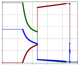
We illustrate the procedure in figure 1. A Hugoniot curve starts at initial state  $\boldsymbol {u}_0$. The shock speed reaches a maximum at $\boldsymbol {u}_1$, and the wave curve is terminated to ensure admissibility. We store the sonic speed at state $\boldsymbol {u}_1$ in the stack. The sequence of wave curves is continued by an integral curve. It terminates when $\eta (\boldsymbol {u}_2)=0$, and it is followed by a mixed curve. As the shock speed during a mixed curve is the characteristic speed during the integral curve, the speed profiles are symmetric for these two curves. When the mixed curve reaches state $\boldsymbol {u}_3$, calculated from the first point of the integral curve $\boldsymbol {u}_1$, the wave speed is equal to the sonic speed stored in the stack. Therefore, the first Hugoniot curve is continued with origin in $\boldsymbol {u}_0$ and using pressure values continuing $\boldsymbol {u}_3$.

Figure 1. Example of a configuration of wave curves. (a) A representation of the behaviour of the wave speed along the wave curves. (b) Their representation in the phase space.
3.5. Mapping wave curves to waves in the spatial domain
The Riemann problem is solved once both sequences of wave curves to the right and to the left are constructed, and the intersection point is found leading to the intermediate states.
In the spatial domain, the position of a wave  $w$ is determined by its speed $\upsilon _w$. The wave structure is created from the initial discontinuity of the Riemann problem and does not depend on time. Instead, time $t$ determines the position of the waves as
 \begin{equation} x_w=x_{init.\,discont.}+t\, \upsilon_w. \end{equation}
Hugoniot and mixed curves are associated with shock waves in the spatial domain. The shock speed is given by the last state of the wave curve, which also determines the final state of the jump discontinuity starting at the origin point. Integral curves are associated with rarefaction waves in the spatial domain, the states of one being the states of the other. These waves move with speed equal to the characteristic speed of the corresponding characteristic field.
The waves in the spatial domain are determined from the first wave curve starting at the initial state towards the wave curve that intersects with the other wave curves sequence. Due to the spatial location determined by (3.38), the sequence of waves appearing towards each direction has monotonically decreasing wave speed. If a wave curve is slower than any of the following curves, then its corresponding wave is overtaken and does not emerge in the spatial domain. The wave corresponding to the wave curve intersecting the opposite sequence always arises since there is no posterior (faster) wave.
The overtaking of waves is inherent to integral curves that break and are continued by a mixed curve (Liu Reference Liu1975). By definition, the mixed curve has the same wave speed as an integral curve but in reverse order, therefore every calculated state overtakes the origin state from the integral curve. If all the points in the integral curve are used for calculating the mixed curve, then the latest is overtaken completely, and only the jump discontinuity remains in the spatial domain. If the mixed curve is terminated (as a sonic shock or because it reaches the middle state), then the integral curve appears until the last state used for the mixed curve, and from that last point there would be a jump discontinuity, thus appearing as a composite wave in the spatial domain. Due to the overtaking, it is usual to have many more wave curves in phase space than waves in the spatial domain. However, all of them are necessarily part of the wave structure.
4. Building wave curves in non-convex SRHD with the Gaussian gamma law EoS
In this section, we derive the relations between the flow velocity and the pressure for every type of wave curve in SRHD using an EoS that induces non-convex dynamics.
We consider the phenomenological Mie–Grüneisen type of EoS (Ibáñez et al. Reference Ibáñez, Marquina, Serna and Aloy2017; Marquina, Serna & Ibáñez Reference Marquina, Serna and Ibáñez2019), known as the ‘Gaussian gamma law’ (GGL) EoS. It is defined as
 \begin{equation} P=(\gamma(\rho)-1)\rho\epsilon, \end{equation}
with
 \begin{equation} \gamma(\rho)=\gamma_0+(\gamma_1-\gamma_0)\exp({-(\rho-\rho_0)^2/\sigma_0^2}). \end{equation}
 The parameters  $\gamma _0, \gamma _1$ are such that ${1<\gamma _0<\gamma _1<2}$. The parameter $\sigma_0$ is chosen to guarantee causality and thermodynamic consistency of the EoS (Marquina et al. Reference Marquina, Serna and Ibáñez2019), and $\rho _0$ is a scale factor for the density that can be normalized. The GGL EoS is as smooth as the corresponding relativistic fundamental derivative is continuous.
The square of the relativistic sound speed for the GGL EoS is
 \begin{equation} c_s^2=\frac{\epsilon}{h}(\gamma(\rho)\,(\gamma(\rho)-1)+\rho\,\gamma'(\rho)). \end{equation}
Its fundamental derivative depends on the two first derivatives of the adiabatic index:
 \begin{equation} \mathcal{G}=\frac{1+\gamma(\rho)}{2}+\frac{\rho}{2}\, \frac{2\,\gamma(\rho)\,\gamma'(\rho)+\rho\,\gamma''(\rho)}{\gamma(\rho)\,(\gamma(\rho)-1)+\rho\,\gamma'(\rho)}. \end{equation}
Depending of the selection of the EoS parameters, the relativistic fundamental derivative (1.7) (equivalently, the nonlinearity term) reaches negative values in the domain of the EoS, therefore it exhibits thermodynamic non-convex behaviour (Ibáñez et al. Reference Ibáñez, Marquina, Serna and Aloy2017; Marquina et al. Reference Marquina, Serna and Ibáñez2019).
4.1. Hugoniot curves for GGL SRHD
We follow the procedure presented in § 3 to build the Hugoniot curves. In order to obtain values of  $\upsilon _b(P_b)$, we need to provide a way to calculate $\rho _b$ for the GGL EoS.
From (4.1) and relativistic enthalpy definition  $h=1+\epsilon +({P}/{\rho})$, we have
 \begin{equation} P=\frac{(\gamma(\rho)-1)\,\rho\,(h(\epsilon,\rho)-1)}{\gamma(\rho)}. \end{equation}
Considering the post-shock pressure  $P_b$, having a known state $a$ and using (3.14) to calculate the enthalpy, we obtain an implicit equation on $\rho _b$:
 \begin{equation} P_b=\frac{(\gamma(\rho_b)-1)\,\rho_b\,(h_b(P_b,\rho_b)-1)}{\gamma(\rho_b)}. \end{equation}
 An approximation of  $\rho _b$ can be obtained by using the Newton method. With $\rho _b$ and $P_b$, we can calculate the enthalpy $h_b$ in (3.14), and evaluate (3.11). By selecting the sign of $j$ according to the direction of the wave, we can calculate the shock speed (3.6) and flow velocity (3.10).
4.2. Integral curves for GGL SRHD
Following the procedure in § 3 to build integral curves, we particularize  $X_a^b$ in (3.30) for the GGL EoS.
Using the acoustic sound speed (4.3) in terms of the density and the internal energy, we have
 \begin{equation} X_a^b=\int_{\rho_a}^{\rho_b} \frac{c_s}{\rho}\,{{\rm d}}\rho=\int_{\rho_a}^{\rho_b} \frac{1}{\rho}\,\sqrt{\frac{\epsilon\left(\gamma(\rho)\,(\gamma(\rho)-1)+ \rho\,\gamma'(\rho)\right)}{1+\epsilon\rho}}\,{{\rm d}}\rho. \end{equation}
In order to solve this integral numerically, we need to provide an expression relating the energy and the density. We use the fact that self-similar solutions are isentropic. The first law of thermodynamics with constant entropy reads
 \begin{equation} {\rm d}\epsilon=-P\,\mathrm{d}V=\frac{P}{\rho^2}\,{\rm d}\rho. \end{equation}
For the EoS (4.1), we have
 \begin{equation} {\rm d}\epsilon=\frac{\gamma(\rho)-1}{\rho}\,{\rm d}\rho. \end{equation}
 If we consider a known state  $a$ of the integral curve that is followed by a state $b$, then we get
 \begin{equation} \epsilon_b=\epsilon_a \left(\frac{\rho_b}{\rho_a} \right)^{\gamma_0-1} \exp({(\gamma_1-\gamma_0)Y}) \end{equation}
where  $Y$ is an integral that comes from the exponential term of the adiabatic index:
 \begin{equation} Y=\int_{\rho_a}^{\rho_b} \frac{\exp\left({\dfrac{-(\rho-\rho_0)^2}{\sigma_0^2}}\right)}{\rho}\,\mathrm{d}\rho. \end{equation}
 Then, from a state  $a$ we can approximate (4.7) to a state $\rho _b$, using the value of the internal energy given by (4.10) at any intermediate point. Once this is calculated, we obtain the flow velocity using (3.30). The pressure is given by the EoS using the internal energy (4.11) and the density.
4.3. Mixed curves for GGL SRHD
For the purpose of calculating states of a mixed curve, we use the Rankine–Hugoniot conditions (3.1), where the unknown is the state after the shock. The state ahead is a point in the previous integral curve, and the shock speed is the characteristic speed in it. Using  $\Diamond$ to denote values belonging to the integral curve, we obtain the system
 $$\begin{gather} \upsilon\rho W-D^\Diamond \upsilon^\Diamond -\lambda(\rho W-D^\Diamond )=0, \end{gather}$$
 $$\begin{gather}W^2\upsilon^2\rho(1+\epsilon\gamma)+(\gamma-1)\rho\epsilon-S^\Diamond \upsilon^\Diamond -P^\Diamond -\lambda(\rho \upsilon W^2(1+\epsilon\gamma)-S^\Diamond )=0, \end{gather}$$
 $$\begin{gather}W^2\upsilon\rho(1+\epsilon\gamma)-w\upsilon\rho-S^\Diamond +D^\Diamond \upsilon^\Diamond -\lambda(\rho(1+\epsilon\gamma)W^2-(\gamma-1)\rho\epsilon-\rho W -\tau^\Diamond )=0, \end{gather}$$
where we have used  $\lambda _k(u^\Diamond )=\lambda$, $\gamma (\rho )=\gamma$ for readability. Here, $W$ is the Lorentz factor evaluated at $\upsilon$. The conserved variables here are rewritten such that the unknowns are the density, the internal energy and the velocity. Notice that $\boldsymbol {u}^\Diamond$, the integral curve state, is a trivial solution of the system.
From (4.12), we obtain a conservation equation
 \begin{equation} \rho W(\upsilon-\lambda)=D^\Diamond (\upsilon^\Diamond -\lambda) . \end{equation}
Introducing this in (4.13) and (4.14), we obtain, respectively,
 $$\begin{gather} (\gamma-1)\rho\epsilon+W(1+\gamma\epsilon)\upsilon D^\Diamond (\upsilon^\Diamond -\lambda)=S^\Diamond (\upsilon^\Diamond -\lambda)+P^\Diamond, \end{gather}$$
 $$\begin{gather}\lambda(\gamma-1)\rho\epsilon+D^\Diamond (\upsilon^\Diamond -\lambda)(W(1+\gamma\epsilon)-1)=S^\Diamond -D^\Diamond \upsilon^\Diamond -\lambda \tau^\Diamond . \end{gather}$$
 Some terms cancel out by subtracting  $\lambda$ multiplied by (4.16) from (4.17),
 \begin{equation} W(1+\gamma\epsilon)(1-\lambda \upsilon)=W^\Diamond h^\Diamond (1-\lambda v^\Diamond ), \end{equation}
and by subtracting  $\upsilon$ multiplied by (4.17) from (4.16),
 \begin{equation} \rho\epsilon(\gamma-1)(1-\lambda \upsilon)=P^\Diamond (1-\lambda \upsilon)+ D^\Diamond W^\Diamond h^\Diamond (\upsilon^\Diamond -\lambda)(\upsilon^\Diamond -\upsilon), \end{equation}
where we have simplified terms using the definition of the conserved variables. Now the system is formed by (4.15), (4.18) and (4.19).
From (4.15), we can obtain the velocity as a function of the density only:
 \begin{equation} \upsilon(\rho)=\frac{\lambda+\dfrac{D^\Diamond (\upsilon^\Diamond -\lambda)}{\rho} \sqrt{1-\lambda^2+\left(\dfrac{D^\Diamond (\upsilon^\Diamond -\lambda)}{\rho}\right)^2}}{1+ \left(\dfrac{D^\Diamond (\upsilon^\Diamond -\lambda)}{\rho}\right)^2}. \end{equation}
 The sign of the root has been selected with the criterion that  $\upsilon (\rho ^\Diamond )=\upsilon ^\Diamond$ must hold. Then the two other equations are linear in the internal energy, so we obtain
 $$\begin{gather} \epsilon=\left(\frac{W^\Diamond h^\Diamond (1-\lambda \upsilon^\Diamond )}{W(1-\lambda \upsilon)}-1\right) \frac{1}{\gamma}, \end{gather}$$
 $$\begin{gather}\epsilon=\frac{P^\Diamond (1-\lambda \upsilon)+D^\Diamond W^\Diamond h^\Diamond (\upsilon^\Diamond -\lambda)(\upsilon^\Diamond -\upsilon)}{\rho (\gamma-1)(1-\lambda \upsilon)}, \end{gather}$$
from each of them, respectively. Equating the expressions, we get an implicit equation in  $\rho$ whose zeros are density solutions of the system
 \begin{align} g(\rho) &= W(1-\lambda \upsilon)(\gamma P^\Diamond +(\gamma-1)\rho) \nonumber\\ &\quad +h^\Diamond W^\Diamond \left(\gamma W D^\Diamond (\upsilon^\Diamond -\lambda)(\upsilon^\Diamond -\upsilon)-(\gamma-1) \rho(1-\lambda \upsilon^\Diamond )\right). \end{align}
This equation can be solved using the Newton method employing as initial guess a perturbation of the density in the integral curve.
5. Example of application
In this section, we present a step by step outline for the calculation of points in each of the three types of wave curves. Then we apply the solution procedure to blast wave Riemann problems developing complex wave structure.
5.1. Practical methodology to calculate wave curves
The first wave curve developing with the origin at each initial condition is determined by the behaviour of the pressure along it and the sign of the nonlinearity factor at the initial state (see table 2).
Once the type of curve is selected, consecutive points in phase space are calculated until the end of the wave curve due to its termination conditions or to the intersection with the opposite sequence of wave curves.
Next we recap the procedure to calculate states of each type of wave curve given its origin, and present the numerical methods used to deal with the equations presented in the previous sections in the implementation of the solver.
5.1.1. Practical calculation of a Hugoniot curve
The origin state of a Hugoniot curve is the start of the jump discontinuity that would end at each calculated state of the curve, and is always the known state  $a$ in the presented formulas.
To calculate a point in a Hugoniot curve, we choose the pressure value of the new state. This pressure value has to be a continuation of the wave curves sequence in phase space. Notice that the reference value of pressure that has to be continued moves along the wave curve, but the origin state never changes. Once the pressure is selected, we calculate the corresponding density value from the EoS. For the GGL EoS, we solve (4.6) using a Newton iteration procedure. From the new density and pressure values, we can obtain the enthalpy in the new state through (3.14), the squared mass flux invariant from (3.11), and the shock speed from (3.6). In (3.11) and (3.6), we select the sign accordingly to the direction of the movement of the wave. As the initial state is always ahead, the states calculated from the initial left (right) state move to the left (right). Finally, we obtain the fluid speed at the new state using (3.10) and the shock speed (3.6).
We control the termination of a Hugoniot curve by monitoring the monotonicity of the shock speed. If it changes sign, then we perform a mesh refinement on the pressure until the termination state,  $\upsilon _s(\boldsymbol {u})'=0$, is found with a certain tolerance.
5.1.2. Practical calculation of an integral curve
To calculate a point in an integral curve, we choose the density value of the new state, a continuation of those in the wave curve sequence. This serves as the final density for the integral  $X_a^b$ in (3.29), which, depending on the EoS, may need to be solved numerically. For the GGL EoS, the integral becomes (4.7) and needs the internal energy values related to the density at any intermediate state used for numerical integration. We obtain them by solving (4.10) numerically. Finally we evaluate the fluid velocity at the new state with (3.30) and the pressure through the EoS.
Every new calculated state of an integral curve can be taken as origin for the calculation of the next state, which allows us to take small density steps that decrease the numerical error in the solution of (3.29).
An integral curve is no longer defined when the nonlinearity factor vanishes. Nevertheless, when calculating states in a discrete fashion, we never reach the exact zero where the definition equation blows up. Since the curve is defined to both sides of the zero, we can monitor the sign of the nonlinearity factor. If it changes sign, then we perform a mesh refinement on the density until the termination state,  $\eta (\boldsymbol {u})=0$, is found with a certain tolerance.
5.1.3. Practical calculation of a mixed curve
The calculation of a mixed curve depends on a preceding integral curve whose start and end states are already known. We store points of the integral curve equidistant in density to use as origin states for each point on the mixed curve. We start calculating from the last state of the integral curve, and move progressively towards its origin.
Given an origin state in the integral curve, we can solve the Rankine–Hugoniot conditions that jump to the mixed curve state. For the GGL EoS, we solve (4.23) to obtain the density of the state belonging to the mixed curve. We use a Newton method with initial guess a perturbation of the integral curve density. We verify that the convergence is not to the trivial solution but, indeed, to the closer solution as Liu (Reference Liu1975) prescribed. Then we can obtain the fluid velocity using (4.20), the internal energy by (4.21) or (4.22), and the pressure through the EoS. We have noticed that (4.23) stiffens close to the state where a mixed curve ends as a sonic shock, possibly making the root finder fail. Similar scenarios have been reported in other exact Riemann solvers (Giacomazzo & Rezzolla Reference Giacomazzo and Rezzolla2006).
If the mixed curve becomes sonic, there is no non-trivial solution to the Rankine–Hugoniot conditions beyond the integral curve state that serves as origin to the termination state of the mixed curve. In the case where we cannot find a solution, we perform mesh refinement on the integral curve to obtain a better approximation of the termination state of the mixed curve.
Mixed curves comprise the more challenging computation of the three types of wave curves. On the one hand, (4.23) needs to be solved numerically and converge specifically to one of its multiple roots, needing a criterion to select the initial guess and discriminate if the found root is appropriate. On the other hand, any refinement to the termination state, if the shock becomes sonic or if the curve is reached by the velocity in the stack, cannot be performed directly on the mixed curve. The last state needs to be found by increasing the resolution of its origin state within the integral curve.
In the following, we apply our exact Riemann solver for non-convex SRHD to two blast wave problems using the GGL EoS. We consider two sets of GGL parameters, ensuring causality and thermodynamical consistency (Marquina et al. Reference Marquina, Serna and Ibáñez2019):  $\gamma _0=4/3$, $\gamma _1=1.9$, $\rho _0=1$, $\sigma _0=1.1$ and $\gamma _0=4/3$, $\gamma _1=5/3$, $\rho _0=1$, $\sigma _0=0.6$. The spatial domain is set to $x\in [0,1]$, with initial discontinuity located at $x=0.5$. The initial conditions are gathered in table 3.
Table 3. GGL EoS parameters and Riemann problem initial conditions for the examples, taken from Marquina et al. (Reference Marquina, Serna and Ibáñez2019). The labelling of the parametrizations of the EoS is different from the reference.

The five orders of magnitude difference in the initial values of the pressure produces a strong blast wave with a thin density shell. While in convex SRHD the shell is led by a front shock, we show that in non-convex dynamics, the leading nonlinear wave can be a composite wave instead. We describe the steps of the solution procedure and present, for reference, the origin and termination state of all wave curves involved.
5.2. Blast wave 1 problem with GGL1
5.2.1. Wave curves
In a blast wave problem, the higher pressure decreases. In this case, the initial left state (larger pressure) is in a convex region ( $\mathcal {G}_{(\mathcal {R})}(\boldsymbol {u}_L)>0$) and therefore an integral curve starts to the left. The lower pressure increases and since the right initial condition is also in a convex region of the EoS ( $\mathcal {G}_{(\mathcal {R})}(\boldsymbol {u}_R)>0$), a Hugoniot curve starts to the right.
The origin and termination states of the wave curves in the sequence moving to the left are gathered in table 4. The first integral curve is terminated when the nonlinearity factor vanishes. A mixed curve follows and is calculated using points from the integral curve until it becomes a sonic shock and it is terminated. We do not indicate the origin state of the mixed curve in the table, as the origin moves along the previous integral curve. Another integral curve continues from the terminated mixed curve and does not traverse any other change of sign of the nonlinearity factor. Therefore, it is continued until its intersection with the right sequence of wave curves. The intersection in phase space takes place at  $\upsilon =0.9863$, $P=7.483$.
Table 4. Origin and termination states of the wave curves moving to the left in the blast wave 1 Riemann problem with GGL1 EoS.

The origin and termination states of the wave curves in the sequence moving to the right are gathered in table 5. The first Hugoniot curve terminates when the entropy condition fails. An integral curve follows, but encounters a zero of the nonlinearity factor and is terminated. A mixed curve therefore follows. It intersects the left sequence of wave curves before reaching the first state of the previous integral curve as origin.
Table 5. Origin and termination states of the wave curves moving to the right in the blast wave 1 Riemann problem with GGL1 EoS.

The left and right sequences of wave curves are drawn in phase space in figure 2, together with a zoom of the intersection region. The legend displays H for Hugoniot curves, I for integral curves, and M for mixed curves. We denote with L the wave curves moving left and with R the right-moving wave curves.

Figure 2. Wave curves for the exact solution of the blast wave 1 Riemann problem with GGL1 EoS. (a,b) Wave curves. (c) Zoom at the intersection region. Here, H denotes Hugoniot curve, I integral curve, and M mixed curve; L refers to left-moving wave curves, and R to right-moving wave curves.
5.2.2. Mapping of wave curves to spatial domain
Each calculated wave curve corresponds to a wave in the spatial domain. Given that their position in space depends on the wave speed, wave curves in the sequence that are slower than posterior waves are overtaken and do not appear in the solution profiles. In figure 3, we draw the evolution of the wave speed along the wave curves.

Figure 3. Wave speeds along the different wave curves for blast wave 1 problem with GGL1 EoS: (a) left-moving waves, (b) right-moving waves. (c) A zoom of the upper region of the right-moving waves.
The spatial position of a wave is calculated using (3.38). For this example  $x_{init.\,discont.}=0.5$ and we present the solution profiles at $t_f=0.4$. In the description below, we use approximations of the wave speeds for easier reading. Tables 4 and 5 contain more precise values.
The sequence to the left starts with an integral curve of increasing wave speed. It starts with  $\upsilon _w\approx -0.580$ and terminates when the wave speed is $\upsilon _w\approx 0.294$. In the spatial domain, this curve translates into a rarefaction wave extending from $x=0.268$ to $x=0.616$. The next wave curve is a mixed curve that terminates before using all the previous integral curve as origin. This translates into a shock wave in the spatial domain, a jump discontinuity to the last state of the curve, from the origin of such state. This last state has shock speed $\upsilon _w\approx -0.086$, therefore the jump is located at $x=0.464$, within the previous rarefaction wave. Indeed, the state ahead of the jump is the rarefaction state origin of the last state in the mixed curve. The last part of the rarefaction is therefore overtaken. Finally, another integral curve follows from this position until the intermediate state. This is reached with $\upsilon _w \approx 0.864$, so the last rarefaction to the left ends at $x=0.844$. Nevertheless, the contact discontinuity moves with speed equal to the fluid speed at the intermediate state, which is $\upsilon \approx 0.986$. The difference of velocity makes a constant state appear between the last rarefaction to the left and the contact discontinuity.
The sequence to the right starts with a Hugoniot curve that terminates at the fastest wave speed of the whole sequence. It translates into a shock wave, a jump discontinuity from its origin, the initial right state, to the last state of the curve with speed  $\upsilon _w\approx 0.996$, therefore at position $x=0.898$. An integral curve follows, extending from the shock. But this integral curve is followed by a mixed curve, so as in the left sequence case, not all the corresponding rarefaction states appear in the spatial domain. It shows up until the state that serves as origin to the mixed curve point that intersects the left sequence. This happens when the integral curve has wave speed $\upsilon _w\approx 0.991$, therefore at $x=0.896$. At this point, there is the shock wave corresponding to the mixed curve, jumping from the rarefaction to the intermediate state. Since this speed is faster than the fluid at the equilibrium, there is also a constant state between the last wave to the right and the contact discontinuity.
The profiles for density, pressure and velocity are shown in figure 4, along a detail of the density shell. We represent with points the key states calculated for jumps discontinuities, and the rarefactions to better show their curvature. We add lines connecting the dots to better see the jumps of shock waves and the constant states. The three waves described to the left are clearly seen in all profiles, while in order to appreciate the details of the composite wave to the right, we need to focus on the density shell. It features the two shocks united by a rarefaction fan as the front structure of the blast wave.

Figure 4. (a) Density, (b) zoom of its density shell, (c) pressure and (d) velocity profiles for the blast wave 1 problem with GGL1 EoS.
5.3. Blast wave 2 problem with GGL2
5.3.1. Wave curves
In this blast wave problem, the initial left state (larger pressure) is in a region of negative nonlinearity term ( $\mathcal {G}_{(\mathcal {R})}(\boldsymbol {u}_L)<0$) and therefore a Hugoniot curve starts to the left. The lower pressure increases, and since the right initial condition is in a convex region of the EoS ( $\mathcal {G}_{(\mathcal {R})}(\boldsymbol {u}_R)>0$), a Hugoniot curve starts to the right.
The origin and termination states of the wave curves in the sequence moving to the left are gathered in table 6. The first Hugoniot curve terminates when the entropy condition fails. It is continued in phase space by an integral curve that intersects the right sequence of wave curves. The intersection in phase space takes place at  $\upsilon =0.9794$, $P=4.922$.
Table 6. Origin and termination states of the wave curves moving to the left in the blast wave 2 Riemann problem with GGL2 EoS.

The origin and termination states of the wave curves in the sequence moving to the right are gathered in table 7. The first Hugoniot curve terminates when the entropy condition fails. An integral curve follows. When it reaches a zero of the nonlinearity factor, it is terminated. A mixed curve therefore follows, and it is calculated until it uses the start of the previous integral curve as origin. The first Hugoniot curve resumes with origin in the initial state and continues the sequence. It intersects the left sequence of wave curves.
Table 7. Origin and termination states of the wave curves moving to the right in the blast wave 2 Riemann problem with GGL2 EoS.

The left and right sequences of wave curves are drawn in phase space in figure 5, together with a zoom of the intersection region. The legend displays H for Hugoniot curves, I for integral curves, and M for mixed curves. We denote with L the left-moving wave curves, and with R the right-moving wave curves.

Figure 5. Wave curves for the exact solution of the blast wave 2 Riemann problem with GGL2 EoS. (a,b) Wave curves. (c) Zoom at the intersection region. Here, H denotes Hugoniot curve, I integral curve, and M mixed curve; L refers to left-moving wave curves, and R to right-moving wave curves.
5.3.2. Mapping of wave curves to spatial domain
The position of the waves in the spatial domain can be deduced from the wave speeds at the termination state of each wave curve. As in the previous example, we present the solution profiles at final time  $t_f=0.4$.
The sequence to the left starts with a Hugoniot curve that terminates with shock speed  $\upsilon _w\approx -0.839$ and therefore translates in the spatial domain to a shock wave at $x=0.164$. The following integral curve represents a rarefaction wave. The head moves with the same speed as the shock, and the tail reaches the middle equilibrium state with $\upsilon _w\approx 0.920$, therefore ending the rarefaction at $x=0.868$. The contact discontinuity moves with the speed of the fluid, which at the equilibrium state is $\upsilon \approx 0.974$, therefore there is a constant state between the tail of the rarefaction and the contact discontinuity, located at $x=0.890$.
The sequence of wave curves to the right comprises four wave curves. Nevertheless, it is the shock wave corresponding to the last calculated Hugoniot curve that is faster, with shock speed  $\upsilon _w\approx 0.989$. Therefore, this shock wave overtakes the waves from the previous wave curves, and unites the initial condition with the equilibrium state at position $x=0.896$. There is a constant state from this shock until the contact discontinuity.
The profiles for density, pressure and velocity are shown in figure 6. The wave moving to the left is the composite wave described from the left wave curve sequence. To the right, as the front of the density shell, we observe a single shock wave although there are four wave curves in the right sequence.

Figure 6. (a) Density, (b) zoom of its density shell, (c) pressure and (d) velocity profiles for the blast wave 2 problem with GGL2 EoS.
To illustrate the complexity of non-convex dynamics, we introduce small perturbations in the density of the blast wave 2 Riemann problem. The perturbations can lead to quite different wave structures in the spatial domain, although the sequence of wave curves in phase space is similar. We gather the initial conditions in table 8.
Table 8. Perturbations proposed for the blast wave 2 Riemann problem.
The different density values at the right initial condition modify the states of the right wave curves sequence, which in turn change the intersection with the left sequence in phase space. We draw the intersection of the wave curves in phase space in figure 7. In perturbation 1, the intersection takes place along the integral curve of the right sequence of wave curves. In perturbation 2, it happens in the mixed curve that follows the integral curve when it is terminated.

Figure 7. Wave curves of perturbations 1 and 2 from the blast wave 2 problem with GGL2 EoS.
The density shells obtained from the data with perturbations are depicted in figure 8. The front of the shell is a composite wave in both cases. In perturbation 1, we observe a shock and a rarefaction wave, since there is a Hugoniot curve followed by an integral curve in phase space. In perturbation 2, we observe a composite wave of two shocks with a rarefaction fan in the middle, analogous to the one observed in the blast wave 1 problem. Since the intersection of the wave curves happen shortly after the beginning of the mixed curve, this one does not overtake the rarefaction completely.

Figure 8. Density shells of perturbations 1 and 2 from the blast wave 2 problem.
6. Conclusions
We have proposed a procedure to calculate the general analytical solution of the Riemann problem in SRHD when the system is closed with a non-convex EoS. We present the equations defining the different wave curves in the pressure–velocity phase space: Hugoniot curves, integral curves and mixed curves, as well as their termination and continuation conditions. We describe the procedure to construct the exact solution and relate the wave curves to waves in the spatial domain. We apply the exact Riemann solver to relativistic blast wave problems that showcase the complex wave dynamics arising in non-convex SRHD.
Funding
This work was partially supported by Spanish Government grant PID2020-118236GB-I00.
Declaration of interests
The authors report no conflict of interest.


 Open access