


1. Introduction
The nature and structure of small-scale vortex structures have received considerable attention in turbulence research and are typically defined as concentrated regions of high enstrophy with life-times greater than the characteristic time scale of the flow (Dubief & Delcayre Reference Dubief and Delcayre2000). These vortex tubes, filaments or so-called worms are the most prominent small-scale structures at the dissipation scale having been identified in early numerical simulations and experimentally observed by, amongst others, Siggia (Reference Siggia1981), Kerr (Reference Kerr1985), She, Jackson & Orszag (Reference She, Jackson and Orszag1990), Vincent & Meneguzzi (Reference Vincent and Meneguzzi1991), Cadot, Douady & Couder (Reference Cadot, Douady and Couder1995), Jiménez et al. (Reference Jiménez, Wray, Saffman and Rogallo1993), Jiménez & Wray (Reference Jiménez and Wray1998) and Ishihara, Gotoh & Kaneda (Reference Ishihara, Gotoh and Kaneda2009). Over the last few decades, the growth in computational power and new experimental methods have enabled observation of small-scale vortices at ever higher Reynolds numbers and in an increasingly wide range of flows. They appear to have some universal features such as the preferential alignment of the vorticity vector with the direction of intermediate principal strain found by Ashurst et al. (Reference Ashurst, Kerstein, Kerr and Gibson1987) and their average radius of about  $5\eta$, where $\eta$ is the Kolmogorov length scale, as verified in homogeneous isotropic turbulence (Jiménez et al. Reference Jiménez, Wray, Saffman and Rogallo1993; Jiménez & Wray Reference Jiménez and Wray1998; Ghira, Elsinga & Da Silva Reference Ghira, Elsinga and Da Silva2022), jets (Ganapathisubramani, Lakshminarasimhan & Clemens Reference Ganapathisubramani, Lakshminarasimhan and Clemens2008; da Silva, dos Reis & Pereira Reference da Silva, dos Reis and Pereira2011), channel flows (Kang, Tanahashi & Miyauchi Reference Kang, Tanahashi and Miyauchi2009) and stratified flows (Neamtu-Halic et al. Reference Neamtu-Halic, Mollicone, van Reeuwijk and Holzner2021). Although the alignment of the vorticity vector with the intermediate principal strain holds at small scales, and has been observed in a wide range of flows, at larger length scales the vorticity preferentially aligns instead with the most stretching principal strain (Ishihara, Yamazaki & Kaneda Reference Ishihara, Yamazaki and Kaneda2001; Leung, Swaminathan & Davidson Reference Leung, Swaminathan and Davidson2012).
In the seminal direct numerical simulation (DNS) of homogeneous isotropic turbulence by Jiménez et al. (Reference Jiménez, Wray, Saffman and Rogallo1993), it was found that small-scale vortex tubes produced low levels of stretching demonstrating that self-amplification did not play a significant role in their evolution. Jiménez et al. (Reference Jiménez, Wray, Saffman and Rogallo1993) draw attention to the resemblance between these small-scale vortices and axially stretched stable Burgers vortices by considering their stability and lack of coupling with the strain field. The implication of this is significant as it showed that at the small scale, these high-enstrophy vortex structures do not play a significant role in the overall dynamics of the flow and can therefore be considered passive. This was also emphasized by Tsinober (Reference Tsinober2009), who noted that the lack of self-amplification via interaction with the strain field means that the worms are rather passive and decoupled from the strain field. This is in direct contrast with sheet-like, strained vortices whose presence modifies the local strain field significantly (Moffatt, Kida & Ohkitani Reference Moffatt, Kida and Ohkitani1994; Le Dizes, Rossi & Moffatt Reference Le Dizes, Rossi and Moffatt1996; Davidson Reference Davidson2015). In a later study, Jiménez & Wray (Reference Jiménez and Wray1998) investigated the relationship between stretching at the points of maximum vorticity inside the worms with their corresponding radii. The joint probability density function (p.d.f.) of these two parameters showed good agreement with the values of radii based on the stable Burgers vortex model. These observations have been expanded to include other flows, for example the turbulent plane jet by da Silva et al. (Reference da Silva, dos Reis and Pereira2011). However, the lack of interaction with the strain field does not mean that vortex tubes do not interact with the local flow in other important ways, for example through the exchange of mass and momentum with their surroundings. These interactions have not been investigated in detail to date. In this paper we employ a fully resolved experimental data set and DNS to investigate the interaction of vortex filaments with the surrounding flow. This is done by implementing a robust method to detect the boundary of the vortices and then analysing conditional flow features to show that they entrain and detrain mass and momentum.
When it comes to precisely defining and detecting small-scale vortical structures, researchers usually adopt one of two well-known and broadly used approaches: thresholding on the vorticity (Hussain Reference Hussain1986; Jiménez et al. Reference Jiménez, Wray, Saffman and Rogallo1993; da Silva et al. Reference da Silva, dos Reis and Pereira2011; Ghira et al. Reference Ghira, Elsinga and Da Silva2022) or the vorticity relative to the strain field (Hua & Klein Reference Hua and Klein1998). The problem with these classical detection methods is that they are arbitrary and depend on the observer's frame of reference (Haller Reference Haller2005). For instance, using classical detection methods, an observer in fixed laboratory coordinates will not identify the same vortex structures as an observer that is moving with the flow. Methods developed in a recent string of research articles, summarized in the review paper by Haller (Reference Haller2015), have been shown to overcome these limitations and permit identification of objective (i.e. observer-independent) coherent structures necessary for repeatable experiments. The method proposed by Haller et al. (Reference Haller, Hadjighasem, Farazmand and Huhn2016) to detect rotationally coherent structures from the vorticity field was previously adapted and implemented to identify large-scale vortex structures in three-dimensional turbulence measurements of a gravity flow by Neamtu-Halic et al. (Reference Neamtu-Halic, Krug, Haller and Holzner2019). The primary advantage of this method is that it provides an objectively defined vortex boundary permitting an investigation of the conditional fluxes across it to reveal how small-scale vortical structures interact with the surrounding flow from both a local and global perspective.
The aim of this study is to investigate the interaction of objectively identified small-scale vortical structures in more detail than what has been done so far in the literature to obtain a better understanding of their interaction with the surrounding flow. We adopt an approach which treats them as turbulent structures embedded in a turbulent background flow and borrows a similar methodological approach to that used to investigate local entrainment across turbulent–non-turbulent interfaces (TNTIs) as exemplified by Mathew & Basu (Reference Mathew and Basu2002), Westerweel et al. (Reference Westerweel, Fukushima, Pedersen and Hunt2005), Holzner & Lüthi (Reference Holzner and Lüthi2011), Wolf et al. (Reference Wolf, Lüthi, Holzner, Krug, Kinzelbach and Tsinober2012), Mistry et al. (Reference Mistry, Philip, Dawson and Marusic2016) and Mistry, Philip & Dawson (Reference Mistry, Philip and Dawson2019) in order to evaluate their interaction with the surrounding flow by evaluating the enstrophy transport equation which enables direct comparison with the Burgers vortex model. (Although we adopt a similar methodology to that of these studies, we are not suggesting an equivalence between the boundary of a vortex structure and the TNTI.) To do this we make use of two data sets. The first is a fully resolved three-dimensional experimental data set of stationary homogeneous turbulence measured at the centre of a von Kármán mixing flow with a Reynolds number based on the Taylor microscale of  $R_\lambda =179$ (Lawson & Dawson Reference Lawson and Dawson2014, Reference Lawson and Dawson2015). Until recently, experimental access to the full velocity gradient tensor of small-scale turbulence at reasonably high Reynolds number has remained elusive and almost all previous studies of small-scale vortical structures have been restricted to DNS data sets without an experimental counterpart. This is the first time that the three-dimensional objective vortex definition of Haller et al. (Reference Haller, Hadjighasem, Farazmand and Huhn2016) has been implemented on an experimental data set of resolved small-scale turbulence. To complement the experimental data set, results are compared with the DNS data set of homogeneous isotropic turbulence of Li et al. (Reference Li, Perlman, Wan, Yang, Meneveau, Burns, Chen, Szalay and Eyink2008) at $R_\lambda =418$.
The paper is organized as follows. Section 2 describes the large-scale von Kármán facility, a brief description of the experimental data set from Lawson & Dawson (Reference Lawson and Dawson2014, Reference Lawson and Dawson2015) and the implementation of the detection method by Haller et al. (Reference Haller, Hadjighasem, Farazmand and Huhn2016) for objective Eulerian coherent structures (OECS) as well as how to calculate the entrainment velocity from the enstrophy transport equation derived by Holzner & Lüthi (Reference Holzner and Lüthi2011). The results in § 3 begin with presenting volume-averaged and conditional statistics of the small-scale vortices to illustrate consistency between the experimental and DNS data sets. Attention is then turned to statistics of entrainment and the balance of the different terms in the enstrophy transport equation. The enstrophy balance is considered from two different perspectives, the first being conditioning on the radial direction of the vortices and the second from conditioning on their axes. The results are discussed and interpreted in the context of expected quantities from the Burgers vortex model.
2. Methods
2.1. Description of facility and data sets
The experimental data set used in this study is from the scanning particle image velocimetry measurements of homogeneous axisymmetric turbulence produced by the large von Kármán mixing flow facility reported in Lawson & Dawson (Reference Lawson and Dawson2014, Reference Lawson and Dawson2015). Due to the large size of the facility and the slow rotation rate of the impellers, spatially and temporally resolved measurements at the Kolmogorov scale were achievable. A two-dimensional schematic of the experimental facility is shown in figure 1 highlighting key dimensions and the general flow pattern. The flow inside the tank can be considered a superposition of a stationary axisymmetric shear flow generated by the counter-rotating impellers and a centrifugal pumping leading to a radially inward flow along the mid-plane of the tank and axial flow away from the geometric centre along the rotational symmetry axis. The shear generated by the counter-rotation of the impellers results in a region of homogeneous, axisymmetric turbulence near the centre of the tank with a near-zero mean velocity in all directions (Lawson & Dawson Reference Lawson and Dawson2014, Reference Lawson and Dawson2015).

Figure 1. Two-dimensional schematic of the large tank facility with dimensions. The blue lines show the flow pattern in azimuthal (horizontal) planes and the black lines show the flow pattern in an axial (vertical) plane passing the geometric centre of the tank. The measurement volume is represented by a square at the centre of the tank.
The facility is comprised of a large dodecagonal Perspex tank that is  $2\,{\rm m}$ tall and $2\,{\rm m}$ in cross-section that was filled with water. The impellers at the top and bottom of the tank were $1.6\,{\rm m}$ in diameter and operated at constant angular velocity in a counter-rotating mode. Vertical baffles were placed at each vertex with the same height as the tank protruding $100\,{\rm mm}$ into the flow. The Reynolds number based on the impeller radius defined as $Re =\varOmega _I R_I^2 /\nu$, where $\varOmega _I$ is the rate of rotation of the impellers, $R_I$ is the radius of the impellers and $\nu$ is the kinematic viscosity of the flow, was 23 000. The Reynolds number based on Taylor microscale was $R_\lambda =179$ and the Kolmogorov length scale was $\eta =0.926\,{\rm mm}$. The measurement volume was located at the geometric centre of the tank with dimensions $L_x \times L_y \times L_z =129\,{\rm mm} \times 128\,{\rm mm} \times 26.2\,{\rm mm}$. The spatial resolution of the data set was approximately $1\eta$ over a non-dimensional measurement volume of $L_x/\eta \times L_y/\eta \times L_z/\eta =135 \times 134 \times 25.4$. The data set consists of 1003 statistically independent volumes constructed from a time series of 10 volumetric vector fields with a particle image velocimetry separation time of $\approx 0.068\tau _{\eta }$, where $\tau _{\eta }$ is the Kolmogorov time scale. There was no spatial averaging applied to the data. A predictor-corrector scheme was implemented in a Lagrangian tracking algorithm performing forward and backward in time over the time-resolved velocity fields to minimize noise (Novara & Scarano Reference Novara and Scarano2013). The data set is of very low noise and highly resolved enabling direct comparisons with DNS up to third-order gradient statistics (Lawson & Dawson Reference Lawson and Dawson2014, Reference Lawson and Dawson2015).
A DNS data set of forced isotropic turbulence of  $R_{\lambda }=418$ from the Johns Hopkins Turbulence Database (Li et al. Reference Li, Perlman, Wan, Yang, Meneveau, Burns, Chen, Szalay and Eyink2008) was also analysed for comparison with the experimental data set. This DNS data set is a time series of a periodic forced cube with $1024^3$ nodes over five large-eddy turnover times. Fifty independent volumes of the flow (snapshots of the cubes with $128^3$ nodes) with a dimension size of $L_x/\eta \times L_y/\eta \times L_z/\eta =279 \times 279 \times 279$ were chosen at random time steps over the five large-eddy turnover times. The spatial resolution is about $2.2\eta$.
2.2. Detection of OECS
To analyse the intense small-scale vortex structures a robust detection method based on the definition of OECS proposed by Haller et al. (Reference Haller, Hadjighasem, Farazmand and Huhn2016) was implemented. The OECS are detected using a scalar field corresponding to the instantaneous vorticity deviation (IVD) which is defined in (2.1):
 \begin{equation} {\rm IVD}(\boldsymbol{x},t)=|\boldsymbol{\omega}(\boldsymbol{x},t)-\bar{\boldsymbol{\omega}}(t)|, \end{equation}
where  $\boldsymbol {\omega }(\boldsymbol {x},t)$ is the vorticity vector at the time step $t$ at point $\boldsymbol {x}$ in space and $\bar {\boldsymbol {\omega }}(t)$ is the average value of vorticity over the volume of the flow at the time step $t$. Since the DNS is homogeneous and isotropic and the experimental data are also approximately homogeneous and isotropic with negligible mean flow, the normalization by the volumetric average is not sensitive to volume size. However, in other flows that are not homogeneous and isotropic, the normalization by the volumetric average in the OECS method may introduce a dependence of the results on volume size that should be taken into account. This definition is an observer-independent (objective) scalar field that represents the local rotation rate of fluid elements. The OECS are defined as a nested family of tubular level surfaces of ${\rm IVD}(\boldsymbol {x},t)$ in which the value of ${\rm IVD}(\boldsymbol {x},t)$ is non-increasing when moving outward from the centre. Along each of these tubular surfaces the rotation rates of the fluid elements are equal. The boundary is defined as the outermost almost convex level surface of ${\rm IVD}(\boldsymbol {x},t)$ and the centre is the maximum level surface of the nested family. As discussed in Haller et al. (Reference Haller, Hadjighasem, Farazmand and Huhn2016), this definition detects vortical structures that are observer-independent and ensures instantaneous coherence in the rate of their material bulk rotation. No thresholding is therefore needed to define/detect these vortical structures. We refer the reader to Haller (Reference Haller2015) and Haller et al. (Reference Haller, Hadjighasem, Farazmand and Huhn2016) for further details.
The numerical detection algorithm used to detect the three-dimensional OECS to the data set of Lawson & Dawson (Reference Lawson and Dawson2015) is described in detail by Neamtu-Halic et al. (Reference Neamtu-Halic, Krug, Haller and Holzner2019). Therefore we only provide a brief description of the detection algorithm for completeness. The detection algorithm consists of three main steps. In the first step, the vorticity field is evaluated followed by the IVD scalar field according to (2.1). In the second step, ridges corresponding to the local maximum values of the IVD are detected using a three-dimensional gradient ascent method starting from point clouds of high spatial gradient of IVD values as the initial guess. The Cauchy–Lipschitz theorem was used to solve the ordinary differential equation of the gradient ascent algorithm. The ridges represent the centre lines of the vortex structures. In the third step, two-dimensional contours of IVD are calculated on planes locally normal to the ridges which are then used to build three-dimensional level surfaces for the structures. The outermost convex level surface is chosen as the boundary of the structure. Successful implementation for the detection of small-scale structures requires a fully resolved three-dimensional three-component velocity field with low levels of noise. So far, this has only been applied to the experimental data set by Neamtu-Halic et al. (Reference Neamtu-Halic, Krug, Haller and Holzner2019) where the resulting structures were comparatively large on average ( $R\approx 15\eta$).
2.3. Equations and models
To investigate the flow field within and immediately surrounding the vortex filaments as well as compare with the Burgers vortex model, the detected boundaries of the vortex filaments are treated with the methodological approach applied to the TNTI enabling the investigation of the fluxes passing across it. To do this we evaluate various terms in the enstrophy transport equation (2.2), where the first term on the right-hand side ( $2 \omega _i \omega _j s_{ij}$) corresponds to the inviscid production/destruction of enstrophy by vortex stretching/compression, the second term ( $\nu ({\partial ^2\omega ^2}/{\partial x_j \partial x_j})$) is the viscous diffusion of enstrophy due to the presence of gradients and the final term ( $-2\nu ({\partial \omega _i}/{\partial x_j})({\partial \omega _i}/{\partial x_j})$) corresponds to the viscous dissipation of enstrophy (Pope Reference Pope2000; Tsinober Reference Tsinober2009):
 \begin{equation} \frac{{\rm D}\omega^2}{{\rm D}t}=2 \omega_i \omega_j s_{ij}+\nu\frac{\partial^2\omega^2}{\partial x_j \partial x_j}-2\nu\frac{\partial \omega_i}{\partial x_j}\frac{\partial \omega_i}{\partial x_j}. \end{equation}
 Using the enstrophy transport equation, Holzner & Lüthi (Reference Holzner and Lüthi2011) derived an equation for the entrainment velocity,  $v_n$, which can be applied at the boundary of the structures:
 \begin{equation} v_n={-}\dfrac{2 \omega_i \omega_j s_{ij}}{|\boldsymbol{\nabla}\boldsymbol{\omega^2}|}-\dfrac{\nu\dfrac{\partial^2\omega^2}{\partial x_j \partial x_j}}{|\boldsymbol{\nabla}\boldsymbol{\omega^2}|}+\dfrac{2\nu\dfrac{\partial \omega_i}{\partial x_j}\dfrac{\partial \omega_i}{\partial x_j}}{|\boldsymbol{\nabla}\boldsymbol{\omega^2}|}, \end{equation}
where the entrainment velocity,  $v_n$, is defined as $\boldsymbol {V}=v_n \skew 2\hat {\boldsymbol {n}}=\boldsymbol {u^s}-\boldsymbol {u}$. In this definition, $\boldsymbol {u^s}$ is the velocity vector of an iso-surface element, for example the boundary of the vortex structure, $\boldsymbol {u}$ is the fluid velocity vector at the iso-surface and $\skew 2\hat {\boldsymbol {n}}={\boldsymbol {\nabla }\boldsymbol {\omega ^2}}/{|\boldsymbol {\nabla }\boldsymbol {\omega ^2}|}$ is the iso-surface normal vector. Based on this definition, $v_n\leq 0$ corresponds to the entrainment of fluid from the surroundings into the structures whereas $v_n>0$ corresponds to the detrainment of fluid from inside the structures to the surrounding fluid (Holzner & Lüthi Reference Holzner and Lüthi2011; Mistry et al. Reference Mistry, Philip and Dawson2019). Based on the entrainment velocity, the local flux of other quantities across the boundary can be calculated through multiplication with $v_n$. For example, the specific flux of enstrophy defined as $v_n\omega ^2$ and the kinetic energy $v_n u_iu_i$. Equation (2.3) is valid on an iso-surface of enstrophy and follows from the fact that for an observer moving with an iso-surface (denoted by the superscript s) the iso-level is constant, i.e. $D^s\omega ^2/D^st=0$ (Holzner & Lüthi Reference Holzner and Lüthi2011). According to the definition of the IVD in (2.1) and given that $\bar {\boldsymbol{\omega} }(t)$ is a constant under statistically stationary and homogeneous conditions, it follows that $D^s\omega ^2/D^st=0$ and $D^s({\rm IVD})/D^st=0$ are interchangeable. Thus, (2.3) can be used to calculate the entrainment velocity at the boundary of detected vortex structures where the IVD is considered.
We also compare features of the small-scale vortical structures with the classical Burgers vortex model to further elucidate similarities and differences. For a Burgers vortex (Burgers Reference Burgers1948), it is assumed that the flow is incompressible and the vorticity field is unidirectional. The vorticity field is normally assumed to be one-dimensional or both the vorticity field and the strain field axisymmetric (Saffman Reference Saffman1995). A sketch of Burgers vortex is shown in figure 2. The stability of the Burgers vortex results from a balance between the inviscid effects of vortex stretching and viscous effects of vorticity diffusion and dissipation. This leads to outflow along the axis of symmetry ( $u_z$) and radial entrainment ( $u_r$) to maintain the rotational energy and mass conservation. The radial velocity is shown in (2.4) where $\alpha >0$ is the strain of the flow and it is a constant. Equation (2.5) governs the enstrophy profile where $R_B$ is the Burgers vortex radius and $\nu$ is the kinematic viscosity. In the Burgers vortex model all the terms in the enstrophy transport equation (2.2) can be evaluated analytically by using (2.5)–(2.9) (Taveira & da Silva Reference Taveira and da Silva2014; Davidson Reference Davidson2015; Watanabe et al. Reference Watanabe, Jaulino, Taveira, da Silva, Nagata and Sakai2017).
 \begin{gather} u_r(r)={-}\tfrac{1}{2}\alpha r, \end{gather}
 \begin{gather} \omega_z(r)=\omega_0 \exp{\left(-\frac{r^2}{R_B^2}\right)}; \omega_0=\omega(r=0), R_B^2=\frac{4\nu}{\alpha}, \end{gather}
 \begin{gather} 2\omega_i\omega_js_{ij}=2\omega_z^2(r) \alpha =2\omega_0^2\alpha\exp{\left({-}2\frac{r^2}{R_B^2}\right)}, \end{gather}
 \begin{gather} \nu\frac{\partial^2\omega^2}{\partial x_j \partial x_j}=\nu\frac{1}{r}\frac{\partial}{\partial r}\left(r\frac{\partial\omega_z^2(r)}{\partial r}\right)=2\alpha\omega_0^2\left(2\frac{r^2}{R_B^2}-1\right)\exp{\left({-}2\frac{r^2}{R_B^2}\right)}, \end{gather}
 \begin{gather} -2\nu\frac{\partial \omega_i}{\partial x_j}\frac{\partial \omega_i}{\partial x_j}={-}2\nu\left(\frac{\partial \omega_z(r)}{\partial r}\right)^2={-}2\alpha\omega_0^2\left(\frac{r^2}{R_{B}^2}\right)\exp{\left({-}2\frac{r^2}{R_B^2}\right)}, \end{gather}
 \begin{gather} \frac{{\rm D}\omega^2}{{\rm D}t}=u_r(r)\frac{\partial\omega_z^2(r)}{\partial r}=2\alpha\omega_0^2\left(\frac{r^2}{R_{B}^2}\right)\exp{\left({-}2\frac{r^2}{R_B^2}\right)}. \end{gather}
Figure 2. The Burgers vortex model.
3. Results
3.1. Statistics of the structures and the flow field
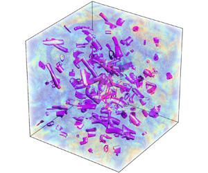
In this section, volume-averaged statistics and statistics conditioned on the inside of the structures from both the experimental and DNS data sets are presented and discussed. An example of the objectively identified three-dimensional intense vortical structures in a measured volume of the flow is shown in figure 3(a). The black curved lines denote the centre of the structures, the magenta surfaces the boundary of each structure and the colour shading corresponds to the normalized enstrophy field,  ${\omega ^2}/{\langle \omega ^2\rangle _s}$, where $\langle \,\sim\, \rangle _s$ is the volume average of the corresponding snapshot. In total, 12 466 structures were detected over the 1003 snapshots of the experimental data set. A similar example is shown in figure 3(b) obtained from a single volume of the DNS data set. Overall 9274 structures were detected over the 50 snapshots of the DNS data set.

Figure 3. Examples of the structures (magenta surfaces) in single volumes of the (a) experimental and (b) DNS data sets with the corresponding enstrophy values. The enstrophy values are normalized by the corresponding volume average of the snapshots,  $\langle \omega ^2\rangle _s$. The spatial dimensions are normalized by the Kolmogorov length scale, $\eta$.
Figure 4 shows the p.d.f.s of the normalized radius of the structures for the experiment and DNS defined as  $R^*={R}/{\eta }$, where $R$ is the distance between the centre of the structure and its boundary. As the cross-sections of the structures are contorted, the radii are evaluated at various random points along the boundary of each structure with the average radius of the structures found to be $\langle R\rangle =5.1\eta$ which is in a good agreement with previous studies (Jiménez et al. Reference Jiménez, Wray, Saffman and Rogallo1993; Ganapathisubramani et al. Reference Ganapathisubramani, Lakshminarasimhan and Clemens2008; da Silva et al. Reference da Silva, dos Reis and Pereira2011; Neamtu-Halic et al. Reference Neamtu-Halic, Mollicone, van Reeuwijk and Holzner2021). The volume of the structures occupied $1.4\,\%$ of the whole volume of the flow field which is also in a good agreement with the value of ${\approx }1\,\%$ reported by Jiménez et al. (Reference Jiménez, Wray, Saffman and Rogallo1993). This confirms that both the identification method and the experimental data set are sufficiently well resolved and consistent with DNS as expected from previous work of Lawson & Dawson (Reference Lawson and Dawson2015).

Figure 4. The p.d.f.s of normalized radius of the structures ( ${R}/{\eta }$) of the (a) experimental and (b) DNS data sets.
The objective detection method used herein initially follows similar steps to the thresholding method used in Jiménez et al. (Reference Jiménez, Wray, Saffman and Rogallo1993). However, the methods diverge once the process of determining the centre lines of the vortex structures takes place. In Jiménez et al. (Reference Jiménez, Wray, Saffman and Rogallo1993) the enstrophy profile of the vortex is assumed to decay exponentially to detect the boundary, whereas the objective detection method detects the outermost almost convex iso-surface as the boundary. Thus, one might expect small variations in the radii of the detected vortex structures to occur depending on the method. However, figure 4, i.e.  $\mathrm {p.d.f.}(R/\eta )$, is similar to the analogous figures in the works of Jiménez et al. (Reference Jiménez, Wray, Saffman and Rogallo1993), Jiménez & Wray (Reference Jiménez and Wray1998), da Silva et al. (Reference da Silva, dos Reis and Pereira2011) and Ghira et al. (Reference Ghira, Elsinga and Da Silva2022) where the thresholding detection method is used giving confidence that the two methods yield similar results for resolved homogeneous and isotropic data sets.
To quantify the rotational energy and intermittency of the small-scale structures, p.d.f.s of normalized enstrophy  ${\omega ^2}/{\langle \omega ^2\rangle }$ are plotted in figure 5(a) for the experiment (black lines) and DNS (grey lines), where $\langle \omega ^2\rangle$ is the enstrophy spatially averaged over the whole measurement volume and all the snapshots. The dashed lines show the p.d.f.s throughout the volume, whereas the solid lines show the p.d.f.s conditioned on the inside of the structures. A logarithmic binning is used to calculate the p.d.f.s and are plotted on $\log \unicode{x2013}\log$ scale. Good agreement is found across the data sets. The p.d.f.s from the experiment and DNS both intersect at around ${\omega ^2}/{\langle \omega ^2\rangle }=1$. When ${\omega ^2}/{\langle \omega ^2\rangle }<1$, the p.d.f.s of the volumetric enstrophy are significantly higher and peak at ${\omega ^2}/{\langle \omega ^2\rangle }\approx 10^{-2}$ and also extend to much lower values ${\omega ^2}/{\langle \omega ^2\rangle }\approx 10^{-6}$ than the p.d.f.s conditioned on the inside of the structures. When ${\omega ^2}/{\langle \omega ^2\rangle }>1$, conditioned on the structures shows slightly greater enstrophy values before falling off with similar values to the volumetric average. The p.d.f.s show that increasingly high-enstrophy events are similarly rare in the volume-averaged and conditional statistics, whereas low-enstrophy events are much less prevalent for the conditioned statistics.

Figure 5. The p.d.f.s of normalized (a) enstrophy and (b) dissipation of the structures (solid lines) and volume (dashed lines). The black curves represent the experiment and the grey curves represent DNS.
We can draw a similar comparison between the local and volumetric dissipation where it is normalized as  ${\epsilon }/{\langle \epsilon \rangle }$. The dissipation, $\epsilon$, is defined as $\epsilon =2\nu s_{ij} s_{ij}$, where $\nu$ is the kinematic viscosity of the flow and $s_{ij}=({\partial u_i}/{\partial x_j}+{\partial u_j}/{\partial x_i})/2$ is the rate of strain tensor. The ensemble average dissipation is denoted as $\langle \epsilon \rangle$ and evaluated over the full data set. Figure 5(b) shows the p.d.f.s of the normalized dissipation for the whole volume (dashed lines) and conditioned on the inside of the structures (solid lines) for both the experiments and DNS. Again it is observed that the volumetric and conditioned p.d.f.s intersect when ${\epsilon }/{\langle \epsilon \rangle }=1$. When ${\epsilon }/{\langle \epsilon \rangle }>1$ the p.d.f.s show that the structures contribute slightly higher dissipation compared with the volume. On the other hand, the structures contribute less than the total volume when ${\epsilon }/{\langle \epsilon \rangle }<1$. Nevertheless, the small-scale vortices still produce significant dissipation. Similar to the p.d.f.s of enstrophy, the probability that the vortex structures contain higher dissipation events is greater when compared to the whole volume. However, the difference for dissipation is not as large as for the case of enstrophy. This means that the structures are an intense realization of enstrophy with some overlap with regions of high dissipation/strain in the flow field (Davidson Reference Davidson2015).
To better understand the relationship between enstrophy and dissipation, spatial correlations in the from of joint p.d.f.s (j.p.d.f.s) are plotted in figure 6. These show that the volumetric j.p.d.f.s (dashed contours) for the experimental and DNS data sets exhibit a similar distribution to that reported in Yeung, Donzis & Sreenivasan (Reference Yeung, Donzis and Sreenivasan2012). When conditioned on the inside of the small-scale structures, shown by the solid contours, the j.p.d.f.s are shifted upwards and to the right towards higher values of enstrophy and dissipation. The j.p.d.f.s also show a preferred diagonal alignment (more symmetric with respect to the diagonal) which is consistent with an increase in local  $R_{\lambda }$ as discussed in the work of Yeung et al. (Reference Yeung, Donzis and Sreenivasan2012). This means that there is a preferential increase in the joint probability of extreme events of enstrophy and dissipation inside the structures. Furthermore, enstrophy and dissipation appear to scale similarly inside the structures which suggests a physical dependence between vorticity and strain even though it is not clear which one of them is the cause and which one is the effect (Jiménez et al. Reference Jiménez, Wray, Saffman and Rogallo1993).

Figure 6. Joint p.d.f.s of normalized enstrophy and dissipation for the (a) experiment and (b) DNS. The solid contours represent the structures and the dashed contours represent the volume.
The importance of the relationship between vorticity and the rate of strain dates back to Taylor (Reference Taylor1938) who postulated that the stretching of small-scale vortices caused them to break up into yet smaller vortices and was therefore expected to be an important mechanism in the turbulent cascade. However, it was not until the DNS work by Ashurst et al. (Reference Ashurst, Kerstein, Kerr and Gibson1987) which permitted access to the full velocity gradient tensor which showed that instantaneously, the vorticity vector is aligned with the intermediate eigenvector of the rate of strain tensor, rather than the extensive eigenvector, and is predominantly positive. The alignment of the vectors is observer-independent and is important to the phenomenon of vortex stretching ( $2\omega _i\omega _js_{ij}$) which produces enstrophy (Tsinober Reference Tsinober2009).
The alignment between the vorticity vector  $\boldsymbol {\omega }=(\omega _1,\omega _2,\omega _3)$ and the eigenvectors of the rate of strain tensor $\boldsymbol {e}=(\boldsymbol{e}_1,\boldsymbol{e}_2,\boldsymbol{e}_3)$, where ordering of the eigenvalues is $\sigma _1\geq \sigma _2\geq \sigma _3$, can be investigated by plotting the cosine of the angles between these vectors: $\cos \theta _i=\boldsymbol{e}_i\boldsymbol {\cdot }{\boldsymbol {\omega }}/{|\boldsymbol {\omega }|}$. From the continuity equation, it follows that the sum $\sigma _1+\sigma _2+\sigma _3=0$ which means that $\sigma _1$ is always positive and its corresponding eigenvector, $\boldsymbol{e}_1$, is the extensive eigenvector. In contrast, $\sigma _3$ is always negative and its corresponding eigenvector, $\boldsymbol{e}_3$, is compressive. The value of $\sigma _2$ is determined by the sum of $\sigma _1$ and $\sigma _3$ and can be either negative or positive and is the intermediate eigenvalue with a corresponding eigenvector, $\boldsymbol{e}_2$.
The p.d.f.s of the cosine of the angles between the vorticity vector and the eigenvectors are plotted in figure 7(a,b) where the solid and dashed lines correspond to the alignments conditioned on the inside of the structures and the volume, respectively. Overall, the experimental data and DNS show excellent agreement. Considering the volume-based statistics first, the vorticity vector and the intermediate eigenvector are well aligned with each other as the peak values of the p.d.f.s occur at  $\cos \theta _2=\pm 1$ and appears to be a universal aspect of turbulent flow (Elsinga & Marusic Reference Elsinga and Marusic2010). The alignment between the vorticity vector and the compressive eigenvector shows a peak at $\cos \theta _3=0$ showing that the two vectors are predominantly normal to each other, whereas the extensive eigenvector indicates no preferential alignment. When conditioned on the structures, the vorticity vector is also aligned with the intermediate eigenvector but it is normal to both the extensive and compressive eigenvectors. A much higher peak at $\cos \theta _3=0$ is observed when conditioned on the inside of the structures. These results indicate that vorticity vectors inside the structures exhibit a strong preferred alignment with the intermediate eigenvector but normal to the extensive and compressive eigenvectors (Frisch Reference Frisch1995; Tsinober Reference Tsinober2009; Buaria, Bodenschatz & Pumir Reference Buaria, Bodenschatz and Pumir2020). Since the vorticity vector is only aligned with the intermediate eigenvector, we consider the distribution of the eigenvalues and, in particular, $\sigma _2$. Figure 8(a,b) plots p.d.f.s of eigenvalues of the rate of strain tensor for the same cases as considered in figure 7. As expected, $\sigma _1>0$ and $\sigma _3<0$ for the volume and structures whereas the p.d.f. of $\sigma _2$ contains both negative and positive values but is positive on average, $\langle \sigma _2\rangle >0$. An insight into enstrophy production is gained by considering the average vortex stretching which can be written as $\langle 2\omega _i\omega _js_{ij}\rangle =2\omega ^2(\langle \sigma _1\cos ^2\theta _1\rangle +\langle \sigma _2\cos ^2\theta _2\rangle +\langle \sigma _3\cos ^2\theta _3\rangle )$ (Tsinober Reference Tsinober2009). This relation is used to calculate the shares, relative to each alignment, in the total production/destruction of enstrophy, i.e. ${\langle \sigma _j\cos ^2\theta _j\rangle }/{\sqrt {\sum \langle \sigma _i\cos ^2\theta _i\rangle ^2}}$. This is shown in table 1. Clearly the contributions of the extensive and compressive eigenvalues become weaker in favour of the intermediate eigenvalue inside the structures as expected from figure 7. However, the contribution from the extensive eigenvalue remains prominent and, overall, the ratio of enstrophy production to destruction increases. This is consistent with the picture that, on average, the production of enstrophy via vortex stretching inside the structures is more significant compared with the flow field as a whole.

Figure 7. Alignment between vorticity vector and the eigenvectors of the rate of strain tensor for the (a) experiment and (b) DNS. The solid lines represent the structures and the dashed lines represent the volume.

Figure 8. The p.d.f.s of the normalized eigenvalues of the rate of strain tensor for the (a) experiment and (b) DNS. The solid lines represent the structures and the dashed lines represent the volume.
Table 1. Enstrophy production (vortex stretching) contribution shares due to alignment between the vorticity vector and the rate of strain eigenvectors and the corresponding eigenvalues for the experiment and DNS.

3.2. Kinematics/dynamics of the structures
3.2.1. Entrainment
To further elucidate the local flow field in a frame of reference relative to the high-enstrophy small-scale structures, we consider them as being embedded in a predominantly quiescent flow and their detected boundaries are treated with the methodological approach applied at the TNTI. We then calculate the entrainment/detrainment velocity and the rate of enstrophy production, diffusion and dissipation across the boundaries using (2.3) and (2.2). Analysing the interaction of structures in this way will reveal how they interact with the flow in terms of mass and momentum exchange and permit direct comparison with the Burgers vortex model.
Figure 9 shows the p.d.f.s of the entrainment velocity,  $v_n$, vortex stretching, enstrophy diffusion and dissipation terms from (2.3) for the experiment (solid lines) and DNS (dashed lines). The values are normalized by the corresponding Kolmogorov velocity scale, $u_{\eta }=(\nu \langle \epsilon \rangle )^{1/4}$. With the exception of enstrophy dissipation, the peaks in the p.d.f. of the various terms are all slightly negative and exhibit non-Gaussian distributions. Overall good agreement between the DNS and the experiments is observed. The p.d.f. of the entrainment velocity $v_n$ is similar to those observed in other flows at the TNTI (Holzner & Lüthi Reference Holzner and Lüthi2011; Wolf et al. Reference Wolf, Lüthi, Holzner, Krug, Kinzelbach and Tsinober2012; Mistry et al. Reference Mistry, Philip and Dawson2019) which shows a fine balance in favour of entrainment over detrainment noting that the tail on the left-hand side, which corresponds to entrainment, has higher values compared with the right-hand side which corresponds to detrainment. This demonstrates that, on average, the structures are radially entraining fluid from the quiescent surroundings as $\langle v_n \rangle <0$. The contribution of vortex stretching to the entrainment velocity, $-2 \omega _i \omega _j s_{ij}/|\boldsymbol {\nabla }\boldsymbol {\omega ^2}|$, is shown by the red line and exhibits higher probabilities than the entrainment velocity which is balanced by the contribution of viscous diffusion of enstrophy. Viscous diffusion peaks slightly on the negative side but shows higher probabilities in the tails when $v_n/u_{\eta }>0$. On the right-hand side, the tails of the viscous effects of enstrophy dissipation and diffusion have higher p.d.f. values compared with vortex stretching. This provides direct evidence that vortex stretching is a dominant mechanism that drives entrainment ( $v_n<0$) whereas the viscous effects of enstrophy diffusion and dissipation contribute predominantly to detrainment ( $v_n>0$). This is in contrast with the behaviour of viscous and inviscid budgets across the TNTI of free shear flow where the viscous effect is always dominant in both entrainment and detrainment regions and is an indication of viscous/laminar superlayer at the turbulence boundary (Holzner & Lüthi Reference Holzner and Lüthi2011). However, the behaviour of the vortex boundary is similar to that of the turbulent–turbulent interface where vortex stretching is dominant and viscous superlayer is not present (Kankanwadi & Buxton Reference Kankanwadi and Buxton2022).

Figure 9. The p.d.f.s of normalized entrainment velocity,  $v_n/u_\eta$, at the boundary of the structures and its components (budgets: vortex stretching, $-2 \omega _i \omega _j s_{ij}/(|\boldsymbol {\nabla }\boldsymbol {\omega ^2}|u_\eta )$; diffusion, $-\nu ({\partial ^2\omega ^2}/{\partial x_j \partial x_j})/(|\boldsymbol {\nabla }\boldsymbol {\omega ^2}|u_\eta )$; dissipation, $2\nu ({\partial \omega _i}/{\partial x_j})({\partial \omega _i}/{\partial x_j})/(|\boldsymbol {\nabla }\boldsymbol {\omega ^2}|u_\eta )$) for the experiment (solid lines) and DNS (dashed lines).
The picture that emerges is that the overall behaviour of the small-scale structures appears similar to that of stable Burgers vortices where the radial entrainment of surrounding low-enstrophy fluid into the vortex is the result of a competition between vortex stretching, enstrophy diffusion and enstrophy dissipation. In a stable Burgers vortex the radial entrainment velocity is  $u_r=-({\alpha }/{2})r$, where $\alpha$ is a positive constant (the strain rate) and hence $u_r<0$ (Davidson Reference Davidson2015) and is consistent with the average picture of the detected vortex structures observed in the experimental and DNS data sets even though the local statistics are not in full agreement with the Burgers vortex model.
We examine the local dependence of the entrainment velocity on the radius (size) of the structures by plotting the j.p.d.f.s of the normalized entrainment velocity,  $v_n/u_\eta$, and the normalized radius, $R/\eta$, in figure 10. The experimental data are presented with solid lines and DNS with dashed lines as previously. The drop-shaped j.p.d.f.s are very slightly skewed towards the region of negative entrainment velocity which means that over all the sizes of $R/\eta$ plotted, the structures are on average radially entraining fluid from their surroundings. The peak of the correlation between the magnitude of entrainment velocity and radius occurs when $2\lesssim R/\eta \lesssim 6$. This shows that the entrainment/detrainment of the structures is most active when the local radius is between approximately $2\eta$ and $6\eta$.

Figure 10. Joint p.d.f.s of normalized entrainment velocity,  $v_n/u_\eta$, and normalized radius of the structures, $R/\eta$, for the experiment (solid contours) and DNS (dashed contours).
Next, we investigate how entrainment varies both radially and along the axial direction of the structures. In figure 11(a), we plot the average entrainment velocity conditioned on the radial and axial directions of the vortices,  $({v_n}/{u_{\eta }})({r}/{R},{l}/{\eta })$. Since the detected vortex structures are nested families of IVD iso-surfaces, the iso surfaces of IVD correspond to iso-surfaces of enstrophy as discussed in § 2.3. Thus, the entrainment velocity and the budgets in (2.3) can be calculated anywhere inside and in the vicinity of structures. The result can be interpreted as the radial velocity relative to the local iso-enstrophy surface when away from the boundary of the vortex, or alternatively, the entrainment velocity that holds for varying choice of enstrophy iso-surface boundaries. Since the length of the vortices is cropped by the finite size of the observation volume in the experiment, we here focus on DNS data only. The maximum entrainment velocity is on average located in the central region of the vortices extending $\approx \pm 5\eta$ along the vortex axis ( $r/R=0$) and radially outwards to about half the radius. Moving along the axis of the vortex along $r/R=0$ the $v_n/u_{\eta }$ decays towards both ends of the vortices to near zero values. Since the vortices occupy a finite volume of the domain, statistical stationarity would require that on average there is no gain or loss of mass for the average structure. Given the net radial entrainment observed here, one would expect a net detrainment across the boundary at the tips of the structure. The axial decrease of $v_n$ is consistent with that argument even though we do not observe a change of sign over the considered length, presumably because our detection method crops the structure before the tip which is a singular point where the cross sectional area approaches zero.

Figure 11. Filled contours of average normalized entrainment velocity and its budgets (terms in (2.3)) in radial ( ${r}/{R}$) and axial ( ${l}/{\eta }$) directions of the structures for the DNS data set: (a) entrainment velocity, (b) vortex stretching, (c) diffusion and (d) dissipation.
To investigate the spatial pattern of the different contributions to entrainment, we consider the terms (budgets) on the right-hand side of (2.3) conditioned on the radial and axial directions plotted in figure 11(b–d) for the DNS data set. Contour of vortex stretching shows a strong contribution in favour of entrainment with maximum negative values concentrated along the vortex axis decaying to very low levels near the vortex boundary. The data show a slight peak centred at  $l/\eta =0$ extending $\approx \pm 5 l/\eta$ before decaying along the vortex length. The effects of enstrophy diffusion, shown in figure 11(c), exhibit similar behaviour but in favour of detrainment. Figure 11(d) shows comparatively low, but slightly positive uniform values of enstrophy dissipation inside the vortices in favour of detrainment. Greater values of dissipation are found outside the vortices. The contribution of dissipation to the overall balance of the entrainment/detrainment velocity is small.
The Burgers vortex is a one-dimensional model and cannot capture any heterogeneity along the vortex axis by definition. However, it can still be a good model for the radial dynamics. To investigate the similarities and differences of the vortex filaments with Burgers vortices in more detail, we now compare statistical quantities from the experimental and DNS data with the quantities predicted by the Burgers vortex model (Jiménez et al. Reference Jiménez, Wray, Saffman and Rogallo1993; Jiménez & Wray Reference Jiménez and Wray1998; da Silva et al. Reference da Silva, dos Reis and Pereira2011; Watanabe et al. Reference Watanabe, Jaulino, Taveira, da Silva, Nagata and Sakai2017; Ghira et al. Reference Ghira, Elsinga and Da Silva2022). Beginning with the radii of the filaments, p.d.f.s of the ratio of measured radius of the structures from the experiments and DNS to the equivalent Burgers radius,  $R/R_B$, are plotted in figure 12. Here $R_B$ was calculated for the structures based on the stretching values along the centre lines, $\alpha _0=\omega _i\omega _js_{ij}/\omega _0^2$ at $r=0$, using the formula $R_B=\sqrt {4\nu /\alpha _{0}}$ in (2.5). The overall trends of the p.d.f.s from the experiment and DNS are in reasonably good agreement. The main differences are that the experimental data are more skewed on the left-hand side of ${R}/{R_B}=1$ with a slightly different slope for vortices with larger radii. The maximum probabilities occur between ${R}/{R_B}\approx 0.65$ and $0.75$ for both the experiments and DNS as well as small differences in the mean $\langle {R}/{R_B}\rangle =0.95$ and $1.1$. These data show that, on average, the radius of the structures and the equivalent Burgers vortex radius obtained from the experimental data are in good agreement with numerical studies, such as the DNS of Jiménez & Wray (Reference Jiménez and Wray1998) and da Silva et al. (Reference da Silva, dos Reis and Pereira2011), but there are some variations in the local statistics. In the DNS studies of Jiménez et al. (Reference Jiménez, Wray, Saffman and Rogallo1993), Jiménez & Wray (Reference Jiménez and Wray1998), da Silva et al. (Reference da Silva, dos Reis and Pereira2011) and Ghira et al. (Reference Ghira, Elsinga and Da Silva2022), the peak value of $\mathrm {p.d.f.}(R/R_B)$ occurs at $R/R_B=1$, slightly different from figure 12 in the present study. We believe this slight difference is due to the vortex detection method being used. In the above-mentioned studies, a thresholding detection method based on exponential decay of enstrophy in the radial direction (following the Burgers vortex model) was used. Here, no assumption is made about the form of the enstrophy decay.

Figure 12. The p.d.f.s of the ratio between radius of the structures and the equivalent Burgers vortex radius for the experiment (solid line) and DNS (dashed line).
Another feature of the Burgers vortex model is that the radial enstrophy distribution in the vortex follows an exponential profile from the centre line. To test the robustness of this assumption, enstrophy profiles as well as profiles of the mean deviation of the structures for the experimental and the DNS data sets are plotted for comparison. The mean radial profiles of the normalized enstrophy of the vortices and the equivalent Burgers vortex model are plotted in figure 13(a) for the experiments and DNS with black lines as well as the model values for the equivalent Burgers vortices in grey line. Good agreement between the model, experiments and DNS is found near the vortex core,  ${r}/{R}=0$. Moving away from the vortex core, both the experiments and DNS depart from the Burgers model which predicts a faster decay with $r$. Although the trends for the experiments and DNS are similar, it is difficult to untangle whether the Burgers model overestimates the decay of enstrophy towards the boundary of the structures or whether the resolution of the experiments and DNS underestimates the decay in enstrophy. Figure 13(b) plots the deviation of the experiments and DNS from the Burgers model by calculating
 \begin{equation} \delta\left(\frac{r}{R}\right)=\left\langle\frac{\omega^2\left(\dfrac{r}{R}\right) -\omega^2_B\left(\dfrac{r}{R_B}\right)}{\omega_0^2}\right\rangle \times 100\, (\%) \end{equation}
for the experimental and DNS data sets within the range of  $0\leq {r}/{R}\leq 2$. The curves show the mean radial profile of $\delta$. As can be seen from this figure, the local agreement is poor away from the vortex core in both cases which is postulated to be at least partly related to a lack of spatial resolution.

Figure 13. Enstrophy profiles. (a) The mean radial profile of the normalized enstrophy of the vortices and the equivalent Burgers vortex model for the experiments and DNS and (b) the deviation of the experiments and DNS from the Burgers model.
We next compare the ratio of the measured entrainment velocity with the entrainment velocity predicted from the Burgers vortex model. The equivalent entrainment velocity is calculated using the radial velocity formula at the boundary,  $v_{n,B}=u_{r=R_B}=-({\alpha _{0}}/{2})R_B$ (Davidson Reference Davidson2015). Figure 14 plots the p.d.f.s of the entrainment velocity ratio for the experiment (solid line) and DNS (dashed line). For the experiment, the peak of the p.d.f. occurs at $v_n/v_{n,B}\approx 0.8$ and the mean value is $\langle v_n/v_{n,B}\rangle =0.79$, whereas for DNS the peak is at $v_n/v_{n,B}\approx 0.9$ and the mean value is $\langle v_n/v_{n,B} \rangle =1.1$. Overall, the fact that $\langle v_n/v_{n,B} \rangle \approx 1$ shows that the Burgers model reasonably captures the entrainment velocity. Similar to the case of the p.d.f.s of radii (figure 12), the distributions are non-Gaussian with the positive tails having larger values away from $v_n/v_{n,B}=1$.

Figure 14. The p.d.f.s of the ratio between the entrainment velocity of the structures and the equivalent entrainment velocity from the Burgers vortex model for the experiment (solid line) and DNS (dashed line).
3.2.2. Enstrophy balance
The different terms (budgets) of the enstrophy transport equation (2.2) are now investigated along the radial and axial directions of the structures in a similar manner to that in § 3.2.1. To construct a picture of how enstrophy is distributed in a vortex, figure 15 plots filled contours of the average enstrophy profile conditioned on the radial and axial directions for the DNS data only and not the experiment as the length of the vortices is cropped by the finite size of the observation volume in the experiment. On average, the peak of enstrophy occurs at the centre of the vortex, i.e.  $({r}/{R},{l}/{\eta })=(0,0)$, which decays in the radial direction towards the vortex boundary and along the vortex axis but to a lesser extent.

Figure 15. Filled contours of average normalized enstrophy ( ${\omega ^2}/{\langle \omega ^2\rangle }$) in radial ( ${r}/{R}$) and axial ( ${l}/{\eta }$) directions of the structures for the DNS data set.
The normalized conditional averaged radial profiles of the different terms in the enstrophy transport equation are shown in figure 16 for the experiments (solid lines), DNS (dashed lines) and the equivalent Burgers vortices (with dot markers). All cases considered show reasonably similar trends indicative of having similar governing physics. On average, at the centre of the structures, the viscous terms of diffusion with a near-negligible contribution from dissipation are balanced by inviscid vortex stretching as exhibited by the material derivative of enstrophy tending close to zero. Marching towards the boundary from the vortex core, the absolute values of both vortex stretching and diffusion decrease whilst the dissipation increases. The rate of decrease is greater for the diffusion term. Together this results in the total derivative of enstrophy increasing to a peak at  ${r}/{R}\approx 0.7$ followed by a gentle decay towards zero. In the region ${r}/{R_B}>1$ of the Burgers vortex model, the viscous diffusion term dominates over the inviscid vortex stretching term. This behaviour is qualitatively similar to that of viscous superlayer at TNTI. However, in contrast with the Burgers vortex model and TNTI, the inviscid vortex stretching term is still dominant over the viscous diffusion term in the ${r}/{R_B}>1$ region of the detected vortex structures. Comparing the radial distribution of diffusion and dissipation shows that in the regions near the core, diffusion is the major contribution to the viscous effects, whereas near the vortex boundary dissipation becomes the dominant contributor.

Figure 16. Normalized enstrophy transport equation terms (material derivative of enstrophy  $({{\rm D}\omega ^2}/{{\rm D}t})\times \langle \omega ^2\rangle ^{-3/2}$, vortex stretching $2 \omega _i \omega _j s_{ij}\times \langle \omega ^2\rangle ^{-3/2}$, enstrophy diffusion $\nu ({\partial ^2\omega ^2}/{\partial x_j \partial x_j})\times \langle \omega ^2\rangle ^{-3/2}$ and enstrophy dissipation $-2\nu ({\partial \omega _i}/{\partial x_j})({\partial \omega _i}/{\partial x_j})\times \langle \omega ^2\rangle ^{-3/2}$) conditioned on the radial direction of the structures for the cases of the experiment (solid lines), equivalent Burgers vortex of the experiment (solid lines with dot markers), DNS (dashed lines) and equivalent Burgers vortex of the DNS (dashed lines with dot markers).
Similar to § 3.2.1, plotting the enstrophy transport equation terms (2.2) conditionally averaged on the radial and axial directions of the structures can provide a more complete picture of the active physical phenomena inside the structures. Here we only consider the vortices from the DNS data set and not the equivalent Burgers vortices. The reason is that the Burgers vortex model by definition is infinitely long and the quantities of interest, i.e. enstrophy and the terms in the enstrophy transport equation (equations (2.5)–(2.9)), are independent of the axial distance. Figure 17 plots the terms (budgets) of the enstrophy transport equation (2.2). In the radial direction, figure 17 confirms figure 16, and in the axial direction they show the decay of all the quantities considered which is in contrast with the Burgers vortex model.

Figure 17. Filled contours of average normalized enstrophy transport budgets (terms in (2.2)) in radial ( ${r}/{R}$) and axial ( ${l}/{\eta }$) directions of the structures for the DNS data set: (a) material derivative of enstrophy, (b) vortex stretching, (c) diffusion and (d) dissipation.
4. Conclusion
In this paper we investigated how small-scale vortex structures interact locally with the surrounding quiescent flow using a temporally and spatially resolved experimental data set of homogeneous turbulence of a von Kármán mixing flow and a DNS data set of forced isotropic turbulence. To detect the boundary of the small-scale vortex structures about which the local entrainment can be evaluated, an objective definition to identify the vortical structures introduced by Haller et al. (Reference Haller, Hadjighasem, Farazmand and Huhn2016) was implemented on both data sets and was the first successful implementation in experimentally resolved measurements of small-scale turbulence at high Reynolds number. The average radius of the vortex structures was found to be  $5.1\eta$ and that they occupied about $1.4\,\%$ of the measured flow volume on average in agreement with the reported values in the literature ( $\approx 5\eta$ and $\approx 1\,\%$). Comparing p.d.f.s of volume-averaged enstrophy and dissipation with those conditioned on the inside of the structures revealed that the latter contained higher peak values of enstrophy and dissipation but a decreased probability of low-enstrophy and low-dissipation events. These differences between the volume- and structure-averaged p.d.f.s were more pronounced for enstrophy and the enstrophy production to destruction ratio was found to be significantly higher inside the vortex structures. Volume-averaged and structure-averaged j.p.d.f.s of enstrophy and dissipation were found to scale similarly inside the vortex structures. The alignments between the vorticity vector and the rate of strain eigenvectors showed that inside the vortex structures the vorticity vectors were aligned with the intermediate eigenvector and normal to the compressive and extensional eigenvectors.
By considering the vortex structures as being embedded in a predominantly quiescent flow and conditioning on their boundary, the entrainment velocity and enstrophy budgets were determined. The p.d.f. of entrainment velocity exhibits a non-Gaussian distribution of entrainment and detrainment skewed slightly in favour of entrainment. The p.d.f. and the fine balance in favour of entrainment over detrainment is remarkably similar to the p.d.f.s of entrainment velocity observed across the TNTI reported in boundary layers and jets. The entrainment velocity was found to reach a peak near the vortex core decaying radially outwards towards the vortex boundary and along its axis. The decrease in the magnitude of the entrainment velocity was consistent with the flow being statistically stationary (the vortices cannot grow on average) and the net radial entrainment is expected to be balanced by the net detrainment at the ends of the vortices. A strong correlation between entrainment and vortex stretching was observed (inviscid effect) whereas detrainment was found to be correlated with enstrophy diffusion and dissipation events (viscous effects). This is in contrast with what is observed at the TNTI in free shear flow where the viscous effect is dominant due to the presence of the viscous/laminar superlayer. However, the behaviour of vortex boundary is similar to that of turbulent–turbulent interface where vortex stretching (inviscid effect) is dominant and viscous superlayer is no longer present. The j.p.d.f. of radius and entrainment velocity showed that entrainment/detrainment was most active when the local radii of the vortices were between  $2\eta$ and $6\eta$. A direct comparison with Burgers vortices was performed with both the experimental and the DNS data sets. The p.d.f.s of the local radius were non-Gaussian but good agreement between the experimental data, DNS and the equivalent Burgers vortex was found. Compared with the DNS and experimental data, the Burgers vortex model overestimates the rate of decay in the enstrophy profile of the vortices. Conditional budgets of the enstrophy transport equation were examined and compared with the Burgers model confirming that the competition between vortex stretching and diffusion was the dominant mechanism. It was found that marching towards the boundary both vortex stretching and diffusion gradually weakened as dissipation strengthened with all terms approaching zero just outside the vortex boundary.
Declaration of interests
The authors report no conflict of interest.


 Open access