


1. Introduction
Dense suspensions composed of mixtures of particles and fluid are ubiquitous in natural phenomena and industrial processes (Larson Reference Larson1999; Wagner & Brady Reference Wagner and Brady2009). For a sufficiently large volume fraction of particles,  $\varPhi$, the suspensions can exhibit a wide range of nonlinear phenomena, including yielding, shear thinning or thickening, and shear jamming (Guazzelli & Morris Reference Guazzelli and Morris2011; Morris Reference Morris2020; Nabizadeh, Singh & Jamali Reference Nabizadeh, Singh and Jamali2022), which has stimulated decades of research in the rheology and physics community (Wagner & Brady Reference Wagner and Brady2009; Guazzelli & Pouliquen Reference Guazzelli and Pouliquen2018). In particular, discontinuous shear thickening (DST), where the suspension viscosity, $\eta$, increases over several orders of magnitude, has recently been understood as a transition from lubricated to frictional particle interactions when the applied stress overcomes the interparticle repulsion (Fernandez et al. Reference Fernandez, Mani, Rinaldi, Kadau, Mosquet, Lombois-Burger, Cayer-Barrioz, Herrmann, Spencer and Isa2013; Seto et al. Reference Seto, Mari, Morris and Denn2013; Brown & Jaeger Reference Brown and Jaeger2014; Wyart & Cates Reference Wyart and Cates2014). Readers may refer to Morris (Reference Morris2020) for a recent review. The constitutive curve of such a suspension, relating the shear stress $\tau$ and the shear rate $\dot {\gamma }$, displays an $\mathsf{\textit{S}}$-shape in which a negatively sloped region connects the lubricated branch of low-viscosity at low stresses and the frictional branch of high-viscosity at high stresses (Brown & Jaeger Reference Brown and Jaeger2014; Mari et al. Reference Mari, Seto, Morris and Denn2015; Pan et al. Reference Pan, de Cagny, Weber and Bonn2015). Because of the characteristic $\mathrm {d} \dot {\gamma } / \mathrm {d} \tau \leqslant 0$, the steady uniform state of a suspension under shear may become unstable and reduced to large spatiotemporal fluctuations of stress and densities (Lootens, Van Damme & Hébraud Reference Lootens, Van Damme and Hébraud2003; Rathee, Blair & Urbach Reference Rathee, Blair and Urbach2017, Reference Rathee, Blair and Urbach2020). Structures and patterns, such as gradient banding (Hu, Boltenhagen & Pine Reference Hu, Boltenhagen and Pine1998; Olmsted Reference Olmsted2008) and vorticity banding (Chacko et al. Reference Chacko, Mari, Cates and Fielding2018; Saint-Michel, Gibaud & Manneville Reference Saint-Michel, Gibaud and Manneville2018), may appear as a consequence. Those inhomogeneities, either transient or periodic (Hermes et al. Reference Hermes, Guy, Poon, Poy, Cates and Wyart2016; Ovarlez et al. Reference Ovarlez, Vu Nguyen Le, Smit, Fall, Mari, Chatté and Colin2020), challenge the mean-field description of a shear-thickening suspension. Nevertheless, little is known about the disturbance growth in shear thickening suspensions in flow configurations beyond simple shear (Darbois Texier et al. Reference Darbois Texier, Lhuissier, Forterre and Metzger2020; Rathee, Blair & Urbach Reference Rathee, Blair and Urbach2021). Moreover, although boundary confinements are proposed as essential for the shear-thickening of non-Brownian suspensions (Brown & Jaeger Reference Brown and Jaeger2014), their influence on the instability development in such systems, if any, have yet to be explored.
This paper investigates the instability arising in the flow direction in dense non-Brownian suspensions under orbital shaking. A novel unsteady dynamics where density waves self-organize into a hexagonal pattern is observed, accompanied by large spatial stress fluctuations. Our result shows that it is closely related to the shear thickening of the suspension. Moreover, the essential role of boundary conditions in the development of heterogeneity is discussed.
2. Experimental protocol
The suspension consists of deionized water mixed with cornstarch particles of an average size  $d=15 \ {\mathrm {\mu }}{\rm m}$, confined within an open cylindrical container. The mass density of dry starch particles, $\rho _p$, is $1.61\ {\rm kg}\ {\rm m}^{-3}$. When preparing density-matched suspensions, caesium chloride is added to the solution. The container is subjected to a horizontal orbital vibration, i.e. a circular translational motion of the entire platform. The oscillation frequency, $f$, can be tuned from $0.5$ to $8.33\ {\rm Hz}$ with a fixed amplitude $A = 5\ {\rm mm}$ indicating the radius of the orbital motion (figure 1a). An acrylic plate can be optionally laid on the surface of the suspension, either moving with the container or fixed in the laboratory reference. The following experiments are performed in the free surface configuration, unless stated otherwise. A monochrome light emitting diode panel from below illuminates the suspension. A high-speed camera (Microtron EoSens 1.1cxp2) is fixed in the laboratory frame of reference, recording the light transmission. The spatial resolution is 0.23 mm pixel $^{-1}$. The local thickness of suspension, $h$, can be measured on demand via an in-house-built laser profilometry (Zhao, de Jong & van der Meer Reference Zhao, de Jong and van der Meer2015), and the typical resolution of $h$ is $61~{\mathrm {\mu }}{\rm m}~{\rm pixel}^{-1}$ in the current configuration. The transmission of the bottom light is through scattering events. We established a one-dimensional multiscattering model, and the ratio between the incoming flux and the transmitted flux is given as $F(\phi,h) = 1 + a \phi ^bh$. The parameters $a$ and $b$ are calibrated with the light intensity attenuation data for uniform cornstarch suspensions. Readers may find the calibration data and method justification in Appendix A. By simultaneously measuring $h$ and $F(\phi,h)$, the local volume fraction, $\phi$, can be calculated. An example is given in figure 1g–h, where both $h$ and $\phi$ are measured. The container has a diameter of $32 \ {\rm cm}$ and a height of $5 {\rm cm}$. Though the sidewall is critical for the surface wave of a Newtonian fluid of low viscosity, such as water, under orbital shaking (Reclari et al. Reference Reclari, Dreyer, Tissot, Obreschkow, Wurm and Farhat2014), its effect is ignored here, as changing the diameter of the container from 32 cm to 16 cm does not alter the phenomena studied in this work. The system is then defined by three major experimental parameters: the oscillation frequency $f$; the global particle packing fraction $\varPhi$; the average thickness of the suspension $h_0$. We first report our main observations in a reference system of $\varPhi = 0.42$ and $h_0 = 5\ {\rm mm}$. The influence of $\varPhi$ and the top confinement will be discussed afterwards.

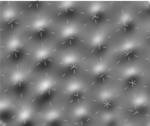
Figure 1. (a) A schematic of the experimental set-up. The light transmission is captured by a charge-coupled device (CCD) positioned at the top. (b) A top-view snapshot of the suspension at  $f = 7.67 \ {\rm Hz}$ (supplementary movie 1 available at https://doi.org/10.1017/jfm.2024.234). The dark (bright) areas correspond to the high (low) $\phi$ regions. (c–f) A zoomed-in area at different phases in one oscillation period. The dashed circle denotes the trajectory of the centre of the dense area. An example of local particle fraction, $\phi$, measurement is shown in (g). The arrow indicates the instantaneous flow direction. Note that $\phi$ is computed accounting for both the light transmission ratio and the surface deformation. Panel (h) illustrates the surface height along the dashed line in (g).
3. Results
3.1. Experimental results
The suspension is uniform at low oscillation frequencies. However, when  $f$ is increased beyond $3.67\ {\rm Hz}$, high-density regions appear suddenly, followed by low-density tails. These density patches self-organize into a hexagonal pattern with a further increase of $f$, as shown in figure 1(b). Individual dense regions move in a circular path at the same frequency $f$ precisely, with little changes in location and size over time (figure 1c–f; refer to supplementary materials for multimedia view). The motion of the dense regions is defined by the position of the highest density locally. The typical diameter of the circular path, denoted as $d_w$, measures 13.3 mm, which is larger than the orbit of the container. In such a state, the surface becomes uneven too, introducing a peak-to-valley height difference $\Delta h\approx 1\ {\rm mm}$. Dense/loose regions correspond to peaks/valleys (figure 1g). As the suspension is bounded by the air–liquid interface, the observation indicates a non-uniform normal stress distribution accompanying the density inhomogeneity, a hallmark of non-Newtonian behaviour.
As reported by Oyarte Gálvez et al. (Reference Oyarte Gálvez, de Beer, van der Meer and Pons2017), the interaction force profile shows a hysteresis when corn starch particles are pressed into contact. However, the inhomogeneity transition here is reversible, which implies that the dense regions in our experiments are not permanent aggregates of contacting particles. To reveal the microscopic nature of the observed inhomogeneity, we measure the velocity of tracer particles near the suspension surface,  $u_p$, and local packing fraction, $\phi$, simultaneously at a point on the path of a high-density region. Both $u_p$ and $\phi$ vary in phase with the same period as the oscillation, as shown in figure 2, i.e. particles in denser regions tend to move faster. However, the particle velocity remains lower than that of the density pattern, indicating that the motion of the observed density pattern is the propagation of density waves. Furthermore, the gradient of $\phi$ in the wavefront is significantly steeper than that at the rear (see figure 1g), a signature of shock waves.

Figure 2. The local volume fraction  $\phi$ (a) and particle velocity $u_p$ (b) varies with the phase angle of the oscillation. Both $\phi$ and $u_p$ rise when a density wave passes through the measuring area. Here $u_d={\rm \pi} d_w f$ is the propagation velocity of the density wave concerned. Date here is collected at $\varPhi =0.41$, $f=5.83\ {\rm Hz}$ and $h_{0}=3\ {\rm mm}$. The shallower suspension used here, thus more subtle surface deformation, improves the accuracy of the measurement of $\phi$ and $u_p$.
3.2. Instability onset
The non-uniform state cannot be modelled using a single-phase description of the suspension. In the exploration of flow instabilities in particulate suspensions, two-fluid models are normally used (Chacko et al. Reference Chacko, Mari, Cates and Fielding2018; Batchelor Reference Batchelor1988). The continuity equation of particles reads
 \begin{equation} \frac{\partial \phi}{\partial t}+\boldsymbol{\nabla} \boldsymbol{\cdot}({\boldsymbol{u}}_p\phi)=0. \end{equation}
When the inertia of particles is neglected, (3.1) can be written in the form of an advection–diffusion equation of  $\phi$ (Anderson, Sundaresan & Jackson Reference Anderson, Sundaresan and Jackson1995). Shock waves are thus expected in certain circumstances. However, it has been demonstrated that the inertia of particles (the advective term) is critical for instability development (Batchelor Reference Batchelor1988; Johri & Glasser Reference Johri and Glasser2002). Therefore, we consider the momentum equation of particles in addition.
The general analytical formulation of the stress tensor of the particle phase remains a difficult task to tackle after decades of efforts (Jackson Reference Jackson2000; Guazzelli & Pouliquen Reference Guazzelli and Pouliquen2018). Here, we exclusively consider the dominant terms for relatively dense suspensions,
 \begin{equation} \phi \rho_{p} \left( \frac{\partial{\boldsymbol{u}_p}}{\partial t}+(\boldsymbol{u}_p \boldsymbol{\cdot}\boldsymbol{\nabla})\boldsymbol{u}_p \right) =C_d({\boldsymbol{U}}-\boldsymbol{u}_p)+\eta_p\nabla^{2}\boldsymbol{u}_p-\boldsymbol{\nabla} \varPi. \end{equation}
On the right-hand side of (3.2), the first term represents the hydrodynamic drag exerted on particles, proportional to the relative velocity between the particle  $\boldsymbol {u}_p$ and the average flow of the mixture ${\boldsymbol {U}}$, and the Richardson–Zaki approximation for $C_d$ (Richardson Reference Richardson1954; Buscall et al. Reference Buscall, Goodwin, Ottewill and Tadros1982) is used. Note that the mixture flow ${\boldsymbol {U}}$ is defined as the weighted average of the velocity of the two phases. The second term is the viscous force between particles, where $\eta _p$ is the dynamic viscous coefficient. The third term describes the gradient of particle pressure, $\varPi$. Both $\eta _p$ and $\varPi$ will be evaluated by their suspension counterparts, as the stresses of particle phase dominate the suspension dynamics at high $\phi$ (Gallier et al. Reference Gallier, Lemaire, Peters and Lobry2014). The stability analysis of (3.1)–(3.2) will be performed with respect to the uniform state. Therefore, the mixture velocity $\boldsymbol {U}$ of the suspension in the uniform state is computed first.
Consider a suspension with a volume fraction  $\varPhi$ that behaves as a uniform fluid with a kinematic viscosity $\nu$ and is subjected to bottom oscillation. Since the orbital motion is the superposition of two perpendicular harmonic oscillations of angular frequency $\omega =2{\rm \pi} f$ with a phase difference of ${\rm \pi} /2$, the flow velocity $\boldsymbol {U}=(U_x,\,U_y)$ is written as a complex function $U(z,t) = U_x + i U_y$ which satisfies
 $$\begin{gather} \frac{\partial U}{\partial t} = \nu \frac{\partial^{2}{U}}{\partial z^{2}}, \end{gather}$$
 $$\begin{gather}\left.\frac{\partial{U}}{\partial z}\right\vert_{z=h} = 0 \quad\mathrm{and}\quad U(z=0,t) = A\omega {\rm e}^{{\rm i}\omega t}. \end{gather}$$
Equation (3.3b) indicates the no-slip condition on the bottom and the zero-shear condition on the free surface. For shear-thickening fluid, the effective kinematic viscosity of the suspension,  $\nu = \nu _{0}(\phi _{J}-\phi )^{-2}$, is rate-dependent (Boyer, Guazzelli & Pouliquen Reference Boyer, Guazzelli and Pouliquen2011; Guazzelli & Pouliquen Reference Guazzelli and Pouliquen2018; Singh et al. Reference Singh, Mari, Denn and Morris2018). A recently developed phenomenological constitutive model (Wyart & Cates Reference Wyart and Cates2014), based on the mean-field description of shear-thickening process, suggests that $\phi _J$ experiences a crossover from its frictionless value $\phi _{0}$ to $\phi _{m}$ for frictional contacts, when the typical stress $\tau$ in the suspension exceeds a characteristic value $\tau ^*$, i.e. $\phi _{J}=\phi _{0}-{\rm e}^{{-\tau ^{*}}/{\tau }}(\phi _0-\phi _m)$. For the sample used here, we found $\nu _0=0.95 \times 10^{-6}\ {\rm m}^2\ {\rm s}^{-1}$, $\tau ^{*}=3.7\ {\rm Pa}$, $\phi _m=0.45$ and $\phi _0=0.58$ according to rheology measurements (see Appendix C).
Analogous to the Stokes problem in two dimensions, the solution of (3.3) can be described by a dimensionless number  $l=\sqrt {{2\nu }/{\omega }}/{h}$ (Yih Reference Yih1968), the square of which is merely the inverse Reynolds number representing the significance of viscosity relative to inertia. For $l\sim 1$, $U$ follows the orbital motion of the bottom plate with little phase lag and magnitude decay along with $z$. Due to the rate-dependence of $\nu$, the shear stress $\tau =\rho \nu \vert \partial U/\partial z\vert$ and $l$ are interrelated for a given $\phi =\varPhi$ (details are provided in Appendix B), where $\rho$ is the suspension density. To simplify the calculation, $\tilde {U} = \vert U(z=h,t)\vert$ and $\tilde {\tau } = \tau (z=0)$ are used to characterize the mainstream flow of the suspension in the uniform state. We assume that the initial development of the instability occurs in the mainstream direction, which results in the observed motion of density patterns. This assumption is significant, as (3.1)–(3.2) are hence reduced to one dimension (the main flow direction), and particle migration along the gradient and the vorticity directions are neglected. A linear stability analysis can be readily performed for the reduced equations. We leave the calculation details in Appendix B and present the main result here. The uniform flow ( $\phi =\varPhi$ and ${u_p}=\tilde {U}$) becomes unstable against density perturbations of a wavenumber $k$, provided (Zhao & Pöschel Reference Zhao and Pöschel2021)
 \begin{equation} \mathcal{C}+k^2 \frac{\eta_p}{C_d}<\frac{\varPhi \tilde{U}^{\prime}}{\sqrt{\varPi^{\prime}/\rho_p}}, \end{equation}
where  $\tilde {U}^{\prime }$ and $\varPi ^{\prime }$ are the derivatives of $\tilde {U}$ and $\varPi$ with respect to $\phi$ at $\phi =\varPhi$. In theory, $\mathcal {C}= 1$ is a constant whose value is to be adjusted by comparing with experiments, accounting for the neglected features in the model.
It is clear in (3.4) that the viscosity of the particle phase,  $\eta _p$, stabilizes the short-wave disturbances. Therefore, the instability first occurs at the long wave limit ( $k\sim 0$). Denoting the container diameter as $L={32}\ {\rm cm}$, the second term on the left-hand side, $\sim \eta _0/C_d L^2 \sim d^2/L^2 \sim O(10^{-5})$, is negligible. The onset of instability is thus insensitive to the value of $\eta _p$, which, however, shapes the developed density waves (see § 3.3). On the right-hand side of (3.4), $\tilde {U}^\prime$ introduces a shock-wave-like kinematic instability promoting the growth of high $\phi$ regions, i.e. a higher $\phi$ leads to a faster flow locally, as confirmed in figure 2. The particle pressure term $\varPi ^{\prime }$, on the other hand, provokes the particle migration out of the local high $\phi$ region. The competition between these two terms sets the onset of instability. Here, $\varPi = \tilde {\tau }(l,\phi )$ is used (Brown & Jaeger Reference Brown and Jaeger2012). With all terms defined, we calculate the onset frequency of the disturbance growth, $\omega _c$, and find that $\mathcal {C}=1.15$ aligns with the experimental observation (figure 3). In particular, the theoretical $\omega _c(\varPhi )$ agrees with its experimental counterparts quantitatively for the density-matched suspensions, where buoyancy is absent. Otherwise, the onset frequency $\omega _c$ is obscured by the suspending threshold of the relatively dense suspension without density-match in practice. The resultant higher value of $\mathcal {C}$ than the theory may be explained by the neglect of the particle migration in the vorticity direction and the implemented equality of $\varPi =\tilde {\tau }$. Both underestimate the denominator of the right-hand side of (3.4).

Figure 3. State diagram. The onset frequency  $\omega _c$ of density waves is denoted by open (solid) circles for the (density-matched) aqueous cornstarch suspension. The contour lines of $\varPhi \tilde {U}^{\prime }/{\sqrt {\varPi ^{\prime }/\rho _p}}$ (the right-hand side of (3.4)) are plotted for comparison. Inset: the dimensionless number $l$ varies with $\omega$ for $\varPhi =0.35$ (no DST) and $\varPhi =0.42$ (DST occurs), respectively.
The model predicts a minimum packing fraction around  $\varPhi =0.392$ (figure 3), below which (3.4) cannot be satisfied, and the uniform state is always stable. This result is closely related to the shear-thickening nature of the suspension and reveals the underlying mechanism of the instability development. The solution for $\tilde {U}$ in (3.3) increases rapidly at intermediate $\phi$, thus corresponding to a regime of large $\tilde {U}^\prime$. An increase of $l$ would shift this regime towards lower densities. The pressure term $\varPi$ follows a similar trend. It can be shown that the variation of $\varPhi \tilde {U}^{\prime }/{\sqrt {\varPi ^{\prime }/\rho _p}}$ is dominated by $\sqrt { l/(\phi _J-\varPhi )}$ for $\omega \gtrsim 10\ {\rm rad}\ {\rm s}^{{-1}}$ (see Appendix B). The effective viscosity of the suspension $\nu$ in general grows with $\omega$, i.e. $\nu \sim \omega ^\alpha$ and $\alpha >0$. When approaching DST, $\alpha$ becomes considerably larger than 1, and $l\sim \omega ^{(\alpha -1)/2}$ displays a dramatic increase. Figure 3(inset) illustrates this distinct behaviour. A minimum $\varPhi$ is associated with the occurrence of DST (Fall et al. Reference Fall, Bertrand, Hautemayou, Mezière, Moucheront, Lemaître and Ovarlez2015; Hermes et al. Reference Hermes, Guy, Poon, Poy, Cates and Wyart2016), thus the same holds for the observed density waves here. The relation with shear-thickening is additionally confirmed via experiments of an aqueous solution of polydisperse silica beads (of an average diameter of $20\ \mathrm {\mu } {\rm m}$) in the same set-up. It was known that dissolving electrolytes within the solvent reduces the magnitude of repulsive forces between silica grains due to surface charge, and DST disappears accordingly (Clavaud et al. Reference Clavaud, Bérut, Metzger and Forterre2017). We confirm that the density waves in the suspension of silica beads under orbital oscillations are significantly weakened in the same manner (supplementary movie 3).
3.3. Development of density waves
Once the disturbance arises and grows in the flow direction, secondary instabilities may further develop (Anderson et al. Reference Anderson, Sundaresan and Jackson1995; Duru & Guazzelli Reference Duru and Guazzelli2002), and two-dimensional structures form (Glasser, Sundaresan & Kevrekidis Reference Glasser, Sundaresan and Kevrekidis1998). In our experiments, the density waves self-organize into a hexagonal pattern as  $f$ increases (cf. figures 1 and 4 inset). A comprehensive theoretical analysis of the formation of the observed pattern is beyond the scope of this work. Instead, we argue that it can be understood from the symmetry perspective. Consider that the uniform state becomes unstable at one moment and breaks into alternating density bands perpendicular to the flow direction and separated by a characteristic wavelength $\lambda _c$. In the following moments, however, the flow direction changes constantly in the horizontal plane. Those bands cannot preserve the alignment with the flow without breaking the translational symmetry in the lateral (vorticity) direction. Therefore, the band structure is unstable and must be reduced to localized density patches. Particle migration dominates when those high-density regions are misaligned. The most stable structure thus maximizes the duration of the alignment with the flow. In other words, the favourite structure retains the highest rotational symmetry and a discrete translational symmetry of $\lambda _c$ in two dimensions, i.e. the hexagonal pattern, as observed. A subtle inference along this line of argument is that the maximum local density fluctuates six times during one oscillation period if the observer travels along with the density wave. Superharmonic oscillations of the local maxima of $\phi$ are indeed observed in experiments. As shown in figure 4, the distance between neighbouring density waves, $\lambda _c$, is larger than the diameter of their circular motion, i.e. $d_w/\lambda _c\approx 0.5$, ensuring no intersection between their trajectories. Therefore, such superharmonic fluctuations suggest the out-of-alignment and realignment events between the flow and the hexagonal pattern.

Figure 4. The length scale of the observed density pattern  $\lambda _c$ varies with $\omega$ in the aqueous-starch suspension (open circles) and the density-matched suspension (solid circles). Experimental parameters here are $\varPhi =0.42$, $h=5\ {\rm mm}$. The dashed line is the wave number calculated by the linearized model with a proliferated viscosity, $\lambda _m$. See the main text for discussions. Inset: two-dimensional Fourier spectrum of figure 1(b).
The wavelength of the observed pattern,  $\lambda _c$, is measured from the two-dimensional Fourier spectrum of the experimental images and averaged over one oscillation cycle, typified by figure 4(inset). Data from the density-matched solution and the aqueous suspension are plotted in figure 4. Overall, $\lambda _c$ decreases with $\omega$, demonstrating a shift of dominance from long waves to short waves. Just above $\omega _c$, the relatively large error bars indicate that the structure is not well-ordered yet. For the intermediate $\omega >\omega _c$, $\lambda _c$ of the density-matched suspension is larger than the pure aqueous solvent, which indicates that the vertical migration of particles could modify the inhomogeneous pattern. With increasing $\omega$, $\lambda _c$ decreases towards an asymptotic value where the aqueous suspension and the density-matched suspension match. The measured $\lambda _c$ is compared with linearly selected wavenumber $\lambda _m$, corresponding to the peak growth rate Fourier mode in the linearized model. The magnitude of $\eta _p$, bounded by $\rho \nu (\phi )=\rho \nu _{0}(\phi _J-\phi )^{-2}$, is critical for evaluating $\lambda _m$. From the perspective of linear analysis, $\eta _p\sim \rho \nu (\varPhi )$ for the uniform state is implemented, and the resultant $\lambda _m$ is of the order of micrometres. Nevertheless, as seen in figure 1(g), the local density, $\phi$, can be as high as 0.449 for the developed density waves, leading to viscosity proliferation locally. The corresponding $\eta _p(\phi )$ would shift $\lambda _m$ towards longer wavelength. The evaluation of $\lambda _m$ with $\eta _p = 2800\ {\rm Pa}\ {\rm s}$ is in reasonable agreement with $\lambda _c$ (figure 4). It again indicates that the description of the fully developed density pattern is beyond purely linear predictions (Anderson et al. Reference Anderson, Sundaresan and Jackson1995; Duru et al. Reference Duru, Nicolas, Hinch and Guazzelli2002).
4. Discussions and concluding remarks
Our last remark is about the role of boundary confinement in the growth of density disturbances. Recent advances suggest that the steady shear-thickening state is a precursor to shear jamming (Brown & Jaeger Reference Brown and Jaeger2012; Mari et al. Reference Mari, Seto, Morris and Denn2015; Peters, Majumdar & Jaeger Reference Peters, Majumdar and Jaeger2016; Singh et al. Reference Singh, Mari, Denn and Morris2018), where the dilation of the particle phase under shear is (partially) frustrated by the confining stress (Fall et al. Reference Fall, Huang, Bertrand, Ovarlez and Bonn2008; Brown & Jaeger Reference Brown and Jaeger2012). The boundary confinement is thus considered essential. The open system studied so far is bounded by the air–suspension interfacial tension,  $\varGamma$, and the curvature of the free surface, $\Delta h/\lambda _c^2$ (see figure 1h). For the developed density waves, this confining pressure necessarily balances the onset stress of DST, $\varGamma \Delta h/\lambda _c^2\sim \tau ^*$. Reducing $\varGamma$, e.g. by covering the suspension with a layer of 0.1 mm thick silicone oil (10 cSt), decreases $\lambda _c$. On the other hand, confining the suspension with an acrylic plate, either comoving or fixed in the laboratory frame of reference, completely suppresses the density waves, though transient fluctuations of $\phi$ and thrust on the plate are present instead, as reported for shear-thickening suspensions in other configurations (Lootens et al. Reference Lootens, Van Damme and Hébraud2003; Hermes et al. Reference Hermes, Guy, Poon, Poy, Cates and Wyart2016; Rathee et al. Reference Rathee, Blair and Urbach2017, Reference Rathee, Blair and Urbach2020). This dramatic contrast indicates that boundary confinement alters the underlying growth of disturbances. Indeed, long-lived inhomogeneities have only been reported near free surfaces previously (Hermes et al. Reference Hermes, Guy, Poon, Poy, Cates and Wyart2016; Ovarlez et al. Reference Ovarlez, Vu Nguyen Le, Smit, Fall, Mari, Chatté and Colin2020; Gauthier, Ovarlez & Colin Reference Gauthier, Ovarlez and Colin2023). We speculate that only density disturbances below a critical size may persist under rigid confinements. The existence of finite-size inhomogeneities may be readily manifested in experiments with the comoving top-plate confinement. In this configuration, a suspension stays uniform for $\omega >\omega _c$ as described above. However, soon after removing the confinement and restarting the oscillation at $\omega <\omega _c$, the inhomogeneous density profile appears and proliferates for a finite duration, then decay towards the uniform state (supplementary movie 2). It implies that finite-size clusters already exist in the comoving–confinement configuration under shear (Cheng et al. Reference Cheng, McCoy, Israelachvili and Cohen2011). Though those clusters are too small to be accessible in our method, they may still be sufficiently large to trigger the transient growth even for $\omega <\omega _c$ after removing the rigid confinement.
The effect of boundary confinement discussed above is non-trivial for understanding the shear-thickening behaviour. As evidenced by recent experiments with spatial resolution (Rathee et al. Reference Rathee, Blair and Urbach2017, Reference Rathee, Blair and Urbach2020; Saint-Michel et al. Reference Saint-Michel, Gibaud and Manneville2018; Ovarlez et al. Reference Ovarlez, Vu Nguyen Le, Smit, Fall, Mari, Chatté and Colin2020; Gauthier et al. Reference Gauthier, Pruvost, Gamache and Colin2021), the shear-thickened state is intrinsically heterogeneous. In this paper, we have shown that the uniform state of a suspension under shear spontaneously breaks down due to the shear-thickening property. In addition, the growth and the manifestation of inhomogeneity highly depend on boundary conditions. With soft boundaries, such as the free surface experiments here, dilation is allowed to a certain extent. In this scenario, the inhomogeneity develops into a persistent density-wave state, where particles do not make long-lived contact. On the other hand, with rigid confinement, dilation is frustrated. When the dimension of a local high-density region is comparable to the gap between boundaries, a sudden rise in the stress response is expected (Seto et al. Reference Seto, Mari, Morris and Denn2013; Nabizadeh et al. Reference Nabizadeh, Singh and Jamali2022). The intense stress compels particles into profound interactions, revealing features that might otherwise remain hidden, such as the role of particle adhesion (Gauthier et al. Reference Gauthier, Ovarlez and Colin2023) and the occurrence of hysteresis (Oyarte Gálvez et al. Reference Oyarte Gálvez, de Beer, van der Meer and Pons2017). Furthermore, macroscopic clusters of particles exist only briefly under intense stress, leaving behind smaller ones that subsequently promote the reformation of high-density clusters. From a heterogeneous perspective, the overall stress response of a suspension in the conventional shear-thickened state (with rigid boundaries) is primarily governed by the increasingly prominent formation and collapse of these high-stress regions (Rathee et al. Reference Rathee, Blair and Urbach2017, Reference Rathee, Blair and Urbach2020; van der Naald et al. Reference van der Naald, Singh, Eid, Tang, de Pablo and Jaeger2024). The constitutive relation, calibrated with bulk rheology measurements, only captures these intermittent microscopic events on average. Therefore, the heterogeneous scenario fundamentally differs from the homogeneous one, similar to the discrimination between the parallel and serial relaxation schemes of glassy systems (Berthier et al. Reference Berthier, Biroli, Bouchaud, Cipelletti and van Saarloos2011). Even though the mean-field theory could predict behaviours near the DST transition, such as the instability onset in this work, it may fail for the developed heterogeneous state, e.g. the effect of different boundary conditions. Knowledge of microscopic/mesoscopic structures and dynamics are thus necessary to advance our understanding of the nature of shear-thickening suspensions.
Supplementary movies
Supplementary movies are available at https://doi.org/10.1017/jfm.2024.234.
Acknowledgements
Preliminary experiments at the laboratory of Professor T. Pöschel inspired this project. The authors also acknowledge his helpful comments.
Funding
This research is supported by the National Natural Science Foundation of China (grant no. 12172277).
Declaration of interests
The authors report no conflict of interest.
Appendix A. Local particles fraction measurement
Only some light is transmitted once light passes through a suspension, and the rest is either absorbed or scattered. To obtain a relation between the light transmission ratio and local density, we establish a one-dimensional model (Kubelka & Munk Reference Kubelka and Munk1931), described in figure 5. An infinitesimal layer of the suspension absorbs and scatters a certain portion  $S\,{\rm d}z+R\,{\rm d}z$ of the light of one unit of intensity passing through it, where $S$, the absorption coefficient and $R$, the scattering coefficient, are functions of local particle density $\phi$. The change of the forward and backward light intensity, $\mathrm {d}i$ and $\mathrm {d}j$, across the layer satisfy
 $$\begin{gather} {\rm d}i ={-}(S+R)i\,{\rm d}z+Sj\,{\rm d}z, \end{gather}$$
 $$\begin{gather}{\rm d}j = (S+R)j\,{\rm d}z-Si\,{\rm d}z. \end{gather}$$
Note that the second terms on the right-hand side of (A1) and (A2) represent the contribution of back-scattered light. In other words, the back-scattered light intensity  $j$ at $z$ is partially redirected forward by the layer at $z-\mathrm {d}z$ again through the back-scattering process and contributes to $i(z)$. This mechanism sets it apart from the Beer–Lambert law, where local light attenuation is completely lost in the final transmission.

Figure 5. (a) At an arbitrary point inside the suspension layer,  $z$. The intensity of the light backscattered by the layer at $z+\mathrm {d}z$ is denoted as $j$, and the intensity of the light going forward is denoted as $i$. Here $I_0$ is the total incident light intensity, and $I_1$ is the passing through light intensity, $h$ is the thickness of the suspension. (b) The relationship between light reduction ratio $F(\phi, h)$ and particle fraction $\phi$ and thickness $h$ of the cornstarch suspension.
For the suspension system studied here, cornstarch grains are white particles of irregular shapes, and the absorbing portion of the light is thus neglected ( $S=0$). Therefore, the incident luminous flux equals the sum of transmission and reflection. Then the solution of (A1)–(A2) with the corresponding boundary condition, $i(z=0) = I_0$ and $j(z=h)=0$, is
 \begin{equation} F(\phi,h) = \frac{I_0}{I_1} =1+R h. \end{equation}
Here  $R$ is regarded as a function of local density $\phi$, $R=a\phi ^{b}$, where $a$ represents the ratio of backscattering light per unit thickness, and $b$ is related to the particle shape. We fit the coefficients in (A3) using the light intensity attenuation data measured for uniform cornstarch suspensions, which gives $a=4.08\ {\rm mm}^{-1}$, $b=0.74$.
To obtain  $\phi$ by (A3), the local thickness $h$ is needed for the uneven surface at high excitation frequency (figure 1g), in addition to the intensity attenuation ratio of the backlight. The surface deformation is measured with an in-house-built high-speed laser profilometer. The surface deflection also introduces a focusing effect of the light, causing the trough to appear brighter. In our experiments, the maximum curvature of the deflection is approximately $0.04\ {\rm mm}^{{-1}}$ (figure 1g). The resultant intensity variant is less than 1 %, significantly lower than the observed value ${\sim }20\,\%$. Therefore, we neglect this effect in the $\phi$ measurement.
Note that a uniform distribution of particles along the  $z$ direction is assumed in the above analysis. In our experiments, particles may migrate towards the surface of the suspension under certain conditions, which causes uneven distribution of particles and measurement error of $\phi$. To estimate the errors, we compare the average of $\phi$ measured via (A3) and the global particles fraction $\varPhi$ in table 1. The typical error is $3\,\%$ and slightly increases with $f$, confirming the conservation of mass.
Table 1. Evaluation of the error of the density calculation method.

We only considered the transmission flux in the model. In practice, the light is scattered in three dimensions. The transversal scattering causes blurring in the  $x$–
$x$– $y$ plane. A 5 mm-thick suspension acts as a Gaussian blur kernel with a radius of 5.8 mm. The blurring radius increases approximately as the square of depth. Nonetheless, even with this blurring effect, the position of the maximum gradient of the intensity remains unchanged.
Appendix B. Linear stability analysis
The stability analysis is performed with respect to the uniform state described by (3.3) in the main text. A complex function describes the uniform flow,  $U(z,t) = U_x + {\rm i}U_y$. We use $h$,
$h$,  $\omega ^{-1}$ and $A\omega$ as characteristic scales of length, time and velocity. The dimensionless solution of the flow field, $\hat {U} = U/(A\omega )$, is
 \begin{equation} \hat{U} = \frac{\exp({-\hat{z}/l})}{1+\exp({2(1+{\rm i})/l})}(\exp({2(1+i)/l}) + \exp({2\hat{z}(1+i)/l}))\exp({{\rm i}(t-\hat{z}/l)}), \end{equation}
where  $l=\sqrt {2\nu /\omega }/h$. The shear rate, $\dot {\gamma }=\lvert \partial U / \partial z\rvert$, and the shear stress, $\tau = \rho \nu \dot {\gamma }$, can be further calculated. For simplicity, $\tilde {U} = A\omega \hat {U}(\hat {z}=1)$ and $\tilde {\tau } = \tau (z=0)$ are used to represent the mainstream. We give explicitly
 \begin{equation} \tilde{\tau} = \rho\nu\dot{\gamma}(z=0) = \rho A h \omega^2 \frac{l}{\sqrt{2}} \sqrt{ \frac{\cosh(2/l) - \cos(2/l)}{\cosh(2/l) + \cos(2/l)} } . \end{equation}
 At given  $\omega$ and $\varPhi$, the flow of the uniform state and $\tilde {\tau }$ are thus fully described by $l\sim \sqrt {\nu }$. Since $\nu$ depends on shear stress in the shear-thickening constitutive relation, the values of $l$ and $\tilde {\tau }$ are mutually determined. We find their value by numerically converging the constitutive relation and the flow solution, i.e. (B2) and
 \begin{equation} \nu = \nu_0/(\varPhi-\phi_J)^2,\quad \text{where } \phi_{J} = \phi_{0} - \exp(-\tau^*/\tilde{\tau})(\phi_{0}-\phi_{m}). \end{equation}
This concludes the calculation of the uniform state. Next, we simplify the two-phase model following the assumption stated in § 3.2 and then perform linear stability analysis on the reduced model with respect to the uniform state.
The one-dimensional version of equations (3.1)–(3.2) in the main text can be written as
 \begin{equation} \frac{\partial \phi}{\partial t}+\frac{\partial({u}_p\phi)}{\partial\chi}=0 \end{equation}
and
 \begin{equation} \phi \rho_{p} \left( \frac{\partial{u_p}}{\partial t} + u_p \frac{\partial u_p}{\partial \chi} \right) =C_d(\tilde{U}(\phi)-{u}_p)+\eta_p\frac{\partial ^{2} u_{p}}{\partial \chi^{2}}-\frac{\partial \varPi}{\partial \chi}, \end{equation}
respectively. Note that  $\chi$ represents the coordinate in the flow direction, different from $x$. As we focus our analysis along $\chi$, the time-dependent phase angle in $\tilde {U}$ is ignored. The Richardson–Zaki approximation is used for the drag coefficient,
 \begin{equation} C_d = \frac{18\eta_f}{d^{2}}\frac{\phi}{(1-\phi)^5}. \end{equation}
The small-amplitude perturbations of  $\phi$ and $u_p$ relative to $\varPhi$ and $\tilde {U}$ are decomposed into a linear combination of Fourier modes, each has a complex growth rate $\sigma _k$,
 \begin{equation} \left.\begin{gathered} \phi(\chi,t) = \varPhi + \sum_{k}\hat{\phi}_{k} \exp({{\rm i}k \chi +\sigma_{k}t}),\\ u_p(\chi,t) = \tilde{U}(\varPhi) + \sum_{k}\hat{u}_{k} \exp({{\rm i}k \chi+\sigma_{k}t}). \end{gathered}\right\} \end{equation}
Equations (B4) and (B5) are then linearized in  $\hat {\phi }_{k}$ and $\hat {u}_{k}$. The growth rate $\sigma _k$ satisfies the quadratic equations
 \begin{equation} (\sigma_k + {\rm i} k \tilde{U})^2 + \left(\frac{\eta_p k^2}{\rho_p \varPhi} + \frac{C_d}{\rho_p \varPhi} \right) (\sigma_k + {\rm i} k \tilde{U} ) + \frac{\varPi^{\prime}k^2}{\rho_p} + {\rm i}\frac{C_d \tilde{U}^{\prime}k}{\rho_p}=0. \end{equation}
The roots of (B8) are
 $$\begin{gather} \operatorname{Re}(\sigma_{k})=\frac{-a\pm\sqrt{\dfrac{a^2+b+\sqrt{(a^2+b)^2+c^2}}{2}}}{2}, \end{gather}$$
 $$\begin{gather}\operatorname{Im}(\sigma_{k})={\pm}\frac{\sqrt{\dfrac{-a^2-b+\sqrt{(a^2+b)^2+c^2}}{2}}}{2} - k\tilde{U}, \end{gather}$$
where  $a={\eta _p k^2}{/}{\rho _p \varPhi } + {C_d}{/}{\rho _p \varPhi }>0$, $b={-4 \varPi ^{\prime }k^2}/{\rho _p}<0$, $c={4C_d \tilde {U}^{\prime }k}/{\rho _p}$.The uniform flow ( $\phi = \varPhi$ and ${u_p}=\tilde {U}$) becomes unstable if $\operatorname {Re}(\sigma _{k})>0$. According to (B9), this criterion is equivalent to $c^2 + 4a^2b > 0$,
 \begin{equation} 1 + \frac{k^2 \eta_p}{C_d}<\frac{\phi \tilde{U}^{\prime}}{\sqrt{\varPi^{\prime}/\rho_p}}, \end{equation}
where  $\tilde {U}^{\prime }$ and $\varPi ^{\prime }$ are the derivatives of $\tilde {U}$ and $\varPi$ with respect to $\phi$ at $\phi =\varPhi$. Note that $\eta _p$ and $C_d$ are functions of $\phi$ in general. In (B11), $\eta _p(\varPhi )$ and $C_d(\varPhi )$ are understood, as their $\phi$ dependency leads to higher-order corrections. In (3.4) in the main text, the unity term on the left-hand side of (B11) is replaced by a constant $\mathcal {C}$.
The right-hand side of (B11) is plotted versus  $\omega$ in figure 6(a). The parameters $\phi _0$, $\phi _m$, $\tau ^{*}$ and $\nu _0$ used here are the same as in the main text. For $\varPhi =0.42$, the ratio, ${\phi \tilde {U}^{\prime }}/{\sqrt {\varPi ^{\prime }/\rho _p}}$, increases almost monotonically with $\omega$, and equation (3.4) in the main text is satisfied beyond a critical value of $\omega _c$. However, for $\varPhi =0.35$, this ratio increases slightly and then declines towards a constant smaller than 1.

Figure 6. Theoretical computation of components of (B12).
To determine the key ingredient dominating the variation of  ${\phi \tilde {U}^{\prime }}/{\sqrt {\varPi ^{\prime }/\rho _p}}$, we further decompose this ratio,
 \begin{equation} \frac{\phi \tilde{U}^{\prime}}{\sqrt{\varPi^{\prime}/\rho_p}}=\left( \frac{\mathrm{d} {\tilde{U}}/{\mathrm{d} {l}}}{\sqrt{\mathrm{d} {\varPi}/\mathrm{d} {l}}}{\phi}\sqrt{\rho_p} \right )\sqrt{ l/(\phi_J-\phi)}, \end{equation}
where  $\tilde {U}^{\prime }=({\mathrm {d} \tilde {U}}/{\mathrm {d} l})({l}/({\phi _J-\phi }))$, ${\varPi }^{\prime }=({\mathrm {d}{\varPi }}/{\mathrm {d} l})( {l}/({\phi _J-\phi }))$ are understood. The two terms on the right-hand side of (B12) are referred to as $o_1 = (({\mathrm {d}{\tilde {U}}/{\mathrm {d}{l}}})/({\sqrt {\mathrm {d}{\varPi }/\mathrm {d}{l}}})){\phi }\sqrt {\rho _p}$ and $o_2 = \sqrt {l/(\phi _J-\phi )}$. As illustrated in figure 6(b), the term $o_1$ initially increases with $\omega$ but soon saturates. In contrast, the dramatic increasing of $o_2$ (in particular, of $l$) dominates the ratio, ${\phi \tilde {U}^{\prime }}/{\sqrt {\varPi ^{\prime }/\rho _p}}$, beyond $\omega \approx 10\ \textrm{rad}\ \textrm {s}^{{-1}}$, as shown in figures 6(c)–6(d).
Appendix C. Rheology measurement on the cornstarch suspension
In the constitutive relation,  $\nu _0,\tau ^{*},\phi _0,\phi _m$ are parameters. We determine these parameters via the rheology properties of the aqueous suspension of cornstarch used in the experiment (Anton Paar 302). The rheological data fitting procedure is as follows: the low viscosity branch (frictionless branch) is first fitted with $\eta _s=\nu _0 \rho _s (\phi _0 - \phi )^{-2}$ ( $\rho _s$ is the suspension density), with $\nu _0$ and $\phi _0$ as the fitting parameters, which yields $\nu _0\in [0.57\ 0.95] \times 10^{-6}\ \textrm {m}^{2}\ \textrm {s}^{-1}$ and $\phi _0\in [0.563\ 0.585]$. The high viscosity branch (frictional branch) is then fitted with $\eta _s=\nu _0 \rho _s (\phi _m - \phi )^{-2}$, using the previous estimation of $\nu _0$ and leaving $\phi _m$ as the only fitting parameter, which yields $\phi _m \in [0.443\ 0.458]$. Once the values of $\nu _0$, $\phi _0$ and $\phi _m$ are set, we determine the value of $\tau ^{*}$ by fitting the full rheograms $\eta _s(\tau )$ with the Wyart–Cates model: $\eta _s(\phi )=\nu _0 \rho _s (\phi _J (\tau ) -\phi )^{-2}$, with $\phi _J(\tau ) =\phi _0 -\exp ^{-\tau ^{*}/\tau }(\phi _0 -\phi _m)$. The best fit, shown in figure 7, gives for $\tau ^{*} \in [2.6\ 8]\ \textrm {Pa}$, where the fitted value decreases with $\varPhi$. Here $\tau ^{*}$ represents the critical stress required to overcome the interparticle repulsive force and activate frictional contacts between particles, and the average of its fitted value for relatively high $\varPhi$ is taken. Based on the analysis above, $\nu _0=0.95 \times 10^{-6}\ \textrm {m}^{2}\ \textrm {s}^{-1}$, $\phi _m=0.45$, $\tau ^{*}={3.7}\ \textrm {Pa}$ and $\phi _0=0.58$ are used in the main text.

Figure 7. Rheological data for  $\varPhi=0.38,\varPhi=0.40,\varPhi=0.41$ (points), and the fitting (solid lines) with Wyart-Cates relation. The data is presented in the suspension viscosity $\eta_s$ and the shear stress $\tau$.


