


1. Introduction
Numerous previous studies (e.g. Carty Reference Carty1957; Jan & Shen Reference Jan and Shen1995) and dedicated reviews (Thompson, Leweke & Hourigan Reference Thompson, Leweke and Hourigan2021) have focused on the simple process of a sphere rolling down an inclined plane. Rolling sphere experiments date back to the time of Galileo Galilei (Galilei Reference Galilei1638), which have recently been corrected to include the effects of aerodynamic drag and rolling resistance (Breiland Reference Breiland2022). This process has practical applications, such as the re-suspension and transport of particles deposited on a surface, including dust on the ground or sediment in rivers. Despite the practical importance and apparent simplicity of this process, it is surprising that the mechanisms that allow sphere motion, while in contact with the plane, are not yet fully understood.
Lubrication theory (Goldman, Cox & Brenner Reference Goldman, Cox and Brenner1967; O'Neill & Stewartson Reference O'Neill and Stewartson1967; Cooley & O'Neill Reference Cooley and O'Neill1968) predicts an infinite drag coefficient ( $C_{D}$) for an ideally smooth sphere rolling in contact with a smooth surface, and in an incompressible fluid. Therefore, a sphere in contact with the panel will neither move nor roll due to infinite pressure peaks at the point of contact. However, spheres are observed to move in experiments (Carty Reference Carty1957; Jan & Shen Reference Jan and Shen1995), forming the basis of the rolling paradox (Prokunin Reference Prokunin2003; Thompson et al. Reference Thompson, Leweke and Hourigan2021).
For a sphere in a Newtonian incompressible fluid to move, a gap must exist between the sphere and the plane, which may occur via cavitation (Prokunin Reference Prokunin2003; Ashmore, Del Pino & Mullin Reference Ashmore, Del Pino and Mullin2005; Seddon & Mullin Reference Seddon and Mullin2006), compressibility (Terrington, Thompson & Hourigan Reference Terrington, Thompson and Hourigan2022) or surface roughness (Smart, Beimfohr & Leighton Reference Smart, Beimfohr and Leighton1993; Galvin, Zhao & Davis Reference Galvin, Zhao and Davis2001; Houdroge et al. Reference Houdroge, Zhao, Terrington, Leweke, Hourigan and Thompson2023) depending on the flow regime. This study considers the flow regime where the sphere maintains contact with the surface, in which the effective gap is determined by the roughness of both the sphere and the plane.
Prior to the extensive investigation by Carty (Reference Carty1957) (see figure 1), very little research had been conducted on the variation of the mean drag coefficient ( $\bar {C}_{D}$) with mean Reynolds number ( $\overline {Re}=\bar {U}D/\nu$, where $\bar {U}$ is the mean sphere velocity, $D$ the sphere diameter and $\nu$ the fluid kinematic viscosity) for a sphere freely rolling down an inclined plane. Following the work by Carty (Reference Carty1957), many other researchers performed similar experiments and obtained consistent results, with some degree of scatter in the data (Garde & Sethuraman Reference Garde and Sethuraman1969; Jan & Shen Reference Jan and Shen1995; Jan & Chen Reference Jan and Chen1997; Chhabra & Ferreira Reference Chhabra and Ferreira1999; Verekar & Arakeri Reference Verekar and Arakeri2010; Wardhaugh & Williams Reference Wardhaugh and Williams2014; Tee Reference Tee2018). For comparison, the results of Garde & Sethuraman (Reference Garde and Sethuraman1969) are also plotted in figure 1, which indicates the degree of scatter present in existing experimental studies. More recent work by Houdroge et al. (Reference Houdroge, Zhao, Terrington, Leweke, Hourigan and Thompson2023) produced $\bar {C}_{D}$ vs $\overline {Re}$ results that are in agreement with those of Carty (Reference Carty1957), with minimal scatter in the data. The findings of the present study are also consistent with these two investigations.

Figure 1. The  $\bar {C}_{D}$ vs $\overline {Re}$ comparison of previous experimental, analytical and computational studies. As seen in the figure, analytical predictions are generally well below both experimental and numerical predictions. Goldman et al. (Reference Goldman, Cox and Brenner1967) and Houdroge et al. (Reference Houdroge, Zhao, Terrington, Leweke, Hourigan and Thompson2023) (see (2.4)) predictions have been plotted with a $G/D$ value of $1\times 10^{-4}$, which is an average value based on experimental data of the present study (see figure 12 for equivalent experimental $\xi =G/D$ values).
Analytical solutions of the Stokes equations (i.e.  $Re = 0$) for a sphere translating and rotating parallel to a plane wall were obtained by Dean & O'Neill (Reference Dean and O'Neill1963) and O'Neill (Reference O'Neill1964, Reference O'Neill1967), using a bi-spherical coordinate transformation. However, their series solution suffers from poor numerical convergence for small gap ratios. An asymptotic solution, valid for small gap ratios, was obtained by Goldman et al. (Reference Goldman, Cox and Brenner1967), and independently by O'Neill & Stewartson (Reference O'Neill and Stewartson1967) and Cooley & O'Neill (Reference Cooley and O'Neill1968), using a combined Stokes-flow/lubrication approach. These studies find that the drag varies logarithmically with the gap height, and diverges towards infinity as the gap height approaches zero. A similar logarithmic divergence of the drag with gap height was reported by Bhattacharya, Mishra & Bhattacharya (Reference Bhattacharya, Mishra and Bhattacharya2010) for spherical particles translating and rotating in a cylindrical conduit.
Figure 1 presents the solutions provided by Goldman et al. (Reference Goldman, Cox and Brenner1967) for a fixed gap/diameter ratio ( $G/D$) of $10^{-4}$. Goldman et al. (Reference Goldman, Cox and Brenner1967) assumed that the sphere and the plane were not in contact, and separated by a small gap, where the flow could be described using classical lubrication theory. However, the idealised model provided by Goldman et al. (Reference Goldman, Cox and Brenner1967) underestimated $C_{D}$ in comparison with the experimental results of Carty (Reference Carty1957), and required $G/D$ of the order of $10^{-8}$ for agreement with the Carty (Reference Carty1957) results, well beyond the limits of applicability of the model. Goldman et al. (Reference Goldman, Cox and Brenner1967) suggested six possible explanations for the observed divergence, including surface roughness, compressibility or cavitation linked to the large pressure magnitudes in the interstice, breakdown of the continuum assumption, inertial effects, non-Newtonian effects and deformation of the sphere. Goldman et al. (Reference Goldman, Cox and Brenner1967) provided cavitation as the most likely explanation for the observed divergence, due to the lack of supporting evidence for the other mechanisms. In particular, surface roughness was ruled out since the Carty (Reference Carty1957) results indicated a single $\overline {Re}$ vs $\bar {C}_{D}$ curve for $\overline {Re}<60$, despite the various degrees of roughness present in the experiments. However, more recent experiments by Houdroge et al. (Reference Houdroge, Zhao, Terrington, Leweke, Hourigan and Thompson2023) have indicated that, when additional data points are obtained, multiple curves corresponding to various $G/D$ values are observed. While Goldman et al. (Reference Goldman, Cox and Brenner1967) dismissed the effects of surface roughness as a plausible explanation for the deviation of his predictions from experimental data, the results of Houdroge et al. (Reference Houdroge, Zhao, Terrington, Leweke, Hourigan and Thompson2023) have shown that variations in surface roughness can lead to variations in $\bar {C}_{D}$ in inertial flow, which will be investigated in more detail in the present study.
The analytical work of Goldman et al. (Reference Goldman, Cox and Brenner1967) was further extended by Houdroge et al. (Reference Houdroge, Zhao, Terrington, Leweke, Hourigan and Thompson2023) to describe the value of  $C_{D}$ of a sphere in contact with a plane, rolling without slipping and at finite $\overline {Re}$. Contact forces between the sphere and the wall increase the predicted $C_{D}$ compared with the model of Goldman et al. (Reference Goldman, Cox and Brenner1967). In addition, the inclusion of inertial effects at non-zero $\overline {Re}$ results in an additional contribution to the drag coefficient, known as the wake drag coefficient ( $C_{D,{wake}}$) (see § 2.1). Figure 1 shows the combined analytical and numerical predictions of Houdroge et al. (Reference Houdroge, Zhao, Terrington, Leweke, Hourigan and Thompson2023) for a fixed $G/D=10^{-4}$, which marginally underpredict $C_{D}$ compared with the measurements of Carty (Reference Carty1957) for $\overline {Re}<200$. We note that the surface roughness was not measured in the Carty (Reference Carty1957) experiments. The value of $G/D=10^{-5}$ provides much better agreement between the Houdroge et al. (Reference Houdroge, Zhao, Terrington, Leweke, Hourigan and Thompson2023) predictions and the Carty (Reference Carty1957) results. Given that Carty (Reference Carty1957) used spheres with diameters ranging from $2$ to $30$ mm made from different materials (Lucite, glass, steel and acetate), to obtain $G/D \approx 10^{-5}$, $G$ should be approximately $0.02$ to $0.3\,\mathrm {\mu }$m, which is of the same order of magnitude as the surface roughness measurements obtained in this study.
Numerical simulations have shown that, while the wake dynamics of a rolling body is independent of the gap size, when the gap is small, the observed forces are highly sensitive to it (Rao et al. Reference Rao, Passaggia, Bolnot, Thompson, Leweke and Hourigan2012). Zhang et al. (Reference Zhang, Soga, Kumar, Sun and Jin2017) investigated the value of  $C_{D}$ for a particle moving parallel to a wall for $G/D=0$ that should produce infinite drag at the point of contact, but which has not been captured in the lattice-Boltzmann method they have used. However, their findings were consistent with the results of Carty (Reference Carty1957) for higher $\overline {Re}$ $(>100)$, but there was a noticeable deviation at lower $\overline {Re}$ (refer to figure 1). This indicates that the numerical schemes are effective in capturing the effects of wake drag on $C_{D}$ that dominate at higher $\overline {Re}$, but diverge as the gap-dependent drag ( $C_{D,{gap}}$, primarily arising from high pressure gradients and viscous forces within the gap region) dominates at lower $\overline {Re}$. This divergence can be attributed to limitations in a gap height introduced at the point of contact (or zero gap in the case of Zhang et al. Reference Zhang, Soga, Kumar, Sun and Jin2017) between the sphere and plane to avoid mesh singularities. Simulation by Houdroge et al. (Reference Houdroge, Zhao, Terrington, Leweke, Hourigan and Thompson2023) demonstrated this sensitivity of $C_{D}$ to $G/D$, where the predicted $C_{D}$ increased by $40\,\%$ at $\overline {Re}=50$, when the gap height is reduced from $0.01$ to $0.0002$ (see also figure 12). To effectively capture a value of $C_{D,{gap}}$ comparable to experimental results, gap heights in the range of $10^{-5}$– $10^{-8}$ are required, which are not computationally feasible to carry out over a large range of $\overline {Re}$. To address these numerical difficulties, Terrington, Thompson & Hourigan (Reference Terrington, Thompson and Hourigan2023) proposed a combined analytic and numerical approach for a two-dimensional cylinder translating and rotating adjacent to a plane wall. Similar to the method used by Houdroge et al. (Reference Houdroge, Zhao, Terrington, Leweke, Hourigan and Thompson2023), the newly proposed method decomposes the total flow into the inner flow, which is represented using analytical expressions using lubrication theory, and outer flow, described using numerical simulations.
While surface roughness has often been neglected in studies performed in the inertial regime, many previous studies have considered the effects of surface roughness on the dynamics of a rolling sphere in the Stokes regime (Smart & Leighton Reference Smart and Leighton1989; King & Leighton Reference King and Leighton1997; Galvin et al. Reference Galvin, Zhao and Davis2001; Zhao, Galvin & Davis Reference Zhao, Galvin and Davis2002; Prokunin Reference Prokunin2003). Smart & Leighton (Reference Smart and Leighton1989) developed a technique for measuring the effective hydrodynamic gap, based on the time taken for the sphere to fall away from the wall under the influence of gravity. For a stationary sphere, they show that the effective hydrodynamic gap is determined by the height of the largest scale of surface asperity with sufficient coverage to support the sphere. Smart et al. (Reference Smart, Beimfohr and Leighton1993) used the effective hydrodynamic roughness to predict the rotational and translational velocities of a rolling sphere in the Stokes regime, finding good agreement between their predictions and experimental measurements.
King & Leighton (Reference King and Leighton1997), Galvin et al. (Reference Galvin, Zhao and Davis2001) and Zhao et al. (Reference Zhao, Galvin and Davis2002) extended this analysis to include multiple scales of roughness, rather than the single scale of roughness considered by Smart & Leighton (Reference Smart and Leighton1989) and Smart et al. (Reference Smart, Beimfohr and Leighton1993). Galvin et al. (Reference Galvin, Zhao and Davis2001) and Zhao et al. (Reference Zhao, Galvin and Davis2002) propose a model featuring two scales of roughness: a dense coverage of small asperities, and a sparse coverage of large asperities. The small asperities support the sphere at rest and low speeds ( $U$), while the sphere only contacts the large asperities at higher $U$. This hypothesis explained the discrepancy between the model of Smart et al. (Reference Smart, Beimfohr and Leighton1993) and experimental measurements at higher $U$.
$U$.
These studies have clearly demonstrated that surface roughness plays a key role in the dynamics of a rolling sphere in the Stokes-flow regime. However, determining the effects of surface roughness on the motion of a sphere in the inertial flow regime ( $Re>1$) requires further investigations. The present study aims to demonstrate the effects of surface roughness on the motion of a rolling sphere in the inertial flow regime.
In addition to the investigation of the effects of surface roughness on  $C_{D}$, we will also be presenting experimental flow visualisations, path tracking and vortex-induced vibration (VIV) analysis on freely rolling spheres. The value of $C_{D}$ of a freely rolling sphere is dependent on its velocity, and the sphere wake dynamics has a direct influence on the down-slope and cross-slope velocities. As such, it is crucial to obtain a better understanding of the wake of a freely rolling sphere, which will be achieved using flow visualisations. In addition, wake shedding has been observed to induce oscillations (also called VIV) on a freely rolling sphere (Houdroge Reference Houdroge2017). We will also investigate this relationship between the sphere wake dynamics and VIV, while also examining the effects of surface roughness on the VIV response of a sphere.
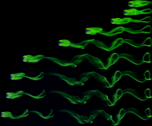
Many previous studies have investigated wake formation behind bluff bodies and some previous research has been undertaken on rolling spheres (Taneda Reference Taneda1965; Stewart et al. Reference Stewart, Leweke, Hourigan and Thompson2008, Reference Stewart, Thompson, Leweke and Hourigan2010a,Reference Stewart, Thompson, Leweke and Houriganb; Rao et al. Reference Rao, Stewart, Thompson, Leweke and Hourigan2011; Verekar & Arakeri Reference Verekar and Arakeri2019). Experimental flow visualisations by Leweke et al. (Reference Leweke, Provansal, Ormiéres and Lebescond1999) captured the wake of an isolated sphere in great detail, showing the division of the re-circulation region into two parallel threads with opposite vorticity, which later combine to form a hairpin-like structure with centre-line mirror symmetry. The photographs also capture the connection between the head of one hairpin vortex to the tail of the previous hairpin vortex, demonstrating the complexity of the wake of an isolated sphere. Houdroge (Reference Houdroge2017) also experimentally visualised the wake of a freely rolling sphere and obtained results in good agreement with numerical predictions. Although these studies have presented flow visualisations at a few distinct  $\overline {Re}$, the present literature lacks a detailed experimental investigation of the wake of a freely rolling sphere, visualising the transitions with increase in $\overline {Re}$. As such, in the present study, we will be presenting detailed visualisations of the wake of a freely rolling sphere, and comparing our results with existing experimental and numerical predictions.
At low  $\overline {Re}$, the flow behind a rolling sphere is steady, remains attached and a fluid re-circulation zone has been observed (Stewart et al. Reference Stewart, Thompson, Leweke and Hourigan2010b). This is analogous to an isolated sphere, where a double threaded wake comprised a counter-rotating vortex pair, as described by Thompson et al. (Reference Thompson, Leweke and Hourigan2021). As $\overline {Re}$ increases, this re-circulation zone grows in size, and the flow becomes increasingly unsteady. Numerical simulations conducted by Stewart et al. (Reference Stewart, Thompson, Leweke and Hourigan2010b) identified that the flow undergoes a transition to unsteady, periodic flow in the range $125 < Re < 150$ for a forward rolling sphere. Rao et al. (Reference Rao, Passaggia, Bolnot, Thompson, Leweke and Hourigan2012) found that this transition occurs at $Re=139$ ( $Re_{c1}$) and further identified a second transition at $Re=192$ ( $Re_{c2}$) where mirror symmetry was broken. Interestingly, Houdroge (Reference Houdroge2017) also found that the first critical transition is strongly dependent on the mass ratio, $\beta =\rho _{s}/\rho _{f}$ (where $\rho _{s}$ and $\rho _{f}$ are the densities of the sphere and fluid, respectively), which acts to delay the onset of unsteadiness in the flow. As $\overline {Re}$ increases further, hairpin vortices are shed into the wake, and in the second transition, centre-plane symmetry of the wake is broken. In simulations by Houdroge (Reference Houdroge2017), significant lateral movement was observed, and vortices were shed at varying orientations. Similar lateral oscillations were observed experimentally by Houdroge et al. (Reference Houdroge, Zhao, Terrington, Leweke, Hourigan and Thompson2023), who attributed these oscillations at lower $\overline {Re}$ to imperfections and dust on the rolling surface. This unsteadiness in the wake leads to VIVs which produce Strouhal numbers ( $St$) ranging between $0.10$ and $0.15$ in line, and $0.05$ cross-slope, for $\overline {Re}<300$ (Houdroge et al. Reference Houdroge, Zhao, Terrington, Leweke, Hourigan and Thompson2023). We will investigate these phenomena further in the present paper.
In this study, we will experimentally investigate the effects of surface roughness on the drag coefficient of spheres, freely rolling without slipping down an inclined plane. We aim to provide experimental evidence that  $\bar {C}_{D}$ is dependent on both the sphere and panel surface roughness, and the effective gap ( $G$) between the panel and sphere can be estimated by assuming an effective gap determined by the surface roughness parameters. However, it should be noted that, due to the logarithmic dependence of $C_{D}$ on gap height (see (2.2)), an order of magnitude change in $G/D$ or surface roughness will only produce relatively small changes in $\bar {C}_{D}$, posing a challenge in establishing the effects of surface roughness on $\bar {C}_{D}$. Nevertheless, we will demonstrate that variations in surface roughness ( $25$-fold change) leads to a change in observed $\bar {C}_{D}$ ( $\approx 10\,\%$), which is well beyond the experimental uncertainty (typically $1\,\%\unicode{x2013}2\,\%$) of the measurements.
Moreover, we demonstrate that the measured drag coefficients are in agreement with the predicted drag coefficient for a smooth sphere and smooth wall, with a gap approximately equal to the root-mean-square (r.m.s.) surface roughness. Our primary focus will be on the inertial flow regime ( $30<\overline {Re}<800$), where the present literature lacks experimental evidence of the dependence of $C_{D}$ on surface roughness. A limited set of experiments of freely rolling foam spheres in air will be conducted for comparison against the results with spheres in water. These results will be used to demonstrate that cavitation (or compressibility) is not a necessary requirement to allow sphere motion. Additional flow visualisations and VIV analysis will also be used to indicate the complexity of the rolling sphere wake and to provide experimental validation of the relative significance of surface roughness and wake formation for the unsteady motion of the sphere. Experimental flow visualisation will be used to validate critical flow transitions that have been observed in previous numerical studies (Rao et al. Reference Rao, Passaggia, Bolnot, Thompson, Leweke and Hourigan2012; Houdroge Reference Houdroge2017). We will demonstrate that the VIV response of a freely rolling sphere is independent of surface roughness, and that results are also in relative agreement with numerical predictions which have been produced assuming a gap between the sphere and plane. This paper is organised as follows. Section 2 describes the problem and the existing analytical solutions and § 3 presents the experimental method. Section 4 presents detailed experimental results of the investigation including flow visualisations and path tracking information together with discussion of observations. Section 5 presents concluding remarks.
2. Problem description
The general case of a sphere of diameter  $D$ rolling down a plane sloped at an angle $\theta$ to the horizontal, considered in this study, is shown in figure 2. The sphere density is denoted by $\rho _{s}$ and the fluid density $\rho _{f}$; typically $\rho _{s}>\rho _{f}$ (negatively buoyant). The coordinate system is attached to the centre of the body and the fluid is stationary with respect to the plane. Once the body reaches a quasi-steady state, it will travel at the time-mean terminal velocity $\bar {U}$ in the $x$ direction and mean angular velocity $\omega$ about the $y$ direction, as indicated in the figure. The $x$ direction is also referred to as the down-slope direction, and the $y$ direction is referred to as the cross-slope direction; $W_{B}$ is the buoyant weight of the body ( $W_{B}={\rm \pi} D^{3} (\rho _{s}-\rho _{f})/6$), and $N$ is the normal reaction at the point of contact between the body and the plane; $\xi$ is the non-dimensional effective gap between the body and the plane imposed by surface roughness, given by $\xi = G/D$. The parameter $\xi$ will be discussed in detail in § 2.2. The parameter $F_{L}$ is the lift force acting on the body, while $T_{y}$ is the total torque about the $y$ axis and $F_{D}$ indicates the total drag force acting on the body.

Figure 2. The schematic free body diagram of the forces acting on a sphere rolling down an inclined plane under the influence of gravity, in a stationary fluid.
Considering the force balance parallel to the plane, the mean drag coefficient of a freely rolling sphere is given by (2.1). Note that the experimentally measured drag coefficient includes both a hydrodynamic component (drag and torque) and contact forces
 \begin{equation} \bar{C}_{D,{exp}} = \frac{4 g \sin(\theta) D (\beta-1)}{3 \bar{U}^{2}}. \end{equation}
2.1. Analytical predictions
Goldman et al. (Reference Goldman, Cox and Brenner1967) provided analytical expressions for the non-dimensional drag force on a sphere, both translating and rotating near a plane wall in Stokes flow, as a function of  $G/D$. Assuming no contact forces between the sphere and the wall, they concluded that a sphere rolling down the plane must slip. Smart et al. (Reference Smart, Beimfohr and Leighton1993) and Houdroge et al. (Reference Houdroge, Zhao, Terrington, Leweke, Hourigan and Thompson2023) assume that static friction forces due to physical contact between surface asperities on both the sphere and the wall cause the sphere to roll without slipping. They present the following expression for the total effective drag coefficient for the Stokes-flow case, which includes both hydrodynamic and contact forces:
 \begin{equation} C_{D,{gap}} = \frac{1}{Re}({-}44.2\log_{10} (G/D) + 34.0). \end{equation}
It should also be noted that, in the derivation of (2.2), a frictional force was required at the contact point to maintain the no-slip boundary condition. Without this force, as stated by Goldman et al. (Reference Goldman, Cox and Brenner1967), the sphere will slip. Therefore, a frictional force at the point of contact is essential for the sphere to roll without slip. Note that the static contact force included in (2.2) does no work on the sphere, and therefore does not reduce the sphere's total kinetic energy. Instead, it transfers the sphere's total kinetic energy between translation and rotation to maintain no slip.
The above equation expresses the contributions of the lubrication flow in the narrow gap between the sphere and the plane to the total drag coefficient, which is referred to as gap-dependent drag ( $C_{D,{gap}}$). The lubrication approach assumes that the gap is much smaller than the sphere diameter ( $G \ll D$), which holds for the spheres considered in the present work.
For non-zero  $\overline {Re}$, there is an additional contribution to the drag coefficient known as wake drag ( $C_{D,{wake}}$), which is approximately independent of $G/D$ (Houdroge et al. Reference Houdroge, Zhao, Terrington, Leweke, Hourigan and Thompson2023; Terrington et al. Reference Terrington, Thompson and Hourigan2023). Houdroge et al. (Reference Houdroge, Zhao, Terrington, Leweke, Hourigan and Thompson2023) provide the following empirical expression for the wake drag coefficient, valid for $5<\overline {Re}<300$, based on numerical simulations performed at $G/D = 0.005$:
 \begin{equation} C_{D,{wake}} = 1.70 - 0.136(\log_{10} Re) - 0.0716(\log_{10} Re)^{2}. \end{equation}
The total drag coefficient is then obtained as the sum of the gap-dependent drag and wake drag
 \begin{equation} C_{D,{pred}} = C_{D,{wake}} + C_{D,{gap}}. \end{equation}
Equation (2.4) is plotted in figure 1 for a fixed  $G/D=10^{-4}$ and shows the same general trend as observed by Carty (Reference Carty1957) for $\overline {Re}<100$. Slight differences between the predictions and experiments are attributed to the influence of gap size, which is not known for Carty's experiments. The experimental results of the present investigation will be compared against the predictions from (2.4), in § 4.4.
2.2. Relationship between gap and surface roughness
A primary aim of the present investigation is to establish the relationship between the effective gap ( $G$) to be used in (2.2)–(2.4), and the surface roughness parameters. Many parameters may be used to describe surface roughness, that vary depending on the application. British Standard Geometric Product Specifications (GPS) – Surface texture: Profile method – Terms, definitions and surface texture parameters, BS ISO 4287:1997 describes these parameters in detail. The most common parameters are mean absolute deviation, r.m.s. and peak roughness ( $R_{a}$, $R_{q}$ and $R_{p}$, respectively).
Based on these roughness parameters, a new non-dimensional relative roughness  $\xi$ will be defined as follows:
 \begin{equation} \xi = \frac{(G)_{effective}}{D} = \frac{(R)_{panel} + (R)_{sphere}}{D}, \end{equation}
where  $\xi$ is the non-dimensional roughness coefficient or relative roughness, $R_{panel}$ and $R_{sphere}$ are the relevant roughness lengths corresponding to the panel and sphere. It is currently unclear what statistical measure of surface roughness best describes the effective gap. In this study, we consider the parameters $\xi _{q}$, $\xi _{a}$ and $\xi _{p}$, based on the r.m.s. roughness ( $R_{q,{panel}}$ and $R_{q,{sphere}}$), mean absolute deviation ( $R_{a,{panel}}$ and $R_{a,{sphere}}$) and peak roughness ( $R_{p,{panel}}$ and $R_{p,{sphere}}$), respectively.
Equation (2.5) assumes that the effective gap ( $G_{effective}$) at the point of contact is the linear summation of the individual roughness values. This is a simplistic approach in approximating the effective roughness, where we have assumed that the sphere and the panel roughness contribute equally to the effective gap between them. This assumption will be discussed in detail in § 4.1.
It is expected that the surface roughness of both sphere and panel will contain multiple scales of roughness, with varying heights and spatial distributions (Galvin et al. Reference Galvin, Zhao and Davis2001; Zhao et al. Reference Zhao, Galvin and Davis2002). The different scales of roughness likely do not contribute equally to determining the effective gap between the sphere and plane. For example, the largest asperities may be too sparsely distributed to provide a significant contribution to the effective gap, while the smallest asperities may be too short to physically contact the opposing wall. Therefore, simple statistical measures of the average roughness properties may be insufficient to fully characterise the effective gap. This is discussed further in § 4.4.
3. Experimental methodology and roughness characterisation
3.1. Experimental set-up
The present experiments were conducted within the Fluids Laboratory for Aeronautical and Industrial Research (FLAIR) at Monash University, Clayton, Australia. Figure 3 shows a schematic diagram of the experimental set-up (not to scale) in the FLAIR laboratory. The water tank used for the experiments measured  $1000\times 500\times 600 \,{\rm mm}^{3}$ ( $L\times W\times H$), with a glass plate of dimensions $800\times 480\times 10 \,{\rm mm}^{3}$ mounted on an adjustable stainless steel frame. The frame was mounted on a base frame, with one end hinged, to allow for the angle of inclination of the top panel and frame to be adjusted using a threaded rod at the other end. The inclination angle varied from $4 ^{\circ }$ to $20 ^{\circ }$. It was observed that, at angles of inclination smaller than $4 ^{\circ }$, the uncertainty of measurements escalated. Other panels made of glass, ceramic and acrylic with varied surface roughness, typically $700\times 300\times 10 \,{\rm mm}^{3}$ in size, were also used for the experiments. These panels were placed atop the existing glass panel and clamped down to limit relative movement. The properties of the panels and spheres used during the experimental process are described in tables 1 and 2.

Figure 3. Experimental set-up of the water tank at the FLAIR Laboratory, Monash University.
Table 1. Panel types used as inclined planes are detailed here. Max. deviation is the maximum absolute deviation of surface height measurements from the mean plane. Max. gradient is the maximum cross-slope gradient over a minimum cross-slope measurement distance of 50 mm.

Table 2. Specifications of spheres used for experimental evaluation are given in the table above. Each diameter corresponds to a set of eight individual spheres, and three measurements of each sphere were obtained to calculate the values presented above. The mean values of diameter including the error for each set are shown above. Refer to Appendix A for details of the uncertainty analysis.

The flatness of the panels used was estimated by measuring the surface height variation based on 48 equally spaced grid points on the surface of the panels. Panels were placed on a cast iron surface plate (manufactured by Wing Industries, Australia; Grade D), machined and installed to be horizontally levelled, which was used as a reference surface. A metric dial indicator (manufactured by Mitutoyo, Japan; accuracy =  $0.01$ mm) and an arm were used to measure the height of the rolling surface of the panel, from which a mean plane was obtained. Two parameters have been used in table 1 to describe the flatness of the plates. Max. deviation (mm) describes the maximum absolute deviation of surface height measurements from the mean plane. Max. gradient is the maximum cross-slope gradient over a measurement distance of $50$ mm. The smallest angle of inclination used for experiments was $4 ^{\circ }$, which yields a maximum gradient of ${\approx }7\,\%$ down the slope. Comparing this with the maximum cross-slope gradient of $0.3\,\%$ for the acrylic panel, we can conclude that the non-flatness of the panel is negligible compared with the down-slope angle of inclination of the panels.
A waterproof digital inclinometer (model: DWL 280, Digi-Pas US, accuracy =  $0.05^{\circ }$) was used to measure the angle of the panel with respect to the horizontal axis. Water temperature was initially measured using a water-resistant digital thermometer (Mextek, accuracy = $0.1\,^{\circ }$C). During the second stage of testing, a residual temperature device configured for the temperature range of 10–40 $^{\circ }$C, for an output voltage range of 0–10 V, was used (ECEFast RTD PT100, Accuracy = 0.001 V). These measurements allowed for the calculation of water viscosity and density in accordance with the International Association for the Properties of Water and Steam (IAPWS) Formulation 2008 for the Viscosity of Ordinary Water Substance (reference IAPWS 2008).
The spheres were pre-soaked under the water level, and air bubbles were manually removed using vibration and stirring. Then the spheres were placed atop the inclined plane, at a collection port and released, carefully ensuring minimum disturbance to the water surface. Following any perturbation of the water, a minimum of 2 min was allowed to ensure that the water was reset to rest prior to any further measurements. The water tank was also cleaned regularly to ensure that any dust or fibres were not deposited on the surface of the panels. It was noted that the presence of small air bubbles, fibres or dust deposited on the panel surface significantly affected measurements. As such, all attempts were made to ensure that the presented results were void of these errors.
The rolling sphere velocities were calculated by measuring the time taken to travel a fixed distance. The spheres were allowed to roll a minimum of  $20 D$ prior to starting the measurements. Initially, a stopwatch was used to measure the time taken to travel $200$ mm distance atop the removable panel ( $70\,\%$ of data). In the second half of the project, a new system incorporating three laser-based object detectors was developed to improve the accuracy and efficiency of these measurements (see figure 4, $30\,\%$ of data). The uncertainty analysis presented in Appendix A considers errors from both types of measurements. The results presented in this paper include both sets of data. Each measurement presented in § 4.1 represents the mean values of eight individual runs recorded using a set of spheres with same density and diameter. In addition, spot checks were done at random locations to ensure the data were repeatable, even under different fluid temperatures.

Figure 4. Laser set-up used to measure sphere velocity.
Table 2 presents the uncertainty of the sphere diameter in each set of spheres, which was typically less than  $1\,\%$. The uncertainty in sphere diameter was used to estimate deviations in sphericity. Given that the uncertainties in the diameter of acrylic and cellulose acetate (CA) spheres were generally below $1\,\%$, it was assumed that deviations in the sphericity of spheres could be neglected.
To minimise any distortion of spheres and panels due to water absorption (mainly acrylic, which is known to absorb water), they were removed from the water tank outside of measurement windows and dried regularly.
A set of preliminary tests at angles of inclination in the range  $4^{\circ }\unicode{x2013}20^{\circ }$ using a subset of the spheres, covering a range of $\overline {Re} (40\unicode{x2013}900)$ were carried out to test whether the sphere slips in our experiments. A marker was placed on the sphere surface and the sphere was recorded with a digital camera. The estimated rotational velocity was compared against the measured translational velocity and no significant deviation between translational and rotational velocities ( ${<}1\,\%$) was observed. Therefore, any slip between the sphere and the wall, if present, is negligible. In addition, detailed experiments conducted by Wardhaugh & Williams (Reference Wardhaugh and Williams2014) and Tee (Reference Tee2018) observed no slip below ${\approx }25 ^{\circ }$ for spheres rolling on a glass plate in water. This evidence, coupled with our own preliminary measurements, was sufficient to conclude that the no-slip condition is met under the present experimental conditions.
3.2. Surface roughness measurements
An optical profilometer (Bruker Contour GT-I) located at the Melbourne Centre for Nanofabrication in the Victorian Node of the Australian National Fabrication Facility was used to obtain non-contact surface roughness measurements of all the spheres and panels. Roughness measurements were obtained under 50 times magnification using the vertical scanning interferrometry method. Vertical scanning interferrometry utilises a broad band light source and is accurate when measuring typically rough surfaces. Tables 3 and 4 present the measured values.
Table 3. Measured surface roughness values of panels. Values presented are the arithmetic mean of five individual measurements. The measurement area of each presented measurement is  $0.25\times 0.25\,{\rm mm}^{2}$ (12 measurements under $50 \times 1$ magnification joined together).

Table 4. Measured surface roughness values of spheres. Values presented are arithmetic mean of five individual measurements of five separate spheres, of the same diameter. The measurement area of each presented measurement is  $0.3\times 0.3$ mm $^{2}$ for all diameters (12 measurements under $50\times 1$ magnification joined together), leading to percentage measurement areas ranging from $0.23\,\%$ for $D=3.44$ mm to $0.02\,\%$ for $D=11.49$ mm. All measurements were corrected for sphere curvature prior to obtaining roughness statistics.

Figure 5 depicts the surface roughness measurements of two panels and two spheres used for experiments. The surface roughness profiles of the glass panel in figure 5(a) range from  $40$ to $60$ nm while frosted glass in figure 5(b) has significantly taller asperities reaching as high as $5\,\mathrm {\mu }$m. Similarly, the asperities on both spheres indicated in figure 5(c,d) also contain a sparse distribution of asperities taller than $1\,\mathrm {\mu }$m, with the majority of asperities being around the $0.5\,\mathrm {\mu }$m range. A clear observation from these images is the sparse distribution of very tall asperities. Captions of tables 3 and 4 contain additional information regarding the measurement techniques used.

Figure 5. Surface roughness profiles obtained using the optical profilometer, under  $50{\times }$ magnification. (a)Glass panel, (b) frosted glass panel, (c) 3.95 mm diameter acrylic sphere, (d) 6.35 mm diameter CA sphere.
4. Results and discussion
4.1. Measured Reynolds number vs drag coefficient data in water
Based on the experimental set-up and methodology noted in § 3.1, measurements of  $\bar {C}_{D}$ and $\overline {Re}$ were obtained for $30<\overline {Re}<800$, corresponding to 13 different diameter spheres rolling on four separate panels. Figure 6(a) shows all of the data gathered, with the figure legend indicating the marker shapes corresponding to sphere diameters. Figure 6(b) presents the same data on a log–log scale, with the legend showing the marker colours corresponding to panel types. The data indicate a similar trend to those of previous studies (i.e. $1/Re$ trend, as observed by Carty Reference Carty1957; Garde & Sethuraman Reference Garde and Sethuraman1969; Jan & Chen Reference Jan and Chen1997). Results of Carty (Reference Carty1957) are plotted in figure 6 for comparison. There is a notable variation of $\bar {C}_{D}$ with panel type and sphere diameter at a given $\overline {Re}$ for $\overline {Re}<200$; at $\overline {Re}=100$ this observed deviation is of the order of $10\,\%$.

Figure 6. Variation of  $\bar {C}_{D}$ with $\overline {Re}$ for a sphere rolling down an inclined plane. Markers corresponding to individual sphere diameters are as indicated in the legend of figure 6(a) and the marker colours correspond to the panel as indicated in figure 6(b). (a) All data points, $\overline {Re} = 30\unicode{x2013}800$ range; (b) $\overline {Re} = 30\unicode{x2013}1000$ range in log–log scale.
A distinctly higher  $\bar {C}_{D}$ for the three larger CA spheres ( $D=6.89$ mm, $9.74$ mm and $11.49$ mm) is seen in figure 6. Generally, these spheres follow a separate $\bar {C}_{D}$ vs $\overline {Re}$ trend compared with the other spheres investigated. Additionally, in figure 9, we observe a distinct increase in $\bar {C}_{D}$ for the $D=6.89$ mm CA sphere, for all four panels considered. At this stage, we cannot quantitatively explain this jump in $\bar {C}_{D}$ for the larger CA spheres. However, the surface finish of these larger spheres (matte finish) was distinct from the smaller spheres (shiny finish). The matte finish spheres contained a higher density of larger peaks and valleys. Despite the distinct surface finishes, the roughness statistics of both types of spheres are nominally similar (table 4, $R_q \approx 0.5\, \mathrm {\mu } {\rm m}$). A plausible explanation, to be investigated in more detail in the future, is that the higher $\bar {C}_{D}$ is due to an increased rolling resistance induced by the higher density of the taller peaks. Mechanisms concerning rolling resistance are discussed further in § 4.4.3.
The results of foam spheres are not included in figure 6, and are presented in § 4.2.
Upon closer examination of the data for  $\overline {Re}<300$, multiple trend lines are observed as the panel surface roughness and sphere diameter are varied, as was observed by Houdroge et al. (Reference Houdroge, Zhao, Terrington, Leweke, Hourigan and Thompson2023). This variation of $\bar {C}_{D}$ with panel type is clearly observed in figure 6(b). Figure 7 presents the variation of $\bar {C}_{D}$ with $\overline {Re}$ ranging from $50<\overline {Re}<120$, in which two least-squares lines of the form $a+b/Re$ have been fitted through the data points corresponding to the two panels used. The $r^{2}$ values, indicating goodness of fit of the curves, are approximately $0.9$, indicating a good fit. The deviation of $\bar {C}_{D}$ with the change in panel roughness is highlighted in this figure. There is an approximately $10\,\%$ increase in $\bar {C}_{D}$ at $\overline {Re}=100$ between the frosted glass panel and the glass panel (which corresponds to an 80 times decrease in panel $R_{a}$ roughness). The increase in $\bar {C}_{D}$ with a decrease in roughness (or $\xi =G/D$) can be attributed to the increase in the gap drag component with a decrease in gap height, as was predicted in (2.4).

Figure 7. Variation of  $\bar {C}_{D}$ with $\overline {Re}$ for the two individual panels, with least-squares lines fitted through each panel. Marker shapes correspond to sphere diameter, as indicated in the legend of figure 6(a). The $R_{q}$ roughness of the two panels are as follows: frosted glass panel; $2.33\,\mathrm {\mu }$m, glass panel; $0.029\,\mathrm {\mu }$m. Error bars indicate combined bias error and random error. Refer to Appendix A for details on error analysis.
This increase in  $\bar {C}_{D}$ with a decrease in panel surface roughness is further highlighted in figure 8, where the sphere diameter was fixed ( $D=5.86$ mm) while the panel roughness was varied. The individual variations of $\overline {Re}$ vs $\bar {C}_{D}$ are clearly observed in this figure.

Figure 8. Variation of  $\bar {C}_{D}$ with $\overline {Re}$ for a fixed diameter, $D=5.86$ mm. Data for three individual panels, with least-squares lines fitted through each panel are shown. Error bars indicate bias error only.
Upon even further examination of figure 7, what initially appears to be scatter around curves fitted for a panel, more trend lines indicating variation in  $\bar {C}_{D}$ vs $\overline {Re}$ for specific diameters are observed. Figure 9 presents the data separated by panel roughness, with least-squares lines of the form $a+b/Re$ fitted through the data corresponding to individual diameters. A subset of the data is presented in this figure to highlight the variation of $\bar {C}_{D}$ with sphere diameter. It is observed that variations in $D$ with a fixed panel surface roughness lead to variations in measured $\bar {C}_{D}$. As indicated in figures 9 and 10, an increase in sphere $D$ leads to an increase in $\bar {C}_{D}$. This observed increase is greater at lower $\overline {Re}$ than at higher values; however, the observed variations still maintain the overall $1/Re$ behaviour. A similar observation was made by Houdroge et al. (Reference Houdroge, Zhao, Terrington, Leweke, Hourigan and Thompson2023) on the variation of $C_{D}$ with the sphere diameter. These observations provide further evidence that the relative roughness ( $\xi$) is dependent on the panel roughness, the sphere roughness and also the sphere diameter, as we have assumed in (2.5). For each $\xi$, we observe a separate $\bar {C}_{D}$ vs $\overline {Re}$ relationship.

Figure 9. Variation of  $\bar {C}_{D}$ with $\overline {Re}$ for the four panels used for experimentation in the range $100>\overline {Re}>300$. Least-squares lines of the form $a+b/Re$ have been fitted through data that correspond to individual diameters of the spheres used. Error bars indicate bias error only. (a) Glass panel, (b) acrylic panel, (c) ceramic panel, (d) frosted glass panel.

Figure 10. Comparison of  $\bar {C}_{D}$ vs $\overline {Re}$ between acrylic and CA spheres, of similar diameters, rolling on a glass panel against analytical prediction (2.4). (a) Two acrylic spheres, (b) two CA spheres.
Figure 10 presents a comparison between the experimentally measured drag coefficients, and the drag coefficients predicted using (2.4) under the assumption  $G/D = \xi _{q}$. Figure 10(a) shows that the measured $\bar {C}_{D}$ is in good agreement with analytical predictions for acrylic spheres, and therefore $\xi _{q}$ is a suitable estimate of the effective gap. However, for CA spheres (figure 10b), analytical predictions assuming $G/D = \xi _{q}$ underestimate $C_{D}$, particularly at lower $\overline {Re}$ ( $\overline {Re}<100$). Nevertheless, at higher $\overline {Re}$, a better agreement between analytical predictions and experimental measurements is observed. This observation is further supported through data presented in §§ 4.3 and 4.4, where the effective values of $\xi$ required to match the predicted drag (2.4) to the experimental measurements are closer to the measured $\xi _{q}$ for acrylic spheres but are below the measured $\xi _{q}$ for CA spheres. Therefore, the assumption $G/D = \xi _{q}$ is applicable to acrylic spheres, but not CA spheres. As discussed in § 2.2, simple roughness statistics such as $R_{q}$ may not capture the complexities of the various scales of surface roughness that contribute to the effective gap. We also note that the effective $\xi$ required to match the predictions and measurements is still of the same order of magnitude as the measured $\xi _q$ for CA spheres. These issues are discussed further in §§ 4.3 and 4.4. For now, we assume $G/D = \xi _{q}$ is a valid approximation, at least to within one order of magnitude.
As discussed previously in § 1, Goldman et al. (Reference Goldman, Cox and Brenner1967) dismissed surface roughness as a possible explanation for the disparity between the analytical prediction and experimental data. However, based on the data observed in figures 6–10, there is a clear correlation between surface roughness and the measured  $\bar {C}_{D}$, and therefore surface roughness is at least partially responsible for allowing the sphere to move. Moreover, the $G/D$ required to match the experimental measurements and the predicted drag using (2.4) is of the same order of magnitude as the r.m.s. surface roughness ( $\xi _q$), supporting our hypothesis that surface roughness introduces an effective hydrodynamic gap between the sphere and the wall.
4.2. Measured Reynolds number vs drag coefficient data for foam spheres in air
Goldman et al. (Reference Goldman, Cox and Brenner1967) tentatively suggest that cavitation, rather than surface roughness, is responsible for the motion of the sphere. This suggestion is supported by experimental observation of cavitation bubbles appearing close to the point of contact between the body and the plane for heavy bodies in highly viscous fluids (Prokunin Reference Prokunin2003; Ashmore et al. Reference Ashmore, Del Pino and Mullin2005; Seddon & Mullin Reference Seddon and Mullin2006). Cavitation has been observed primarily in the Stokes regime, where the viscous forces are greater than the inertial forces. We have concentrated our efforts so far on the motion of bodies at somewhat higher  $\overline {Re}$ ( ${>}30$), and have not observed any cavitation bubbles during our experiments in water for acrylic and CA spheres ( $\beta = 1.2, 1.3$).
To further evaluate the role of cavitation in the drag experienced by rolling spheres, experimental measurements were obtained for foam spheres rolling down an inclined surface in air. If cavitation, rather than surface roughness, were responsible for determining the effective gap, we would expect large differences in the measured drag coefficients between air and water, given that cavitation does not occur in air.
Figure 11 depicts the obtained  $\bar {C}_{D}$ vs $\overline {Re}$ variation for foam spheres rolling down an inclined plane in air on acrylic and frosted glass panels. The results of acrylic spheres of similar diameters rolling on the same panels in water are also plotted for comparison. Experiments performed in air, where cavitation cannot occur, display the same trends and values of $\bar {C}_{D}$ as those performed in water. The agreement between the results of measurements conducted in air and in water suggests that cavitation does not affect the motion of the sphere, at least for the experimental parameters considered in this study.

Figure 11. Variation of  $\bar {C}_{D}$ with $\overline {Re}$ for a foam sphere rolling down in inclined surface in air. (a) Foam spheres on acrylic panel, (b) foam spheres on frosted glass panel.
The surface roughness of foam spheres is larger than that of the acrylic and CA spheres, as seen in table 4. However, figure 12 shows that the measured  $\bar {C}_{D}$ values are similar to those of the other spheres, and follows the general $\bar {C}_{D}$ vs $\xi _q$ trend.

Figure 12. Variation of  $\bar {C}_{D}$ with $\xi _{q}$ for three fixed $\overline {Re}$. Values of $\bar {C}_{D}$ at specific $\overline {Re}$ values were calculated using linear interpolation of nearest neighbours. The $C_{D}$ predictions from (2.4) are also plotted for comparison with experimental results. Results of foam spheres rolling in air are also plotted in the same figure.
Terrington et al. (Reference Terrington, Thompson and Hourigan2022) present a general model for predicting the motion of the sphere in both cavitating and non-cavitating flows. They consider three dynamic regimes: contacting motion without slip; contacting motion with slip; and non-contacting motion. Contacting motion with slip occurs at low inclination angles, with the sphere transitioning first to the slip regime, and then to the non-contacting regime, as the inclination is increased. The present study considers angles of inclination below  $20^{\circ }$, both in water and air, and no slipping was observed. Therefore, the results of the present study all fall in the ‘contacting motion without slip’ regime. For a different set of experimental parameters, cavitation may be responsible for determining the effective gap.
4.3. Variation of drag coefficient with surface roughness
This subsection investigates the effects of the r.m.s. surface roughness ( $\xi _{q}$) on the mean drag coefficient ( $\bar {C}_{D}$). Figure 12 plots the variation of the measured $\bar {C}_{D}$ vs $\xi _{q}$ for three constant values of $\overline {Re}$ ( $70,100,150$). Here, $\xi _{q}$ was calculated using (2.5) based on the r.m.s. roughness measurements presented in tables 3 and 4. The $\bar {C}_{D}$ values corresponding to each $\overline {Re}$ were calculated using linear interpolation from the nearest neighbouring $\overline {Re}$. Some scatter in data is observed at each $\overline {Re}$, introduced by the uncertainty of both $R_q$ ( ${\approx }5\,\%$) and interpolated $\bar {C}_{D}$ ( ${\approx }2\,\%$) measurements. The approximation of $G$ using $R_q$ roughness will also introduce an error, which is more prominent for the CA spheres, and at lower $\overline {Re}$, as discussed in § 4.4.
A line of best fit of the form  $a + b\log (\xi )$ has been fitted through the experimental data to indicate the general trend of decreasing $\bar {C}_{D}$ with increasing $\xi _q$. Light shading around curves indicates the uncertainty of the fitted curve, quantified by constructing a $95\,\%$ confidence interval about the regression line, assuming that errors are normally and randomly distributed. The $r^{2}$ values of the curve fits were $\approx 0.4$, indicating that, while variations in $R_q$ roughness account for some of the variation in $\bar {C}_{D}$, it is not accurate for all cases (see § 4.4.2 which discusses these issues further). The results for foam spheres in air are also plotted in the figure. Note that foam data (which have larger uncertainties) have been excluded from the curve fits.
At  $\overline {Re} = 70$, there is approximately a $9\,\%$ reduction in $\bar {C}_{D}$ as $\xi _{q}$ is increased from $4\times 10^{-5}$ to $1\times 10^{-3}$ ( $25$-fold increase). At $\overline {Re} = 100$ and $150$, the decrease in $\bar {C}_{D}$ for the same change in $\xi _{q}$ is approximately $10\,\%$. The absolute reductions of $\bar {C}_{D}$ at the same $\overline {Re}$ are approximately $0.42,0.36$ and $0.28$, respectively. The experimental uncertainty of measurements of $\bar {C}_{D}$ is typically $\approx 2\,\%$ (see Appendix A). The measured reduction in $\bar {C}_{D}$ for a $25$-fold increase of roughness is well above the experimental uncertainty of the $\bar {C}_{D}$ measurements. This observation, coupled with the relative agreement between the effective $\xi$ and roughness statistics discussed in § 4.4, support the present hypothesis that surface roughness provides the gap required by lubrication theory, and is dependent on both the sphere and panel roughnesses.
The increase in  $\bar {C}_{D}$ with decreasing $\xi _{q}$ is consistent with our hypothesis that the effective gap is governed by the height of surface asperities. Figure 12 includes predicted drag coefficients using (2.4) (predictions from Houdroge et al. Reference Houdroge, Zhao, Terrington, Leweke, Hourigan and Thompson2023), under the assumption $G/D = \xi _{q}$ at $\overline {Re} = 70, 100$ and $150$. The computational and analytical solutions correctly predict that $\bar {C}_{D}$ increases as $\xi _{q}$ is decreased; however, they marginally underestimate $\bar {C}_{D}$ compared with the present experimental results. The discrepancy between the predicted and measured $\bar {C}_{D}$ indicates either that the effective gap is smaller than $\xi _{q}$, or that there is some additional source of drag that has not been accounted for in our analysis.
A possible source of this additional drag could be the rolling resistance due to surface roughness. This is discussed further in § 4.4.3.
The dependence of  $\bar {C}_{D}$ on $\xi$ is limited to low $\overline {Re}$ values ( $\overline {Re}<500$). In figure 12 we observe that the $\overline {Re}=150$ curve is flatter compared with the smaller $\overline {Re}$. The value of $\bar {C}_{D}$ decreases marginally when $\overline {Re}$ is increased further, although the differences in $\xi$ remain unchanged. This observation can be explained using (2.4). The parameter $\xi _{q}$ affects only the gap-dependent drag ( $C_{D,{gap}}$), and not the wake drag ( $C_{D,{wake}}$). The gap-dependent drag is proportional to $1/Re$ (2.2), and therefore becomes negligible at high $\overline {Re}$. The wake drag coefficient remains $O(1)$ as $\overline {Re}$ is increased (Houdroge et al. Reference Houdroge, Zhao, Terrington, Leweke, Hourigan and Thompson2023), and therefore dominates the total drag at high $\overline {Re}$. Since the wake drag does not depend on $\xi _{q}$, the sensitivity of $\bar {C}_{D}$ to $\xi _q$ decreases as $\overline {Re}$ is increased.
Referring to the Carty (Reference Carty1957) data in figure 1,  $\bar {C}_{D}$ remains relatively constant at $\bar {C}_{D}\approx 1$ in the range $10^{3}<\overline {Re}<10^{4}$. At these high $\overline {Re}$, the total $\bar {C}_{D}$ is almost certainly dominated by wake drag, and therefore $C_{D,{wake}}$ is approximately constant for high $\overline {Re}$. We also note a similar trend in behaviour for a sphere in free fall (Rouse Reference Rouse1946), which does not contain either gap or contact forces. It should be noted that, unlike the case of a free-falling sphere, the presence of the panel impacts the wake structures generated, and therefore the converged $\bar {C}_{D}$. That is, for a free-falling sphere, $\bar {C}_{D} \approx 0.4 (10^{3}<\overline {Re}<10^{4})$ (Rouse Reference Rouse1946), while for a freely rolling sphere, $\bar {C}_{D}\approx 1 (10^{3}<\overline {Re}<10^{4})$; the difference is attributed to the effects of the plane on the near wake and wake structures generated by the sphere.
The above observations support our hypothesis that the surface roughness of both the sphere and the panel results in an effective gap between the sphere and the wall when the two surfaces are in contact. The mean drag coefficient can be estimated by assuming the gap is equal to the combined r.m.s. roughness of both the sphere and the wall ( $\xi _{q}$).
4.4. Roughness analysis
So far, we have been assuming the effective gap  $\xi$ is equal to the combined r.m.s. roughness of the sphere and panel ( $\xi _{q}$). As discussed previously (§ 2.2 and briefly in § 4.1), simple statistical measures such as $R_q$ may not capture the various scales of surface roughness. To investigate these effects further, we consider four cases in detail – two acrylic spheres with $D=3.95$ mm and $D=4.71$ mm and two CA spheres with $D=3.94$ mm and $D=4.87$ mm – rolling on a glass surface. Since the roughness of the glass panel is much smaller than that of the sphere by a factor of 10, we expect the gap will be dominated by the roughness of the sphere.
4.4.1. Relationship between effective  $\xi$ and $R_{q}$


We define the effective  $\xi (=G_{eff}/D)$ as the $G/D$ required to match the predictions of (2.4) with the experimental measurements. These effective $\xi$ are shown in figure 13 for the four spheres, alongside the measured r.m.s. roughness ( $R_{q}$), mean roughness ( $R_{a}$) and peak roughness ( $R_{p}$) of the sphere, normalised by the sphere diameter. Light coloured shading indicates one standard deviation error of the roughness measurements. As observed in the figure, $R_p/D$ values are generally larger and overestimate the gap height. Though $R_a/D$ and $R_q/D$ are similar in magnitude, $R_a/D$ underestimates the gap for the two acrylic spheres. As such, $R_q$ roughness was chosen as the roughness metric that best correlates with the effective $\xi$.

Figure 13. Effective  $\xi$ vs $\overline {Re}$ for four spheres rolling on a smooth glass panel. The measured roughness parameters of the spheres are plotted in the figure. Error bands shown by light shading indicate one standard deviation error of roughness parameters. Panels show (a) $D=3.95\,{\rm mm}$ acrylic sphere, (b) $D=3.94\,{\rm mm}$ CA sphere, (c) $D=4.71\,{\rm mm}$ acrylic sphere, (d) $D=4.87\,{\rm mm}$ CA sphere.
In all four cases, we observe that the effective  $\xi$ increases with increasing $\overline {Re}$, before reaching an approximately constant value. This approximately constant value is also shown in the figure as $\xi _{mean}$. The fixed gap height at higher $\overline {Re}$ is of the same order of magnitude as the sphere $R_{q}/D$ for acrylic and below $R_{q}/D$ for CA spheres. This figure indicates that $R_{q}/D$ is an excellent approximation for $\xi$ for the acrylic sphere above $\overline {Re}=50$ for the $D=3.95$ mm sphere and above $\overline {Re}=80$ for the $D=4.71$ mm sphere. However, the $R_{q}/D$ for the CA spheres overestimates the gap by a factor of $2$–
$2$– $3$ for both CA spheres. The parameter $R_{a}/D$ provides marginally better agreement for the two CA spheres, but the difference is too small to conclude that $R_{a}/D$ is a better metric. However, it is promising that the effective $\xi$ is of the same order of magnitude as $R_q/D$ (or $R_{a}/D$) roughness, for all four cases considered here, highlighting that roughness likely provides a satisfactory explanation for the gap required by lubrication theory, while also allowing solid-to-solid contact.
Figure 13 also indicates that the effective  $\xi$ is smaller at low $\overline {Re}$, and increases with $\overline {Re}$. The increase in the effective $\xi$ with $\overline {Re}$ is in general agreement with the predictions of Galvin et al. (Reference Galvin, Zhao and Davis2001) and Zhao et al. (Reference Zhao, Galvin and Davis2002). They considered two scales of roughness – a dense covering of small asperities, and a sparse covering of large asperities. Their model predicts an effective gap close to the height of the small asperities at low speeds, but which increases towards the height of the large asperities at high speeds. It should also be noted that the present combined analytical and numerical solution ignores the effects of rolling resistance. Given that rolling resistance due to collisions between surface asperities (see § 4.4.3) will be a function of the plane normal component of the buoyant weight of the sphere ( $W_{B}g\cos (\theta )$) (see figure 2), we can expect this to be more prominent at lower angles of inclination ( $\theta$), hence lower $\overline {Re}$. This might provide a reasonable explanation for the observed divergence of effective $\xi$ at low $\overline {Re}$; however, this analysis is beyond the scope of the present study.
4.4.2. Comparison of surface textures of the two materials
From figure 13, we see that, for acrylic and CA spheres of approximately equal diameter, the acrylic sphere has a larger effective  $\xi$, while the CA sphere has a marginally larger r.m.s. roughness ( $R_{q,{sphere}}/D$). Therefore, the r.m.s. roughness alone is not sufficient to fully characterise the effective gap. To explain this difference, figure 14(a,b) compares the surface textures of the two materials corresponding to $D=3.95$ mm acrylic and $D=3.94$ mm CA spheres. Two-dimensional excerpts of the surface roughness measurements are shown in figure 14(c,d). Sections A–A were selected to represent sections with $R_{q}$ similar to that of the mean $R_{q}$ of the spheres, as indicated in table 4 and figure 13. The geometry of the sphere is also indicated for visualisation.

Figure 14. Detailed review of  $D=3.95$ mm acrylic and $D=3.94$ mm CA spheres. (a) Three-dimensional surface of $3.95$ mm acrylic sphere. Measurement $R_{q}=0.40$. (b) Three-dimensional surface of $3.94$ mm CA sphere. Measurement $R_{q}=0.54$. (c) Section A–A of (a). Two-dimensional surface profile of $D=3.95$ mm acrylic sphere. (d) Section A–A of (b). Two-dimensional surface profile of $D=3.94$ mm CA sphere.
The surface textures of both acrylic and CA spheres are remarkably different. The acrylic sphere contains two clearly distinct scales of asperities: small asperities which are typically in the range  $0.1\unicode{x2013}0.5\,\mathrm {\mu }$m in height that densely cover the sphere, and a sparse distribution of large asperities in the range $2$–
$2$– $10$
$10$  $\mathrm {\mu }$m in height (10 $\mathrm {\mu }$m asperities are not shown in the figure). The CA sphere contains a single scale of asperities that are typically between $0.5$ and $1\,\mathrm {\mu }$m in height, but which can be up to 5 $\mathrm {\mu }$m in height. The CA sphere also contains large valleys, which are of a similar depth to the height of the asperities, while the acrylic does not contain large valleys.
The  $R_{q}$ roughness of the $D=3.95$ mm acrylic spheres was measured to be $0.40$ $\mathrm {\mu }$m while for the CA sphere it was $0.60\,\mathrm {\mu }$m, and these are also indicated in figure 14(c,d) for comparison. The measured $R_{q}$ roughness of CA is approximately $50\,\%$ larger than that of acrylic. This is due to the CA sphere containing a high density of moderately large ( $0.5$– $1\,\mathrm {\mu }$m) asperities, including both bumps and valleys. While the acrylic sphere contains some very tall asperities, these are balanced out by a large proportion of the sphere containing only small asperities, leading to a smaller overall $R_{q}$. The mean effective gap (mean $G$) calculated from figure 13 is also shown in figure 14(c,d). This indicates the effective average gap required to match the predicted $\bar {C}_{D}$ with experimental measurements. While the $R_{q}$ roughness of the CA sphere is greater than that of the acrylic sphere, the effective gap of the CA sphere is below that of the acrylic sphere. For both acrylic and CA, the heights of the surface asperities are not uniform across the surface. There are many regions on the sphere's surface where the size of asperities – and therefore the minimum possible gap – is well below both mean $G$ and $R_{q}$. Similarly, there are many regions where the local asperities are taller than both mean $G$ and $R_{q}$.
Therefore, our assumption that surface roughness produces an effective gap is consistent with the detailed measurements of the surface profiles for both acrylic and CA. The effective gap is larger than the smallest asperities, but smaller than the largest asperities, as is to be expected. Simple statistical measures, such as  $R_{q}$, can approximately indicate the effective gap. However, $R_{q}$ does not consider several important factors, such as the spatial distribution of asperities, and the existence of multiple scales of surface roughness. In the case of acrylic, the effective gap and the r.m.s. roughness agrees quite well. However, this does not hold for all materials.
4.4.3. Other considerations
As discussed in § 2.2, although the heights of surface asperities may vary (approximately from 0.1 to  $10\,\mathrm {\mu }$m for the spheres under consideration), it is likely that not all the scales of roughness will contribute equally to determining the effective gap. Moreover, the effective gap may depend on the speed of the sphere as well. As observed in figure 13, at lower rolling speeds (low $\overline {Re}$) the effective gap is small but gradually increases with $\overline {Re}$. Under the two-scale model of Galvin et al. (Reference Galvin, Zhao and Davis2001) and Zhao et al. (Reference Zhao, Galvin and Davis2002), the effective gap is predominantly determined by the smallest scale of roughness at low speeds. At high speeds, however, the sphere does not have time to fall below the height of the large asperities, and therefore the effective gap is dominated by the height of the largest asperities. We note, however, that the effective gap presented in figure 13 becomes independent of $\overline {Re}$ at an effective gap well below the height of the tallest asperities. For instance, the $D=3.95$ mm acrylic sphere contains asperities greater than $2\,\mathrm {\mu }$m, corresponding to $\xi =0.0005$. However, the effective $\xi$ reaches a maximum value of $\xi =0.0001$. We tentatively suggest that the large asperities do not cover enough of the sphere's surface to maintain an effective gap equal to the height of the large asperities. However, it is likely that these large asperities will make some contribution to the overall effective gap since the effective gap is generally larger than the height of the small asperities.
As mentioned in § 4.3, a possible source of additional drag could be rolling resistance, which has not been accounted for in the analytical derivations. Analytical derivations assumed a plane normal contact force at the point of contact between the sphere and the plane. In reality, the contact force is replaced by a contact area, and energy may be dissipated at this contact region. Mechanisms contributing to energy dissipation, which are typically considered as rolling resistance, cover an extensive area of research. Bikerman (Reference Bikerman1949) and Halling (Reference Halling1958) highlight some of these mechanisms, a few of which are noted here: continuous collisions, elastic deformation, capillary action, hysteresis effects, inter-facial slip and molecular adhesion. At constant rolling velocity, the rolling resistance due to surface roughness can be assumed to be constant, and will increase with increasing speed as observed by Cross (Reference Cross2015, Reference Cross2016) for a rolling sphere on a hard surface. Cross (Reference Cross2016) presents a theoretical model to estimate the rolling resistance due to surface asperities on a rolling sphere, with an unknown parameter to be determined empirically. Some disagreement between theoretical and experimental results was also observed. Moreover, their model considers spheres rolling in a vacuum and does not consider lubrication forces in the gap region, nor fluid forces in general. Experimental measurements of rolling resistance by Halling (Reference Halling1958) and Cross (Reference Cross2016) for hard spheres rolling in air are typically around  $0.0001\unicode{x2013}0.001$. Assuming a similar range of rolling resistances for our spheres, as a drag coefficient this contribution would likely be of the order of $0.0005\unicode{x2013}0.5$. However, without an accurate analytical model that predicts the effects of rolling resistance with $\xi$ (or roughness), we cannot determine the exact contribution of the rolling resistance to $\bar {C}_{D}$. The construction of such a model is beyond the scope of the present study and is recommended for future work. We anticipate that the rolling resistance will increase as $\xi _{q}$ is increased.
Summarising the results of this section, the effective gap required to match the predicted and experimental drag coefficients is greater than the smallest surface asperities, but less than the largest asperities, consistent with our hypothesis that the effective gap is due to the surface roughness. However, simple statistical averages such as r.m.s. roughness only approximate the effective gap, since these averages do not account for the many different scales of surface roughness that are present. Further analysis of surface roughness against  $\overline {Re}$ is required to understand which scales of roughness are critical at specific $\overline {Re}$.
4.4.4. Rolling paradox
Although we have argued that physical contact between surface asperities results in an effective gap, we note that lubrication theory still requires an infinite pressure at the point where two asperities come into contact (Thompson et al. Reference Thompson, Leweke and Hourigan2021). One possible explanation for the phenomenon could be non-continuum flow. Although previously dismissed by Goldman et al. (Reference Goldman, Cox and Brenner1967), arguing that the effects of surface roughness should be evident prior to approaching the molecular level, given that we have observed effects of surface roughness, the non-continuum flow may be able to provide an explanation for how solid-to-solid contact may occur. At the surface roughness scale, the gap heights could be as low as  $10^{-9}$ m, leading to a Knudsen number ( $Kn$) of the flow in the gap region of approximately $0.01$ (assuming the mean free path of water is $0.19$ nm). This is within the range of the Knudsen number ( $Kn>0.001$) where the Navier–Stokes equation needs to be corrected for wall slip, which has not been accounted for in any analytical solutions. In addition, Ray, Durst & Ray (Reference Ray, Durst and Ray2020) claim an incremental pressure drop in microchannels due to wall slip (the flow in between roughness may be assumed to be a microchannel), which may provide a basis to relieve the positive and negative pressure peaks at the contact point. This could allow sphere motion under solid–solid contact between asperities. However, again, this is beyond the scope of the present study.
4.5. Wake–structure interactions
As discussed previously in § 1, the value of  $C_{D}$ of a freely rolling sphere is dependent on the sphere wake, due to the influence of wake shedding on the down-slope and cross-slope velocities. In addition, wake shedding has been observed to lead to sphere VIV (Houdroge Reference Houdroge2017), which in turn has an indirect impact on $C_{D}$. As such, we have conducted an analysis of the sphere wake–structure interaction, to investigate these effects, and to provide experimental validation of numerically observed critical transitions.
4.5.1. Flow visualisations
A UV-induced fluorescent dye visualisation technique was used to visualise the wake structures behind the freely rolling spheres. High-resolution (Nikon D7100 and GoPro Hero 10) cameras were used to capture images of wake formations and will be compared against previous experimental and computational studies.
The sphere was placed atop the panel using a place holder, ensuring that no dust or small air bubbles were present. A concentrated solution of the fluorescence dye was introduced on to the sphere at rest, using a syringe with a long needle. The whole sphere was coated with the dye. After allowing the water surface to settle due to perturbations caused by the insertion of dye, the sphere was gently released from its rest position. The sphere was allowed to roll a minimum of  $20D$ before entering the frame of the video camera, to ensure a steady state was achieved.
We note that these visualisations highlight the integral effect of the wake characteristics of the sphere, especially at higher  $\overline {Re}$. Smaller vortices often dissipate quickly and are not captured by the camera, and generally only large vortices are highlighted by this method. These visualisations serve as a valuable tool for understanding the overall behaviour of the wake, emphasising the mean behaviour of vortices. Smaller vortices or fluctuations that contribute to the overall behaviour are not effectively captured by this method. As such, these images are mainly useful in understanding the general behaviour of the wake.
Figure 15 displays the evolution of the wake behind a freely rolling sphere, as  $\overline {Re}$ is increased. As discussed in § 1, previous studies have identified two critical $\overline {Re}$ where transitions occur, namely $Re_{c,1}=139$ and $Re_{c,2}=192$. Figure 15(a,b), corresponding to $\overline {Re}=33$ and $\overline {Re}=108$, depict the wake prior to the first transition; the wake is steady and attached to the sphere. Some lateral motion across the slope was observed, even at these low $\overline {Re}$. At $\overline {Re}=108$, we observe the development of the recirculation zone downstream of the sphere and the beginning of the formation of hairpin-like structures in the far wake. However, as $\overline {Re}$ is increased, the recirculation zone expands further downstream, ultimately leading to its detachment. This transition to unsteady periodic flow is first observed at $\overline {Re}\approx 135$ in the present study. This is in excellent agreement with the numerically predicted first critical transition $Re_{c,1}=139$. Figure 15(c,d) indicates the flow states just before and after this observed transition. In figure 15(d), we observed hairpin-like structures being shed periodically into the wake. Figure 15(e) shows the developed state where one hairpin vortex has been shed downstream, another has just been shed into the wake and a third is observed attached to the sphere, still in development. Further to that, it is observed that the vortices are shed from alternating sides of the sphere. As was observed by Leweke et al. (Reference Leweke, Provansal, Ormiéres and Lebescond1999), the tail of the shed vortex is connected to the head of the preceding vortex, indicating the complex coupled interaction between the shed and forming vortices. Also in agreement with Houdroge et al. (Reference Houdroge, Leweke, Hourigan and Thompson2017), the vortices are shed at varying orientations. This alternating and varying orientation of shedding leads to the observed VIV response of the sphere, which is discussed in detail in § 4.6.

Figure 15. Plan view of experimental flow visualisation using UV-induced fluorescent dye technique for  $\overline {Re} = 33$– $1607$. Images were captured using Nikon D7100 and Go-Pro cameras and post-processed. The sphere is rolling from right to left. The video recordings are provided as supplementary movie 1 available at https://doi.org/10.1017/jfm.2024.146. Panels show (a) $\overline {Re}=33(\pm 1)$, (b) $\overline {Re} = 108(\pm 1)$, (c) $\overline {Re} = 133(\pm 2)$, (d) $\overline {Re} = 135(\pm 2)$, (e) $\overline {Re} = 166(\pm 2)$, (f) $\overline {Re} = 198(\pm 2)$, (g) $\overline {Re} = 221(\pm 2)$, (h) $\overline {Re} = 238(\pm 3)$, (i) $\overline {Re} = 244(\pm 2)$, (j) $\overline {Re} = 321(\pm 5)$, (k) $\overline {Re} = 733(\pm 7)$, (l) $\overline {Re} = 1607(\pm 15)$.
As  $\overline {Re}$ is increased further, these vortices are periodically shed into the wake, as seen in figure 15(e–l). The frequency of shedding increases with $\overline {Re}$. Numerical studies have identified a second transition, $Re_{c,2}=192$, beyond which the wake loses its symmetry. However, in experimental visualisations, even a small perturbation in the initial conditions can break the wake symmetry. It has been difficult to capture a symmetrical wake, due to sphere oscillations and the lateral movement across the plane. We were unable to observe a symmetrical wake even at $\overline {Re}<100$. Perhaps it is also worth commenting that even very weakly perturbed numerical simulations of freely rolling spheres see the wake symmetry broken at $Re\simeq 140$, well below the predicted transition for a fixed rolling sphere (Houdroge et al. Reference Houdroge, Zhao, Terrington, Leweke, Hourigan and Thompson2023).
Figures 16 and 17 depict the temporal evolution of the wake of a freely rolling sphere at  $\overline {Re}=166$ and $\overline {Re}=238$, respectively. In figure 16, we observe five hairpin vortices shed into the wake within an 8 s period. From $t=0$ to $t=1$ s, we notice the shedding of one vortex from one side of the sphere to the formation of another vortex on the opposite side. This oscillatory behaviour continues throughout the wake-shedding cycle, and we observe that the size and orientation of these shed vortices also vary. Similarly, in figure 17, we observe the same behaviour, but the shedding is at a higher frequency; five vortices are shed in a 5.5 s period, and the cross-slope deviation of the sphere is more pronounced in this figure. Again, we also notice the variation in orientation and size of the shed vortices; some vortices are larger than others in size. The fluctuating component of pressure generated by these variations in the shedding of vortices drives the observed cross-slope oscillations. Section 4.6 discusses these VIVs in detail.

Figure 16. Plan view of the temporal evolution of the wake behind a freely rolling sphere at  $\overline {Re} = 166(\pm 2)$. The sphere is rolling from right to left.

Figure 17. Plan view of the temporal evolution of the wake behind a freely rolling sphere at  $\overline {Re} = 238(\pm 3)$. The sphere is rolling from right to left.
The visualisations presented in figures 15–17 are in excellent agreement with the wake structures previously observed by Leweke et al. (Reference Leweke, Provansal, Ormiéres and Lebescond1999). However, at high  $\overline {Re}$, as seen in figure 15(l), the laminar hairpin structures are no longer visible in the wake, which is more turbulent and high-frequency shedding occurs. Individual vortices are no longer discernible; however, we observed the emergence of large-scale turbulent structures.
4.6. Vortex-induced vibration
Cross-slope VIV driven by fluctuating side forces has been observed on freely rolling spheres in previous numerical and experimental studies (Houdroge Reference Houdroge2017; Houdroge et al. Reference Houdroge, Zhao, Terrington, Leweke, Hourigan and Thompson2023). The present study experimentally characterises sphere VIV using high-resolution videos of spheres rolling down an inclined plane, which were post-processed using path tracking software (Tracker by Open Source Physics). This enables the extraction of the instantaneous body displacement and velocity, which can be compared with previous predictions and measurements. Similar to the procedure outlined in § 3.1, the spheres were allowed to roll a minimum of  $20D$ prior to starting measurements, to ensure the asymptotic state was reached prior to recording data.
Figure 18 shows sphere tracking results for  $\overline {Re}=221$, characterised by non-dimensional variables $y/D$ and $x/D$, where $y$ is the cross-slope distance, $x$ is the down-slope distance and $D$ is the sphere diameter. In this case, 10 individual runs were recorded while maintaining the angle of inclination $(\theta )$ and constant diameter $(D)$. The total down-slope ( $x$) distance over which the sphere was tracked was $357$ mm ( $x/D=56.26$). Over this down-slope distance, the mean absolute deviation ( $y=5.51\,{\rm mm} (\pm 0.88), y/D=0.87$) represents a $1.5\,\%$ deviation across the slope. The maximum deviation ( $y=22.38\,{\rm mm}, y/D=3.524$) represents a $6.3\,\%$ deviation. Measurements were taken at 30 frames per second, with a total measurement duration of approximately 9.5 s for each run. Light grey coloured markers indicate the unfiltered data with a measurement uncertainty of approximately $1\,\%$. A cubic-spline smoothing technique (Python Scipy (Virtanen et al. Reference Virtanen2020) interpolate.splrep package) was used to filter the raw data. The figure shows that the 10 runs correspond to 10 distinct paths, indicating considerable variability in trajectories, despite nominally uniform initial and boundary conditions. Similar measurements were made covering a range of $\overline {Re}$, with similar trends observed. These experiments were undertaken on a glass panel, which has much lower roughness than the spheres ( $O(10)$).

Figure 18. Cross-slope variation for a rolling sphere visualised using non-dimensional variables  $y/D$ and $x/D$, where $y$ is the cross-slope distance, $x$ is the down-slope distance and $D$ is the sphere diameter. Path tracking of 10 runs of a sphere of $D=6.35$ mm, at a $\overline {Re} = 221(\pm 2)$ on a glass panel is shown in the figure.
Figure 19 depicts the non-dimensional cross-slope displacement and cross-slope velocity of the 10 runs at  $\overline {Re}=221$. The adjusted cross-slope displacement $y'/D$ is shown in figure 19(a), where the linear trend was subtracted from the measured $y/D$ data. This adjustment was made to assist in uncovering any underlying periodicity in the signals. In addition to the displacement, the normalised cross-slope velocity is shown in figure 19(b). Figure 19 also indicates local maxima and minima, the corresponding $St$ for each run and the mean $\overline {St}$. Despite considerable variation, these figures show an underlying periodicity in the displacement and velocity signals. The figures also indicate that the velocity of the sphere is quasi-steady periodic with random fluctuations. These fluctuations result from fluctuations in the cross-slope force coefficients due to vortex shedding. Houdroge (Reference Houdroge2017) calculated the cross-slope force coefficients numerically and found that, with increasing $\overline {Re}$, the side force evolves from being steady to periodic following the first critical transition at $Re\approx 136$. They found that, not too far in excess of that Reynolds number, the force coefficient becomes highly irregular. In fact, Rao et al. (Reference Rao, Passaggia, Bolnot, Thompson, Leweke and Hourigan2012) found that, even for a sphere rolling at a fixed velocity down a slope, the cross-slope force develops a second frequency component at the second transition ( $Re\approx 191$), leading to loss of mirror symmetry across the wake. The variation of the sphere path and velocity between the ten runs is evidence of this unsteadiness in the wake. However, the velocity fluctuates around a mean value, which enables the derivation of the mean velocity, which also yields $\overline {Re}$ and $\bar {C}_{D}$. The standard deviation between these individual runs contributes to the random error of the $\bar {C}_{D}$ and $\overline {Re}$ measurements, typically comprising over $50\,\%$ of the total uncertainty.

Figure 19. Cross-slope displacement and velocity corresponding to  $\overline {Re} = 221(\pm 2)$, with the displacement adjusted to remove total cross-slope deviation over the sampling period. The figures also indicate the locations of maxima and minima, allowing an estimate of the corresponding $St$ for each run and the mean $St$. The velocity signal has been normalised by the time-mean $U_{y}$ component of the sphere velocity. (a) Adjusted non-dimensional cross-slope displacement ( $y'/D$) data. (b) Non-dimensional cross-slope velocity ( $U_{y}/\overline {U_{y}}$) tracking data.
That the cross-slope displacement and velocity signals display oscillatory components enables the extraction of the oscillation frequency for each variable. Estimates of the oscillations frequencies of each signal were obtained using a peak detection algorithm, with maxima and minima indicated in figure 19. This also enables the calculation of the sphere Strouhal number  $(St=f\kern0.06em D/\bar {U})$, which is discussed in § 4.7. This same analysis was carried out over a range of $\overline {Re}$, and the Strouhal numbers corresponding to cross-slope displacement and cross-slope velocity were derived. The results are discussed in detail in § 4.7.
4.6.1. Effects of surface roughness on VIV
To establish the effects of surface roughness on the VIV response, path tracking data of the same sphere rolling on two panels with widely different surface roughnesses were obtained. Figure 20 compares the  $y/D$ vs $x/D$ data for the same sphere ( $D= 3.94$ mm, material = CA, $R_{q,{sph}}/D=1.5 \times 10^{-4}$) rolling on a glass panel ( $R_{q,{pan}}/D=7.4 \times 10^{-6}$) and a frosted glass panel ( $R_{q,{pan}}/D=5.9 \times 10^{-4}$) at fixed $\overline {Re}=100$. The glass panel's roughness is only 5 % of that of the sphere, while the frosted glass panel is a factor of 3.9 rougher. Thus, the frosted glass panel is approximately $80$ times rougher than the glass panel. Even under such a pronounced variation in roughness, the observed sphere cross-slope deviation and oscillations appear similar. The maximum deviations at $x/D=100$ are $\approx \pm 3D$, and $\overline {St}_{y}$ for the two panels are $0.062$ for glass and $0.052$ for frosted glass. In addition, $\overline {St}_{Uy}$ is $0.084$ and $0.077$ for the glass and frosted glass panels, respectively. These measurements indicate that the surface roughness has at best a second-order effect on sphere VIV or sphere trajectories, at least within the range of roughness investigated. This, of course, is consistent with previous studies indicating that the time-dependent outer flow, which induces the time-dependent forcing, is relatively independent of the gap flow (Houdroge et al. Reference Houdroge, Zhao, Terrington, Leweke, Hourigan and Thompson2023). As roughness is increased further, surface asperities may start to influence the sphere path and VIV response. However, such an effect will likely be a function of $\overline {Re}$.

Figure 20. Non-dimensional cross-slope displacement comparison between glass and frosted glass panels at the same  $\overline {Re}$. (a) Non-dimensional cross-slope displacement ( $y/D$) tracking data on the glass panel ( $R_{q,{pan}}/D=7.4 \times 10^{-6}$) at $\overline {Re}=100$. Here, $\overline {St}_{y} = 0.062$ and $\overline {St}_{Uy}=0.084$. (b) Non-dimensional cross-slope displacement ( $y/D$) tracking data on the frosted glass panel ( $R_{q,{pan}}/D=5.9 \times 10^{-4}$) at $\overline {Re}=100$. Here, $\overline {St}_{y}=0.052$ and $\overline {St}_{Uy}=0.077$.
4.7. Strouhal number calculations
The shedding of hairpin vortices at moderate-to-high  $\overline {Re}$ has been numerically observed to lead to fluctuations in the sphere force coefficients in the cross-slope direction (Rao et al. Reference Rao, Passaggia, Bolnot, Thompson, Leweke and Hourigan2012; Houdroge Reference Houdroge2017; Houdroge et al. Reference Houdroge, Zhao, Terrington, Leweke, Hourigan and Thompson2023). These force fluctuations are accompanied by a varying velocity component, which in turn leads to variations of the sphere path from the mean down-slope direction. The relationship between shedding of vortices and fluctuations in the sphere cross-slope velocity and displacement will be investigated in this section. This correlation will be studied by analysing the frequency responses of the sphere kinematics.
In the present study, the Strouhal number  $(St=f\kern0.06em D/\bar {U})$ of a freely rolling sphere was derived using two techniques. The first was based on the number of vortices shed into the wake of the sphere, where $f$ is the vortex shedding frequency, $D$ is the sphere diameter and $\bar {U}$ is the mean down-slope velocity. The second employed path tracking of the sphere motion and calculation of the frequency of oscillation using a peak detection algorithm in the cross-slope ( $y$) direction.
The first method used the video recordings obtained for wake visualisations shown in figure 15; the number of large-scale wake vortical structures shed per given length of time was determined, leading to an estimate of the wake-shedding frequency  $f$ at a given $\overline {Re}$. The number of larger-scale hairpin vortices shed into the wake was manually counted, halved to account for shedding from opposite sides and divided by the measurement time to determine $f$. As defined in § 2, $D$ was measured and $\bar {U}$ was calculated based on the time taken to travel a known distance ( $\approx 200\unicode{x2013}400\,{\rm mm}$).
The second method used a peak detection algorithm on the sphere-adjusted cross-slope displacement ( $y'/D$) and cross-slope velocity ( $U_{y}/\bar {U}_{y}$) to calculate the sphere oscillation frequency ( $\,f$). The maxima and minima of the sphere displacement and velocity signals were identified using a peak detection algorithm, added together, halved and divided by the measurement duration to calculate $f$ for each run.
While the displacement and velocity signals should contain the same frequency components, the higher-frequency component dominates the velocity signal, while the lower-frequency component dominates the displacement signal. That enabled the derivation of two parameters. The parameter  $St_{y}$ corresponds to oscillations in the sphere cross-slope displacement, while $St_{Uy}$ corresponds to oscillations in the sphere cross-slope velocity. All values presented are mean values obtained by averaging the individual $St$ obtained using the path tracking data discussed in § 4.6.
All three sets of results are indicated in figure 21 and compared against existing numerical predictions and experimental data. Given that the signals have a sizeable chaotic component, these estimates of the underlying periodicity are at best approximate.

Figure 21. Estimates of Strouhal numbers ( $St$) of a rolling sphere over a range of $\overline {Re}$. Computational and experimental data from previous studies are plotted for comparison. The present results are obtained using the peak detection method applied to the displacement and velocity signals from the path tracking analysis described in § 4.6.
As can be seen from figure 21,  $St$ is a function of $\overline {Re}$. These Strouhal numbers were obtained using flow visualisations within the range $130 < \overline {Re} < 420$. For $\overline {Re}<100$, no shedding was observed. For $\overline {Re} > 500$, the shedding frequency was too high to distinguish individual vortices to enable the calculation of $St$. Inspection of figure 15(k,l) highlights this limitation. The wake is chaotic and unsteady, and the oscillations and lateral movement add further complexity to the wake shedding. As such, $St$ estimates beyond $\overline {Re} = 450$ were not reported.
The  $St_{y}$ predictions are approximately constant at $St_y \sim 0.05$, with some scatter observed in the derived dataset. On the other hand, $St_{Uy}$ initially increases approximately linearly with Reynolds number. The numerical predictions of Rao et al. (Reference Rao, Passaggia, Bolnot, Thompson, Leweke and Hourigan2012) for a sphere rolling at constant velocity with a fixed $G/D=0.005$ are also shown in figure 21. In that study, two dominant frequencies were identified, corresponding to the cross-slope and down-slope force signals. The figure also shows these two measured Strouhal numbers from numerical simulations of a freely rolling sphere at a fixed gap (Houdroge et al. Reference Houdroge, Zhao, Terrington, Leweke, Hourigan and Thompson2023). The downstream oscillation occurs first due to shedding of hairpins into the wake, followed by the development of cross-slope oscillation at a higher frequency as the Reynolds number is increased. Interestingly, $St_{y}$ estimates from the present study are in broad agreement with the Strouhal number predicted numerically by Rao et al. (Reference Rao, Passaggia, Bolnot, Thompson, Leweke and Hourigan2012) and Houdroge et al. (Reference Houdroge, Zhao, Terrington, Leweke, Hourigan and Thompson2023) for large-scale shedding of hairpin structures into the wake. The figure also indicates that $St_y$ is independent of surface roughness.
Analysis of flow visualisations combined with path tracking of a sphere just prior to the second critical transition was conducted at  $\overline {Re}=166$ and also at a higher Reynolds number ( $\overline {Re}=372$), as shown in figure 22. Large-scale hairpin vortices are identified manually, and the manually identified large hairpin vortices are numbered in figure 22. Figure 22 shows a qualitative agreement between wake shedding and sphere VIV. However, it should be noted that other mechanisms may also influence sphere VIV, which are discussed in the latter part of this section.

Figure 22. Combined path tracking and flow visualisations. (a) Path tracking combined with flow visualisation (plan view) at  $\overline {Re}=166(\pm 2)$. (b) Path tracking combined with flow visualisation (plan view) at $\overline {Re}=372(\pm 3)$.
At  $\overline {Re}=166$, the sphere $St_{y}$ and $St_{Uy}$ are approximately equal and the vortical wake structures as marked by the dye visualisations have been identified and numbered, as seen in figure 22(a). Depending on the orientation of the shedding of the hairpin vortex, the lateral direction of motion of the sphere changes. Typically, hairpin vortices are shed from alternating sides, leading to an average mean path without any deviation in one direction. However, as seen in the figure, the intensity of shedding from both sides is not always equal, which leads to the overall cross-slope deviations as observed in figure 18. At $\overline {Re}=166$, each shedding of a hairpin vortex leads to a change in sphere displacement.
The  $St_{Uy}$ values measured in the present study initially increase with $\overline {Re}$, and continue to increase up to $\overline {Re}\approx 400$ before suddenly decreasing to a relatively constant value. There is excellent agreement between $St_{Uy}$ and the wake shedding $St$ at $\overline {Re}<400$. This observation suggests that, below $\overline {Re}<400$, the sphere cross-slope velocity and wake shedding are coupled. The combined path tracking and wake-shedding diagrams at $\overline {Re}=372$ shown in figure 22(b) further support this observation. Here, $18$ hairpin vortices are shed into the wake of the sphere at $\overline {Re}=372$, and we observe peaks in $U_{y}$ that correspond to each hairpin vortex. This observation suggests that the sphere cross-slope velocity is coupled to vortex shedding frequency. Close agreement between the wake shedding $St$ and $St_{Uy}$ further supports this hypothesis. We only observe $7$ prominent peaks in the $y'/D$ data, suggesting that shedding of every hairpin does not lead to a significant change in sphere displacement (or direction), as was observed at $\overline {Re}=166$.
The observed VIV response of the sphere displacement and velocity with wake shedding provides valuable insight into the dynamics of the freely rolling sphere. Figure 21 indicates that the VIV response of a sphere contains two dominant frequencies related to the shedding of vortices. These two frequencies are observed beyond  $Re_{c,1}$, the critical $\overline {Re}$ beyond which vortex shedding occurs, giving rise to two branches in the $St$ vs $\overline {Re}$ data. The sphere velocity is more responsive to the higher-frequency signal, continuing to increase with $\overline {Re}$ up to $\overline {Re}\approx 400$. The sphere displacement is affected by the lower-frequency forcing due to large-scale shedding, and is converted into a side oscillation when the body is allowed to move laterally. This frequency remains relatively independent of $\overline {Re}$. Interestingly, beyond $\overline {Re}>400$ the high-frequency signal is no longer observed, and both velocity and displacement are observed to respond to the lower-frequency signal.
To understand the relationship between vortex shedding and cross-slope sphere movement, consider that the cross-slope force is expected to oscillate at the frequency of vortex shedding (Rao et al. Reference Rao, Passaggia, Bolnot, Thompson, Leweke and Hourigan2012). An additional contribution to the cross-slope force from the lubrication region is likely to depend on the cross-slope velocity, and act to dampen cross-slope motion. Finally, cross-slope contact forces are also present. The cross-slope acceleration of the sphere will be the cross-slope force divided by the sphere's mass. The cross-slope velocity and displacement are the time-integrated effect of the cross-slope acceleration. Therefore, the cross-slope velocity and position are likely to oscillate at a frequency determined by the wake shedding. However, the time integration may result in a smoothing effect that removes some local minima and maxima, resulting in a lower frequency in the velocity and displacement profiles than the shedding frequency. From figure 21, we see that the velocity profiles have the same frequency as the wake shedding (for  $\overline {Re}<400$). This supports our assumption that fluctuations in the cross-slope motion of the sphere are due to cross-slope forces caused by wake shedding. However, the displacement profile has a lower (and constant) frequency, because integrating the fluctuating velocity removes some of the extrema. In addition, experimental limitations such as image resolution and inaccuracies in tracking and post-processing, are likely to further dampen the higher-frequency displacement signals.
Although the  $St$ variation presented in figure 21 provides key insights into the sphere's motion, sources of error contributing to the scatter need to be considered. In addition to the shedding of hairpin vortices, other sources of cross-slope movement also exist, which may influence the sphere's path down the inclined plane. For instance, smaller-scale oscillations in the shear layer marking the re-circulation zone may also contribute to sphere movement. These structures can be observed in flow visualisations shown in figure 15. Local gradients on the panel surface and contact with large asperities on both the sphere and panel could also lead to perturbations to the sphere path. In addition, dust deposited on the sphere or panel surface, and micro-air bubbles although (mostly) systematically removed, may also lead to system perturbations.
Presently, we have observed a qualitative correlation between wake shedding and sphere VIV. However, the exact mechanisms that lead to sphere VIV are presently unknown. Sphere VIV is likely due to a combination of many effects such as sphere inertia, the added mass coefficient and perhaps other unknown factors. It is plausible that some of these mechanisms may dominate the VIV response dependent on the sphere  $\overline {Re}$. The detailed exploration of these mechanisms is beyond the present study, and we recommend it as future research.
5. Conclusions
This study has examined the effects of surface roughness on the drag coefficient ( $C_{D}$) of a sphere rolling freely down an inclined plane under the influence of gravity. Additional effects of $\overline {Re}$, wake dynamics, VIV and the possible influence of cavitation were also investigated or considered.
The most significant finding was the functional dependence of  $C_{D}$ on both the average Reynolds number, $\overline {Re}$, and the surface roughnesses of the spheres and panels. An increase in roughness, characterised by the parameter $\xi$, was observed to lead to a decrease in $C_{D}$. This is consistent with the lubrication theory predictions if one assumes that the roughness generates an effective gap between the sphere and the surface. It was observed that the surface roughnesses of both the sphere and panel contribute to variations in $C_{D}$. As an illustration of the effect, as $\xi$ was increased by a factor of $25$, approximate reductions in $C_{D}$ of $10\,\%$ at $\overline {Re}=70,100$ and $\overline {Re}=150$, were observed.
Our experimental results are in good agreement with the combined analytical and numerical model of Houdroge et al. (Reference Houdroge, Zhao, Terrington, Leweke, Hourigan and Thompson2023). Under that model, the total  $C_{D}$ can be separated into two components, the gap-dependent drag $C_{D,{gap}}$ and the wake drag $C_{D,{wake}}$. The first, $C_{D,{gap}}$, depends on both $\overline {Re}$ and $\xi$, while $C_{D,{wake}}$ is only dependent on $\overline {Re}$. Assuming $G/D = \xi _{q}$ (the r.m.s. roughness), the predicted drag coefficients display the same trends with both $\xi _{q}$ and $\overline {Re}$; however, the model marginally underestimates $C_{D}$ compared with the experimental measurements. This suggests that either the effective gap is smaller than $\xi _{q}$, or there is an additional source of drag, such as rolling resistance, that has not been accounted for in the analysis.
Matching drag coefficients from analytical predictions for perfectly smooth spheres based on a fixed gap with those from experiments using rough spheres found general agreement between the effective gap ratio ( $\xi$) and the measured relative r.m.s. roughness $(R_{q,{sphere}}/D)$ of the spheres for cases where they were rolling on a much smoother glass panel. Indeed, for acrylic spheres, the effective $\xi$ values were in excellent agreement with the measured $R_{q,{sphere}}/D$, while for CA spheres, the predicted values were smaller than $R_{q,{sphere}}/D$ for spheres of similar diameters. Deviation of effective $\xi$ against measured roughness values was more prominent at lower $\overline {Re}$ for all spheres considered, further highlighting the underestimation of $C_{D}$ using (2.4) if the idealised gap is assumed to be equivalent to the r.m.s. roughness.
The difference in effective  $\xi$ and measured $R_{q,{sphere}}/D$ between the two materials is attributed to the limitations in using simple statistical measures of surface roughness to estimate the effective gap. The surface of the acrylic sphere contains a dense distribution of smaller asperities and a sparse distribution of very tall asperities, while the CA spheres have more evenly sized asperities, including both bumps and valleys, that are moderately large. Simple estimates such as $R_{q}$ cannot account for the multitude of different height and length scales that can influence the effective gap as the sphere rolls along.
The gap drag coefficient is inversely proportional to  $\overline {Re}$, while the wake drag coefficient remains of $O(1)$ as $\overline {Re}$ is increased. Thus, only the wake drag, which does not depend on $\xi$, is significant at large $\overline {Re}$. Therefore, the separate $C_{D}$ vs $\overline {Re}$ curves for various $\xi$ appear to converge towards a single curve as $\overline {Re}$ is increased.
The variation of  $\bar {C}_{D}$ with $\overline {Re}$ for freely rolling foam spheres in air was also obtained and compared against the results with spheres in water of similar dimensions. The relative agreement between the two sets of results suggests that cavitation is not a necessary requirement to allow sphere motion, contrary to the suggestions of previous authors, since cavitation does not occur in air.
Experimental flow visualisations were undertaken for freely rolling spheres, and compared against existing literature. The expected increase in unsteadiness of the sphere wake with  $\overline {Re}$ was observed, with the formation and shedding of hairpin-like vortices captured in detail. Numerical studies predict the transition to the shedding of hairpins to occur at $\overline {Re}=139$, which is in agreement with the present visualisations. The Strouhal number ( $St$) calculated based on wake shedding is in agreement with previous experimental and numerical results. The VIV analysis found cross-slope oscillations of the displacement and velocity of the sphere, with the sphere velocity fluctuating around fixed values, as was observed numerically by Houdroge et al. (Reference Houdroge, Zhao, Terrington, Leweke, Hourigan and Thompson2023). Path tracking of the sphere's motion indicated a significant level of randomness of the sphere's path down the inclined plane, with cross-slope oscillations leading to many different paths, even under seemingly uniform conditions. This behaviour was also found in previous numerical studies (Houdroge et al. Reference Houdroge, Zhao, Terrington, Leweke, Hourigan and Thompson2023). The cross-slope oscillations were attributed to the shedding of vortex loops, with a (possibly) minor dependence on panel unevenness. Path tracking of a sphere rolling on two panels with varied surface roughness indicates that surface roughness does not contribute to significant variations in the sphere's path or the amplitude of oscillations.
Frequency analysis of the sphere's displacement and velocity signals allowed the estimation of the Strouhal numbers,  $St$, which were compared against previous numerical results. The sphere $St$ corresponding to cross-slope displacement was relatively constant with increasing $\overline {Re}$, which is in agreement with the $St$ of the cross-slope force coefficients previously calculated by Rao et al. (Reference Rao, Passaggia, Bolnot, Thompson, Leweke and Hourigan2012). The sphere velocity $St_{Uy}$ was found to increase with $\overline {Re}$ until a critical $\overline {Re}\approx 400$. Beyond this value, $St_{Uy}$ decreases with $\overline {Re}$ and converges to $St\approx 0.075$. Combined flow visualisation and path tracking show that, at $\overline {Re}=166$, $St_{y}$ and $St_{Uy}$ are coupled with the wake shedding $St$. However, beyond $\overline {Re}=372$, $St_{y}$ is no longer coupled with wake shedding but $St_{Uy}$ retains the coupling; $St_{Uy}$ is generally in excellent agreement with the wake shedding $St$ of the sphere.
Further work is required to develop a deeper understanding of the details of the rolling mechanism of freely rolling spheres, especially with a focus on the lower  $\overline {Re}$ range where the effects of surface roughness are more prominent. The dependence of $C_{D}$ on higher roughness panels and or spheres would also be an interesting area to explore. As mentioned earlier, analysis of the rolling resistance due to energy loss due to the rolling sphere interaction with roughness elements may provide further insight, allowing the development of a more complete model.
Supplementary movie
Supplementary movie is available at https://doi.org/10.1017/jfm.2024.146.
Acknowledgements
This work was performed in part at the Melbourne Centre for Nanofabrication in the Victorian Node of the Australian National Fabrication Facility.
Funding
This research was supported under the Australian Research Council Discovery Project funding scheme (DP190103388, DP200100704, DE200101650 and DP210100990).
Declaration of interests
The authors report no conflict of interest.
Appendix A. Uncertainty analysis
Experimental uncertainty estimates of measured and calculated parameters are critical in establishing the accuracy of observed trends in behaviour. This uncertainty in the calculated  $\overline {Re}$ and $\bar {C}_{D}$ values was presented in figures 7–12 as error bars in the data points. This section outlines the process in which these error bars were calculated, by using an example calculation. For each variable of interest, it is assumed that the total error ( $\delta$) is the linear summation of bias error ( $\delta _{B}$) and random error ( $\delta _{R}$). Figure 7 indicates the total error while figures 8–12 only indicate the bias error as error bars. The Python uncertainties package (Lebigot Reference Lebigot2023) was used for error propagation analysis. This package calculates the standard deviation of variables using the linear approximation of error propagation theory. As an example, table 5 summarises the corresponding reference values used, for an acrylic sphere rolling on a glass panel.
Table 5. Reference values for uncertainty calculations; IR, instrument resolution; STD, standard deviation of measurements.

The values of  $\overline {Re}$ and $\bar {C}_{D}$ are given by the following equations:
 \begin{gather} Re = \frac{UD}{\nu} = \frac{(L/t)D}{\nu}, \end{gather}
 \begin{gather} C_{D} = \frac{4}{3} \frac{(\beta - 1)gD}{U^{2}} \sin(\theta). \end{gather}
Based on the reference values given in table 5, the measured  $\overline {Re}$ and $\bar {C}_{D}$ are
 \begin{gather} Re = 50 \pm 1 (2\,\%), \end{gather}
 \begin{gather} C_{D} = 6.25 \pm 0.24 (3.8\,\%). \end{gather}
Approximately  $50\,\%$ of the measured error in $\overline {Re}$ and $C_{D}$ is due to the natural variation of the rolling sphere velocity, as indicated in figure 18. The bias error (error due to measurement uncertainty) is approximately $1$ %– $2\,\%$ for this case, and is generally applicable for the $\overline {Re}$ range reported in this paper.


 Open access