


1. Introduction
Heat and mass transfers in droplets moving in an unsteady flow are ubiquitous in both engineering and geophysical systems. For example, fuel droplets are sprayed in an unsteady turbulent flow in internal combustion engines, gas turbines and liquid-fuelled rocket engines (Mellor Reference Mellor1980; Law Reference Law1982; Birouk & Gokalp Reference Birouk and Gokalp2006; Cantwell, Karabeyoglu & Altman Reference Cantwell, Karabeyoglu and Altman2010; Perini & Reitz Reference Perini and Reitz2016). The unsteady dynamics of evaporation of the droplets and transport of the fuel vapour critically affect the subsequent combustion processes and, thus, power or thrust generation and ensuing emissions. Interaction between unsteady flow and evaporating droplets is also present in thermal sprays, where the injected droplets carrying functional materials undergo evaporation, precipitation and chemical transformation in either a turbulent plasma (solution precursor plasma process) (Pawlowski Reference Pawlowski2009; Jordan, Jiang & Gell Reference Jordan, Jiang and Gell2015) or a high-velocity oxy-fuel flame environment (Basu & Cetegen Reference Basu and Cetegen2008; Li & Christofides Reference Li and Christofides2009). Irrespective of the method, the quality of the coating generated with thermal sprays depends on the evaporation dynamics and droplet lifetime (Basu, Jordan & Cetegen Reference Basu, Jordan and Cetegen2008; Saha et al. Reference Saha, Seal, Cetegen, Jordan, Ozturk and Basu2009a; Saha, Kumar & Basu Reference Saha, Kumar and Basu2010).
Among geophysical systems, the unsteady flow in the upper atmosphere has a strong influence on the formation of raindrops and clouds. Atmospheric turbulence, indeed, is critical in accumulating or dispersing particles that serve as nucleation sites for water vapour to condense and form clouds and raindrops (Shaw et al. Reference Shaw, Reade, Collins and Verlinde1998; Vaillancourt & Yau Reference Vaillancourt and Yau2000; Shaw Reference Shaw2003; Ruehl, Chuang & Nenes Reference Ruehl, Chuang and Nenes2008; Grabowski & Wang Reference Grabowski and Wang2013).
Recently, droplet evaporation and transport in an unsteady flow have gained great interest due to their direct relation to the transmission of COVID-19, a disease whose virus primarily transmits through respiratory droplets. Studies have been performed to account for the unsteady turbulent jet and puff emanating from oral and nasal cavities along with the respiratory droplets (Balachandar et al. Reference Balachandar, Zaleski, Soldati, Ahmadi and Bourouiba2020; Chaudhuri et al. Reference Chaudhuri, Basu, Kabi, Unni and Saha2020a; Jayaweera et al. Reference Jayaweera, Perera, Gunawardana and Manatunge2020; Mittal, Ni & Seo Reference Mittal, Ni and Seo2020; World Health Organization 2020; Bourouiba Reference Bourouiba2021), to understand their effect on evaporation patterns (Basu et al. Reference Basu, Kabi, Chaudhuri and Saha2020; Bourouiba Reference Bourouiba2020; Chaudhuri et al. Reference Chaudhuri, Basu, Kabi, Unni and Saha2020a; Rosti et al. Reference Rosti, Cavaiola, Olivieri, Seminara and Mazzino2021; Saha et al. Reference Saha, Majee, Chaudhuri and Basu2022) and build disease transmission models (Chaudhuri, Basu & Saha Reference Chaudhuri, Basu and Saha2020b). Simultaneously, several studies have focused on the unsteady dynamics of ambient airflow and their influence on the transport of respiratory droplets (Dbouk & Drikakis Reference Dbouk and Drikakis2020; Chong et al. Reference Chong, Ng, Hori, Yang, Verzicco and Lohse2021; Ng et al. Reference Ng, Chong, Yang, Li, Verzicco and Lohse2021; Sharma et al. Reference Sharma, Jain, Saha and Basu2022). For example, Chong et al. (Reference Chong, Ng, Hori, Yang, Verzicco and Lohse2021) and Ng et al. (Reference Ng, Chong, Yang, Li, Verzicco and Lohse2021) have shown that the unsteadiness in local flow patterns and humidity can lead to growth and clustering among the dispersed respiratory droplets. Other studies (Bhagat et al. Reference Bhagat, Wykes, Dalziel and Linden2020; Somsen et al. Reference Somsen, van Rijn, Kooij, Bem and Bonn2020) have investigated how spatial and temporal variation in indoor air can influence the transport of these respiratory droplets and, hence, the transmission of the disease.
The above review of the literature demonstrates that droplet evaporation in unsteady conditions is, indeed, of interest to various engineering, atmospheric and health problems. Naturally, the fundamental aspects of droplet evaporation have received attention in the thermal fluids community. Droplet evaporation in a steady or weakly unsteady environment has been extensively studied in a wide range of situations and configurations, using both theory, experiment and simulation. These studies have paved the way to a detailed understanding of the topic, which has been summarized periodically in review articles (Law Reference Law1982; Sirignano Reference Sirignano1983; Aggarwal & Peng Reference Aggarwal and Peng1995; Sazhin Reference Sazhin2006, Reference Sazhin2017; Saha, Deepu & Basu Reference Saha, Deepu and Basu2018).
Droplet evaporation in an unsteady flow field has also received attention from the research community. The interaction between a vortex and a droplet with comparable length scales has been studied by Kim, Elghobashi & Sirignano (Reference Kim, Elghobashi and Sirignano1995), where they investigated the variations in the droplet drag coefficient due to the droplet–vortex interplay. Masoudi & Sirignano (Reference Masoudi and Sirignano2000) investigated the influence of droplet–vortex collision on the simultaneous heating, evaporation and mass transfer of the droplet. The interaction of evaporating droplets with a Kármán vortex sheet was studied by Burger et al. (Reference Burger, Schmehl, Koch, Wittig and Bauer2006) to predict a complex vapour–air mixing process. Fundamental studies with particle dispersion and phase interaction in large vortex structures have also been addressed by researchers (Lazaro & Lasheras Reference Lazaro and Lasheras1992; Tang et al. Reference Tang, Wen, Yang, Crowe, Chung and Troutt1992; Aggarwal, Park & Katta Reference Aggarwal, Park and Katta1996; Marcu & Meiburg Reference Marcu and Meiburg1996; Harstad & Bellan Reference Harstad and Bellan1997; Kim, Elghobashi & Sirignano Reference Kim, Elghobashi and Sirignano1997). It was shown that the dynamics of vortex structures typically governs the mass and momentum exchanges of the droplet dynamics (Clemens & Mungal Reference Clemens and Mungal1995). Moreover, the dispersion of spray droplets is highly dependent on the surrounding vortex dynamics, and local shearing vortices tend to govern the response behaviour of the droplets (Reveillon & Vervisch Reference Reveillon and Vervisch2005).
While the above studies have illustrated droplet dynamics in a complex unsteady non-uniform vortical flow field, they were mostly performed for droplets containing pure liquid. However, in many applications, the droplet liquid contains non-volatile dissolved components. In this work, we describe a framework to study the evaporation dynamics of an isolated binary droplet (containing solvent and solute) in a simpler unsteady oscillating flow field. The primary goal is to identify the response in droplet evaporation rate and the underlying mechanistic description for such a response. Finally, we will show similarity and dissimilarity among the responses under various unsteady conditions using proper non-dimensional time scales. We will accomplish these goals by formulating a two-dimensional numerical model for binary droplets, assuming one-way coupling between the droplet and the periodic perturbation in gas-phase velocity. This model, which was originally developed by Abramzon & Sirignano (Reference Abramzon and Sirignano1989), provides a complete analysis with a detailed numerical simulation for the liquid phase coupled with the gas phase governing the droplet dynamics moving in the air. We have imposed an unsteady gas-phase flow condition to simulate the oscillating flow. The cornerstone of this article is the development of a theoretical relation between gas-phase frequency and the droplet velocity responsible for the modified evaporation of the oscillating droplet motion.
2. Mathematical modelling
The motion of any droplet moving in unsteady flow can be described by the drag force experienced by the droplet due to its relative velocity with respect to the surrounding gas phase. The transport of these droplets depends on the perturbation characteristics of the unsteadiness that interacts periodically with the droplets. Moreover, the evaporation of any binary fluid is an intricate process due to the complex heat and mass transfer in the gas phase and liquid phase, where the latter is affected by the spatial distribution of the non-volatile solute and solvent concentration. The two-dimensional model used in this work uses a detailed description of liquid-phase transport, which on many occasions is ignored due to computational complexities. The mathematical modelling framework herein is adapted from Abramzon & Sirignano (Reference Abramzon and Sirignano1989) for the evaporation of a moving droplet, extending the classical droplet evaporation model under the influence of Stefan flow (blowing) on heat and mass transfer and the effect of internal circulation in the liquid phase of the droplet. We will, next, describe the model and its governing equations.
First, we look into the global transport of the droplet by solving the drag equation. The complete descriptions of the drag equations are given below:
 \begin{gather} \frac{{\rm d}U_p}{{\rm d}t}=\frac{3C_D}{8r_s}\left(\frac{\rho_g}{\rho_l}\right) | U_g-U_p | (U_g-U_p), \end{gather}
 \begin{gather} \frac{{\rm d}X_p}{{\rm d}t}=U_p, \end{gather}
 \begin{gather} \frac{{\rm d}V_p}{{\rm d}t}=\frac{3C_D}{8r_s}\left(\frac{\rho_g}{\rho_l}\right) | V_g-V_p | (V_g-V_p) +\frac{(\rho_l-\rho_g)}{\rho_l}g, \end{gather}
 \begin{gather} \frac{{\rm d}Y_p}{{\rm d}t}=V_p. \end{gather}
Here  $X_p$ (or $Y_p$) and $U_p$ (or $V_p$) are the horizontal (or vertical) displacement and instantaneous velocity of the droplet, respectively; $t$ is time; $U_g$ and $V_g$ are the gas-phase velocities in the horizontal and vertical directions, respectively; $C_D$ is the drag coefficient; $\rho _g$ and $\rho _l$ are the densities of the gas phase and liquid phase, respectively; and $r_s$ is the instantaneous radius of the droplet. The body force is accounted for generally using $g$, the gravitational acceleration. The liquid-phase density is calculated based on the mass fractions of the components. Since the overall solute concentration changes with time due to evaporation, $\rho _l$ is not constant with time.
Since we are interested in capturing the unsteady perturbation of one dimension of the gas-phase flow, we have assumed vertical gas-phase flow is weak ( $V_g=0$) and have neglected the body force term (so $g=0$). The drag forces from the added-mass effects and Basset history force (Odar & Hamilton Reference Odar and Hamilton1964; Berlemont, Desjonqueres & Gouesbet Reference Berlemont, Desjonqueres and Gouesbet1990) for our simulation conditions are relatively weak, and hence we have neglected their contributions. See the supplementary material available at https://doi.org/10.1017/jfm.2023.30 for the details. The simplified drag equation above can then be linearized for Stokes flow conditions by setting the drag coefficient, $C_D=24/Re_p$, where the gas-phase Reynolds number is defined as
 \begin{equation} Re_p=2\rho_g| U_g-U_p | r_s/\mu_g , \end{equation}
where  $\mu _g$ is the gas-phase dynamic viscosity.
Under these conditions, the droplet motion is described by
 \begin{equation} \frac{{\rm d}U_p}{{\rm d}t} = \frac{9}{2\tau}(U_g-U_p), \quad \tau = \frac{\rho_lr_s^2}{\mu_g},\end{equation}
where  $\tau$ is the droplet response time. Now, to assess the response of the isolated droplet exposed to an oscillating gas flow field, the gas velocity $U_g$ in (2.6) is assumed to have a sinusoidal perturbation,
 \begin{equation} U_g=U_{g,0}+a\sin(\omega t), \end{equation}
where  $U_{g,0}$ is the mean gas-phase velocity, $a$ is the amplitude and $\omega$ ( $=2{\rm \pi} f$) is the angular frequency, with $f$ being the frequency of oscillation in the gas-phase velocity.
Next, we describe the mass and heat transfer parts of the model. The change in droplet radius due to evaporation is defined as
 \begin{equation} \frac{{\rm d}r_s}{{\rm d}t}={-}\frac{\dot m}{4{\rm \pi}\rho_l r_s^2}, \end{equation}
where  $\dot m$ is the rate of change of the droplet's liquid mass due to evaporation. In the vapour phase during droplet evaporation, the average temperature is defined to be $T_{mean}=(2T_s+T_\infty )/3$ as suggested by Hubbard, Denny & Mills (Reference Hubbard, Denny and Mills1975), where $T_s$ and $T_\infty$ are, respectively, the droplet surface temperature and temperature of the gas phase. By assuming the vapour phase surrounding the liquid droplet as a quasi-steady-state condition, the expressions for evaporation mass flux (mass and heat transfer limits) are given as
 \begin{equation} \dot m=2{\rm \pi}\rho_v D_v r_s Sh^* \log(1+B_M) \end{equation}
and
 \begin{equation} \dot m=2{\rm \pi}\rho_v \alpha_g r_s Nu^* \log(1+B_T), \end{equation}
where  $\dot m$ is as given above, $\rho _v$ is the density of water vapour, $D_v$ is the binary diffusivity of liquid vapour in the gas phase, $\alpha _g$ is the thermal diffusivity of the surrounding gas phase, and the modified Sherwood and Nusselt numbers are defined below. In the above, $B_M=(Y_{w,s}-Y_{w,\infty })/(1-Y_{w,s})$ and $B_T=C_{p,l}(T_{\infty }-T_s)/(h_{fg}-\dot {Q_l}/\dot {m})$ are the Spalding mass and heat transfer numbers. Here, $Y_{w,s}$ and $Y_{w,\infty }$ are the liquid vapour fractions at the droplet surface and far field, respectively; $C_{p,l}$ and $h_{f,g}$ are the specific heat of the droplet and latent heat for evaporation of the solvent in the droplet; and $\dot {Q_l}$ is the amount of heat transferred to or from the droplet. Further details can be found in (Abramzon & Sirignano Reference Abramzon and Sirignano1989) and Majee et al. (Reference Majee, Saha, Chaudhuri, Chakravortty and Basu2021).
In (2.9) and (2.10),  $Nu^*$ and $Sh^*$ are the modified Nusselt and Sherwood numbers. Using the quasi-steady assumption, the Nusselt and Sherwood numbers for a non-evaporating sphere can be defined as (Clift, Grace & Weber Reference Clift, Grace and Weber2005)
 \begin{equation} Nu_0=1+(1+Re_pPr)^{1/3}f(Re) \end{equation}
and
 \begin{equation} Sh_0=1+(1+Re_pSc)^{1/3}f(Re), \end{equation}
where  $Pr\ (=\mu _g/(\alpha _g\rho _g))$ and $Sc\ (=\mu _g/(D_v\rho _g))$ are Prandlt and Schmidt numbers, respectively; and $f(Re)$ is the correction factor for the Reynolds number effect, the correction being
 \begin{gather} f(Re_p)=1, \quad Re_p\leq 1, \end{gather}
 \begin{gather} f(Re_p)=Re_p^{0.077}, \quad 1 < Re_p\leq 400. \end{gather}
 Two physical effects distinguish the heat and mass transfer in evaporating droplets from those of steady-state non-evaporating spheres. First, the surface-blowing effect due to evaporation changes the boundary layer. Furthermore, there exists an asymmetry in the boundary layer along the droplet interface at various angular locations that causes an asymmetry in local heat and mass transfer. Abramzon & Sirignano (Reference Abramzon and Sirignano1989) accounted for these effects by correcting the Nusselt and Sherwood numbers and, thereby, the global heat and mass transfer rates. The corrected Nusselt and Sherwood numbers,  $Nu^*$ and $Sh^*$, can be expressed as
 \begin{equation} Nu^*=2+\frac{Nu_0-2}{F(B_T)} \end{equation}
and
 \begin{equation} Sh^*=2+\frac{Sh_0-2}{F(B_M)}, \end{equation}
where  $F(B)=(1+B)^{0.7}(\textrm {ln}(1+B))/{B}$. Further details are provided in Abramzon & Sirignano (Reference Abramzon and Sirignano1989) and Sirignano (Reference Sirignano2010).
In a binary droplet, the non-volatile component suppresses the vapour pressure of the volatile component at the droplet surface. This phenomenon is taken into account by considering an ideal solution that obeys Raoult's law (Van Wylen & Sonntag Reference Van Wylen and Sonntag1978),  $P_{vap}(T_s,\chi _{w,s})=\chi _{w,s}P_{sat}(T_s)$, where $\chi _{w,s}$ is the mole fraction of volatile solvent at the droplet surface in the liquid phase. We note that, for non-ideal solutions, the vapour pressure of the evaporating species at the droplet surface can be evaluated by considering the activity coefficients of each species in the mixture, as discussed in several studies (Senda et al. Reference Senda, Higaki, Sagane, Fujimoto, Takagi and Adachi2000; Bader, Keller & Hasse Reference Bader, Keller and Hasse2013; Chen et al. Reference Chen, Liu, Lin and Zhang2016; Borodulin, Nizovtsev & Sterlyagov Reference Borodulin, Nizovtsev and Sterlyagov2019; Fang et al. Reference Fang, Chen, Li and Wang2019).
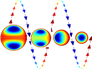
After having considered the mass evaporation rate of the droplet, we will now look into the liquid phase to understand the spatio-temporal temperature and concentration distributions of the evaporating droplet. In this work, any possible deformation in droplet shape due to aerodynamic forces has been neglected. This can be justified by assessing the gas-phase Weber number,  $We=2\rho _g(|U_p-U_g|)^2r_s/\sigma$, which is significantly less than 1 for the conditions of this study. The liquid phase of a spherical droplet translating in the gas phase experiences convective vortical motion due to relative velocity and, thus, shear stress at the liquid–gas interface. Abramzon & Sirignano (Reference Abramzon and Sirignano1989) showed, for such droplets, that the internal flow structure can be modelled as the well-known two-dimensional Hill's spherical vortex (Lamb Reference Lamb1993). The explicit solution for a Hill's spherical vortex renders expressions for the radial and angular velocities in the spherical coordinate system $(r,\theta )$ in the liquid phase as follows:
 \begin{equation} V_r={-}U_s\left(1-\frac{r^2}{r_s^2}\right)\cos\theta, \end{equation}
and
 \begin{equation} V_{\theta}=U_s\left(1-2\frac{r^2}{r_s^2}\right)\sin\theta. \end{equation}
Here  $U_s=(1/32)(U_g-U_p)(\mu _g/\mu _l)Re_pC_F$ is the liquid velocity at the vapour–liquid interface and is calculated by the continuity of the shear stress across the interface; $\mu _l$ is the liquid-phase dynamic viscosity; and $C_F$ is the skin friction coefficient for an evaporating sphere calculated using the correlation given by Renksizbulut & Yuen (Reference Renksizbulut and Yuen1983) as
 \begin{equation} C_F=\frac{12.69Re_p^{{-}2/3}}{1+B_M}. \end{equation}
It is to be noted that thermal and concentration gradients across the droplet interface can induce Marangoni stress, which can be important for modelling the evaporation of multicomponent droplets (Niazmand et al. Reference Niazmand, Shaw, Dwyer and Aharon1994; Dwyer et al. Reference Dwyer, Aharon, Shaw and Niamand1996; Dwyer, Shaw & Niazmand Reference Dwyer, Shaw and Niazmand1998). However, for the present study, the gradients are small, and, as such, the Marangoni flow velocity is expected to be smaller than the shear-driven flow ( $U_s$) at the droplet surface. A detailed comparison is shown in the supplementary material.
The non-dimensional conservation equations of energy and mass fraction in the liquid phase are given by (Ozturk & Cetegen Reference Ozturk and Cetegen2004)
 \begin{align} &\overline{r_s^2}\frac{\partial\bar{T}}{\partial\bar{t}} +(0.5Pe_l\overline{V_r}\overline{r_s}-\beta\eta)\frac{\partial\bar{T}}{\partial\eta} +0.5Pe_l\frac{\overline{V_{\theta}}\overline{r_s}} {\eta}\frac{\partial\bar{T}}{\partial\theta} \nonumber\\ &\quad=\frac{1}{\eta^2}\frac{\partial}{\partial\eta} \left(\eta^2\frac{\partial\bar{T}}{\partial\eta}\right) +\frac{1}{\eta^2\sin\theta}\frac{\partial}{\partial\theta} \left(\sin\theta\frac{\partial\bar{T}}{\partial\theta} \right) \end{align}
and
 \begin{align} &Le_l\overline{r_s^2}\frac{\partial\overline{Y_N}}{\partial\bar{t}}+(0.5Pe_l Le_l\overline{V_r}\overline{r_s}-Le_l\beta\eta) \frac{\partial\overline{Y_N}}{\partial\eta}+0.5Pe_l Le_l\frac{\overline{V_{\theta}}\overline{r_s}}{\eta} \frac{\partial\overline{Y_N}}{\partial\theta}\nonumber\\ &\quad=\frac{1}{\eta^2}\frac{\partial}{\partial\eta} \left(\eta^2\frac{\partial\overline{Y_N}}{\partial\eta}\right) +\frac{1}{\eta^2\sin\theta}\frac{\partial}{\partial\theta} \left(\sin\theta\frac{\partial\overline{Y_N}}{\partial\theta}\right), \end{align}
respectively. Equations (2.20) and (2.21) are solved using the initial and boundary conditions,
 \begin{equation} \left. \begin{aligned} & \bar{t}=0\rightarrow \bar{T}=0,\\ & \eta=1, \quad \begin{cases} \dfrac{\partial\bar{T}}{\partial\theta}=0,\\ \displaystyle\int_0^{\rm \pi} \dfrac{\partial\bar{T}}{\partial\eta}\sin\theta\, {\rm d}\theta =\dfrac{\dot{Q}_l}{2{\rm \pi} r_s k_l T_0}, \end{cases}\\ & \theta=0, \quad {\rm \pi}\rightarrow \frac{\partial\bar{T}}{\partial\theta}=0, \end{aligned} \right\} \end{equation}
and
 \begin{equation} \left. \begin{aligned} & \bar{t}=0\rightarrow \overline{Y_N}=0,\\ & \eta=1,\quad \begin{cases} \dfrac{\partial\overline{Y_N}}{\partial\theta}=0,\\ \displaystyle\int_0^{\rm \pi} \dfrac{\partial\overline{Y_N}}{\partial\eta}\sin\theta \,{\rm d}\theta =\dfrac{\dot m}{2{\rm \pi}\rho_l r_s D_{v,za} Y_{N,0},}, \end{cases}\\ & \theta=0,\quad {\rm \pi}\rightarrow \frac{\partial\overline{Y_N}}{\partial\theta}=0, \end{aligned} \right\} \end{equation}
respectively. Here,  $\overline {r_s}=r_s/r_0$ is the non-dimensional droplet radius; $\eta =r/r_s$ is the non-dimensional radial coordinate; $\overline {V_r}=V_r/U_s$ and $\overline {V_{\theta }}=V_{\theta }/U_s$ are the non-dimensional velocities (radial and angular, respectively); $\bar {T}=(T-T_0)/T_0$ is the non-dimensional temperature; $\bar {t}=\alpha _lt/r_0^2$ is the non-dimensional time; $\beta =0.5\partial \overline {r_s}/\partial \bar {t}$ is the non-dimensional parameter proportional to the droplet's surface regression rate as it vaporizes; $\alpha _l$ is the thermal diffusivity of the liquid phase; $\dot {Q}_l$ is the heat transferred into the liquid; $\overline {Y_N}=(Y_N-Y_{N,0})/Y_{N,0}$ is the normalized mass fraction of the solute; $k_l$ is the thermal conductivity of the liquid phase; $D_{v,za}$ is the mass diffusivity of solute in solvent; and $Pe_l\ (=r_s|U_g-U_p|/\alpha _l)$ and $Le_l\ (=D_{v,za}/\alpha _l)$ are the Péclet number and Lewis number of the liquid phase, respectively.
The above set of equations of the model show that the liquid-phase transport affects the temperature and concentration at the droplet surface. This, in turn, affects the evaporation rate and, thus, the droplet size. The droplet size, on the other hand, determines the drag forces, which control the velocity and acceleration of the droplet. The instantaneous droplet velocity affects the heat and mass transfer in the gas phase and, hence, the evaporation rate. Both gas-phase and liquid-phase properties play critical roles in determining the relative effects of these complex coupled processes. In summary, the evaporation of an isolated droplet moving in the gas phase, indeed, involves complex coupled processes.
All the above equations (2.1)–(2.23) are solved numerically, for both external vapour and internal liquid regions. However, in order to solve the liquid phase, the boundary conditions presented in (2.22) and (2.23) need values from the vapour-phase solution. Therefore, a numerical integration method using a forward marching scheme is implemented to solve (2.1). Moreover, the instantaneous droplet radius (2.8) is also computed by a forward marching scheme using the mass flux  $\dot m$ generated from (2.9). Furthermore, $\dot {Q}_l$ is solved using Spalding heat transfer number $B_T$, and both $\dot {Q}_l$ and $\dot m$ are employed in the boundary conditions (2.22) and (2.23).
After deriving the boundary conditions from the vapour-phase solution, the energy (2.20) and species (2.22) conservation equations of the droplet's liquid phase along with the boundary conditions (2.22) and (2.23) are numerically computed by a fully implicit iterative finite difference scheme called standard second-order Peaceman–Rachford alternating direction implicit method (Peaceman & Rachford Reference Peaceman and Rachford1955). The details of the numerical algorithm used in this work can be found in Majee et al. (Reference Majee, Saha, Chaudhuri, Chakravortty and Basu2021). The consideration of an implicit scheme guarantees an unconditionally stable method. It is to be noted that the liquid phase inside the droplet was solved using a polar ( $r$–
$r$– $\theta$) coordinate system, where both dimensions were discretized using an equal number (20 for this study) of grid points, leading to $\Delta \eta =0.05$ and $\Delta \theta =0.157$ being taken for the entire simulation process. We have performed a grid convergence study using various grid sizes (see the supplementary material for details). We used a time step of $\Delta t=0.0001$, which is short enough to capture the transport processes. The property values used for this study can be found in the supplementary material.
3. Results and discussion
As mentioned before, the primary goal of this work is to assess the response in droplet evaporation rate under various degrees of oscillations in gas-phase velocity, given by (2.7). This will be attained by modulating the frequency ( $f$) and amplitude ( $a$) of the oscillation. As for the binary droplet, we assumed that it contains 1 % (w/w) of NaCl (solute) dissolved in water (solvent). Here, we note that a wide range of solute–solvent combinations can be selected for such a study. However, we chose the NaCl solution because (1) it is easily available for experimental validation and (2) it closely resembles surrogate respiratory fluids (Vejerano & Marr Reference Vejerano and Marr2018; Basu et al. Reference Basu, Kabi, Chaudhuri and Saha2020). Similarly, a wide range of ambient (temperature and humidity) conditions could be selected for this study. However, we used conditions that closely resemble that of our ambient air ( $T_{amb}=301~\textrm {K}$ and $RH_{amb}=48\,\%$).
3.1. Model validation
To validate the model, we first compare the numerical result with a simple experimental set-up. The experiments were conducted by measuring the evaporation rate of an isolated acoustically levitated droplet with 1 % (w/w) NaCl aqueous solution in  $301\pm 0.2~\textrm {K}$ ambient temperature and $48\,\%\pm 1\,\%$ relative humidity. For these experiments, the droplets were at the same temperature as the surrounding air ( $301~\textrm {K}$). Air vortex rings were generated with amplitude $a=1.9~\textrm {m}~\textrm {s}^{-1}$ and frequency $f=5~\textrm {Hz}$ and are made to interact with the levitated droplet of initial diameter $D_0=1.8~\textrm {mm}$. The mean flow in the experimental set-up is $0.3~\textrm {m}~\textrm {s}^{-1}$. The details of these experiments are provided in Sharma, Singh & Basu (Reference Sharma, Singh and Basu2021) and Sharma et al. (Reference Sharma, Jain, Saha and Basu2022). Experimentally, we can only measure the droplet diameter as a function of time, which has been compared with the model for two cases, i.e. with the vortex (unsteady case) and without the vortex (steady case). Since the precipitation kinetics was not included in the current approach, the comparison was performed until the maximum local concentration of the solution (NaCl in this case) reached the critical value $Y_{N,S}$ ( $=0.393$ for NaCl). Nevertheless, figure 1, which shows the $(D/D_0)^2$ versus $t$ comparisons between the experiments and the model, confirms that they show reasonably good agreement. Similar agreements were also observed for other amplitude and frequency cases. Thus, we are confident that the model can capture the effects of unsteady gas flow on the evaporation dynamics of an isolated droplet.

Figure 1. Model validation: comparison of diameter regression,  $(D/D_0)^2$, between experimental (levitated droplet) and model data. ‘Steady’ represents experiments with no vortical flow. ‘Vortex’ represents experiments with vortical flow over a levitated droplet. In experiments, the initial droplet diameter is $D_0=1.8~\textrm {mm}$.
3.2. Evaporation dynamics of the droplet
In the remainder of this article, we discuss the results from the model to illustrate the effect of a broad range of periodic oscillations in the gas-phase velocity on the evaporation dynamics of an isolated droplet. As mentioned before, we will keep the ambient conditions fixed with  $RH_{amb}=48\,\%$ and $T_{amb}=301~\textrm {K}$. The initial droplet temperature was taken as $303~\textrm {K}$, which closely resembles the temperature of respiratory droplets ejected during respiratory events (Carpagnano et al. Reference Carpagnano, Foschino-Barbaro, Crocetta, Lacedonia, Saliani, Zoppo and Barnes2017). To avoid a negative gas-phase velocity, the mean velocity of the gas phase was kept equal to the amplitude of the gas-phase oscillation, i.e. $U_{g,0}=a$.
We now present the diameter regression rate for various degrees of flow oscillation for two different droplet sizes. First, we compare the evaporation dynamics of a  $100~\mathrm {\mu }\textrm {m}$ droplet under various frequencies of oscillation at amplitude ( $a$) of 0.1 m s $^{-1}$ (figure 2a) and 1 m s $^{-1}$ (figure 2b). We observed that, for a lower amplitude of perturbation ( $a=0.1~\textrm {m}~\textrm {s}^{-1}$), the deviation in $(D/D_0)^{2}$ with the steady ( $a=0$) case is minimal compared with the high-amplitude ( $a=1~\textrm {m}~\textrm {s}^{-1}$) case. Although, with an increase in frequency, the evaporation time becomes shorter for the low-amplitude oscillations, the difference between various frequencies is minimal (figure 2a). For larger amplitude, however, we see almost 30 % decrease in time for $(D/D_0)^2$ to reach 0.1 (approximately when precipitation is triggered) for $f=30~\textrm {Hz}$ compared with $f=1~\textrm {Hz}$, as shown in figure 2(b).

Figure 2. Normalized droplet diameter as a function of time for various combinations of initial droplet diameters ( $D_0$), amplitude ( $a$) and frequency ( $f$) of gas-phase oscillation: (a) $D_0=100~\mathrm {\mu }\textrm {m}$ and $a=0.1~\textrm {m}~\textrm {s}^{-1}$; (b) $D_0=100~\mathrm {\mu }\textrm {m}$ and $a=1~\textrm {m}~\textrm {s}^{-1}$; (c) $D_0=594\ \mathrm {\mu }\textrm {m}$ and $a=0.1~\textrm {m}~\textrm {s}^{-1}$; and (d) $D_0=594~\mathrm {\mu }\textrm {m}$ and $a=1~\textrm {m}~\textrm {s}^{-1}$. Legends: ‘steady’, no gas-phaseoscillation; $D_0$, initial droplet diameter in $\mathrm {\mu }\textrm {m}$; $f$, frequency in $\textrm {Hz}$; and $a$, amplitude in $\textrm {m}~\textrm {s}^{-1}$.
Next, we compare the same amplitude and frequency of oscillations for a larger droplet ( $D_0=594~\mathrm {\mu }\textrm {m}$) in figure 2(c,d). We observe similar behaviour, in that an increase in amplitude and frequency increases the evaporation rate. However, for both amplitudes, we do not observe significant changes in evaporation rate across various frequencies from 1–30 Hz. Nevertheless, the evaporation is much faster with oscillations (non-zero $a$) than the steady ( $a=0$) case (14 % for $a=0.1~\textrm {m}~\textrm {s}^{-1}$ and 40 % for $a=1~\textrm {m}~\textrm {s}^{-1}$). The cause of such varying influence of oscillation on the evaporation rate for different droplet sizes and oscillation parameters will be discussed later in the context of the modified Reynolds number.
3.3. Velocity of gas phase and droplet motion
The comparisons in the previous subsection show that the effect of oscillation in gas-phase velocity on the evaporation rate is nonlinear. We note that the evaporation rate of the droplet strongly depends on the Nusselt and Sherwood numbers ((2.9) and (2.10)), which depend on the droplet Reynolds numbers ((2.11)–(2.16)), and hence on the relative velocity between the droplet and the surrounding gas phase (2.5). Thus, we investigate the effects of oscillation in gas-phase velocity on the bulk velocity of the droplet. In figures 3 and 4, we compare the instantaneous gas-phase velocity ( $U_g$) and droplet velocity ( $U_p$) during the evaporation process for two different droplet diameters and frequencies of oscillation. In both cases, the mean velocity ( $U_{g,0}$) and amplitude ( $a$) of the gas-phase flow were maintained to be 1 m s $^{-1}$.

Figure 3. The instantaneous velocities of the gas phase ( $U_g$) and the droplet ( $U_p$) as functions of time for initial droplet size $D_0=100~\mathrm {\mu } \textrm {m}$. The gas-phase oscillation has amplitude $a=1~\textrm {m}~\textrm {s}^{-1}$ and frequency of $f =5~\textrm {Hz}$.

Figure 4. The instantaneous velocities of the gas phase ( $U_g$) and the droplet ( $U_p$) as functions of time for initial droplet size $D_0=594~\mathrm {\mu }\textrm {m}$. The gas-phase oscillation has amplitude $a=1~\textrm {m}~\textrm {s}^{-1}$ and frequency of $f =30~\textrm {Hz}$.
For smaller droplets ( $D_0=100~\mathrm {\mu }\textrm {m}$) and lower-frequency oscillation ( $f=5~\textrm {Hz}$), we observe the droplet velocity ( $U_p$) to exhibit a periodic behaviour as well (figure 3). Figure 3(b), which shows an expanded view of the initial 1 s of the droplet lifetime, confirms that, initially, the amplitude of the induced oscillation in the $U_p$ has an amplitude slightly smaller than that of the gas phase, and that there exists a phase lag. However, at a later stage (figure 3c), the difference between the two velocities, gas phase ( $U_g$) and droplet ( $U_p$), becomes negligible, and their oscillations become almost identical in both phase and amplitude.
On the other hand, for a larger droplet ( $D_0=594~\mathrm {\mu }\textrm {m}$) and higher frequency ( $f=30~\textrm {Hz}$) of oscillation, we observe different dynamics (figure 4). In particular, the oscillation in droplet velocity takes longer to attain that of the gas phase. Furthermore, we observe much slower growth in the amplitude of oscillation in $U_p$, which never grows beyond 10 % before precipitation is triggered ( ${\sim }$265 s). We also observe a consistent phase lag between the oscillation in $U_g$ and $U_p$.
3.4. Theoretical scaling analysis
In this section, we present a time-scale analysis to understand the observed dynamics of induced oscillation in the droplet velocity ( $U_p$). For gas-phase oscillation of $U_g=U_{g,0}+a\sin (2{\rm \pi} f t)$, we can evaluate the induced oscillation in droplet velocity by integrating the equation for drag (2.6) with the initial condition of $U_p=0$ at $t=0$ (initial droplet velocity is zero). We recall the definitions of the drag coefficient ( ${C_D=24/Re_p}$) and Reynolds number ( ${Re_p=2\rho _g| U_g-U_p | r_s/\mu _g}$). We can also define ${\tau =({\rho _l r_s^2})/\mu _g}$ as the response time for a spherical droplet in a viscous flow, and ${t_g=1/f}$ as the characteristic time scale for gas-phase oscillation. The droplet response in an unsteady flow is characterized by Stokes number ${St=\tau /t_g}$ (Crowe, Sommerfeld & Tsuji Reference Crowe, Sommerfeld and Tsuji1998), which represents the ratio of the characteristic time scale for droplet response ( $\tau$) to that of the external flow ( ${t_g}$). In the context of our study with oscillatory gas-phase velocity, the Stokes number can be written as ${St=\tau f}$.
Now substituting these definitions in (2.6), we get a non-dimensional drag equation:
 \begin{equation} \frac{{\rm d}((U_p-U_{g,0})/a)}{{\rm d}(t/t_g)} ={-}\frac{9}{2St}\left(\frac{U_p-U_{g,0}}{a}\right) +\frac{9}{2St}\sin\left(2{\rm \pi}\frac{t}{t_g}\right). \end{equation}
In the equation above, we notice that the non-dimensional droplet velocity,  ${(U_p-U_{g,0})/a}$, depends on ${St}$, which includes the effect of instantaneous droplet radius and ${t/t_g}$, a non-dimensional time.
For simplicity, we restrict the analysis to a non-evaporating spherical droplet, and, hence, the droplet radius ( $r_s$) and the Stokes number ( $St$) are assumed to be constant. Later, we will discuss the effect of this assumption on the obtained results. With this assumption, we can integrate (3.1) to find an explicit form of the non-dimensional droplet velocity:
 \begin{equation} \frac{U_p-U_{g,0}}{a}=\frac{\sin({2{\rm \pi}} (t/t_g)-\phi)} {\sqrt{1+(16{\rm \pi}^2St^2/{81})}} + \left( -\frac{U_{g,0}}{a} + \frac{4{\rm \pi} St/{9}}{({1+(16{\rm \pi}^2St^2/{81})})} \right) {\rm e}^{-{9t}/{(2t_gSt)}}, \end{equation}
where  $\phi =\tan ^{-1} ( 4{\rm \pi} St/9 )$.
Equation (3.2) depicts the response in velocity of a non-evaporating spherical droplet when the surrounding gas phase has an oscillatory perturbation. The first term on the right-hand side represents the induced oscillation in droplet velocity. We notice that the frequency of the induced oscillation in droplet velocity is the same as the gas-phase perturbation (  $f$ or $1/t_g$), while the non-dimensionalized amplitude of the induced oscillation is $A_{osc}=1/\sqrt {1+(16{\rm \pi} ^2St^2/{81})}$. The induced oscillation in the droplet velocity lags the oscillation in gas-phase velocity by a phase angle, $\phi$. The second term on right-hand side shows the effect of viscous drag, which exponentially reduces the difference between the mean velocities of the droplet and the gas phase. It is worth noting that, for a steady gas-phase flow (i.e. $a=0$), the oscillatory term vanishes, and (3.2) reduces to the classical exponential relation for a non-evaporating droplet (or spherical object) in a gaseous flow field, $U_{p,0}=U_{g,0}(1- \textrm {e}^{-9t/(2t_gSt)})$.
To graphically illustrate the droplet response expressed in (3.2), we present the contour plot of the normalized droplet velocity,  $(U_p-U_{p,0})/a$, for a large range of $St$ ( $Y$-axis) and non-dimensional time $t/t_g$ ( $X$-axis) in figure 5(a). Since $U_{p,0}$ is the droplet velocity in a steady gas-phase flow, $(U_p-U_{p,0})/a$ measures the modification in droplet velocity due to the unsteady oscillations in the gas phase. Furthermore, we also plotted the amplitude ( $A_{osc}$) and phase ( $\phi$) of the induced oscillation in droplet velocity as a function of $St$ in figure 5(b).

Figure 5. (a) Contour plot of non-dimensional change in droplet velocity,  $(U_p-U_{p,0})/a$, with Stokes number ( $St$) and non-dimensional time ( $t/t_g$), where $t_g$ is the gas-phase perturbation time. History of Stokes number ( $St$) for different initial diameters and frequencies is plotted on the contour map. Legend: $D_0$, initial diameter in $\mathrm {\mu }\textrm {m}$; and $f$, frequency of gas-phase oscillation in $~\textrm {Hz}$. For all five cases, the amplitude of the gas-phase oscillation is $a=1~\textrm {m}~\textrm {s}^{-1}$. (b) Variation in amplitude ( $A_{osc}=1/\sqrt {1+(16{\rm \pi} ^2St^2/{81})}$) and phase lag ( $\phi =\tan ^{-1} (4{\rm \pi} St/9 )$) of the induced oscillation in non-dimensional droplet velocity, $({U_p-U_{g,0}})/{a}$, as a function of Stokes number ( $St$).
From the contour plot (figure 5a), we can see that, for a small  $St$ ( ${\ll } 1$), the droplet velocity, $(U_p-U_{p,0})/a$, exhibits a periodic behaviour with time, expressed by the colour bands in the horizontal direction. The periodicity in the colour band appears to be non-uniform due to the log scale used on the $X$-axis. A dominant periodic behaviour at small $St$ is expected, as the second term on the right-hand side of (3.2) is small. The amplitude of the induced oscillation for this case ( $St\ll 1$) is also high and close to that of the gas-phase perturbation ( $A_{osc}\approx 1$), as seen in figure 5(b). As $St$ increases and approaches 1, the periodic pattern still exists, but the difference between the maximum and minimum instantaneous velocity (colour variation in figure 5a) becomes weaker due to the reduced amplitude of the induced oscillation ( $A_{osc}$ in figure 5b). We also notice that the maximum velocity zones (bright yellow zones) in the contour plot shift towards the right. This is the outcome of increased phase lag $\phi$ between droplet and gas-phase velocities with increasing $St$ (figure 5b). For very large $St$ ( ${\gg } 1$), the denominator of the first term on the right-hand side of (3.2) becomes significantly greater than unity. As such, the amplitude of the oscillation becomes minimal ( $A_{osc}$ in figure 5b). This is why the colour variation in the horizontal direction (as a function of time) diminishes in the top half of the contour plot ( $St\gg 1$ in figure 5a).
The above analyses can also be performed by considering the variation in droplet radius due to evaporation. However, such an approach, shown in Appendix A, does not lead to a closed-form expression for the droplet velocity. Furthermore, it can be shown (see Appendix A) that the difference in the change in droplet velocity due to oscillation,  $(U_p-U_{p,0})/a$, evaluated using the two approaches (with and without the assumption of constant droplet radius) is relatively insignificant. Hence, we used the constant droplet assumption for the rest of the study.
Now, to illustrate the range of  $St$ experienced by the evaporating droplets, we plotted the instantaneous $St$ obtained from the simulation of various cases on the theoretical contour plot in figure 5(a). Since the droplet diameter and, hence, $\tau$ decrease due to evaporation, the $St$ value shows a downward decreasing trend with non-dimensional time ( $t/t_g$). We observe that the cases with a small initial diameter ( $D_0=100~\mathrm {\mu }\textrm {m}$) and lower-frequency oscillations ( $f=1$ and 5 Hz) experience low $St$ and, hence, large-amplitude oscillations in velocity (figure 5a). This effect is also observed in figure 3, where we showed that, for $D_0=100~\mathrm {\mu }\textrm {m}$ and $f=5~\textrm {Hz}$, the amplitude of oscillation in droplet velocity quickly attains that of the gas-phase velocity. As the frequency of oscillation in gas-phase velocity ( $f$) increases, $St$ increases, reducing the amplitude of induced oscillation in droplet velocity ( $f = 1$, 5 and 30 Hz in figure 5a). For larger droplets ( $D_0=594~\mathrm {\mu }\textrm {m}$), the $St$ value becomes significantly greater than unity, and hence they do not exhibit significant induced oscillations in velocity. For $D_0=594~\mathrm {\mu }\textrm {m}$ and $f=30~\textrm {Hz}$, we observe a weak response, and hence the amplitude becomes inconsequential to the frequency change (figure 4).
Next, we will assess the effect of oscillation in gas-phase flow on  $Re_p$, which, in turn, affects the evaporation rate. Since the external conditions are kept constant in our simulations, the changes in diameter reduction rate observed in figure 2(a–d) are through the Sherwood ( $Sh^*$) and Nusselt ( $Nu^*$) numbers in (2.9) and (2.10), respectively. Equations (2.11)–(2.16) subsequently show that an increase in $Re_p$ increases both $Sh^*$ and $Nu^*$, and hence the evaporation rate. Since the Reynolds number ( $Re_p$) is defined based on the relative velocity between the gas phase and the droplet, one can evaluate the induced $Re_p$ due to gas-phase velocity oscillation by substituting $U_p$ (3.2) and $U_g$ (2.7) into (2.5). Similarly, it is also possible to evaluate the Reynolds number of the droplet without the gas-phase oscillation ( $a=0$) as $Re_{p,0}=2\rho _g| U_{g,0}-U_{p,0} | r_s/\mu _g$. Clearly, higher (or lower) values of the ratio $Re_p / Re_{p,0}$ signify stronger (or weaker) effects of gas-phase oscillation on the evaporation rate compared with the steady condition ( $a=0$).
Figure 6(a) shows the contours of this ratio ( $Re_p/Re_{p,0}$) for a range of $St$ and normalized time, $t/t_g$. Based on the colour, the map can be divided (almost diagonally) into two parts separated by the dotted line, $St_{crit}$. The top-left half, where the instantaneous values of $Re_p/Re_{p,0}$ are close to unity ( $10^0$ in the plot), represents a zone where the relative effects of gas-phase oscillation on $Re$ with respect to $Re_{p,0}$ is small, and hence can be characterized as a ‘zone of silence’. The change in droplet velocity ( $U_p-U_{p,0}\approx 0$) due to gas-phase oscillation is, indeed, weak, as observed in figure 5(a). Furthermore, under steady flow conditions, the relative velocity between the droplet and the gas phase (hence, $Re_{p,0}$) is high.

Figure 6. (a) Contour plot for  $Re_p/Re_{p,0}$ with Stokes number ( $St$) and non-dimensional time ( $t/t_g$), where $t_g$ is the gas-phase perturbation time. History of Stokes number ( $St$) for different initial diameters and frequencies is plotted on the contour map. Legend: $D_0$, initial diameter in $\mathrm {\mu }\textrm {m}$; and $f$, frequency of gas-phase oscillation in $\textrm{Hz}$. For all five cases, the amplitude of the gas-phase oscillation is $a=1~\textrm {m}~\textrm {s}^{-1}$. (b) Time history of changes in droplet Reynolds number due to gas-phase oscillation ( $\Delta Re_p= Re_p - Re_{p,0}$) for amplitude $a=1~\textrm {m}~\textrm {s}^{-1}$, frequencies ( $f=1$, 10 and 30 Hz). The initial droplet diameter ( $D_0$) is $594~\mathrm {\mu }\textrm {m}$. (c) The average changes in droplet Reynolds number due to gas-phase oscillation ( $\overline {\Delta Re_p}$, averaged $\Delta Re_p$) as a function of frequency $f$ of gas-phase oscillation for different amplitudes ( $a$ in $\textrm {m}~\textrm {s}^{-1}$) and initial droplet diameters ( $D_0$ in $\mathrm {\mu }\textrm {m}$).
On the other hand, the bottom-right half of figure 6(a) represents a zone where  $Re_p/Re_{p,0}$ has a very high value, and hence can be characterized as a ‘zone of influence’. In this regime, droplet velocity ( $U_p$) displays strong oscillatory behaviour, as shown in figure 5(a). Furthermore, under steady gas-phase flow ( $a=0$), the differences between the droplet velocity become small (and hence $Re_{p,0}\rightarrow 0$). Consequently, for a given $t/t_g$, the transition between the ‘zone of silence’ and the ‘zone of influence’ can be marked by a critical Stokes number ( $St_{crit}$) for which $U_{p,0} \rightarrow U_{g,0}$. In figure 6(a), a representative transitional boundary is drawn by setting $(U_{p,0}-U_{g,0})/U_{g,0}=10^{-5}$. The $St$ history from a few simulated conditions are superimposed on the contour plot. We observe that, initially, the droplet starts from the ‘zone of silence’, but transitions into the ‘zone of influence’ (figure 6) as time progresses and the droplet becomes smaller due to evaporation.
While  $Re_p/Re_{p,0}$ depicts the relative change in $Re_p$ due to oscillation in the gas phase, it is to be recognized that $Re_{p,0} \approx 0$ in the ‘zone of influence’, and, as such, the ratio becomes large, even for a small $Re_p$. To circumvent this bias and to assess the true effect on the evaporation rate, one should evaluate their differences, i.e. $\Delta Re_p = Re_p-Re_{p,0}$. In figure 6(b), we plotted $\Delta Re_p$ as a function of time for a given initial droplet size ( $D_0 =594~\mathrm {\mu }\textrm {m}$) and amplitude ( $a=1~\textrm {m}~\textrm {s}^{-1}$), but for three different frequencies ( $f=1$, 10 and 30 Hz) of gas-phase oscillation. The plot displays large-amplitude oscillations in $\Delta Re_p$ at the initial stage. However, the amplitude decays with time and becomes almost constant in the later stage of the droplet lifetime (see inset of figure 6b). This behaviour, indeed, corroborates the dynamics of droplet velocity, $U_p$, described before.
To estimate an overall change in  $Re_p$ due to oscillation in gas-phase flow, we evaluated the mean of $\Delta Re_p$ (denoted by $\overline {\Delta Re_p}$) for four combinations of amplitude ( $a$) and initial droplet diameter ( $D_0$) and plotted them as a function of frequency ( $f$) of gas-phase oscillation in figure 6(c). For smaller droplets ( $D_0=100~\mathrm {\mu }\textrm {m}$) and lower amplitude ( $a=0.1~\textrm {m}~\textrm {s}^{-1}$) of oscillation, the $\overline {\Delta Re_p}$ value is small ( $\sim 10^{-1}$), which explains why we did not observe significant changes in evaporation rate among various frequencies as shown in figure 2(a). On the other hand, for larger amplitude ( $a=1~\textrm {m}~\textrm {s}^{-1}$), $\overline {\Delta Re_p}$ is relatively higher ( $\sim 1$), and increases with $f$. Thus, we observed a faster evaporation rate with oscillations, which increases with frequency (figure 2b). Figure 6(c) also confirms that $\overline {\Delta Re_p}$ for larger droplets ( $D_0=594~\mathrm {\mu }\textrm {m}$) is higher and remains almost constant for all $f$, irrespective of the amplitude ( $a=0.1$ and $1$ m s $^{-1}$). This explains the observed faster evaporation under unsteady gas-phase flow but the insignificant difference between various frequencies (figure 2c,d) for the larger droplets.
3.5. Temperature and concentration distributions in the liquid phase
Since our model includes transport equations for the liquid phase, we can compare the temperature and concentration distributions inside the droplet to illustrate the effect of unsteadiness in gas-phase velocities on the liquid-phase transport. Figures 7 (temperature) and 8 (mass fraction of solute) display the evolutions of the internal dynamics for three instances on the lifetime of a  $D_0=100~\mathrm {\mu }\textrm {m}$ droplet and compare them for three different degrees of oscillations in the gas phase. Similar contour plots for $D_0=594~\mathrm {\mu }\textrm {m}$ are shown in figures 9 (temperature) and 10 (mass fraction of solute). Here, we recall that the ambient condition for the simulation was $T_{amb}=301~\textrm {K}$ and $RH_{amb}=48\,\%$, while the initial droplet temperature was set at $303~\textrm {K}$ and initial solute (NaCl) concentration dissolved in water was $Y_{N,0}=1\,\%$.

Figure 7. Temperature distribution in the liquid phase at different time steps for  $D_0=100~\mathrm {\mu }\textrm {m}$ with initial droplet temperature, $T_0 = 303~\textrm {K}$. The ambient condition is $T_{amb}=301~\textrm {K}$ and $RH_{amb}=48\,\%$. The gas-phase perturbation: (a) amplitude, $a = 0.1~\textrm {m}~\textrm {s}^{-1}$, and frequency, $f= 5~\textrm {Hz}$; (b) $a= 1~\textrm {m}~\textrm {s}^{-1}$ and $f=5~\textrm {Hz}$; and (c) $a=1~\textrm {m}~\textrm {s}^{-1}$ and $f=30~\textrm {Hz}$.

Figure 8. Solute concentration distribution in the liquid phase at different time steps for  $D_0=100~\mathrm {\mu }\textrm {m}$ with initial droplet temperature, $T_0 = 303~\textrm {K}$. The ambient condition is $T_{amb}=301~\textrm {K}$ and $RH_{amb}=48\,\%$. The gas-phase perturbation: (a) amplitude, $a = 0.1~\textrm {m}~\textrm {s}^{-1}$, and frequency, $f= 5~\textrm {Hz}$: (b) $a= 1~\textrm {m}~\textrm {s}^{-1}$ and $f=5~\textrm {Hz}$: and (c) $a= 1~\textrm {m}~\textrm {s}^{-1}$ and $f= 30~\textrm {Hz}$.

Figure 9. Temperature distribution in the liquid phase at different time steps for  $D_0=594~\mathrm {\mu }\textrm {m}$ with initial droplet temperature, $T_0 = 303~\textrm {K}$. The ambient condition is $T_{amb}=301~\textrm {K}$ and $RH_{amb}=48\,\%$. The gas-phase perturbation: (a) amplitude, $a = 0.1~\textrm {m}~\textrm {s}^{-1}$, and frequency, $f = 5~\textrm {Hz}$: (b) $a=1~\textrm {m}~\textrm {s}^{-1}$ and $f=5~\textrm {Hz}$; and (c) $a = 1~\textrm {m}~\textrm {s}^{-1}$ and $f = 30~\textrm {Hz}$.

Figure 10. Solute concentration distribution in the liquid phase at different time steps for  $D_0=594~\mathrm {\mu }\textrm {m}$ with initial droplet temperature, $T_0 = 303~\textrm {K}$. The ambient condition is $T_{amb}=301~\textrm {K}$ and $RH_{amb}=48\,\%$. The gas-phase perturbation: (a) amplitude, $a = 0.1~\textrm {m}~\textrm {s}^{-1}$, and frequency, $f = 5~\textrm {Hz}$; (b) $a = 1~\textrm {m}~\textrm {s}^{-1}$ and $f=5~\textrm {Hz}$; and (c) $a= 1~\textrm {m}~\textrm {s}^{-1}$ and $f=30~\textrm {Hz}$.
Figures 7 and 9 depict that, in the early stage of evaporation, the temperature distribution displays a symmetric concentric profile. This is the hallmark of stronger diffusional transport than advective transport of thermal energy (Sirignano Reference Sirignano1983; Abramzon & Sirignano Reference Abramzon and Sirignano1989; Saha et al. Reference Saha, Singh, Seal and Basu2009b) caused by large thermal diffusivity in the liquid phase. The enhanced thermal transport and smaller initial temperature difference between the gas phase and liquid phase enable the droplet to reach the wet-bulb temperature and attain homogeneity in a short duration, as seen in both figures 7 and 9. Owing to the dominant diffusive transport in the liquid phase, the effects of amplitude and frequency of the gas-phase oscillation on the temperature profiles are not significant.
Figures 8 and 10 show the concentration distribution of solute in the liquid phase for two different droplet sizes. We notice that the lower amplitude of gas-phase oscillation ( $a=0.1~\textrm {m}~\textrm {s}^{-1}$) leads to a diffusion-dominated concentric distribution even in the early stage of droplet lifetime (figures 8a and 10a). On the other hand, for high-amplitude oscillations ( $a=1~\textrm {m}~\textrm {s}^{-1}$), a recirculation pattern was formed inside the droplet, which resembles the internal flow pattern (Hill's spherical vortex) (figures 8b,c and 10b,c). This indicates strong advective transport. The relative strength between advective and diffusive mass transport can be expressed by the Péclet number, $Pe_l=Re_l Sc$, where $Sc$ is the Schmidt number (roughly constant). The liquid-phase Reynolds number, $Re_l$, is defined based on the (liquid-phase) velocity at the vapour–liquid interface ( $U_s$) driven by gas-phase flow or $Re_p$ ((2.17) and (2.18)). As shown in figure 5, an increase in the amplitude of oscillation increases $Re_p$, and hence $Pe_l$. This is why we observe stronger advective transport for the higher amplitude of gas-phase oscillation (figures 8 and 10) in the early stage of evaporation. As the droplet evaporates, $Re_p$ decreases. As such, both $Pe_l$ and the advective transport in the liquid phase become weaker, resulting in more concentric iso-concentration lines for $D_0=100~\mathrm {\mu }\textrm {m}$ droplets (figure 8b,c). However, for $D_0=594~\mathrm {\mu }\textrm {m}$, $Re_l$ and $Pe_l$ remain comparatively higher throughout the droplet lifetime due to larger droplet diameters. Thus, convective transport remains strong, as reflected in vortical isocontours in figure 10(b,c).
It is to be noted that, for the conditions used in this study, the droplet exhibits almost uniform temperature and concentration distributions except for the initial period of evaporation. One can also employ the rapid mixing model for the liquid phase (Law Reference Law1976), which assumes an infinitely fast diffusion process that leads to homogeneous temperature and concentration inside the droplet. Since our goal is to provide a framework that can be used for a wide range of ambient conditions, we used the detailed liquid-phase transport model proposed by Abramzon & Sirignano (Reference Abramzon and Sirignano1989).
4. Summary and outlook
In summary, we have presented a numerical investigation assessing the effect of oscillation in gas-phase velocity on the evaporation rate of an isolated binary droplet. Using a detailed one-way coupled two-phase model, we demonstrated that the evaporation rate increases with the amplitude and frequency of gas-phase oscillations and that the influence of oscillation becomes stronger for larger droplets. Subsequently, a scaling analysis illustrated that the oscillation in gas-phase velocity induces an oscillatory response in the instantaneous droplet velocity, whose amplitude, frequency and phase lag depend on three time scales, leading to two non-dimensional parameters, Stokes number (ratio of inertial versus time period of oscillation) and normalized time (ratio of physical time and the time period of oscillations).
Subsequently, a theoretical estimate of augmentation in the droplet Reynolds number was performed based on the scaling of the induced droplet velocity. Furthermore, the effects of the amplitude and the frequency of oscillation in gas-phase velocity on the increase in effective Reynolds number were evaluated. An increase in Reynolds number was shown to induce faster gas-phase transport at the droplet interface, which explains the enhanced evaporation rate for higher amplitude and frequency of gas-phase oscillations. Finally, we discussed transport processes inside the droplet to show that gas-phase oscillation has a minimal effect on liquid-phase thermal transport due to high thermal diffusivity and hence diffusive transport. The solute concentration, on the other hand, shows stronger advective transport for a larger amplitude of oscillation, confirmed by enhanced liquid-phase Péclet number.
Supplementary material
Supplementary material is available at https://doi.org/10.1017/jfm.2023.30.
Acknowledgements
The authors thank PhD students S. Sharma and S. Jain for the experimental data.
Funding
The study at UCSD was partially supported by the US National Science Foundation (CAREER Award No. CBET-2145210). S.B. gratefully acknowledges the funding received from the DRDO Chair Professorship Award.
Declaration of interests
The authors report no conflict of interest.
Author contributions
Conceptualization – A.S. and S.B.; methodology – A.S., S.B. and S.M.; investigation – S.M. and A.S.; visualization – S.M. and A.S.; funding acquisition – A.S. and S.B.; supervision – A.S. and S.B.; writing (original draft) – S.M. and A.S.; and writing (editing and revision) – S.M., A.S. and S.B.
Data availability statement
The data can be made available upon reasonable request.
Appendix A. Effect of evaporation on the scaling analyses
In § 3.4, we used the approximation of constant droplet radius for the scaling analyses. Now, we will perform the analyses without assuming a constant droplet radius. It is to be recognized that a variation in droplet size essentially results in a variation in  $St$ with time in (3.1). To find a theoretical expression for changes in droplet radius or Stokes number, we can assume that the droplet quickly attains a steady state (constant temperature and concentration). Thus, the $d^2$ law (Law Reference Law1982), ${\textrm {d}r_s^2(t)}/{\textrm {d}t}=- K_v$, can be applied to evaluate instantaneous droplet radius. Here, the constant $K_v$ can be expressed using $B_M$, i.e. $K_v=2(\rho _g/\rho _l) \alpha _g \textrm {ln} (1+B_M)$. It is to be noted that a similar expression for $K_v$ can also be derived using $B_T$ (Law Reference Law1982). The Spalding mass (or heat transfer) numbers $B_M$ (or $B_T$) can be evaluated based on the final (steady-state) droplet temperature. Here, $\alpha _g$ is the gas-phase thermal diffusivity.
It can be seen that  $K_v$ dictates the droplet lifetime or evaporation rate. For the ambient conditions used for this study, $K_v$ has a value of approximately $2.2\times 10^{-10}~\textrm {m}^2~\textrm {s}^{-1}$. However, for hot–dry and cold–humid ambient conditions, $K_v$ is expected to be larger and smaller, respectively. By substituting the Stokes number ( $St=\tau /t_g$) in the $d^2$ law, we find a regression equation for the Stokes number:
 \begin{equation} \frac{{\rm d}St}{{\rm d}(t/t_g)}={-} K_v(\rho_l/\mu_g). \end{equation}
To obtain a time history of droplet velocity, one has to solve the coupled ordinary differential equations (ODEs) represented by (3.1) and (A1). Unfortunately, a compact closed-form solution does not exist for this set of ODEs. However, we can solve these equations numerically.
Based on the analysis with the evaporating droplet, we present the contour plot of the normalized droplet velocity,  $(U_p-U_{p,0})/a$, for a large range of $St$ ( $Y$-axis) and non-dimensional time, $t/t_g$ ( $X$-axis) in figure 11.

Figure 11. Contour plot of non-dimensional droplet velocity,  $(U_p-U_{p,0})/a$, with Stokes number ( $St$) and non-dimensional time ( $t/t_g$), where $t_g$ is the gas-phase perturbation time. Here, we used the $d^2$ law to assess the change in evaporating droplet radius.
Visual comparison of figures 5(a) and 11 suggests that the results are practically identical, although the former used the constant radius approximation and the latter did not. We also plot the error, defined as the absolute differences between the constant-radius and variable-radius methods, in figure 12. The difference is less than 1 %, confirming that the constant droplet size assumption is satisfactory.

Figure 12. Contour plot of the error, defined as the absolute difference in  $(U_p-U_{p,0})/a$ using the constant diameter and variable diameter.


 Open access