


1. Introduction
Pulsatile pipe flow is ubiquitous in nature and technology, ranging from industrial applications to biological systems (Cunningham & Gotlieb Reference Cunningham and Gotlieb2005; Gebreegziabher et al. Reference Gebreegziabher, Sparrow, Abraham, Ayorinde and Singh2011). The presence of turbulence in pulsatile pipe flow is usually undesired. In particular, turbulent pulsatile pipe flow is linked with higher energy losses in industrial applications (Golledge & Norman Reference Golledge and Norman2010), and with cardiovascular diseases in physiological flows (Malek, Alper & Izumo Reference Malek, Alper and Izumo1999). The transition to turbulence in pulsatile pipe flow is governed by three factors. First, by the Reynolds number  $ {Re}=u_{s}({D}/{\nu })$; where $u_{s}$ is the time-averaged bulk velocity, $D$ is the diameter of the pipe and $\nu$ the kinematic viscosity of the fluid. Second, by the pulsation frequency $f$ (being the period $T={1}/{f}$). In our case we consider its non-dimensional form, the Womersley number $ {Wo} =({D}/{2})\sqrt {{2{\rm \pi} f}/{\nu }}$. Lastly, by the waveform of the driving pulsatile bulk velocity, described by the Fourier series
 \begin{equation} u_{b}\left( t \right) = u_{s} \left[1 + \sum_{n = 1}^{\infty} a_{n}\cos\left(n 2 {\rm \pi}f t\right ) + \sum_{n = 1}^{\infty} b_{n}\sin\left(n 2 {\rm \pi}f t\right) \right], \end{equation}
where  $a_{n}$ and $b_{n}$ are the Fourier coefficients of the pulsation. The temporal evolution of the radial velocity profile in laminar pulsatile pipe flow can be expressed analytically (Sexl Reference Sexl1930; Womersley Reference Womersley1955) and is hereinafter referred to as the Sexl–Womersley (SW) velocity profile.
Transition to turbulence in pipe flow driven at a steady flow rate ( $a_{n}=b_{n}=0$ for all $n$), or statistically steady pipe flow (SSPF), has been extensively studied since Reynolds (Reference Reynolds1883). Even though the corresponding laminar (Hagen–Poiseuille) flow is linearly stable at least up to $ {Re}\approx \times 10^7$ (Meseguer & Trefethen Reference Meseguer and Trefethen2003), starting at $ {Re} \approx 1600$, finite-amplitude perturbations can trigger localised turbulent puffs that can survive and proliferate for asymptotically long times (Avila et al. Reference Avila, Moxey, de Lozar, Avila, Barkley and Hof2011). As Re increases, turbulence appears in the form of expanding slugs, that eventually fill the whole pipe with turbulence (Barkley et al. Reference Barkley, Song, Mukund, Lemoult, Avila and Hof2015). A recent review of transition in steady pipe flow is given by Barkley (Reference Barkley2016).
Up to now, studies on turbulence transition in pulsatile pipe flow have mainly considered pulsations with only one harmonic component, i.e.  $a_{n}=b_{n}=0$ for all $n$ in (1.1) except for $b_{1}=A$. There are experiments of Sarpkaya (Reference Sarpkaya1966), Stettler & Hussain (Reference Stettler and Hussain1986) Trip et al. (Reference Trip, Kuik, Westerweel and Poelma2012), Xu et al. (Reference Xu, Warnecke, Song, Ma and Hof2017), direct numerical simulations (DNS) of Xu & Avila (Reference Xu and Avila2018) and Feldmann, Morón & Avila (Reference Feldmann, Morón and Avila2021) and linear stability analysis (LSA) of Thomas et al. (Reference Thomas, Bassom, Blennerhassett and Davies2011), to name just a few. In those cases, the shape of the waveform is given by the amplitude $A=\max (u_{b}) / u_{s} - 1$ and the transition depends on three control parameters ( $ {Re}$, $ {Wo}$ and $A$). In the following, we summarise the effect of these control parameters on the transition scenario.
At low amplitudes ( $A\leq 0.4$), the transition is reasonably well understood (Xu et al. Reference Xu, Warnecke, Song, Ma and Hof2017; Xu & Avila Reference Xu and Avila2018). Here, transition occurs due to finite-amplitude perturbations, which trigger puffs. The critical $ {Re}$ at which puffs can survive for asymptotically long times depends on $ {Wo}$. At high $ {Wo} \gtrsim 17$, the critical $ {Re}$ is the same as for the steady case ( $ {Re}=2040$). At low $ {Wo}\lesssim 4$, on the other hand, the critical Reynolds number is $ {Re}\lesssim {2040}/{(1-A)}$. Specifically, for a small Womersley number the time scale of the pulsation period is much larger than the advective time scale of the flow. During the low-velocity phase ( $u_{b}< u_{s}$) the flow experiences a lower $ {Re}$ which tends to dampen puffs as long as $u_{b} {Re}<2040$. For intermediate values of Wo, there is a smooth transition between the two limits.
At higher amplitudes ( $A\geq 0.5$), transition in pulsatile pipe flow follows a different route. Xu et al. (Reference Xu, Varshney, Ma, Song, Riedl, Avila and Hof2020) observed experimentally localised transition in form of sudden bursts at intermediate $ {Wo} \approx 6$ and small $ {Re}=800$. These bursts appear periodically in every deceleration phase $({\mathrm {d} u_{b}}/{\mathrm {d} t}<0)$ and are caused by small geometric imperfections in the experimental set-up. Initially, the bursts exhibit a helical shape that collapses and evolves into a localised turbulent spot. The turbulent spot first expands in axial direction and is later advected by the mean flow before it is finally dampened during the acceleration phase $({\mathrm {d} u_{b}}/{\mathrm {d} t}>0)$. Xu, Song & Avila (Reference Xu, Song and Avila2021) linked these bursts to a family of non-modal helical perturbations. They performed transient growth analysis (TGA) for different combinations of Re, Wo and $A$ and showed that for $ {Re}\geq 800$ and $A\geq 0.5$ at least two different types of perturbations are able to grow on top of the laminar flow. Depending on Wo, one type grows faster than the other. For $ {Wo}<5$ and $ {Wo}>20$, the flow is most susceptible to streamwise vortices, i.e. the optimal perturbation of Hagen–Poiseuille flow (Schmid & Henningson Reference Schmid and Henningson1994). For $5< {Wo}<20$, on the other hand, helical perturbations exhibit the highest energy growth ( $G$). Although streamwise vortex perturbations exhibit only algebraic scaling with Re ( $G\propto {Re}^{2}$, Schmid, Henningson & Jankowski Reference Schmid, Henningson and Jankowski2002), helical perturbations exhibit an exponential scaling ( $G\propto e^{a {Re}}$, Xu et al. Reference Xu, Song and Avila2021). This exponential scaling suggests that a linear mechanism lies at the root of the transient growth reported by Xu et al. (Reference Xu, Song and Avila2021). However, the reason for their outstanding growth rate has not yet been identified.
It is well known that for certain combinations of Wo and  $A$ the SW profile exhibits inflection points, which may lead to instabilities (Truckenmüller Reference Truckenmüller2006; Miau et al. Reference Miau, Wang, Jian and Hsu2017; Nebauer Reference Nebauer2019). At high $ {Wo}\gtrsim 17$, the SW profile changes quickly and perturbations do not have enough time to grow. Much earlier, Kerczek & Davis (Reference Kerczek and Davis1974) reached the same conclusion for a similar study of the (laminar) Stokes boundary layer flow. They showed that the Stokes flow presents inflection points for $ {Wo}\gtrsim 17$, that lead to instantaneous linear instabilities. However, at such high frequencies, the oscillating velocity profile evolves too quickly for perturbations to grow. For lower $4\lesssim {Wo}\lesssim 17$, the profile evolves slower and perturbations have enough time to take advantage of the inflection points and achieve substantial transient energy growth. This was first suggested by Cowley (Reference Cowley1987) for the Stokes boundary layer flow, and recently demonstrated by Nebauer (Reference Nebauer2019) for (pulsatile) SW flow. Following these ideas, Kern et al. (Reference Kern, Beneitez, Hanifi and Henningson2021) recently connected the growth of optimal time dependent modes to the presence and characteristics of inflection points in (plane) pulsatile Poiseuille flow. However, a relationship between the inflection points and the growth of the helical perturbations in pipe flow has not yet been studied.
In most applications, pipe flows exhibit a bulk flow evolution with multiple harmonics, resulting in multiple non-zero coefficients ( $a_{n}$, $b_{n}$) in (1.1). This introduces additional control parameters to the problem, as the transition scenario no longer depends on Re, Wo and $A$ alone. Instead it depends also on all the non-zero $a_{n}$ and $b_{n}$ that define the waveform of the pulsation. To the best of the authors’ knowledge this new parametric space has only recently started to be explored. Experiments on turbulence transition for non-single harmonic pulsations show that waveforms with longer deceleration phases have an earlier onset of transition, whereas steeper accelerations delay it (Brindise & Vlachos Reference Brindise and Vlachos2018). Despite these promising results, there is still a huge range of waveform characteristics unexplored.
Here we systematically explore the effect of different pulsation waveforms on transient growth. Further, we show that the large growth of helical perturbations is due to the presence of inflection points in the SW profile. Specifically, waveforms that result in laminar profiles with long-lasting inflection points yield higher transient growth than waveforms that exhibit ephemeral inflection points. By combining LSA and DNS we demonstrate that waveforms with longer low-velocity phases and steeper deceleration/acceleration phases, are more prone to transition.
The rest of the paper is organised as follows. In § 2 we define a generic waveform and present the different methods we use to study the effect of the waveform on turbulence transition. In §§ 3 and 4 we discuss the results of our stability analyses and in § 5 we discuss the results of our DNS. We summarise our findings in § 6.
2. Methodology
2.1. Model and equations
We consider a viscous Newtonian fluid with constant properties in a straight smooth rigid pipe of circular cross-section with a time-dependant bulk velocity (1.1). The flow is assumed to be incompressible and governed by the dimensionless Navier–Stokes equations (NSE)
 \begin{equation} \frac{\partial\pmb{u}}{\partial t} + \left(\pmb{u} \boldsymbol\cdot \boldsymbol{\nabla} \right) \pmb{u} ={-}\boldsymbol{\nabla} p + \frac{1}{{Re}}\nabla^{2}\pmb{u}+F_{d}\left(t\right) \pmb{e}_{z} \quad\text{and}\quad \boldsymbol{\nabla}\boldsymbol\cdot\pmb{u} = 0 . \end{equation}
Here,  $\pmb {u}$ is the fluid velocity, $p$ the pressure and $F_{d}(t)$ the axial pressure gradient which drives the flow at the desired bulk velocity defined in (1.1). All variables in this study are rendered dimensionless using the pipe diameter ( $D$), the time-averaged bulk velocity ( $u_{s}$) and the fluid density ( $\rho _{f}$). The equations are formulated in a cylindrical coordinate system $(r,\theta,z)$, where the velocity field has three components $\pmb {u}=(u_{r},u_{\theta },u_{z})$ in the radial, azimuthal and axial direction, respectively.
The laminar SW profile is unidirectional and only depends on the radial position and time  $U\equiv u_z(r,t)$. In this work we refer to the laminar profile $U$ as the linear superposition of the SW profiles coming from the multiple harmonic components of (1.1).
The linearised Navier–Stokes equations (LNSE)
 \begin{equation} \frac{\partial \pmb{u}'}{\partial t} + \left(U \boldsymbol\cdot \boldsymbol{\nabla} \right) \pmb{u}' + \left(\pmb{u}' \boldsymbol\cdot \boldsymbol{\nabla} \right) U ={-}\boldsymbol{\nabla} p' + \frac{1}{{Re}}\nabla^{2}\pmb{u}' \quad\text{and}\quad \boldsymbol{\nabla}\boldsymbol\cdot\pmb{u}' = 0 \end{equation}
are obtained by decomposing the full velocity ( $\pmb {u} = U\pmb {e}_{z} + \pmb {u}'$) and pressure ( $p=P+p'$) fields into a laminar base flow (capital letters) and infinitesimal perturbations (prime superscript).
2.2. Bulk velocity waveforms
We design a generic waveform for the bulk velocity ( $u_b$) to explore the effect its shape has on the stability of the corresponding laminar velocity profile. Brindise & Vlachos (Reference Brindise and Vlachos2018) recently showed experimentally that the slope and duration of the acceleration and deceleration phases are important for turbulence transition. Here we define waveforms whose characteristics we can control systematically. Specifically, we propose a certain way of defining the waveform by fixing only three parameters.
We first define six control points (black stars in figure 1), which represent the skeleton of our generic waveform. Their position is controlled by three parameters ( $t_{ac}$, $t_{dc}$ and $t_{m}$). These parameters set the value of the coefficients $a_{n}$ and $b_{n}$ in (1.1) and do not affect the mean velocity ( $u_{s}$) that defines Re. Then we define a spline, using a monotone piecewise cubic Hermite interpolating polynomia (Fritsch & Carlson Reference Fritsch and Carlson1980), that captures the position of the control points. We finally fit the spline using $N_{F}=30$ Fourier modes to obtain a smooth and periodic pulsation. In figure 1 we show the temporal evolution of $u_b$ and the corresponding laminar velocity profiles for a sine wave pulsation compared with four other cases. Namely, waveform 1 (WF1) and waveform 2 (WF2), the two base cases we use throughout our analysis, and waveform 3 (WF3) and waveform 4 (WF4), the two cases with the longest/shortest $t_{m}$ we consider in this work. We enforce an additional constraint to all waveforms investigated here, so that the bulk velocity never falls below $u_{b}=0$. This is inspired by cardiovascular flows, where the minimum bulk velocity in the larger vessels is close to zero (Bürk et al. Reference Bürk, Blanke, Stankovic, Barker, Russe, Geiger, Frydrychowicz, Langer and Markl2012). Although the bulk velocity is always positive, locally the velocity profile can have negative axial velocities (i.e. flow reversal) during some fraction of the pulsation, as exemplarily shown in figures 1(c) and 1(d).

Figure 1. Definition of the generic waveform (WF) including five examples for  $ {Wo}=11$. (a) Temporal evolution of the bulk velocity ( $u_b$) over one pulsation period ( $T$). The black stars denote the six control points, which define the waveform and the solid lines represent the 30 Fourier mode approximation of the spline that passes through those points. The five examples are WF1 ( $t_{ac}=t_{dc}=0.05$, $t_{m}=0.45$), WF2 ( $t_{ac}=t_{dc}=0.2$, $t_{m}=0.55$), WF3 ( $t_{ac}=t_{dc}=0.1$, $t_{m}=0.4$), WF4 ( $t_{ac}=t_{dc}=0.05$, $t_{m}=0.6$) and a single harmonic sine wave pulsation with $A=1$ as a reference. (b–d) The corresponding (laminar) velocity profiles ( $U$) of the five waveforms defined in (a) at three different instants in time. Filled circles denote the existence and radial location of inflection points in the velocity profile.
All the waveforms we consider have an acceleration phase with a slope that is set by the parameter  $t_{ac}$. Note that the total duration of the acceleration is $2 t_{ac}$ long. The bulk velocity remains in a high-velocity phase for the time span $t_{m}-t_{ac}-t_{dc}$. Then the pulsation enters a deceleration phase, whose slope is set by the parameter $t_{dc}$, so that the total duration of decelerates phase is $2 t_{dc}$ long. Finally the bulk velocity remains in a low-velocity phase for the rest of the period ( $T-t_{m}-t_{ac}-t_{dc}$). The parameter $t_{m}\in [0,T]$ sets the maximum $ {Re}_{max}$ of the flow as
 \begin{equation} {Re}_{max} = {Re}\frac{T}{t_{m}}. \end{equation}
For  $t_{m}={T}/{2}$ the waveform is symmetric and the high- and low-velocity phases have the same duration. For this specific choice, $ {Re}_{max}=2 {Re}$ and the minimum velocity is $u_{b}=0$. As $t_{m}\rightarrow 0$ the time the flow stays in a high-velocity phase decreases and $ {Re}_{max}$ increases. In the following $t_{ac}$, $t_{dc}$ and $t_{m}$ are normalised in terms of $T$ and they must satisfy
 \begin{equation} t_{m}+ t_{ac} + t_{dc} < 1 ,\quad t_{ac}<0.5 \quad\text{and}\quad t_{dc}<0.5 . \end{equation}
2.3. Stability analysis
We study the linear stability of the laminar velocity profile ( $U$) with two different approaches. First, we freeze $U$ at 200 equispaced instants in time and perform instantaneous LSA using the numerical method of Meseguer & Trefethen (Reference Meseguer and Trefethen2003). The method returns the complex eigenvalues $\pmb {\lambda }$ for each instantaneous velocity profile. If one of them has a positive real part, the profile is considered to be instantaneously linearly unstable. To measure the instantaneous level of instability we compute the maximum real part of the eigenvalues
 \begin{equation} \lambda_{max}\left(t\right)=\max \left( \mathbb{R} \left\{\pmb{\lambda} \left(t\right) \right\}\right) \end{equation}
for the instantaneous  $U(r,t)$ at each discrete time step. Strictly, this approach is only valid in the quasi-steady limit, where $U(r,t)$ evolves much slower than the velocity perturbations ( $\pmb {u}'$). It is, however, not a priori clear, how far these two time scales have to be apart for the quasi-steady assumption to remain approximately valid.
Second, we carry out a non-modal stability TGA. With this method we solve an optimisation problem to determine the perturbation with highest energy growth ( $G$) out of all possible perturbations, in terms of perturbation shape ( $\pmb {u}'_{0}=\pmb {u}'(t_{0})$) and initial time of perturbation ( ${t_{0}}/{T}$). In contrast to the LSA approach, this method allows both the laminar profile and the perturbations to evolve in time. The TGA yields the optimal transient energy growth
 \begin{equation} G_{TGA} = \max \left( \frac{E\left(t \right)}{E\left(t_{0} \right)} \right) = \max\left(\frac{\pmb{u}'\left(t\right)\boldsymbol\cdot \pmb{u}'\left(t\right) }{ \pmb{u}'\left(t_{0}\right) \boldsymbol\cdot \pmb{u}'\left(t_{0}\right) }\right) , \end{equation}
where  $E= \pmb {u}'\boldsymbol {\cdot } \pmb {u}'$ is the perturbation energy. We refer the reader to Xu et al. (Reference Xu, Song and Avila2021) for further details.
For both approaches, we discretise (2.2) using a Fourier–Galerkin ansatz in  $\theta$ and $z$, and a Chebyshev collocation method in $r$. For both we use $N_{r}=96$ radial points and consider only some azimuthal ( $m$) and axial ( $k$) wavenumbers. Our goal is to study the behaviour of helical perturbations. Thus, we only consider $m=1$ and $2\leq k \leq 4$ in steps of $\Delta k=0.5$, which correspond to the most amplified helical perturbations reported by Xu et al. (Reference Xu, Song and Avila2021). We set $\Delta t=0.0025 ({D}/{u_{s}})$ for both the integration of the laminar SW profile in the LSA and TGA, and the integration of perturbations in our TGA using (2.2). The used grid size and time step size are the same as in Xu et al. (Reference Xu, Song and Avila2021), who found them to be sufficient for a $ {Re}_{max}$ one order of magnitude higher than those we consider here.
2.4. DNS
We perform DNS of (2.1) using our open-source pseudo-spectral simulation code nsPipe (available at https://github.com/dfeldmann/nsCouette, López et al. Reference López, Feldmann, Rampp, Vela-Martín, Shi and Avila2020). In nsPipe, the governing equations (2.1) are discretised in cylindrical coordinates  $(r,\theta,z)$ using a Fourier–Galerkin ansatz in $\theta$ ( $N_{\theta }$ modes) and $z$ (
$z$ ( $N_{z}$ modes) and high-order finite differences in $r$. Periodic boundary conditions are imposed in $\theta$ and $z$, and no-slip boundary conditions in the solid pipe wall. The discretised NSE are integrated forward in time using a second-order predictor–corrector method with variable time-step size ( $\Delta t$). Further details about the numerical methods and functionalities of nsPipe are given in López et al. (Reference López, Feldmann, Rampp, Vela-Martín, Shi and Avila2020) and references therein.
Here, we perform DNS with different waveforms at  $ {Re}=2000$ and $ {Wo}=11$ in a computational domain of size $({D}/{2}\times 2{\rm \pi} \times {50}D)$ using a resolution of $(N_{r}\times N_{\theta }\times N_{z})=(96\times 192\times 3000)$. For all waveforms we consider here, the largest instantaneous friction Reynolds number we have measured is $ {Re_{\tau }}=188$. In that case, the used resolution corresponds to a grid spacing in viscous units of $0.04 \le \Delta r^+\le 2.82$, $R^+\Delta \theta = 6.2$ and $\Delta z^+=6.3$, respectively. The time step size is automatically adapted to ensure numerical stability and accuracy and is always between $\Delta t=0.0009({D}/{u_s})$ and $0.0025({D}/{u_s})$. The code adjusts the value of $F_{d}(t)$ in (2.1) to enforce the desired bulk velocity $u_{b}(t)$, (1.1), at each time step.
3. Linear analysis
We performed a large set of LSA and TGA of the laminar velocity profile for many different combinations of Re, Wo and waveforms as compiled in table 1. For  ${5}\leq {Wo}\leq {19}$, all the waveforms show susceptibility to the growth of helical perturbations in a similar fashion as for a single harmonic pulsation (Xu et al. Reference Xu, Song and Avila2021). In figure 2, we show the initial shape of the optimal helical perturbation for a sine wave pulsation ( $ {Re}=2000$, $A=1$ and $ {Wo}=11$) and its shape at the maximum energy amplification. At this $ {Re}$, $A$ and $ {Wo}$ we find that for a sine wave and WF1 pulsations the optimal axial wavenumber is around $k\approx 3.77$, and for WF2 around $k\approx 3.3$. The optimal axial wavenumber depends on $ {Re}$, the waveform and specially on $ {Wo}$, as reported by Xu et al. (Reference Xu, Song and Avila2021). According to our TGA the helical perturbation is optimally triggered during flow deceleration $t_{0}/T\approx 0.5$ and grows during the low-velocity phase (figure 3). It then reaches its maximum during, or right after, the acceleration phase for all the waveforms considered here.
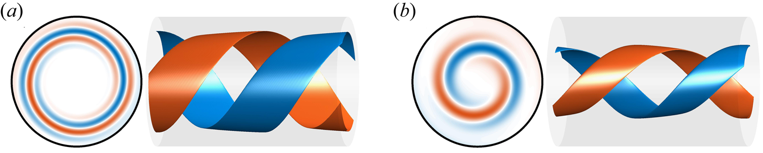
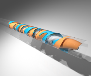
Figure 2. Colour map and isosurfaces of positive (blue) and negative (vermillion) axial vorticity  $\omega _{z}$ of the optimal helical perturbation of a pulsatile flow driven with a sine wave pulsation at $ {Re}=2000$, $A=1$ and $ {Wo}=11$. In (a) at $t_{0}/T=0.5$ and in (b) at $t/T=1$. In both panels we show a cross-section of the pipe at $z=0$ to the left; and a section $z=1.5D$ long of the pipe in the right with an isosurface of the $\pm 0.9 \max (\omega _{z} )$ at that instant of time.

Figure 3. Energy growth (solid lines) of the optimal helical perturbation according to our TGA for three different waveforms (dashed lines) for  $ {Re} =2000$ and $ {Wo}=11$. Colours and symbols correspond to three of the five waveforms defined in figure 1.
Table 1. Parametric space considered for our linear stability analysis (LSA) and transient growth analysis (TGA): range of Reynolds (Re) and Womersley (Wo) numbers and the three parameters ( $t_{m}$, $t_{ac}$, $t_{dc}$) defining our generic waveform, the total number of each parameter values ( $N_{\dotsm }$) and the total number of cases ( $N$).
$N$).

3.1. Mechanism of the perturbation growth
We first performed an LSA for a single harmonic sine wave pulsation at  $ {Re}=2000$, $ {Wo}=11$ and $A=1$ and observed that the velocity profile is instantaneously unstable for more than 50 % of the period. This can be seen in figure 4, where we show the maximum real part out of all the instantaneous eigenvalues ( $\lambda _{max}$, see (2.5)) for this case. For most of the acceleration phase, $\lambda _{max}$ is constant and negative. This corresponds to the maximum eigenvalue of Hagen–Poiseuille flow at $ {Re}=2000$ (Meseguer & Trefethen Reference Meseguer and Trefethen2003). However, for the second half of the deceleration phase and the first half of the acceleration phase, $\lambda _{max}$ is positive. The crossover occurs at ${t}/{T}\approx {0.45}$, which is very close to the optimal time to trigger the helical perturbation ( ${t_0}/{T}\approx {0.5}$) found by Xu et al. (Reference Xu, Song and Avila2021) based on a TGA for the same values of Re, Wo and $A$. These results suggest that the helical perturbation actually takes advantage of the instantaneous linear instability of the laminar velocity profile.

Figure 4. Laminar profile and instantaneous maximum eigenvalue  $\lambda _{max}$ according to our LSA for a sine wave pulsation. In yellow the instantaneous laminar profiles $U(r,t)$ at $ {Re}=2000$, $ {Wo}=11$ and $A=1$. To not interfere with one another the profiles are scaled using a scalar with arbitrary units so the all time maximum is smaller than $t/T={0.15}$, because only the development of $U(r,t)$ in time is of interest. Circles denote the radial position ( $r_{i}$) of inflection points in the velocity profile. Filled points correspond to inflection points that also satisfy the Fjørtoft criterion locally $({\partial ^2 U}/{\partial r^2})(U(r,t)-U(r_{i} ) )<0$. In red, the maximum real component out of all the instantaneous eigenvalues of the laminar profile is shown.
According to Miau et al. (Reference Miau, Wang, Jian and Hsu2017) and Nebauer (Reference Nebauer2019), the instantaneous linear instability of the SW velocity profile is related to the existence and characteristics (number or position ( $r_{i}$)) of inflection points ( ${\partial ^2 U}/{\partial r^2}=0$). An inflection point is regarded as inviscidly unstable, when the Fjørtoft criterion
 \begin{equation} \frac{\partial^2 U}{\partial r^2}\left(U-U\!\left(r_{i}\right)\right)<0 \end{equation}
is satisfied locally (Schmid et al. Reference Schmid, Henningson and Jankowski2002). Nebauer (Reference Nebauer2019) already discussed that perturbations can sit on top of these inflection points and feed energy from them. In the following, we show how the helical perturbations take advantage of this mechanism to grow. To this end, we integrated the linearised equations (2.2) forward in time using the optimal helical perturbation according to our TGA as the initial condition. We computed the production ( $P^\prime$) and dissipation ( $D^\prime$) of the kinetic energy ( $E$) contained in the perturbations as
 \begin{equation} P^{\prime} ={-}u_{r}^{\prime} u_{z}^{\prime}\frac{\partial U}{\partial r} \quad\text{and}\quad D^{\prime}={-}\frac{1}{{Re}}\boldsymbol{\nabla}\boldsymbol{u}^{\prime}:\boldsymbol{\nabla}\boldsymbol{u}^{\prime} \quad\text{where}\ \frac{\mathrm{d}E }{\mathrm{d} t} =P^{\prime} + D^{\prime} . \end{equation}
Note that  $u_{r}^{\prime }$ and $u_{z}^{\prime }$ of the helical perturbation have an axial wavenumber of $k$, and the product between the two results in structures with axial wavenumber $2k$.
$2k$.
In figure 5 (and the Supplementary Movie available at https://doi.org/10.1017/jfm.2022.681) we show colour maps of  $P^{\prime }$ and $D^{\prime }$ (only in Movie 1) structures in a $r$–
$r$– $z$-plane, and on top, the instantaneous laminar velocity profile. Strong events of production and dissipation clearly follow the radial position of inflection points in the SW profile as time marches. At each time step, the strongest production events are always bigger than the strongest dissipation events (see the Supplementary Movie). This difference between the magnitude of production and dissipation structures explains the large growth of helical perturbations. Moreover, the fact that strong production events follow the inflection points, further suggests that the helical perturbations extract their growth from them.

Figure 5. Link between inflection points in the SW profile ( $U$) and production ( $P^{\prime }$, see (3.2)) of kinetic energy contained in the helical perturbations in the $r$–
$r$– $z$-plane at $\theta =0$. Results correspond to an integration of (2.2) using the optimal helical perturbation as initial condition for a sine wave pulsation at $ {Re}=2000$, $ {Wo}=11$ and $A=1$. Yellow lines represent $U\!(r,t)$ scaled in arbitrary units and circles represent existence and location ( $r_{i}$) of inflection points. Yellow circles additionally satisfy the Fjørtoft criterion locally. We show two different instants of time: (a) mid deceleration phase at ${t_{0}}/{T}={0.5}$; (b) mid acceleration phase at ${t}/{T}={1}$. In both the production $P^{\prime }$ is normalised by the maximum value at ${t_{0}}/{T}={0.5}$, where the simulation was started.
3.2. Simple model for perturbation growth
Pulsatile pipe flow has at least two important time scales when it comes to the evolution of perturbations. One is the advective time scale ( ${D}/{u_s}$) and the other one is the pulsation period ( $T={{\rm \pi} {Re}}/{2 {Wo}^2}$ in advective time units). As Cowley (Reference Cowley1987) mentioned, for sufficiently long periods (in terms of ${D}/{u_s}$), the perturbations would see a quasi-steady velocity profile. In that case, the perturbations would have enough time to grow on top of the instantaneous linear instability before the velocity profile changes a lot and becomes stable again.
In view of these findings, we propose that the energy growth ( $G_{TGA}$) observed by Xu et al. (Reference Xu, Song and Avila2021), depends on how much and how long the SW velocity profile is linearly unstable. The instability of the velocity profile in turn depends on the existence of inflection points that satisfy the Fjørtoft criterion (Schmid et al. Reference Schmid, Henningson and Jankowski2002; Nebauer Reference Nebauer2019; Kern et al. Reference Kern, Beneitez, Hanifi and Henningson2021), as already discussed previously. With these ideas in mind we propose that from an LSA perspective the energy growth rate should scale like
 \begin{equation} \frac{E_{max}}{E_{0}}\propto G_{LSA}=e^{2\,\lambda_{i}\,T}, \end{equation}
where  $\lambda _{i}$ is the time integral
 \begin{equation} \lambda_{i}=\frac{1}{T}\int_{t_{0}}^{t_{0}+\Delta t_{u}}\lambda_{max}\left(t\right)\,\mathrm{d}t, \end{equation}
for the time window  $\Delta t_{u}$ where $\lambda _{max}>0$. The new parameter $\lambda _{i}$ is taken as a combined proxy for how much and how long the laminar profile $U$ is linearly unstable during one pulsation period.
In the following section, we compare the energy growth from our TGA with the hypothesis we propose in (3.3). We show that both calculations yield similar results, which indicates that the energy growth reported by Xu et al. (Reference Xu, Song and Avila2021) is not due to non-modal mechanisms, but to the instantaneous linear instability in the laminar profile.
4. Parametric study of perturbation growth (linear analysis)
In general, the proposed eigenvalue proxy in (3.4) depends on all the control parameters. First we explore its dependency with respect to the parameters that define the waveform ( $t_{m}$, $t_{ac}$ and $t_{dc}$), while fixing $ {Re}=2000$ and $ {Wo}=11$. Afterwards we vary the flow parameters Re and Wo. Motivated by these findings we extensively explore the parametric space and develop a simplified formulation from the generated database to approximate the energy growth of a waveform by only knowing its control parameters. We finally test this formulation with a realistic physiological waveform.
4.1. Dependency with respect to the waveform
We first focus on  $t_{m}$, which controls the asymmetry of the waveform. The smaller $t_{m}$ is, the shorter the high-velocity phase (in terms of $T$) and the larger $ {Re}_{max}$ become. From figure 6(a) it is clear that $\lambda _{i}$ increases monotonically as $t_{m}$ decreases; i.e. the waveform goes from a long high-velocity phase to a long low-velocity phase. This is because a longer low-velocity phase (smaller $t_m$) results in a longer fraction of the period $\Delta t_u$ where the profile is instantaneously unstable (figure 6b). Thus, the shorter $t_{m}$ is, the more unstable the laminar profile becomes. This conclusion is in good agreement with experimental findings of Brindise & Vlachos (Reference Brindise and Vlachos2018), who showed that flows with longer deceleration and longer low-velocity phases are more prone to transition by looking at turbulent kinetic energy and its production.

Figure 6. (a) Relationship between eigenvalue proxy  $\lambda _{i}$ (see (3.4)) and $t_{m}$. Cases correspond to $ {Re}=2000$, $ {Wo}=11$ and different lines indicate different $t_{ac}$ and $t_{dc}$. The lines correspond to the legend in panel (b). (b) Plot of $\Delta t_{u}$ or fraction of the period during which the laminar profile is instantaneously unstable for different $t_{m}$, $t_{ac}$ and $t_{dc}$. (c) Plot of $\Delta t_{u}$ for different waveforms with respect to Wo. The thin grey line corresponds to the lifetime of inflection points that satisfy the Fjørtoft criterion $\Delta t_{i}$ of WF2. (d) In colour $\Delta t_{i}$, and inflection point position span $\Delta r_{i}$ as an area, with respect to Wo for WF2.
In figure 6(a), we also show how  $\lambda _{i}$ depends on the other two waveform parameters. Recall that $t_{ac}$ and $t_{dc}$ control the slope of the acceleration and the deceleration, but do not affect $ {Re}_{max}$. It is evident from figure 6(a), that $\lambda _{i}$ is inversely proportional to both parameters, implying that steeper acceleration and steeper deceleration both lead to more unstable flows. However, the sensitivity of $\lambda _{i}$ with respect to $t_{dc}$ is larger than the sensitivity with respect to $t_{ac}$. While increasing $t_{ac}$ by a factor of four decreases $\lambda _{i}$ by only 9 %, doing the same for $t_{dc}$ decreases $\lambda _{i}$ by 16 %.
4.2. Dependency with respect to Reynolds and Womersley numbers
Our hypothesis is that  $G_{LSA}$ is proportional to the product of the period ( $T$) and the proposed eigenvalue proxy ( $\lambda _{i}$, (3.4)). Here we explore the dependency of $\lambda _{i}$ on Re and Wo and we compare $G_{LSA}$ with $G_{TGA}$ obtained by our TGA.
For both waveforms we have considered here,  $\lambda _{i}$ grows with the Reynolds number (figure 7a). In the inviscid regime ( $ {Re}\rightarrow \infty$), $\lambda _{i}$ approaches a given asymptotic value, which depends on the waveform.

Figure 7. (a) Eigenvalue proxy  $\lambda _{i}$ with respect to Re at $ {Wo}=11$ and two different waveforms (blue/green lines). (b) Eigenvalue proxy $\lambda _{i}$, (3.4), with respect to Wo at $ {Re}=2000$. (c) Energy growth $G_{LSA}$, see (3.3), with respect to Re at $ {Wo}=11$. (c) Energy growth $G_{LSA}$ with respect to Wo at $ {Re}=2000$. Orange lines correspond to the optimal transient growth $G_{TGA}$. Blue and vermillion lines correspond to waveform 1 with $t_{m}=0.45$ and $t_{ac}=t_{dc}=0.05$, whereas green lines correspond to waveform 2 with $t_{m}=0.55$ and $t_{ac}=t_{dc}=0.2$.
The dependence of  $\lambda _{i}$ on the Womersley number is more complex. From $ {Wo}\gtrsim {2}$ onwards, $\lambda _{i}>0$ (figure 7b), but the exact value at which the flow becomes unstable, depends on both the Reynolds number and the waveform. Thereafter $\lambda _{i}$ increases with Wo, until it reaches a maximum around $ {Wo}\approx {11}$. The exact $ {Wo}$ and magnitude of this maximum depend on the waveform. If Wo is now further increased, $\lambda _{i}$ decreases again but remains positive for all parameters considered here.
The dependence of  $\lambda _{i}$ on Wo is determined by the relationship between $\Delta t_{u}$ and Wo, as observed when comparing the curves in figures 7(b) and 6(c). It is the fraction of the period where the flow is unstable, $\Delta t_{u}$, what dictates the value of $\lambda _{i}$ with respect to Wo. In turn, as shown in figure 6(c), $\Delta t_{u}$ follows the trend of $\Delta t_{i}$. Here, $\Delta t_{i}$ is the fraction of the period, where the profile has only one inflection point, that additionally satisfies the Fjørtoft criterion. Thus, the presence of inflection points sets the fraction of the period where the laminar profile is unstable, which ultimately sets the level of instability $\lambda _{i}$.
For  $ {Wo}\gtrsim {3}$ the velocity profiles exhibit inflection points for more than one-quarter ( $\Delta t_{i} \gtrsim {T}/{4}$) of the pulsation period (figure 6c,d). With increasing Womersley number ( ${3}\lesssim {Wo}\lesssim 17$), the lifespan of the inflection points ( $\Delta t_{i}$) increases. The inflection points appear close to the pipe wall at the early stages of deceleration (figure 4). During the rest of the deceleration and the subsequent low-velocity phase, the inflection points move towards the pipe centreline. However, before they are able to reach the centreline, they disappear during the acceleration phase. Their movement is restricted to a radial span $\Delta r_{i} = \max (r_{i})-\min (r_{i})$ that decreases with increasing Womersley number (figure 6d). For large Wo, the evolution of the velocity profile prevents the inflection points from approaching the centreline before they die. Already from $ {Wo}\approx 11$ onwards, they remain in the vicinity of the pipe wall ( $\min (r_{i})< {D}/{4}$) and so do the perturbations that may grow on top of them. This in turn does not allow perturbations to access the more energetic flow in the central region of the pipe, resulting in a decreasing, but still bigger than zero, $\lambda _{i}$ for $ {Wo}>11$ (figure 7a). Note that at $ {Wo}>11$ perturbations can still extract energy from the inflection points but less efficiently than at $ {Wo} \approx 11$.
In order to characterise the dependency of  $G_{LSA}$, (3.3), with respect to Re and Wo we combine our knowledge of $\lambda _{i}$ with the effect of the pulsation period $T={{\rm \pi} {Re}}/{2 {Wo}^{2}}$. We observe that for intermediate Womersley numbers, $G_{LSA}$ grows monotonically with Re (figure 7c). At sufficiently high Reynolds numbers, $\lambda _{i}$ is more or less constant (figure 7a) and $G_{LSA}$ ends up following the exponential relationship between $T$ and Re.
The combined effects of  $\lambda _{i}$ and pulsation period set the point of maximum growth at $ {Wo}\approx 7.5$ (figure 7d). Depending on the waveform or the Reynolds number, the exact position of this maximum with respect to Wo can vary slightly. Interestingly the region close to $ {Wo}\approx 7.5$ matches the point of maximum transient growth for a flow driven with a sine wave pulsation (Xu et al. Reference Xu, Song and Avila2021), and it is close to the point of maximum growth of perturbations in pulsatile channel flow (Pier & Schmid Reference Pier and Schmid2017). It is at this particular Wo, where the competing effects of shorter pulsation periods (in terms of advective time units) and higher level of average instability of the laminar profile make the flow more susceptible for perturbations to grow.
In figures 7(c) and 7(d) we show that  $G_{LSA}$, (3.3), approximates the optimal transient growth $G_{TGA}$, (2.6), reasonably well at several Re and Wo. Note that we do not use any constant to match the two lines, but directly show $G_{LSA}$ as computed according to (3.3). This shows that the energy growth of the helical perturbation is related to the instantaneous instability of the laminar profile and confirms our hypothesis. It is the instantaneous instability of the laminar profile what yields the outstanding perturbation growth observed in the TGA of Xu et al. (Reference Xu, Song and Avila2021), as long as $T$ is sufficiently long (in terms of advective time units). In our results, $G_{TGA}>G_{LSA}$, as expected. This means that, on top of the modal growth that comes from the instantaneous instability, the perturbation can further grow due to additional non-modal mechanisms.
4.3. Gradient descent
In this section, we exploit the knowledge gained on perturbation growth so far, to develop a simple parametric model. Specifically we model the dependency of the perturbation growth on the governing parameters by approximating (fitting) our two sets of LSA and TGA computations listed in table 1 with the expression
 $$\begin{gather} \log G_{g} = s \sigma {Re} + bi_{3}, \end{gather}$$
 $$\begin{gather}s = bi_{2} + w_{m} t_{m} + w_{ac} t_{ac} + w_{dc} t_{dc}, \end{gather}$$
 $$\begin{gather}\sigma = [w_{1} \left( {Wo}-b_{1}\right) + w_{2}\left( {Wo} -bi_{1}\right)^{2}] \exp{\left({-}w_{3}{Wo}\right)}. \end{gather}$$
The parameter  $G_{g}$ is our approximation to $G_{LSA}$ or $G_{TGA}$. We use an exponential dependence on Re, an assumption motivated by (3.3), where we suggest that the perturbation growth scales exponentially with the product of the pulsation period $T$ and $\lambda _{i}$. As we show in figure 7(a), at a sufficiently high $ {Re}$, $\lambda _{i}$ reaches a constant value and $G_{LSA}$ (and, therefore, $G_{g}$) follows the exponential relationship with $ {Re}$ that comes from $T={{\rm \pi} {Re}}/{2 {Wo}^2}$ (figure 7b). Further, we assume that the slope of this relationship is given by the product of (4.2) and (4.3). The function $\sigma$ approximates the shape of $G_{LSA}$ with respect to Wo that is shown in figure 7(d). We now know that at $ {Wo}\approx 11$, $\lambda _{i}$ peaks, whereas $T$ always decreases as $ {Wo}$ increases. From these two ideas, we select a function $\sigma$ that goes to zero as $ {Wo}\rightarrow 0$ and $ {Wo} \rightarrow \infty$. The function $s$ accounts for the dependency of $G_{g}$ on the shape of the pulsation waveform (i.e. $t_{m}$, $t_{ac}$ and $t_{dc}$). From figures 6(a) and 6(b), $\lambda _{i}$ appears to depend linearly on each of the three parameters (at least for the values we consider here) and, henceforth, $G_{LSA}$ depends exponentially on each of them. Although the results in previous sections suggest cross-dependencies between the parameters, we ignore these in our model equation for the sake of simplicity.
We approximate  $G_{g}$ by looking for the set of weights ( $w_{i}$) and biases ( $bi_{i}$) in (4.1)–(4.3) that minimise the error
 \begin{equation} \epsilon=\frac{1}{N} \sum^{N}_{n=1} \left(\log G-\log G_{g}\right)_{n}^2, \end{equation}
where  $N$ is the total number of data items to fit (table 2). We produce two fits, one to the LSA results where $G=G_{LSA}$ and another to the TGA results where $G=G_{TGA}$. We initialise each fit with the vector $\pmb {x}^{0}$ that is filled with random guesses of weights and biases with values between zero and one. Then we use a gradient descent method to find the vector $\pmb {x}^{i}$ that minimises (4.4). Iterations are performed until a minimum is reached. At iteration $i$ the weights and biases are updated as
 \begin{equation} \pmb{x}^{i+1}=\pmb{x}^{i} - \eta \sum^{N}_{n=1} \frac{\mathrm{d}\epsilon^{n}}{\mathrm{d}\kern0.7pt \pmb{x}^{i}} , \end{equation}
where  $\eta$ is a learning parameter that is dynamically adjusted so that the error $\epsilon (\pmb {x}^{i+1})<\epsilon (\pmb {x}^{i})$. We consider the case as converged when the error decreases to less than $10^{-10}$ for consecutive iterations.


The quality of the fit is visualised in figure 8. The horizontal axis represents the number of the case, where the list of cases is ordered in the sense of increasing first Re, then Wo and finally  $t_{m}$, $t_{ac}$ and $t_{dc}$ as in table 1. This explains why the data appear in packets of functions that look similar to the shape of the function shown in figure 7(c).

Figure 8. Results of our fit using the gradient descent method. (a) Fit of  $G_{LSA}$ (see (3.3))–(4.1). Hollow circles are individual results of the LSA for all the parameters considered (first row in table 1). Black dots are the fit of the method. In each horizontal location we plot just one case with a given combination of Re, Wo, $t_{m}$, $t_{ac}$ and $t_{dc}$. The cases are ordered in increasing sense of first Re then Wo and finally $t_{m}$, $t_{ac}$ and $t_{dc}$. (b) Same fit but for $G_{TGA}$ (second row in table 1).
Note that the fit performs poorer as Re increases. We know that Re also has an effect on  $\lambda _{i}$, as shown in figure 7(b). However, the formulation we have proposed ignores this, and other cross-dependencies, as it only considers the dependency of $G$ on Re coming from $T$. Despite these differences, the error is of the order of $10^{-4}$ for both fits.
The final weights of the two fits (table 2) show that  $t_{m}$ has a greater effect on the energy growth compared with $t_{ac}$ and $t_{dc}$, because $|w_{m}|>|w_{dc}|>|w_{ac}|$. The smaller $t_{m}$, $t_{ac}$ and $t_{dc}$ are, the bigger the energy growth is, because $w_{m}< w_{ac}< w_{ac}<0$. Note that the two fits do not reach the same values for all weights and biases. This is due to the differences between the two sets of data, and the choices we use for the fitting formula. The weights are the key parameters, as they quantify the importance of some parameters with respect to others, and are found to be very similar for the fits to $G_{LSA}$ and $G_{TGA}$.
The fits allow us to generalise the dependency of  $G_{LSA}$ and $G_{TGA}$ on all the control parameters for all the waveforms we have considered here. With this tool one can infer how much a helical perturbation can grow in a given pulsatile pipe flow by only knowing the waveform of the pulsation and the control parameters Re and Wo.
4.4. Physiological waveform
As a test to our observations, we study the behaviour of a laminar profile driven by a physiological waveform. To that end a particular signal presented in the physiological study of Bürk et al. (Reference Bürk, Blanke, Stankovic, Barker, Russe, Geiger, Frydrychowicz, Langer and Markl2012) was selected (figure 9a). In their study, they measured the mean velocity of blood flow at different sections of the aorta in several patients. In our study the signal for the descending aorta section of a young volunteer was fitted using  $N_{F}=8$ Fourier modes. The resultant Fourier mode coefficients for the physiological waveform (1.1) are presented in table 3. We compute the waveform parameters by measuring the time span between the half point of the acceleration and deceleration ( $t_{m}\approx 0.279$). In addition, we measure half the length of the acceleration ( $t_{ac}\approx 0.108$) and the deceleration ( $t_{dc}\approx 0.141$). By introducing these parameters to expression (4.1) and using the weights listed in table 2, we generated a guess of the energy growth on top of the laminar velocity profile in the physiological waveform (figure 9b,c). In addition, we performed LSA (solid blue line) and TGA (red dots) to probe the accuracy of the fits.

Figure 9. Results and fit of the energy growth of helical perturbations on a laminar profile driven with a physiological waveform. (a) Physiological waveform defined by coefficients of table 3 in blue, compared with a sine wave pulsation in yellow. (b) Evolution of energy growth  $G$ with Re at $ {Wo}=12$ for the physiological waveform. The blue solid line corresponds to $G_{LSA}$ and the blue dotted line is a guess using the expression (4.1) with the weights in the first row of table 2. Filled vermillion points correspond to TGA results and the dotted vermillion line corresponds to a guess using the expression (4.1) with the weights in the second row of table 2. (c) Evolution of energy growth $G$ with respect to Wo at $ {Re}=2000$ for the physiological waveform. Lines and symbols correspond to the same cases as in (b).
Table 3. Fourier coefficients ( $a_i$, $b_i$) used to approximate the physiological waveform of Bürk et al. (Reference Bürk, Blanke, Stankovic, Barker, Russe, Geiger, Frydrychowicz, Langer and Markl2012).
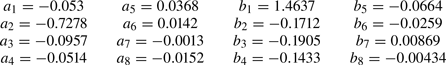
The fitting of expression (4.1) gives a good estimate of the growth of perturbations for the physiological waveform, even though all data used to obtain the fit coefficients are for  $t_{m}\geq 0.3$ (table 1). Larger errors are found for $ {Wo}\leq 10$ and correspond to our definition of $\sigma$ in (4.3). Future analyses may improve this equation to better capture the behaviour at low Womersley numbers.
Figures 9(b) and 9(c) confirm some of the ideas proposed in this paper. First, the energy growth of the helical perturbations is related with the instantaneous instability of the laminar profile due to the presence of inflection points. This is confirmed by the similarity of  $G_{TGA}$ with $G_{LSA}$. Second, the shape of the pulsation waveform has an important effect on the energy growth. This is shown in figure 6(a) and evident from the non-negligible values of $w_{m}$, $w_{ac}$ and $w_{dc}$ in our fits.
5. DNS
In order to assess the relevance of our findings from the linear analyses to turbulence transition, we performed 80 DNS of pulsatile pipe flow. As detailed in table 4, we considered 8 different waveforms and 10 different initial conditions, while keeping  $ {Re}= 2000$ and $ {Wo}= 11$ fixed.
Table 4. Parametric space considered in our nonlinear study at fixed  $ {Re}=2000$ and $ {Wo}=11$. The different waveforms (WF) are defined by the parameters $t_{m}$, $t_{ac}$ and $t_{dc}$. For each waveform, 10 simulations were performed using different initial conditions. The number of DNS runs that remained turbulent after 20 pulsation periods is given by $N_{surv}$.
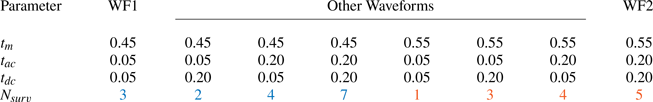
The decision for these specific parameters is two-fold. First,  $ {Wo}\approx 11$ is a value typically found in our main target application, the flow in the bigger vessels of the human cardiovascular system (Les et al. Reference Les, Shadden, Figueroa, Park, Tedesco, Herfkens, Dalman and Taylor2010). Second, $ {Wo}=11$ offers a good compromise between turbulence transition and turbulence survival. At lower $ {Wo}\lesssim 8$, perturbations exhibit higher transient growth, but once triggered, turbulence quickly decays during the first acceleration (Xu et al. Reference Xu, Warnecke, Song, Ma and Hof2017; Xu & Avila Reference Xu and Avila2018; Feldmann et al. Reference Feldmann, Morón and Avila2021). At higher $ {Wo}\gtrsim 15$, the dynamics of turbulence are similar to those observed in steady pipe flow and the waveform is not expected to have much influence on them.
The computational domain is  $L_z=50 D$ long and, following Feldmann et al. (Reference Feldmann, Morón and Avila2021), the simulations are initialised at $t_{0}$ with the corresponding SW velocity profile disturbed with the optimal helical perturbation obtained from our TGA. In numerical simulations with global initial perturbations (not shown here), the perturbations grow and trigger turbulence in the whole domain. This turbulence then localises into patches that tend to interact and decay. Here we localise the initial perturbation in our DNS to $5D$ in $z$ direction, because we aim at studying the turbulence survival of isolated puffs. The shape of the perturbation is given by the TGA and is different for each pulsation waveform. For each waveform, we perform different DNS by changing the magnitude of the initial perturbation in 10 steps from $5\times 10^{-3}$– $5\times 10^{-2}$ in terms of $u_s$. We observed that at lower magnitudes (e.g. $\lesssim 5\times 10^{-4}$), some cases do not transition to turbulence (not shown here). For turbulence to appear, the product $G_{LSA}$ times the initial amplitude of the perturbation must be of the order of ${O}(1)$ or higher.
In order to detect, track and quantify the presence of localised turbulence in the pipe, we define the turbulence intensity as
 \begin{equation} \varOmega\left(z,t\right) = \langle\omega_{z}^{2}\rangle_{r,\theta} = \frac{1}{{\rm \pi} R^{2}}\int_{0}^{R}\int_{0}^{2{\rm \pi}}\omega_{z}^{2}\, r\, \mathrm{d}r\, \mathrm{d}\theta \end{equation}
based on the axial vorticity component ( $\omega _z$). For $\varOmega > 0.05 ({u_{s}^2}/{D})$, we consider the flow as locally turbulent and otherwise as laminar. This allows us to define a turbulent fraction for the entire pipe domain
 \begin{equation} F_{turb}\left(t\right) = \frac{L_{turb}\left(t\right)}{L_{z}} , \end{equation}
where  $L_{turb}$ represents the integral length of the pipe for which the condition $\varOmega > 0.05$ is satisfied.
Figure 10 shows the temporal evolution of  $F_{turb}$ for all 80 DNS we have performed. It is clear that all the different initial conditions were able to trigger a turbulent state that survives for at least one pulsation period. During the first deceleration phase, the turbulent fraction grows quickly to almost 50 % in all cases.

Figure 10. Turbulent fraction  $F_{turb}$, (5.2) in all our DNS with respect to time: (a) $t_{ac} = 0.05,\ t_{dc} = 0.05$; (b) $t_{ac} = 0.05,\ t_{dc} = 0.20$; (c) $t_{ac} = 0.20,\ t_{dc} = 0.05$; (d) $t_{ac} = 0.20, t_{dc} = 0.20$. It corresponds to the fraction of the pipe with $\varOmega >0.05$, see (5.1). Here $F_{turb}=1$ means a fully turbulent pipe, whereas $F_{turb}=0$ denotes a fully laminar pipe. Results correspond to $80$ DNS: for 8 different waveforms, or different $t_{ac}$, $t_{dc}$ and $t_{m}$; and $10$ different initial conditions. In panels find the cases with the same pair of $t_{ac}$, $t_{dc}$. The colours and symbols of the lines denote different $t_{m}$. In each panel, and for each $t_{m}$ we show in a thick line the instantaneous mean turbulent fraction of the cases (out of the initial 10) that have not yet relaminarised. The thickness of the mean turbulent fraction decreases whenever 1 of the 10 cases relaminarises. In thin lines see the evolution for the cases that relaminarise at $t<20 T$. With numbers we denote the number of cases where turbulence is sustained for $t\leq 20 T$.
Cases with smaller  $t_{m}$ exhibit faster growing $F_{turb}$ in the initial transient when compared with cases with larger $t_{m}$. Once the perturbation has triggered turbulence ( $t\gtrsim 1.5T$), the turbulent fraction remains at roughly 30 %, but is clearly modulated by the pulsation in all cases (figure 10). However, cases with smaller $t_{m}$ reach a slightly higher turbulent fraction, whereas cases with larger $t_{m}$ are slightly less turbulent. Both observations are in good agreement with our linear analyses, which predicts larger energy growth for smaller $t_{m}$.
From experiments and DNS at  $ {Re}=2000$, we know that turbulence is expected to decay at some point in time (Xu et al. Reference Xu, Warnecke, Song, Ma and Hof2017; Xu & Avila Reference Xu and Avila2018). Thus, we stopped our simulations as soon as the flow relaminarised in the entire pipe ( $F_{turb}=0$) and remained laminar for another full period. Otherwise, we continued all DNS for 20 pulsation periods ( $520({D}/{u_s})$). The number of runs for which turbulence survived the full simulation time ( $20T$) is detailed in table 4 and figure 10. Out of the 10 different initial conditions, 1–7 runs remain turbulent depending on the waveform.
The waveform parameters also have an effect on relaminarisation, as presented in table 4 and figure 10. For large  $t_{m}$ only 13 out of 40 cases remain turbulent for the full 20 periods, whereas 16 out of 40 cases remain turbulent when $t_{m}$ is small. Regarding the other two parameters, for large $t_{dc}$ 17 out of 40 cases remain turbulent for the full 20 periods, whereas 12 out of 40 cases remain turbulent when $t_{dc}$ is small. For large $t_{ac}$ 20 out of 40 cases remain turbulent for the full 20 periods, whereas 9 out of 40 cases remain turbulent when $t_{ac}$ is small. According to our linear analysis, pulsations with small $t_{m}$, $t_{ac}$ and $t_{dc}$ show higher perturbation growth. However, according to our DNS, they are more likely to cause relaminarisation once the flow is turbulent. In contrast, pulsations with larger $t_{m}$, $t_{ac}$ and $t_{dc}$ are less likely to transition to turbulence, but more prone to remain turbulent once turbulence is triggered.
As a typical example for the dynamics of the localised turbulent regions in our DNS, we show a space–time representation of  $\varOmega$ for two selected cases in figure 11. The red structures indicate high values of $\varOmega$ and represent localised turbulent puffs. The puffs are clearly modulated by the pulsation. During the deceleration phase the puffs usually increase in length and magnitude. The puffs further elongate and even split during the rest of the deceleration and low-velocity phases. The acceleration phase, on the other hand, has a stabilising effect. The turbulent puff decreases in strength and elongates downstream, resulting in the white tendrils shown figure 11. Right after the acceleration phase, $\varOmega$ has decreased by roughly one order of magnitude and the remaining structures are much shorter. This is the critical moment in terms of relaminarisation. If the remaining $\varOmega$ is too small, the additional energy production during the following deceleration phase is not sufficient to trigger a new turbulent puff. The definite decay can happen here (i.e. in the deceleration) or later in the next period. In the second case, the remaining structures can still grow during the following deceleration (figures 11a and 10), but they do not attain a sufficient magnitude to further survive and, thus, ultimately decay.

Figure 11. Space–time diagram of the cross-section integral of axial vorticity square (5.1): (a) a flow driven with  $t_{ac}=t_{dc}=0.05$ and $t_{m}=0.45$ (WF1); (b) a flow driven with $t_{ac}=t_{dc}=0.2$ and $t_{m}=0.55$ (WF2). The results correspond to a DNS in a $50D$ pipe at $ {Re}=2000$ and $ {Wo}=11$. The simulations are initialised with the optimum perturbation scaled to $|\boldsymbol {u}^\prime _{0}|\approx 3\times 10^{-2}$ of magnitude and localised in a span of $5D$. The figure is presented with respect to a moving frame, moving with the pulsation velocity $u_{b}$.
6. Conclusions
In this paper we have shown how the helical perturbations reported by Xu et al. (Reference Xu, Song and Avila2021) are linked to the instantaneous linear instability of the laminar velocity profile in pulsatile pipe flow. This instability emerges from the presence of inflection points in the laminar profile and their characteristics, as suggested by Nebauer (Reference Nebauer2019). We have shown that two requirements must be fulfilled for the helical perturbations to grow. The first is the existence of inflection points that satisfy the Fjørtoft criterion and render the laminar profile instantaneously unstable for a sufficiently long fraction of the period. This is the case for  $ {Wo}\gtrsim 3$ and $A\gtrsim 0.5$. The second is that the laminar profile evolves much slower than the perturbations, which is the case for $ {Wo}\lesssim 17$. In the range of $ {Re}$ investigated, if these two requirements are met, the laminar profile is highly susceptible to the growth of perturbations during that fraction of the period when it presents inflection points. This usually happens during the deceleration and low-velocity phases, where the helical perturbations lock their radial position with the inflection points, resulting in outstanding energy growth as they move towards the centreline of the pipe.
Our results show that the large transient growth of perturbations observed by Xu et al. (Reference Xu, Song and Avila2021) and Kern et al. (Reference Kern, Beneitez, Hanifi and Henningson2021) is due to the instantaneous linear instability of the laminar profile. The link between LSA and TGA, suggests that, for similar unsteady shear flows, at these  $ {Re}$ and $ {Wo}$, no transient growth or optimal time-dependent modes analyses are needed in order to infer the growth of perturbations.
The waveform of the pulsation can change the lifetime, the radial span and the characteristics of these inflection points. For waveforms with longer low-velocity phases (smaller  $t_{m}$), the inflection points remain a longer fraction of the period in the flow and give more time for the perturbations to grow. In addition, the more abrupt the deceleration and acceleration phases are (smaller $t_{dc}$ and smaller $t_{ac}$), the higher the chances are for perturbations to grow. This means that, by just knowing the waveform and the flow parameters (Re and Wo), one can easily estimate the growth of perturbations for a given pulsatile pipe flow without even computing the laminar velocity profile. We demonstrated this by fitting the results of our stability analyses for 14 000 different set-ups to a simple formula. This formula is motivated by physical interpretations and observations from our numerical results, where cross-dependencies between the parameters and other features are ignored. We used this formula to predict the expected energy growth for a physiological waveform with good agreement.
By performing several DNS of pulsatile pipe flow, we showed that helical perturbations can quickly trigger turbulence, for all the waveforms considered here. In accordance with the energy growth predicted by the LSA and TGA, this transition happens faster or slower depending on  $t_{ac}$, $t_{dc}$ and $t_{m}$. Cases with longer low-velocity phases and steeper acceleration/deceleration show higher peaks of turbulent fraction than cases with longer high-velocity phases.
We also reveal the effect the waveform has on turbulence survival once turbulence is triggered. Different to what its effect on perturbation growth suggests, flows driven with waveforms with small values of  $t_{dc}$, $t_{ac}$ and $t_{m}$ actually promote turbulence decay. This suggests that, in the nonlinear regime, the waveform has additional effects. For example, waveforms which are more susceptible to perturbation growth are also more prone to cause relaminarisation. It is our goal to further study these effects by performing additional DNS of pulsatile pipe flows with different Re, Wo and waveforms. Flows in cardiovascular vessels are affected by wall compliance and the complex geometry of the cardiovascular system, to name a few. It is also our goal to extend this analysis and investigate if geometry and compliance affect the behaviour of inflection points or introduce further instabilities in the flow.
Supplementary movies
Supplementary material and movies are available at https://doi.org/10.1017/jfm.2022.681.
Acknowledgements
Furthermore, the authors appreciate many fruitful and inspiring discussions with the members of the research unit and the fluid modeling and simulation group at ZARM.
Funding
This work was funded by the German Research Foundation (DFG) through the research unit Instabilities, Bifurcations and Migration in Pulsating Flow (FOR 2688) under grant AV 120/6-1, which is gratefully acknowledged. Computational resources were provided by the North German Supercomputing Alliance (HLRN) through the project hbi00053, which are also gratefully acknowledged.
Declaration of interests
The authors report no conflict of interest.


 Open access